Article

Seasonal and Multi-Year Wind Speed Forecasting Using BP-PSO Neural Networks Across Coastal Regions in China

by
Shujie Jiang
1,
Jiayi Jin
1,* and
Shu Dai
2
1
School of Energy and Engineering, University of Shanghai for Science and Technology, Shanghai 200093, China
2
Shanghai Investigation, Design, and Research Institute, Shanghai 200335, China
*
Author to whom correspondence should be addressed.
Sustainability 2025, 17(22), 10127; https://doi.org/10.3390/su172210127
Submission received: 7 October 2025 / Revised: 4 November 2025 / Accepted: 5 November 2025 / Published: 12 November 2025
(This article belongs to the Section Sustainable Engineering and Science)

Abstract

Accurate short-term wind speed forecasting is essential for the sustainable operation and planning of coastal wind farms. This study develops an improved BP-PSO hybrid model that integrates particle-swarm optimization, time-ordered walk-forward validation, and uncertainty quantification through block-bootstrap confidence intervals and Monte-Carlo dropout prediction intervals. Using multi-year and seasonal datasets from four coastal stations in China—from Bohai Bay (LHT, XCS, ZFD) to Zhejiang Province (SSN)—the proposed model achieves high predictive accuracy, with RMSE values between 1.09 and 1.54 m/s, MAE between 0.79 and 1.10 m/s, and R2 exceeding 0.70 at most sites. The multi-year configuration provides the most stable and robust results, while autumn at ZFD yields the highest errors due to intensified turbulence. XCS and SSN exhibit the most consistent performance, confirming the model’s spatial adaptability across distinct climatic regions. Compared with the ARIMA and persistence baselines, BP-PSO reduces RMSE by over 50%, demonstrating improved efficiency and generalization. These results highlight the potential of intelligent data-driven forecasting frameworks to enhance renewable energy reliability and sustainability by enabling more accurate wind-power scheduling, grid stability, and coastal energy system resilience.

1. Introduction

Wind energy, as a clean and renewable source, plays an important role in mitigating global energy crises and climate change challenges. Offshore wind resources have attracted increasing attention due to their higher energy density, stronger and more stable wind speeds, and reduced land-use conflicts compared to onshore projects [1,2]. According to the Global Wind Energy Council (GWEC), the global installed wind capacity reached 906 GW by the end of 2022, with offshore wind contributing 8.8 GW of new capacity [3]. China led the world in new offshore installations, accounting for more than 70% of the global total, driven by strong policy incentives and rapid coastal infrastructure development [4,5]. These trends reflect the strategic role of offshore wind in national energy transitions, especially in the context of achieving carbon neutrality targets.
Wind speed forecasting methods can generally be classified into four categories as follows: statistical models, physical models, machine learning (ML) models, and hybrid approaches. Statistical models, such as autoregressive integrated moving average (ARIMA) and persistence models, are computationally efficient but struggle to capture the nonlinear and non-stationary nature of wind [6,7]. Physical models, including mesoscale numerical weather prediction (NWP) systems, simulate atmospheric processes using fluid dynamics but demand substantial computational resources and often lack the spatial resolution to represent local wind variations [8,9].
ML models have shown increasing promise in wind speed forecasting by learning nonlinear relationships directly from historical data without explicit physical assumptions. Popular ML approaches include support vector machines (SVM) [10], random forests (RF) [11], and backpropagation (BP) neural networks [12]. In recent years, deep learning (DL) models, such as convolutional neural networks (CNN), long short-term memory (LSTM) networks, gated recurrent units (GRU), and transformer-based architectures, have further enhanced accuracy by capturing temporal dependencies and multi-scale patterns in meteorological time series [13,14,15]. Moreover, these data-driven methods are increasingly combined with signal decomposition techniques or optimization algorithms to improve their robustness under highly variable offshore conditions [16].
Reliable wind speed forecasting is fundamental to offshore wind farm development, influencing turbine site choosing, power output estimation, and investment planning. Recent research on short-term wind field dynamics demonstrates that complex terrain flow environments require hybrid machine-learning and physics-informed approaches [17]. BP neural networks are widely used for their nonlinear modeling capacity [18], but they suffer from slow convergence and local minima entrapment [19]. Particle swarm optimization (PSO), inspired by swarm intelligence, has been employed to globally optimize BP parameters, improving convergence speed and prediction accuracy [20,21].
Hybrid forecasting approaches have emerged to combine complementary strengths of multiple algorithms. Examples include empirical mode decomposition-BP (EMD-BP) models enhanced by PSO [22], CNN-LSTM architectures for spatial–temporal feature extraction [23], and attention-based transformer networks for robust forecasting under high variability [15]. While these approaches often achieve high accuracy, they face notable limitations: most require large, high-quality datasets, which are often unavailable for offshore stations [24]; many DL models have high computational costs, limiting real-time application [25]; most studies focus on single-site predictions, with limited evaluation of cross-regional transferability [26]; and seasonal variability is often underexplored, despite its significant influence on wind regimes [27].
This study proposes a data-efficient wind speed forecasting framework based on a BP neural network optimized via PSO to address these gaps. The BP-PSO model combines the strong nonlinear fitting capacity of BP with the global search ability of PSO, enhancing convergence and avoiding local minima. Two modeling strategies are implemented: a multi-year model trained on three consecutive years of data to capture long-term temporal dependencies and seasonal models trained separately on season subsets to better account for intra-annual variability. These models are evaluated at four coastal stations in China with distinct geographic and climatic conditions to assess both seasonal adaptability and spatial generalization. The results show that while multi-year models offer more stable generalization, seasonal models respond better to short-term fluctuations, with both approaches achieving acceptable accuracy. This confirms the BP-PSO framework as a robust, interpretable, and computationally efficient tool for short-term offshore wind speed forecasting, with potential applicability to other regions facing similar data and operational constraints.

2. Materials and Methods

2.1. Previous Works

Several machine learning techniques have been widely adopted for wind speed prediction, each with distinct characteristics. Linear regression (LR) offers interpretability and simplicity but fails to capture nonlinear wind dynamics [28]. Support vector machines (SVM) are effective for small sample and nonlinear problems [10], though they are sensitive to hyperparameters and computationally intensive. Random forests (RF) are robust to noise and suitable for high-dimensional data [11]; however, they lack temporal modeling capabilities and may overfit. K-nearest neighbors (KNN) require minimal training but suffer from high computational cost during prediction and perform poorly with large datasets [29]. Long short-term memory networks (LSTM) are well-suited for time series forecasting and capturing long-term dependencies but require large training datasets, are prone to overfitting, and demand high computational resources [14].
In contrast, the BP-PSO method offers several notable advantages. By leveraging PSO to optimize the initial weights and biases of the BP neural network, the model avoids common issues such as local minima and slow convergence. The BP-PSO model exhibits strong nonlinear modeling capabilities, good generalization across seasonal and multi-year datasets, and comparatively lower computational cost than deep learning models like LSTM. These characteristics make BP-PSO a reliable and efficient solution for wind speed prediction under both stationary and fluctuating conditions.

2.2. Overall Framework

The proposed methodology consists of four sequential stages: preprocessing and normalization of hourly wind speed data; short-term forecasting using a BP neural network optimized by PSO. This approach exploits the BP model’s capacity to capture temporal patterns. Figure 1 shows the framework of proposed wind resource assessment method.
In this framework, the choice of a BP neural network as the core prediction model is motivated by its strong ability to capture nonlinear relationships in meteorological data. While models such as Support Vector Regression and Long Short-Term Memory have shown comparable performance in certain scenarios, BP networks offer superior interpretability and computational efficiency for short-term horizon predictions, particularly when enhanced by global optimizers such as PSO. The PSO algorithm adjusts the weights and biases of the BP network by minimizing the prediction error on a validation set, thus avoiding entrapment in local minimum.
The forecasting task is defined as short-term, one-hour-ahead wind speed prediction. Specifically, the model uses a 24 h historical window of wind speed observations as input to predict the wind speed one hour into the future ( W = 24 h, H = 1 h). This configuration balances short-term responsiveness and the need to capture diurnal variations. The model is univariate, it relies solely on wind speed measurements without additional exogenous predictors such as wind direction, pressure, or NWP variables. All input features are normalized to [0, 1] before training.

2.3. Backpropagation Neural Network and Particle Swarm Optimization Algorithm

BP neural networks were selected due to their simplicity, low computational demand, and effective nonlinear fitting ability for time-series data. While advanced models such as LSTM or GRU could potentially improve temporal dependency learning, their need for larger datasets and tuning complexity made BP more suitable given the limited hourly wind speed data from a single meteorological station. Moreover, the interpretability and compatibility of BP with PSO optimization offered a practical trade-off between complexity and performance.
The BP neural network consists of an input layer, one or more hidden layers, and an output layer. Its fundamental principle includes forward propagation and error backpropagation. According to Caterini [30], for the k-th training sample, the neuron output in the hidden and output layers can be described as:
H j k = f i w i j 1 x i k + b j 1
O m k = f j w j m 2 H j k + b m 2
where H j ( k ) is output of hidden neuron j , x i ( k ) is input features of sample, k ,   O m ( k ) is output of neuron m, w i j ( 1 ) , w j m ( 2 ) are weights between input-hidden and hidden-output layers, b j ( 1 ) , b m ( 2 ) are biases, f ( ) is activation function.
The weight update rule during backpropagation is:
w i j 1 w i j 1 η E w i j 1
where η is the learning rate.
The PSO algorithm is employed to optimize the parameters by minimizing the validation loss function. The convergence of PSO is evaluated using a swarm size of 30 particles and 100 iterations.
According to Foqaha [31], the PSO update rules can be described as:
x i t + 1 = ω x i t + c 1 p i t + c 2 g i t
v i t + 1 = v i t + η p i t x i t
where the inertia weight is ω , c 1 and c 2 are the cognitive and social coefficients, and η is the velocity coefficient.
The squared error for sample k is given by:
E k = 1 2 m ( O m k y m k ) 2
Total training error:
E = k E k
where y m ( k ) is the expected (true) output.
Short-term forecasting is defined by an input window W = 24 h and a forecast horizon H = 1 h. Unless otherwise stated, no exogenous variables are used (BP-PSO operates at wind speed only).
The hyperparameter settings for the BP neural network are summarized in Table 1. These values are chosen based on empirical optimization and prior sensitivity analysis. As shown in Table 1, the upper and lower limits of BP parameters are set as follows: the number of neural network layers = 2, the number of neurons in the first layer is 150, the number of neurons in the second layer is 50, the learning rate is 0.000032, the batch size is 32, and the dropout rate is 0.1–0.3. We use hourly wind speed data from 2019 to 2022. The dataset is split chronologically as follows: 2019–2021 for training and 2022 as the held-out test year. The first 75% of the training set is taken and the last 25% of the training set is taken. A two-layer MLP with a small learning rate, mini-batch size, and light dropout balances model capacity and regularization, yielding stable convergence and better generalization on noisy data.
The BP-PSO model consists of two hidden layers with ReLU activation. The number of neurons per layer ( h 1 , h 2 ), dropout ratio, learning rate, and L2 regularization coefficient are treated as tunable hyperparameters. Their optimal values are obtained through particle swarm optimization (PSO) by minimizing the validation RMSE under an expanding-window walk-forward cross-validation performed only on the training set (2019–2021). The test set (2022) is used exclusively for final evaluation.
The PSO search space is defined as h 1 64 ,   256 , h 2 32 ,   128 , dropout 0.10 ,   0.30 , l r [ 10 4 ,   3 × 10 3 ] , L 2 [ 10 6 ,   10 3 ] . The swarm size and maximum iteration are set to 30 and 100, respectively, with a fixed random seed of 42 to ensure reproducibility. Preliminary grid search was used only to determine the fixed network depth (2 hidden layers) and activation function prior to PSO tuning.
The key parameters of the Particle Swarm Optimization algorithm are listed in Table 2. As shown in Table 2, the PSO parameters are set to ω = 0.5, c1 = 1.8, c2 = 2.0. The configuration uses moderate inertia with near-classical cognitive and social coefficients to balance global exploration and local exploitation, promoting a robust and convergent search.
The ω is inertia weight, which controls global and local search tendency, c1 is cognitive coefficient, reflecting particle’s own best position influence, and c2 is social coefficient, reflecting swarm’s best global influence.
Prediction errors primarily stem from the following three sources: local meteorological anomalies such as typhoons or sudden wind shifts, which are difficult to model using deterministic ML. Additionally, PSO optimization, while generally stable, is sensitive to initial particle positions and inertia parameters, which may lead to local optima in complex search spaces.

2.4. Walk-Forward Cross-Validation

To avoid temporal leakage, hyperparameters are selected using an expanding-window walk-forward CV on the training years (2019–2021). Let the training series length be N ; we define S sequential validation windows of length 0.1 N near the end of the training period. For each split s , we train on [ 1 , t s ) and validate on [ t s , t s + V ) , without shuffling, and we minimize the average validation RMSE across all splits. The final model is then retrained on the full 2019–2021 data with the selected hyperparameters and evaluated once in 2022.

2.5. Baseline Models

To provide a fair reference for evaluating the proposed BP-PSO predictor, two classical baseline models were implemented under the same data split (Train: 2019–2021, Test: 2022) and short-term forecasting configuration.
(1)
Persistence model
The persistence model assumes that the wind speed in the next step equals the most recent observation. Despite its simplicity, persistence provides a strong benchmark for short-term wind forecasting, as it reflects the natural autocorrelation of wind series and defines a lower bound for achievable improvement.
y t + 1 = y t
(2)
ARIMA model
The autoregressive integrated moving average (ARIMA) is a widely used statistical model for univariate time series.
For this study, ARIMA models with orders ( p , d , q ) { ( 1,1 , 1 ) , ( 2,1 , 2 ) , ( 3,1 , 2 ) } were fitted on the training years (2019–2021) and used to forecast the 2022 test year. The model parameters were selected by minimizing the Akaike Information Criterion (AIC).
ARIMA provides a classical linear baseline that captures short-term temporal dependencies but lacks the nonlinear representation capability of neural networks.

2.6. Data and Site Selection

The Yangtze River Estuary near Zhejiang and the Bohai Sea off Liaoning and Yantai possess abundant offshore wind energy resources, with several commercial wind farms already in operation. In the Yangtze Delta region, large-scale offshore wind projects, such as those in Zhoushan and Jiaxing, support the high energy demand of the area but face challenges from frequent typhoons. Meanwhile, the Bohai Sea’s calmer conditions have enabled the development of wind farms of Liaoning and Shandong, with Liaodong Peninsula being an early adopter and Yantai emerging as a key hub due to favorable wind conditions.
LHT (Lao Hu Tan, 121.7 E, 38.9 N) and XCS (Xiao Chang Shan, 122.7 E, 39.2 N) are located in Liaoning Province; ZFD (Zhi Fu Dao, 121.4 E, 37.6 N) is located in Shandong Province; and SSN (Shen Shan, 122.8 E, 30.8 N) is located in Zhejiang Province. This study uses hourly wind speed data from 2019 to 2022 for four meteorological stations in the coastal regions. The location of four meteorological sites in the coastline of China in satellite map is shown in Table 3 and Figure 2.
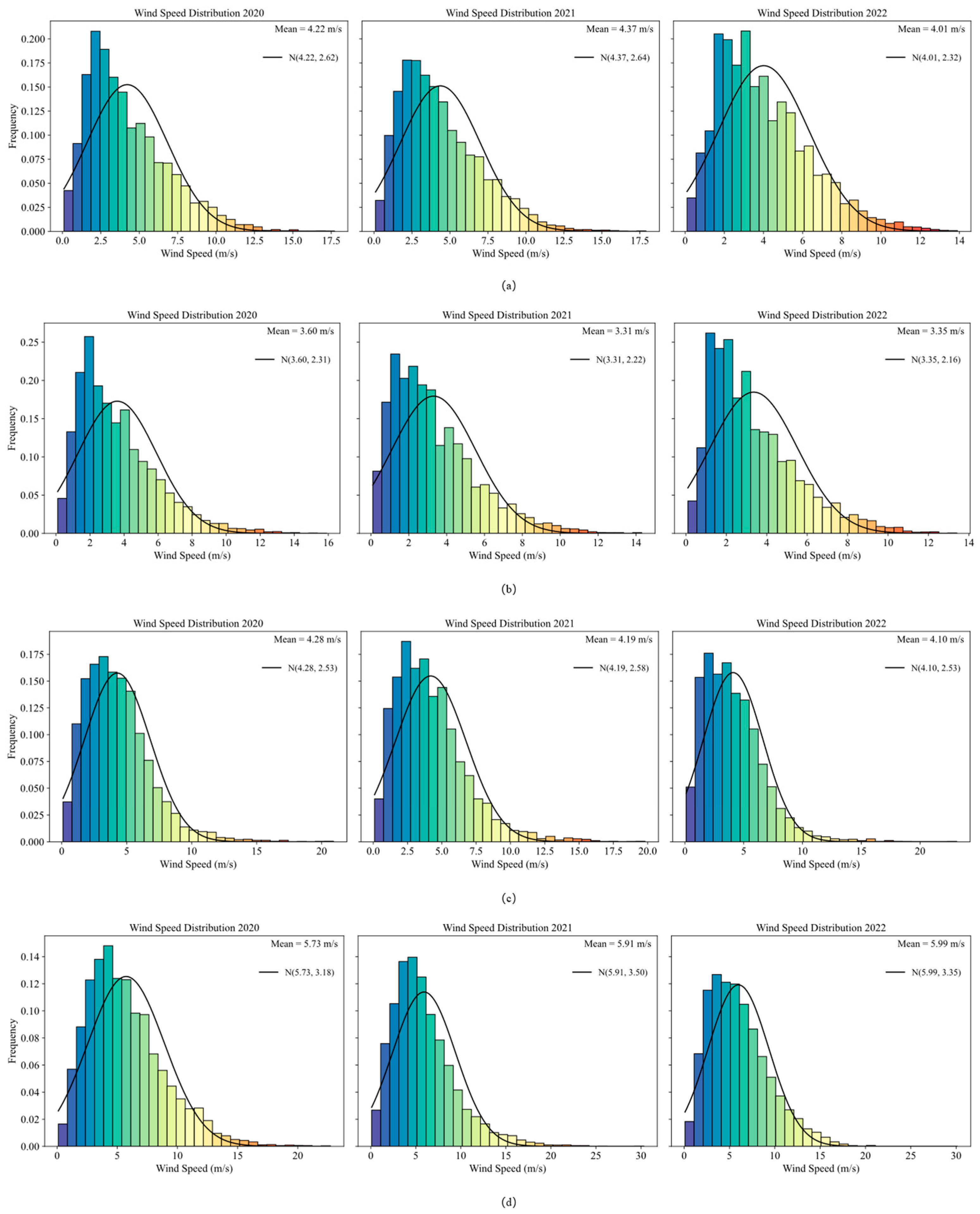
The wind frequency in LHT from 2019 to 2022 is shown in Figure 3a. The wind frequency in LHT from 2019 is shown in Figure 3a. In 2019, the mean wind speed was 4.09 m/s, with the most frequent wind speeds occurring between 1.75 and 3.5 m/s, indicating a relatively stable wind resource base. The dominant clustering near this range suggests limited variability, reflecting moderate but reliable wind conditions for small-scale wind energy development. In 2020, the mean wind speed is 4.22 m/s, with the highest frequency occurring between 2 and 3.5 m/s, indicating stable wind resources. In 2021, the average wind speed shows a slightly higher range of 4.37 m/s, but a similar dominant one 2–4 m/s, suggesting comparable wind energy potential. In contrast, 2022 records the lowest mean wind speed of 4.01 m/s, with prevailing speeds concentrated at 1.75–3.75 m/s, reflecting marginally weaker but still viable conditions.
The persistent clustering of frequent wind speeds near their respective annual means further confirms low interannual variability. These findings suggest that the region possesses reliably moderate wind resources, suitable for small-scale wind energy development with minimal year-to-year uncertainty.
The wind speed distribution at XCS from 2019 to 2022 is shown in Figure 3b. In 2019, the average wind speed was 3.39 m/s, with the highest frequency concentrated in the range of 1.5–3.75 m/s, suggesting a moderate and consistent wind profile. This distribution indicates that wind energy potential remains stable, providing sufficient conditions for continuous utilization. In 2020, the average wind speed was 3.60 m/s, with the most frequent wind speeds occurring between 2 and 4 m/s, indicating a moderate and consistent wind profile. The year 2021 recorded a slightly lower mean wind speed of 3.31 m/s and maintained a similar dominant range of 2–4 m/s, suggesting stable wind energy availability. In 2022, the mean wind speed slightly recovered to 3.35 m/s, with the highest frequencies again concentrated in the 2–4 m/s range, demonstrating continued consistency in wind behavior.
The wind speed distribution at ZFD from 2019 to 2022 is shown in Figure 3c. In 2019, the mean wind speed reached 4.31 m/s, with the most frequent wind speeds occurring between 2 and 5 m/s. This dominant range highlights steady wind availability, indicating the site’s suitability for wind exploitation under relatively consistent low-to-moderate wind regimes. In 2020, the average wind speed was 4.28 m/s, with the most frequent wind speeds occurring between 2 and 5 m/s. The year 2021 recorded a slightly higher mean wind speed of 4.19 m/s and maintained a similar dominant range of 0.5–4 m/s, suggesting stable wind energy availability in low wind speed areas. In 2022, the mean wind speed dropped to 4.10 m/s, with the highest frequencies concentrated in the 0.5–5 m/s range, demonstrating continued consistency in low wind speed behavior.
The long-term wind speed distribution at SSN from 2019 to 2022 is shown in Figure 3d. The average wind speed in 2019 was 5.25 m/s, with prevailing wind speeds concentrated in the 2.5–5.5 m/s range. The stable clustering around this band reflects robust and persistent wind conditions, supporting the potential for effective wind power generation. In 2020, the average wind speed was 5.73 m/s, with the most frequent wind speed occurring between 2.5 and 5.5 m/s. The year 2021 recorded a slightly higher mean wind speed of 5.91 m/s, maintaining a similar dominant range of 3–6 m/s. In 2022, the mean wind speed dropped to 5.99 m/s, with the highest frequencies again concentrated in the 3–6 m/s range, demonstrating continued consistency wind speed behavior.
The persistent peak frequencies across all four years, closely surrounding their respective annual means, highlight low interannual variability in wind conditions. This consistent wind profile indicates that the region offers reliably moderate wind energy potential, making it suitable for small- to medium-scale wind energy projects with low risk from year-to-year fluctuations. By contrasting four sites, SSN, the most south site, in south-east China possesses highest average wind speeds around 5.9 m/s, while XCS, the most north site, possess the least wind speeds due to the most complex terrain.

3. Example

3.1. Dataset Division and Seasonal Configuration

This chapter presents a comprehensive analysis of the BP-PSO hybrid model’s performance in wind speed forecasting across four coastal sites, focusing on its accuracy at annual and seasonal scales. The study evaluates the model’s ability to capture long-term wind patterns and seasonal variations, while also highlighting the spatial and temporal differences in forecasting outcomes.
The dataset was divided into training and testing phases to ensure robustness, with wind speed records spanning from January 2019 to December 2022. Data from January 2019 to December 2021 served as the training set, ensuring temporal diversity and covering multiple annual cycles. The testing set comprised data from 2022, which remained unseen during training to support independent evaluation.
Seasonal models were developed using calendar-based segmentation, with spring defined as March to May, summer as June to August, autumn was divided from September to November, and winter was defined as January, February, and December in 2022. Seasonal training datasets were constructed by extracting each season’s data from the 2019–2021 period, ensuring consistency across years. For example, the spring model was trained solely on March–May data from three consecutive years, following the same principle for other seasons. Two kinds of training data splitting methods are described in Figure 4.
This configuration enabled consistent comparison between a globally trained multi-year model and seasonally segmented models, while also clarifying the impact of season-specific characteristics on predictive accuracy. The results are contextualized within the broader framework of wind energy forecasting, emphasizing the importance of accurate predictions for renewable energy integration and grid management.
A widely used set of statistical indicators were employed to evaluate model performance, including Root Mean Square Error (RMSE), the coefficient of determination (R2), MAE (mean absolute error), NRMSE (Normalized Root Mean Square Error), RMSE_CI (RMSE Credit Interval), and Skill. RMSE quantifies the square root of the average squared differences between predicted and observed wind speeds, placing greater emphasis on larger errors. Lower RMSE values indicate higher predictive precision and model reliability. R2 measures the proportion of variance in observed wind speeds that can be explained by the model predictions. Higher R2 values, approaching unity, reflect stronger correlation and better model fit, confirming that the model effectively captures the variability of wind speed patterns. MAE is the average absolute difference between predictions and observations. RMSE_CI represents the 95% confidence interval of the RMSE, estimated via block bootstrap resampling, which quantifies the statistical uncertainty of the model’s prediction error. NRMSE quantifies the relative prediction error, obtained by normalizing RMSE by the mean wind speed, so that different datasets or scales can be compared. Skill measures the relative improvement of BP-PSO over the persistence baseline, computed as following formula:
s k i l l M o d e l a = 1 R M S E B P P S O R M S E M o d e l a

3.2. Multi-Year Forecast Model Performance

3.2.1. Multi-Year Forecast Outcome in LHT

The predicted and actual wind speeds using the BP-PSO model trained with multi-year datasets are compared in Figure 5 on the left. Overall, the model effectively captures wind speed variations, particularly in the 2–8 m/s range, where predictions closely match observed values. Accurate tracking is evident during spring and autumn, reflecting stable performance. However, slight underestimations occur at peaks above 10 m/s, and the model shows limited responsiveness at abrupt transitions. Despite these minor discrepancies, the overall agreement between predicted and measured series confirms the model’s robustness for long-term wind speed forecasting.
The error distribution of wind speed predictions based on the multi-year model is illustrated in Figure 5 on the right. The histogram exhibits a nearly symmetric, bell-shaped profile centered around zero, indicating the absence of significant systematic bias in the forecasts. Most errors are concentrated within the range of 2 m/s, suggesting that the model maintains stable predictive performance for most cases. While few larger deviations extending beyond 4 m/s are observed, their frequency is comparatively low, implying that extreme errors occur only occasionally. Overall, the error structure confirms that the model delivers consistent and unbiased predictions, with high reliability in capturing general wind speed dynamics.

3.2.2. Multi-Year Forecast Outcome in XCS

The comparison between predicted and observed wind speeds is illustrated in Figure 6 on the left. Overall, the model successfully tracks the temporal evolution of wind speeds across the study period. In the moderate range of 2–6 m/s, predicted values closely align with measured fluctuations, reflecting strong capability in reproducing gradual changes. During periods of stronger winds above 10 m/s, the amplitudes tend to be slightly underestimated, leading to minor deviations at peaks. While the model captures the timing of most transitions, it occasionally lags in representing abrupt surges, suggesting a limited responsiveness to sudden wind speed shifts.
The error distribution corresponding to these predictions is presented in Figure 6 on the right. The histogram shows a nearly symmetric shape centered around zero, which indicates the absence of systematic bias. Most of the deviations are confined within 3 m/s, confirming that the model provides stable accuracy under typical wind conditions. This distribution demonstrates that the model achieves consistent and unbiased forecasts, offering robust reliability for long-term wind speed prediction.

3.2.3. Multi-Year Forecast Outcome in ZFD

The comparison between predicted and actual wind speeds using the multi-year model is presented in Figure 7 on the left. The model generally reproduces the temporal variation in wind speeds throughout 2022, especially within the 3–10 m/s range, where predictions closely follow the observed dynamics. It effectively captures moderate fluctuations and seasonal changes. However, during extreme wind events above 15 m/s, the model tends to underestimate peak magnitudes, and at abrupt transitions the response is sometimes delayed, indicating limited accuracy in extreme conditions.
The corresponding error distribution is shown in Figure 7 on the right. The histogram exhibits a sharp peak centered around zero, confirming the absence of significant systematic bias. Most prediction errors are within 5 m/s, suggesting stable and consistent forecast performance.

3.2.4. Multi-Year Forecast Outcome in SSN

The comparison between predicted and actual wind speeds using the multi-year BP-PSO model is illustrated in Figure 8 on the right. Overall, the model effectively captures the temporal evolution of wind speeds throughout 2022, with close agreement in the 3–12 m/s range where most wind events occur. Moderate and gradual fluctuations are reproduced well, while discrepancies appear at sharp peaks above 15 m/s, where the model tends to underestimate extreme values. At transition points, predictions generally follow observed variations, though occasional lag is evident during rapid changes.
The error distribution is presented in Figure 8 on the right. The histogram exhibits a sharp, symmetric peak centered near zero, suggesting the absence of systematic bias in forecasts. Most errors lie within ±3 m/s, reflecting stable accuracy under normal wind conditions. Although a few larger deviations beyond ±5 m/s are observed, their frequency is low, confirming that the model provides consistent and reliable long-term wind speed predictions.

3.3. Seasonal Model Performance

3.3.1. Seasonal Forecast Outcome in LHT

The seasonal forecasts are presented in Figure 9, representing spring, summer, autumn, and winter predictions, respectively. Overall, the seasonal BP-PSO models demonstrate improved alignment with observed wind speed patterns compared to the multi-year model, showing enhanced responsiveness to intra-annual variability.
Winter forecast results are shown in Figure 9. The winter prediction closely aligns with measured values across a wide spectrum of wind speeds, effectively capturing both gradual changes and sudden transitions. Peak tracking is notably improved compared to other seasons, particularly during events above 10 m/s. This suggests that the winter dataset, characterized by stronger variability and higher wind magnitudes, enhances the model’s capacity to generalize extreme behaviors.
Spring forecast illustrates that the spring-only prediction effectively tracks moderate wind events, especially in the 2–7 m/s range. The seasonal progression is well reproduced, though the model occasionally lags during sharp increases, resulting in a slight underestimation of extreme events. The overall profile is smooth, indicating stable prediction but limited adaptability to sudden accelerations due to the relatively low variability in spring winds.
The summer prediction shows stronger consistency with the actual data, both in amplitude and phase. The model successfully captures multiple sharp transitions and higher peaks, demonstrating improved responsiveness to short-term variability. Minor underestimations occur at very high frequencies, but the richer variability of summer winds contributes to enhanced peak detection compared to spring.
The autumn model replicates observed wind speeds with high accuracy in the 3–9 m/s range, maintaining good stability. However, during extreme wind events above 12 m/s, the predicted values are slightly suppressed, showing that the model tends to smooth abrupt transitions. Despite this, autumn predictions exhibit balanced performance between stability and peak responsiveness.
Collectively, the seasonal BP-PSO models demonstrate robust predictive skill across all seasons, with enhanced sensitivity to short-term fluctuations and peak wind events. Among them, the summer and winter models show superior responsiveness to extremes, while spring and autumn emphasize smoother stability. These findings highlight the advantage of seasonal-focused training in improving prediction accuracy and adaptability to intra-annual wind dynamics.
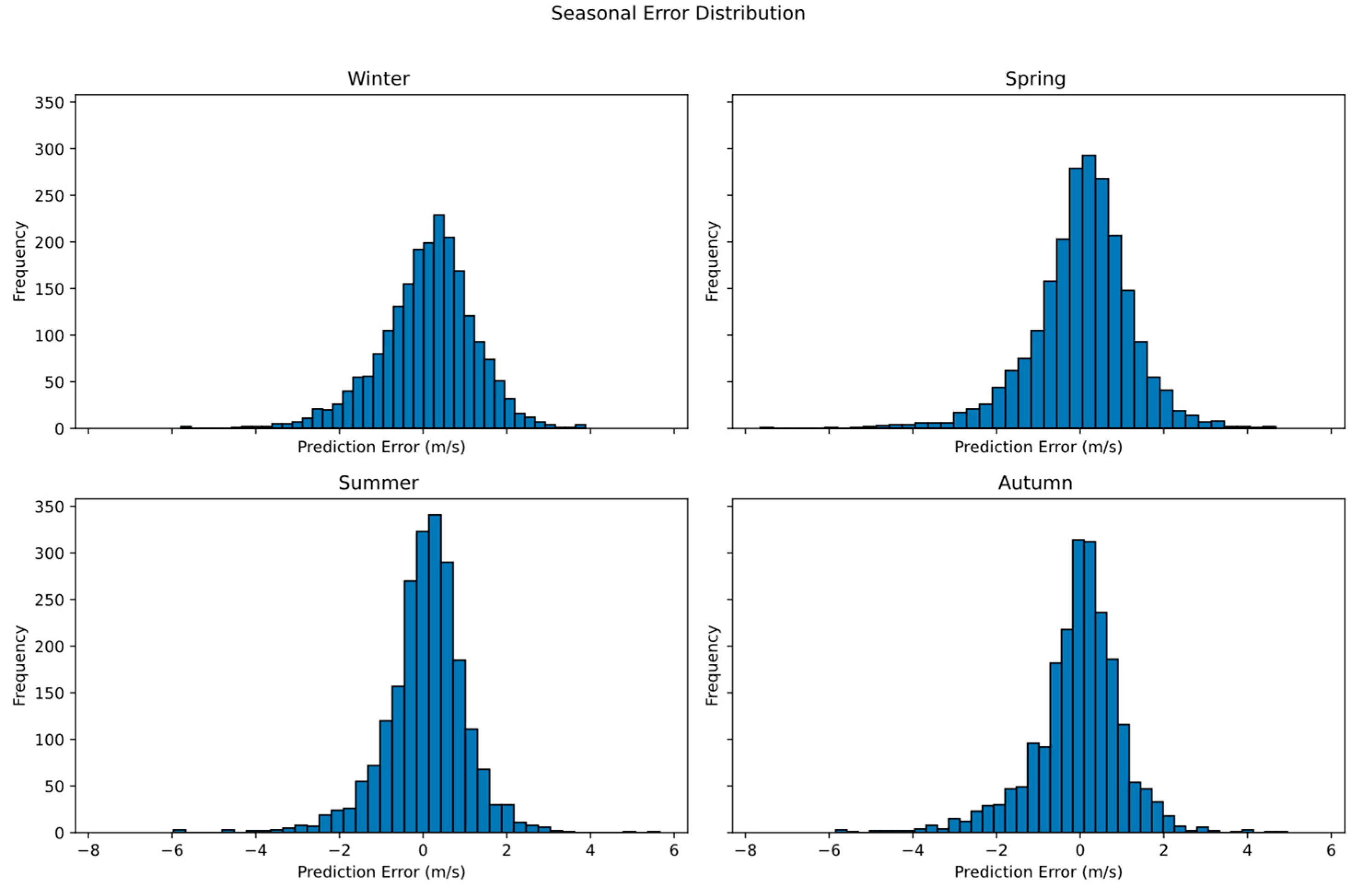
The seasonal error distributions are shown in Figure 10. In spring, errors cluster tightly around zero, indicating stable prediction but with a tendency to slightly suppress extremes. Summer exhibits broader dispersion, reflecting improved sensitivity to variability but at the cost of occasional large deviations. Autumn errors remain relatively symmetric and narrow, highlighting consistent performance across moderate wind regimes. Winter shows the widest distribution, with both under- and over-predictions at high magnitudes, implying that while the model effectively engages strong winds, it also faces greater difficulty in constraining extremes. Collectively, these results demonstrate that seasonal specialization enhances adaptability, though the trade-off between peak responsiveness and error stability differs across seasons.

3.3.2. Seasonal Forecast Outcome in XCS

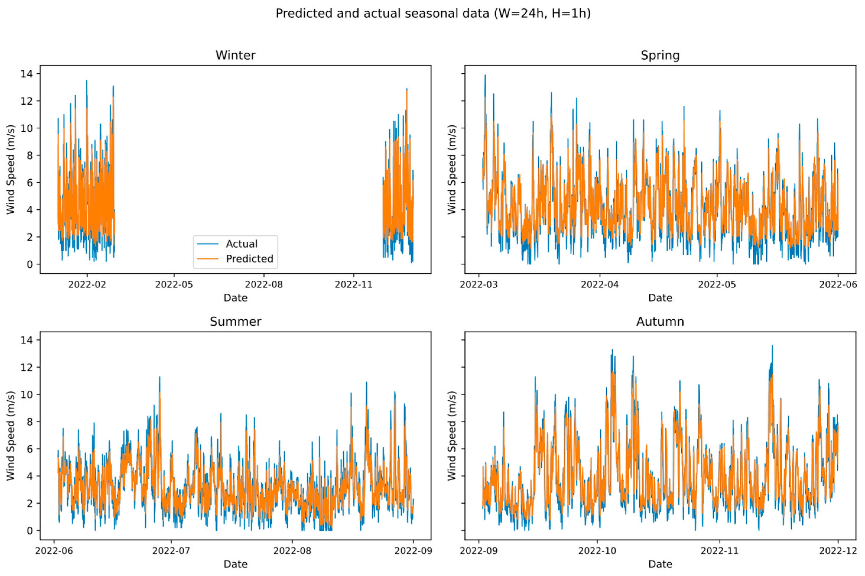
The seasonal forecasts at the selected site are presented in Figure 11, illustrating that the BP-PSO model achieves varying levels of accuracy across spring, summer, autumn, and winter.
In the winter-only prediction, the model demonstrates the highest predictive skill across a wide range of wind speeds. Both moderate and strong winds above 10 m/s are captured with high fidelity, and abrupt transitions are well reproduced. Although a few extreme peaks remain slightly underestimated, the results highlight the model’s enhanced capability under the more dynamic and variable winter wind regime.
In the spring-only prediction, the model reproduces the seasonal evolution of wind speeds primarily within the 3–8 m/s range with reasonable accuracy. While gradual fluctuations are well captured, the predictions tend to smooth abrupt increases, resulting in slight underestimation during rapid acceleration phases. This reflects the relatively limited variability of spring winds, which constrains the model’s sensitivity to sudden transitions.
In the summer-only prediction, the agreement between forecasts and observations improves noticeably. The model accurately follows both the timing and amplitude of wind speed changes, including sharper rises above 8 m/s. Although some high-frequency oscillations are smoothed, the model exhibits stronger adaptability to the richer variability and higher peaks characteristic of summer winds.
In the autumn-only prediction, the forecasts maintain stable accuracy in the 4–9 m/s range, where most wind events are concentrated. Gradual variations are effectively tracked, but peaks exceeding 12 m/s are underestimated, indicating that autumn predictions prioritize overall stability at the expense of responsiveness to extremes.
The seasonal error history is illustrated in Figure 12. In spring, errors are concentrated closely around zero, indicating stable forecasts with minor deviations but limited responsiveness to sudden wind fluctuations. Summer errors display a broader spread, suggesting that while the model adapts better to higher variability, it occasionally produces larger over- or underestimations. Autumn errors return to a narrower distribution, reflecting consistent accuracy across moderate wind ranges, though peak events remain slightly underestimated. Winter shows the widest error dispersion, particularly under strong wind conditions, highlighting the difficulty of capturing extremes. Nevertheless, the distribution remains nearly symmetric about zero, confirming the absence of systematic bias. Collectively, these results emphasize a seasonal trade-off between forecast stability and adaptability, with winter achieving the greatest variability but also facing the largest prediction challenges.

3.3.3. Seasonal Forecast Outcome in ZFD

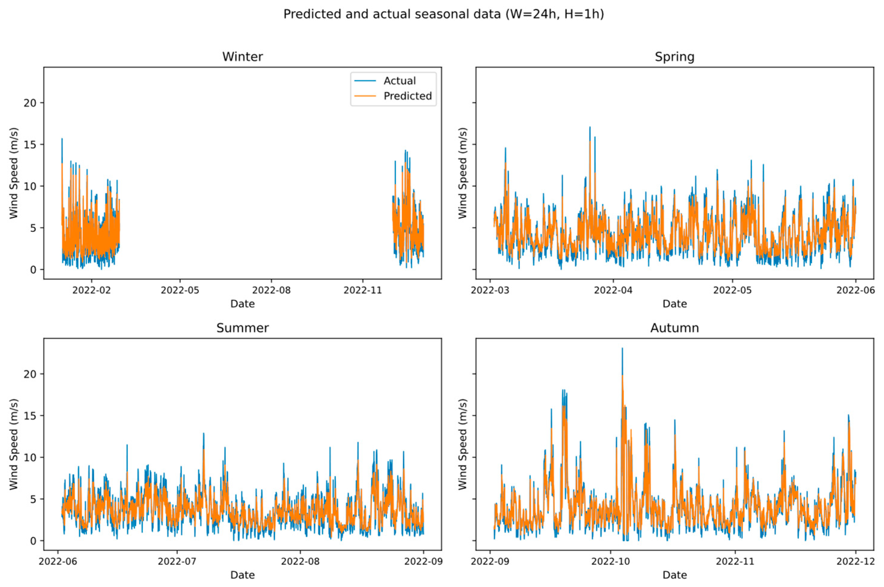
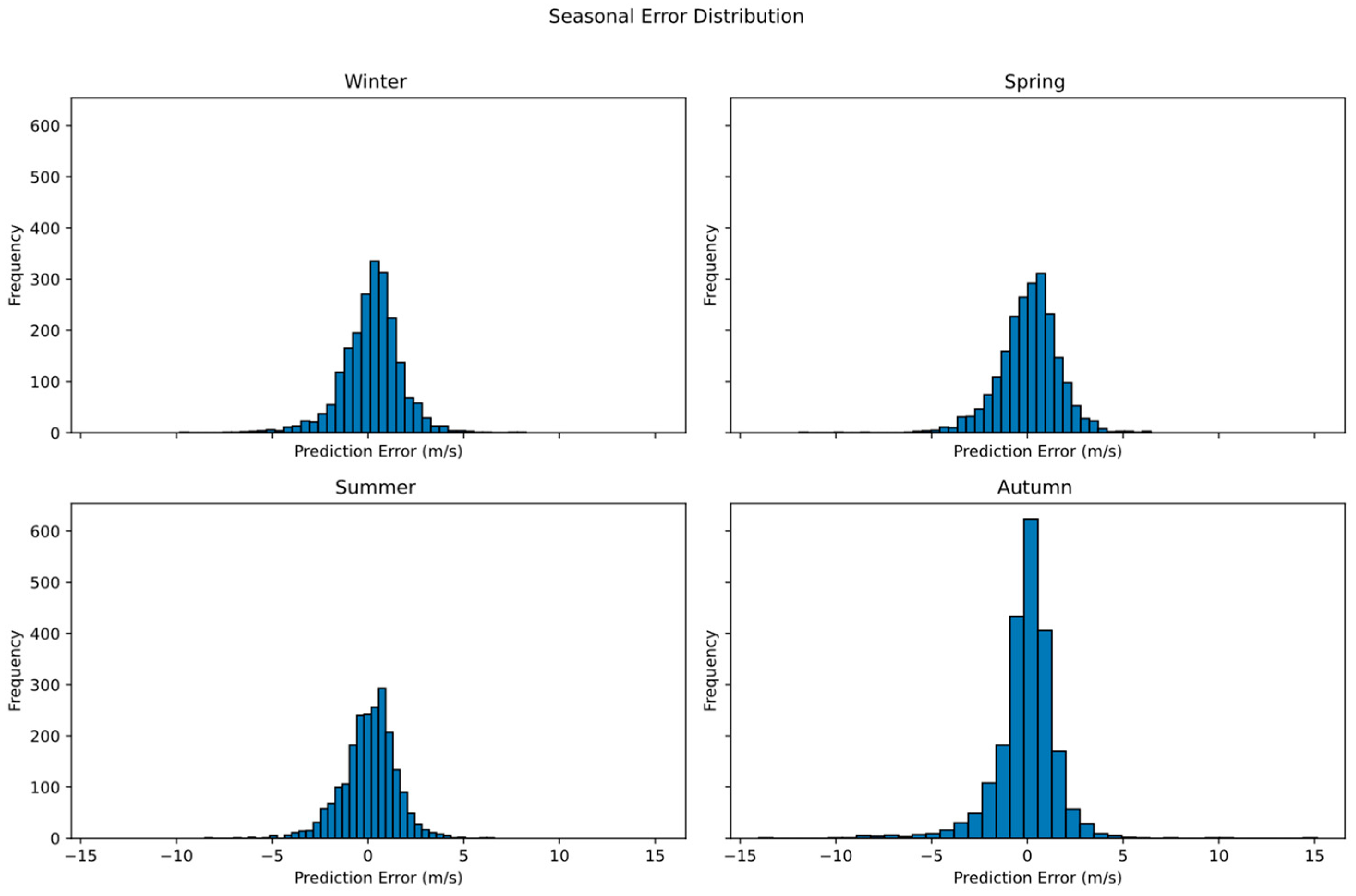
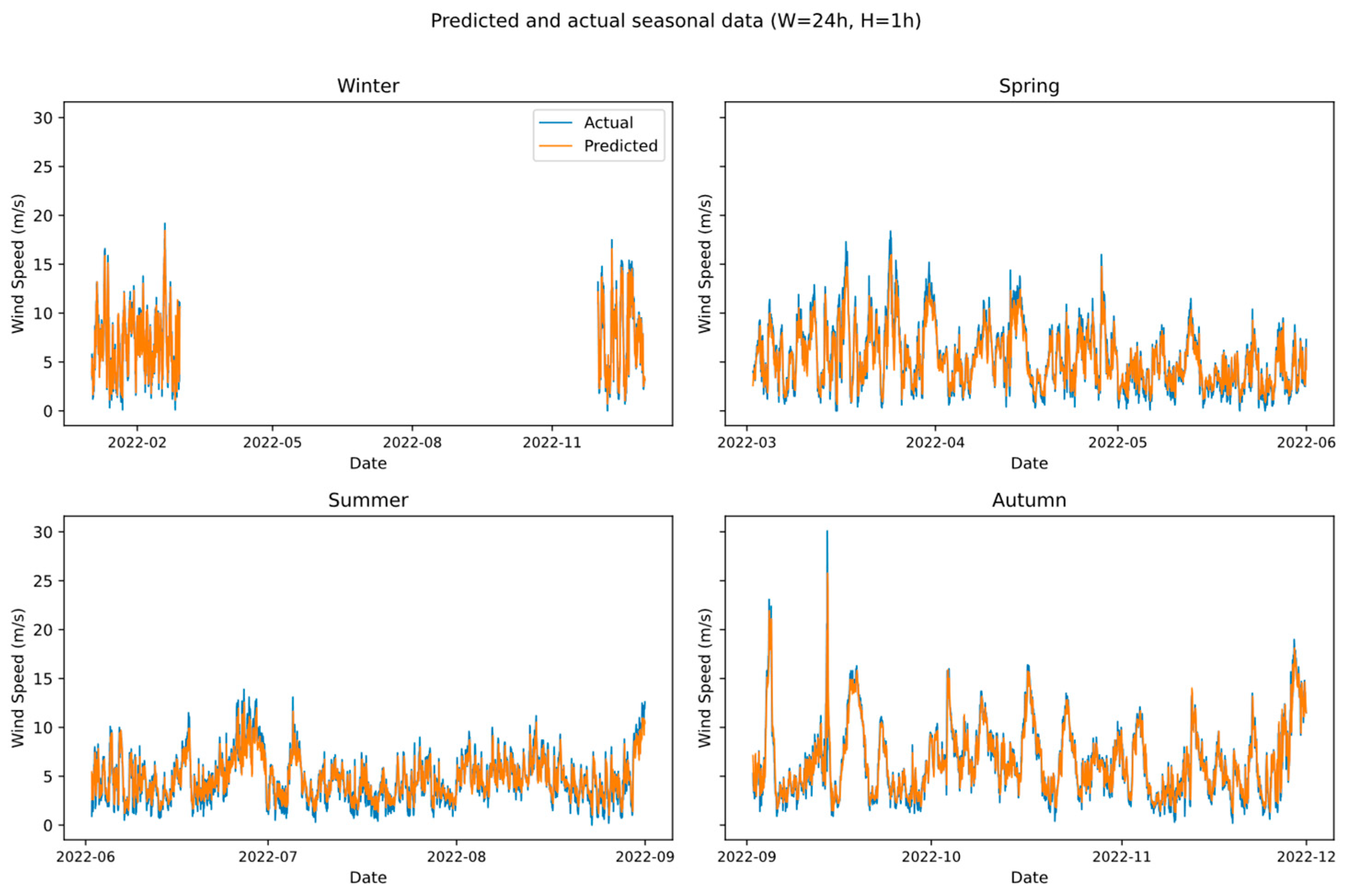
The seasonal forecasts at ZFD are presented in Figure 13, showing that the BP-PSO model achieves reasonable accuracy across all seasons with some seasonal variability in performance.
In the winter prediction model, the winter forecasts display the best overall performance, effectively capturing both moderate and strong winds. Predictions align well with observed values across a wide range, and high wind events above 10 m/s are reproduced more accurately than in other seasons. Although some peak magnitudes are underestimated, the winter dataset provides greater variability that enhances the model’s capability to resolve extremes.
In the spring prediction model, the model effectively tracks moderate wind speeds in the 2–7 m/s range, capturing seasonal evolution with relatively stable alignment. However, abrupt transitions are slightly smoothed, leading to underestimation of short-lived high peaks, reflecting limited adaptability to sudden accelerations in spring winds.
In the summer prediction model, forecasts show stronger agreement with observations, particularly in reproducing multiple sharp fluctuations and higher peaks above 8 m/s. While the model occasionally smooths high-frequency oscillations, its responsiveness to stronger variability is superior to spring, suggesting that the richer summer dataset improves adaptability to transient events.
In the autumn prediction model, the model delivers consistent predictions, with close alignment in the 3–8 m/s range. Gradual changes are well captured, but wind events exceeding 12 m/s are partially suppressed, indicating that the model emphasizes stability over extreme responsiveness during this season.
The errors in histograms for ZFD are shown in Figure 14. Spring and autumn errors are narrowly clustered around zero, suggesting stable forecasts but a tendency to smooth sharp changes. Summer errors are broader, reflecting greater sensitivity to variability yet occasional larger deviations. Winter displays the widest spread, with both under- and overestimation at strong winds, but the overall symmetry indicates the absence of systematic bias.

3.3.4. SSN

The seasonal predictions are shown in Figure 15, illustrating the model’s ability to reproduce wind speed variability under different seasonal conditions.
The spring forecast results track moderate wind speeds in the 2–7 m/s range with overall stability. Gradual variations are well captured, but sharp increases are slightly underestimated, suggesting limited adaptability to sudden accelerations due to the relatively low variability of spring winds.
The summer forecast results are predicted to exhibit stronger agreement with observations, effectively replicating both the timing and amplitude of multiple wind events. Peaks above 8 m/s are captured more faithfully than in spring, though occasional smoothing of rapid oscillations remains, leading to minor underestimation of extremes.
The autumn forecast results demonstrate consistent alignment within the 3–8 m/s range. It performs well in tracking seasonal progression, though wind events exceeding 12 m/s tend to be suppressed. This indicates that while autumn forecasts emphasize stability, they are less sensitive to transient extreme conditions.
The winter forecast results deliver the most robust performance, successfully capturing both gradual changes and strong wind fluctuations. High wind events above 10 m/s are represented more accurately than in other seasons, although some peak magnitudes are still slightly underestimated. The greater variability of winter winds enhances the model’s capacity to generalize extreme dynamics.
The error distributions are illustrated in Figure 16. Spring and autumn errors are narrowly centered around zero, reflecting stable but somewhat smoothed forecasts. Summer errors broaden, showing greater responsiveness to variability with occasional larger deviations. Winter exhibits the widest spread, with both under- and overestimation at strong winds, yet the symmetric distribution suggests no systematic bias.

3.4. Forecast Time Series and Prediction Interval

The panel in Figure 17 presents the one-hour-ahead predictions of wind speed for 2022 at the following four monitoring sites: LHT (top-left), XCS (top-right), ZFD (bottom-left), and SSN (bottom-right). In each subplot the bold solid line indicates the observed values, the thinner line the model’s mean forecast, and the shaded region the 90% prediction interval.
Across all sites, the prediction intervals successfully capture most of the observed fluctuations, demonstrating the model’s calibrated uncertainty quantification. The variation in interval width between sites reflects differing local dynamics and model confidence: for example, SSN shows wider intervals (indicating larger variability or lower certainty), whereas LHT exhibits narrower bands, pointing to more stable forecast conditions. Together, these results illustrate that our BP-PSO framework yields not only accurate mean forecasts but also reliable probabilistic bounds in operational, multi-site wind speed prediction.

3.5. Results Analysis

Table 4 summarizes the prediction errors across four sites (LHT, XCS, ZFD, SSN) under multi-year and seasonal training datasets, evaluated by RMSE, R2, MAE, NRMSE, skills scores relative to persistence and ARIMA baselines, and RMSE_CI.
Overall, XCS exhibits the lowest prediction errors and highest correlation, with RMSE values below 1.2 m/s in all seasons and an average R2 of 0.81, indicating a relatively stationary wind regime and high model generalizability. LHT and SSN show moderate and stable accuracy, with RMSE clustered around 1.27–1.30 m/s and R2 above 0.70; SSN performs particularly well in winter (R2 = 0.884, NRMSE = 0.165), reflecting a smoother seasonal pattern and higher forecast reliability. In contrast, ZFD consistently yields the largest errors (RMSE ≈ 1.54 m/s, R2 ≈ 0.63), especially in autumn, where strong turbulence and complex terrain effects increase forecast uncertainty.
Across sites, the BP-PSO model achieves positive skill scores against persistence (4–6%) and substantial improvements over ARIMA, confirming its robustness across both smooth and highly variable regimes. The inter-site comparison further reveals that XCS and SSN are the most predictable stations, while ZFD represents the most challenging environment for short-term wind speed forecasting due to intensified local variability.
The comparative performance of different models across four sites is illustrated in Figure 18, evaluated using RMSE, R2, and MAE. For LHT, the summer model achieves the lowest RMSE and MAE, indicating the most accurate prediction, while the spring model records the highest RMSE with a lower R2, reflecting weaker performance. At XCS, the summer and autumn models perform best, combining low RMSE/MAE with R2 values exceeding 0.80, whereas the spring model is less accurate with elevated RMSE/MAE and reduced R2. For ZFD, the following clear discrepancies are observed: the summer model yields the lowest RMSE and MAE, whereas the autumn model performs the worst, with the highest RMSE/MAE and depressed R2, indicating greater variability. In contrast, SSN demonstrates stable behavior across all models, with the winter model achieving the best performance (lowest RMSE/MAE and highest R2), while the spring model shows slightly higher errors. Overall, seasonal differences are most pronounced at ZFD, while XCS and SSN exhibit more consistent predictive accuracy across seasonal and multi-year models.
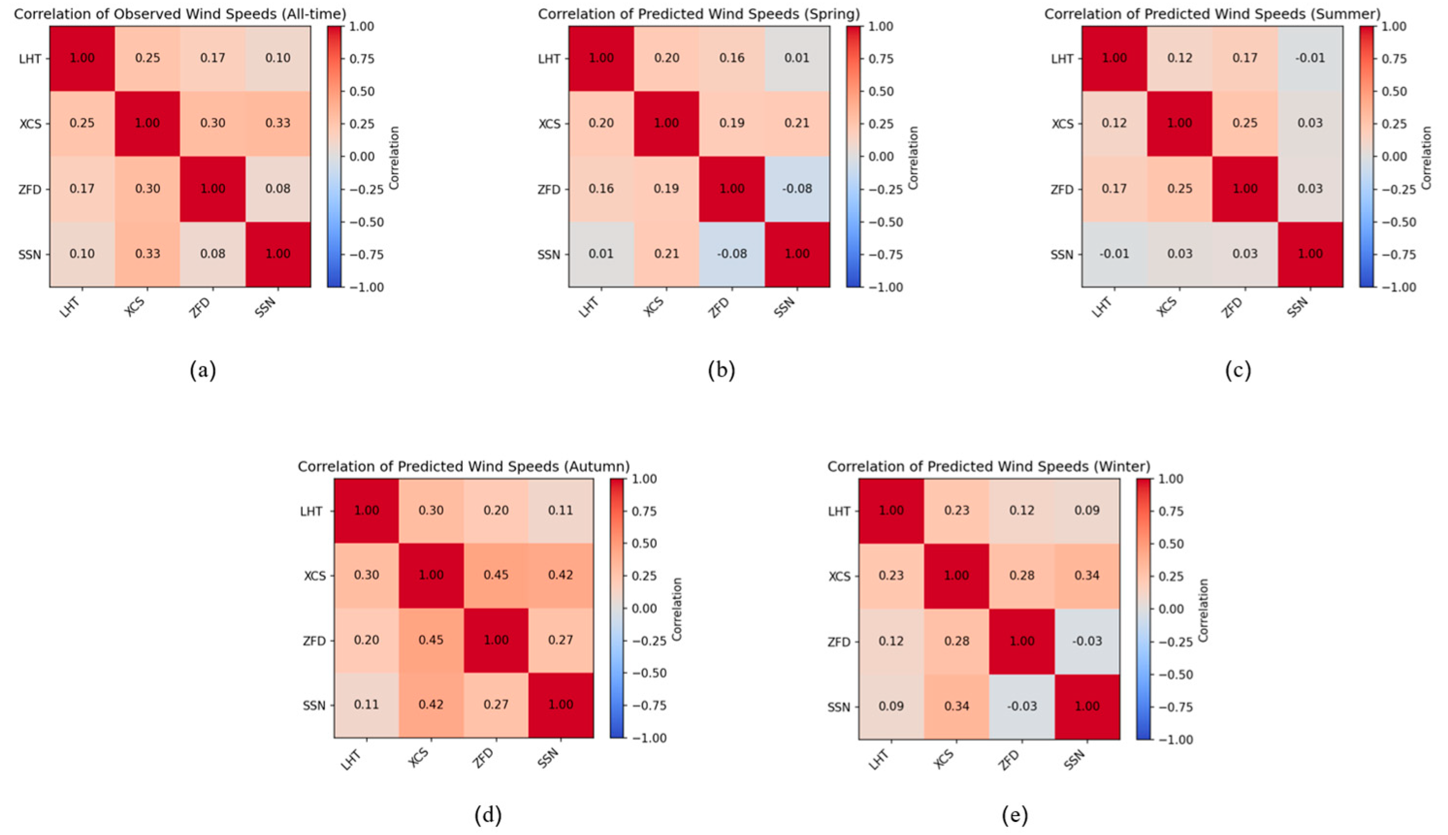
Figure 19 presents the correlation analysis of predicted wind speeds across the four stations under five training strategies as follows: (a) multi-year, (b) spring, (c) summer, (d) autumn, and (e) winter. The multi-year model (a) yields the most stable and generally higher correlations, particularly between ZFD and XCS, rating to 0.3. Seasonal models such as spring and summer show weak correlation, with the rates below 0.25. However, in autumn (d) the degree of correlation increases especially between northern sites, ZFD and XCS (0.45), XCS and SSN (0.42) and XCS and LHT (0.3). The winter model (e) achieves some of the highest cross-station correlations, with values between SSN and XCS stations, suggesting that winter wind regimes share broader consistency across geographically distinct regions. Collectively, these results highlight that multi-year and winter-trained models achieve the strongest inter-station correlations, while summer and autumn predictions exhibit larger spatial divergence. Figure 19 indicates that inter-site wind speed correlations strengthen when synoptic scale forcing and seasonal cycles dominate but weaken where local coastal effects phases exist. Although XCS and SSN are far apart, their moderate correlation likely reflects shared exposure to the same prevailing monsoonal/northerly flow and coastal pressure gradient patterns during the analyzed period.
Firstly, when considering all three error indicators together—RMSE, MAE, and R2—the multi-year models at LHT, XCS, and SSN deliver the most balanced and reliable performance. Their RMSEs range from 1.091 to 1.273 m/s, MAEs from 0.792 to 0.951 m/s, and R2 values remain above 0.70, peaking at 0.854 at SSN. This improvement arises from the richer multi-year training data, which smooths out seasonal noise and enhances generalization. In contrast, the autumn model at ZFD performs the worst overall, exhibiting the highest RMSE (1.641 m/s) and the lowest R2 (0.697), confirming that increased turbulence and seasonal variability during autumn in the Bohai region led to reduced forecast accuracy.
Secondly, among the three Bohai Bay stations (LHT, XCS, ZFD), the error indicators display similar seasonal trends. At all three sites, spring forecasts tend to show slightly higher RMSE and MAE than winter or summer, while the multi-year model improves overall stability. The consistent seasonal performance across these nearby coastal stations reflects shared meteorological forcing—particularly the seasonal transition of monsoon and sea–land thermal contrast—that shapes wind field variability in the Bohai area.
Thirdly, at SSN in Zhejiang Province, despite its greater geographical separation from the Bohai Bay cluster, the model maintains comparably low errors, with RMSE between 1.161 and 1.382 m/s, MAE between 0.883 and 1.066 m/s, and R2 consistently above 0.74, peaking at 0.886 in winter. The close alignment of these metrics with northern sites demonstrates that the BP-PSO framework exhibits strong spatial adaptability, capable of transferring predictive skill across distinct climatic zones and underlying coastal dynamics.
In summary, the multi-year configuration yields the most robust and consistent results across all stations, whereas the autumn model at ZFD represents the least reliable case. The coherence of seasonal behavior among the Bohai Bay sites and the steady performance at SSN together confirm both the regional stability and the broad geographical generalization capability of the proposed BP-PSO modeling approach.

4. Conclusions

Accurate wind speed forecasting remains vital for optimizing coastal wind energy utilization and operational strategies. This study evaluated the performance of multi-year and seasonal BP-PSO models across four coastal stations in China, spanning Bohai Bay in the north (LHT, XCS, ZFD) to Zhejiang Province in the south (SSN). Both modeling strategies exhibited strong generalization across time and space, demonstrating that BP-PSO can adapt effectively to diverse climatic conditions.
From a performance standpoint, the two model settings produced broadly comparable results, with RMSE values consistently within acceptable margins. At LHT and SSN, prediction errors of multi-year and seasonal models were nearly indistinguishable, with RMSEs ranging between 1.164 and 1.395 and 1.172 to 1.438, respectively, underscoring the stability of the framework under different temporal settings. At ZFD, however, seasonal errors were relatively higher, particularly in autumn, where RMSEs rose to 1.641, accompanied by lighter R2 values. These discrepancies reflect the influence of enhanced turbulence, convection, and localized atmospheric instabilities in coastal climates. Such findings suggest that multi-year training provides more robust long-term representation, whereas seasonal models enhance sensitivity to short-term dynamics.
Despite their relatively larger RMSEs, seasonal models offer computational advantages. Their narrower training windows and reduced dependence on extended historical data allow faster execution, making them suitable for adaptive or real-time forecasting scenarios. The observed trade-off between accuracy and efficiency indicates that seasonal models are appropriate for operational contexts requiring rapid updates, while multi-year models remain preferable for strategic assessments. Seasonal comparisons further confirmed that winter forecasts achieved higher accuracy, benefiting from broader variability, whereas autumn at ZFD posed the greatest challenge, reflecting site-specific dynamics.
A notable outcome is the consistent performance at SSN, a station geographically distant from Bohai Bay. Despite climatic differences, SSN maintained RMSEs between 1.172 and 1.438 and R2 values above 0.735, peaking at 0.884. The ability of the BP-PSO framework to sustain accuracy across distinct northern and southeastern coastal climates highlights its strong spatial adaptability. This transferability is particularly valuable for large-scale coastal wind assessments in regions with limited monitoring coverage.
In conclusion, both multi-year and seasonal BP-PSO models deliver reliable wind speed forecasts with complementary strengths. Multi-year models provide slightly higher accuracy and long-term stability, while seasonal models ensure computational efficiency and adequate precision for short-term applications. These results confirm BP-PSO as a practical and robust approach for wind forecasting and coastal energy evaluation in China.
Looking ahead, incorporating additional meteorological datasets (e.g., reanalysis, satellite products) and adopting multi-station fusion methods may further enhance spatial robustness. Moreover, developing adaptive weighting mechanisms and automated preprocessing pipelines could reduce manual intervention and improve scalability. Such advances will help establish more intelligent forecasting systems, supporting the sustainable growth of coastal wind energy.

Author Contributions

Conceptualization, S.J., J.J. and S.D.; Methodology, S.J. and S.D.; Investigation, S.J.; Data curation, S.J.; Writing—original draft, S.J.; Writing—review & editing, J.J. and S.D.; Supervision, J.J.; Project administration, J.J. and S.D.; Funding acquisition, J.J. and S.D. All authors have read and agreed to the published version of the manuscript.

Funding

This work was supported by the National Key R&D Program of China—Intergovernmental International Scientific and Technological Innovation and Cooperation Program (Grant No. 2023YFE0115400), the Shanghai Pujiang Program (Grant No. 22PJ1421200 and No. 22PJ1411400).

Institutional Review Board Statement

Not applicable.

Informed Consent Statement

Not applicable.

Data Availability Statement

The data presented in this study are available on request from the corresponding author.

Acknowledgments

Thanks to the National Science and Technology Resource Sharing Service Platform—National Marine Science Data Center (https://mds.nmdis.org.cn, accessed on 1 June 2025) for providing data.

Conflicts of Interest

The authors declare no conflict of interest.

Abbreviations

The following abbreviations are used in this manuscript:
BPBack propagation
PSOParticle swarm optimization
LHTLao Hu Tan
XCSXiao Chang Shan
ZFDZhi Fu Dao
SSNShen Shan
RMSERoot Mean Square Error
NRMSEStandard deviation
MAEMean absolute error
NRMSENormalized Root Mean Square Error
RMSE_CIRoot Mean Square Error Credit Interval

References

  1. Desalegn, B.; Gebeyehu, D.; Tamrat, B.; Tadiwose, T.; Lata, A. Onshore versus offshore wind power trends and recent study practices in modeling of wind turbines’ life-cycle impact assessments. Clean. Eng. Technol. 2023, 17, 100691. [Google Scholar] [CrossRef]
  2. Li, J.; Wang, G.; Li, Z.; Yang, S.; Chong, W.T.; Xiang, X. A review on development of offshore wind energy conversion system. Int. J. Energy Res. 2020, 44, 9283–9297. [Google Scholar] [CrossRef]
  3. Global Wind Energy Council. Global Wind Report 2023; GWEC: Brussels, Belgium, 2023. [Google Scholar]
  4. Ahmed, S.D.; Al-Ismail, F.S.M.; Shafiullah, M.; Al-Sulaiman, F.A.; El-Amin, I.M. Grid integration challenges of wind energy: A review. IEEE Access 2020, 8, 10857–10878. [Google Scholar] [CrossRef]
  5. REN21. Renewables 2023 Global Status Report Collection; Report Citation: REN21; REN21: Paris, France, 2023. [Google Scholar]
  6. Wang, X.; Shne, X.; Ai, X.; Li, S. Short-term wind speed forecasting based on a hybrid model of ICEEMDAN, MFE, LSTM and informer. PLoS ONE 2023, 18, e0289161. [Google Scholar]
  7. Yousuf, M.U.; Al-Bahadly, I.; Avci, E. Short-term wind speed forecasting based on hybrid MODWT-ARIMA-Markov model. IEEE Access 2021, 9, 79695–79711. [Google Scholar] [CrossRef]
  8. Clifton, A.; Smith, A.; Fields, M. Wind Plant Preconstruction Energy Estimates. Current Practice and Opportunities; National Renewable Energy Lab (NREL): Golden, CO, USA, 2016. [Google Scholar]
  9. Dhiman, H.S.; Deb, D. A review of wind speed and wind power forecasting techniques. arXiv 2020, arXiv:2009.02279. [Google Scholar] [CrossRef]
  10. Han, Y.; Mi, L.; Shen, L.; Cai, C.; Liu, Y.; Li, K.; Xu, G. A short-term wind speed prediction method utilizing novel hybrid deep learning algorithms to correct numerical weather forecasting. Appl. Energy 2022, 312, 118777. [Google Scholar] [CrossRef]
  11. Meenal, R.; Michael, P.A.; Pamela, D.; Rajasekaran, E. Weather prediction using random forest machine learning model. Indones. J. Electr. Eng. Comput. Sci. 2021, 22, 1208–1215. [Google Scholar] [CrossRef]
  12. Ren, C.; An, N.; Wang, J.; Li, L.; Hu, B.; Shang, D. Optimal parameters selection for BP neural network based on particle swarm optimization: A case study of wind speed forecasting. Knowl.-Based Syst. 2014, 56, 226–239. [Google Scholar] [CrossRef]
  13. Acikgoz, H.; Korkmaz, D. Short-term offshore wind speed forecasting approach based on multi-stage decomposition and deep residual network with self-attention. Eng. Appl. Artif. Intell. 2025, 146, 110313. [Google Scholar] [CrossRef]
  14. Li, Q.; Wang, G.; Wu, X.; Gao, Z.; Dan, B. Arctic short-term wind speed forecasting based on CNN-LSTM model with CEEMDAN. Energy 2024, 299, 131448. [Google Scholar] [CrossRef]
  15. Zhong, X.; Du, F.; Chen, L.; Wang, Z.; Li, H. Investigating transformer-based models for spatial downscaling and correcting biases of near-surface temperature and wind-speed forecasts. Q. J. R. Meteorol. Soc. 2024, 150, 275–289. [Google Scholar] [CrossRef]
  16. Wang, Z.; Ying, Y.; Kou, L.; Ke, W.; Wan, J.; Yu, Z.; Liu, H.; Zhang, F. Ultra-short-term offshore wind power prediction based on PCA-SSA-VMD and BiLSTM. Sensors 2024, 24, 444. [Google Scholar] [CrossRef]
  17. Wang, J.; Liu, X.Y.; Deng, E.; Ni, Y.-Q.; Chan, P.-W.; Yang, W.-C.; Tan, Y.-K. Acceleration and Reynolds effects of crosswind flow fields in gorge terrains. Phys. Fluids 2023, 35, 085143. [Google Scholar] [CrossRef]
  18. Zhao, Y. Research and application on BP neural network algorithm. In International Industrial Informatics and Computer Engineering Conference; Atlantis Press: Dordrecht, The Netherlands, 2015; pp. 1444–1447. [Google Scholar]
  19. Qu, Z.; Mao, W.; Zhang, K.; Zhang, W.; Li, Z. Multi-step wind speed forecasting based on a hybrid decomposition technique and an improved back-propagation neural network. Renew. Energy 2019, 133, 919–929. [Google Scholar] [CrossRef]
  20. Viet, D.T.; Phuong, V.V.; Duong, M.Q.; Tran, Q.T. Models for short-term wind power forecasting based on improved artificial neural network using particle swarm optimization and genetic algorithms. Energies 2020, 13, 2873. [Google Scholar] [CrossRef]
  21. Zhang, Y.; Chen, B.; Zhao, Y.; Pan, G. Wind speed prediction of IPSO-BP neural network based on lorenz disturbance. IEEE Access 2018, 6, 53168–53179. [Google Scholar] [CrossRef]
  22. Wang, Z.; Wang, B.; Liu, C.; Wang, W. Improved BP neural network algorithm to wind power forecast. J. Eng. 2017, 2017, 940–943. [Google Scholar] [CrossRef]
  23. Bagherpoor, T.; Kazemi Sormoli, S. Forecasting wind speed in Zabol city: A comparative study of CNN, LSTM, and CNN-LSTM models. Agric. Environ. Soc. 2024, 4, 95–107. [Google Scholar]
  24. Tsai, W.C.; Hong, C.M.; Tu, C.S.; Lin, W.M.; Chen, C.H. A review of modern wind power generation forecasting technologies. Sustainability 2023, 15, 10757. [Google Scholar] [CrossRef]
  25. Hanifi, S.; Lotfian, S.; Zare-Behtash, H.; Cammarano, A. Offshore wind power forecasting—A new hyperparameter optimisation algorithm for deep learning models. Energies 2022, 15, 6919. [Google Scholar] [CrossRef]
  26. Arrieta-Prieto, M.; Schell, K.R. Spatially transferable machine learning wind power prediction models: V− logit random forests. Renew. Energy 2024, 223, 120066. [Google Scholar] [CrossRef]
  27. Hadjoudj, Y.; Pandit, R. A review on data-centric decision tools for offshore wind operation and maintenance activities: Challenges and opportunities. Energy Sci. Eng. 2023, 11, 1501–1515. [Google Scholar] [CrossRef]
  28. Yang, H.; Tang, J.; Shao, W.; Yin, J.; Liu, B. Wind power data cleaning using RANSAC-based polynomial and linear regression with adaptive threshold. Sci. Rep. 2025, 15, 5105. [Google Scholar] [CrossRef]
  29. Halder, R.K.; Uddin, M.N.; Uddin, M.A.; Aryal, S.; Khraisat, A. Enhancing K-nearest neighbor algorithm: A comprehensive review and performance analysis of modifications. J. Big Data 2024, 11, 113. [Google Scholar] [CrossRef]
  30. Caterini, A.L.; Chang, D.E. Deep Neural Networks in a Mathematical Framework; Springer International Publishing: Berlin/Heidelberg, Germany, 2018. [Google Scholar]
  31. Foqaha, M.A.M. Email spam classification using hybrid approach of RBF neural network and particle swarm optimization. Int. J. Netw. Secur. Its Appl. 2016, 8, 17–28. [Google Scholar]
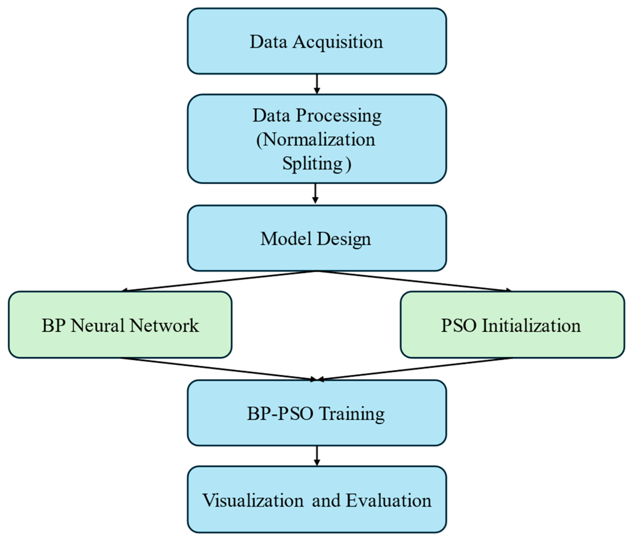
Figure 1. Framework of proposed wind resource assessment method.
Sustainability 17 10127 g001
Figure 2. Location of four sites including LHT, XCS, ZFD, and SSN. Each dot represents the geographical location of the site, where the red dot represents XCS, yellow one represents LHT, green represents ZFD and blue represents SSN.
Sustainability 17 10127 g002
Figure 3. Long-term wind speed frequency distributions in LHT, XCS, ZFD, and SSN. (a) LHT—distributions show moderate and stable wind speeds with narrow interannual variability. (b) XCS—wind-speed patterns remain consistent across years, indicating steady coastal conditions. (c) ZFD—distributions are broader with stronger seasonal fluctuations, reflecting more complex local terrain and higher turbulence. (d) SSN — wind-speed frequencies are concentrated within a higher range, demonstrating stronger and more persistent winds in the southeastern coastal region. The color gradient follows the colormap, where darker blue tones denote lower frequencies and yellow tones denote higher frequencies. μ and σ denote the mean and standard deviation of the fitted normal distribution.
Sustainability 17 10127 g003
Figure 4. Training and testing dataset of two splitting methods.
Sustainability 17 10127 g004
Figure 5. Predicted and actual hourly wind speeds and the corresponding error distribution at LHT for the multi-year BP-PSO model (2022). The time-series plot (left) shows agreement between observations and forecasts, while the histogram (right) demonstrates a near-error distribution centered close to zero.
Sustainability 17 10127 g005
Figure 6. Predicted and actual hourly wind speeds and the corresponding error distribution at XCS for the multi-year BP-PSO model (2022). The time-series plot (left) shows agreement between observations and forecasts, while the histogram (right) demonstrates error distribution centered close to zero.
Sustainability 17 10127 g006
Figure 7. Predicted and actual hourly wind speeds and the corresponding error distribution at ZFD for the multi-year BP-PSO model (2022). The time-series plot (left) shows agreement between observations and forecasts, while the histogram (right) demonstrates a near-error distribution centered close to zero.
Sustainability 17 10127 g007
Figure 8. Predicted and actual hourly wind speeds and the corresponding error distribution at SSN for the multi-year BP-PSO model (2022). The time-series plot (left) shows agreement between observations and forecasts, while the histogram (right) demonstrates an error distribution centered close to zero.
Sustainability 17 10127 g008
Figure 9. Predicted and actual hourly wind speeds for four seasons at LHT (2022) using the BP-PSO model (W = 24 h, H = 1 h).
Sustainability 17 10127 g009
Figure 10. Seasonal prediction-error distributions at site LHT using the BP-PSO model.
Sustainability 17 10127 g010
Figure 11. Predicted and actual hourly wind speeds for four seasons at XCS (2022) using the BP-PSO model (W = 24 h, H = 1 h).
Sustainability 17 10127 g011
Figure 12. Seasonal prediction-error distributions at site XCS using the BP-PSO model.
Sustainability 17 10127 g012
Figure 13. Predicted and actual hourly wind speeds for four seasons at ZFD (2022) using the BP-PSO model (W = 24 h, H = 1 h).
Sustainability 17 10127 g013
Figure 14. Seasonal prediction-error distributions at site ZFD using the BP-PSO model.
Sustainability 17 10127 g014
Figure 15. Predicted and actual hourly wind speeds for four seasons at SSN (2022) using the BP-PSO model (W = 24 h, H = 1 h).
Sustainability 17 10127 g015
Figure 16. Seasonal prediction-error distributions at site SSN using the BP-PSO model.
Sustainability 17 10127 g016
Figure 17. The annual predicted wind speeds over 2022 with shaded bands representing the 90% prediction interval derived by MC-Dropout (top-left: LHT, top-right: XCS; bottom-left: ZFD; bottom-right: SSN).
Sustainability 17 10127 g017
Figure 18. RMSE (left), R2 (mid), and MAE (right) of BP-PSO wind speed forecasts at four sites under different training methods.
Sustainability 17 10127 g018
Figure 19. Correlation matrices of observed (all-time) and BP-PSO-predicted wind speeds for four stations. (a) is the all-time correlation, (b) is correlation calculated by spring data, (c) is correlation calculated by summer data, (d) is correlation calculated by autumn data and (e) is correlation calculated by winter data.
Sustainability 17 10127 g019
Table 1. BP settings.
Key ParametersValue
number of neural network layers2
number of neurons in the first layer150
number of neurons in the second layer50
learning rate0.000032
batch size32
dropout ratio0.1–0.3
Table 2. PSO method settings.
Key ParametersValue
ω 0.5
c 1 1.8
c 2 2.0
Table 3. Coordination of four sites.
Longitude (°E)Latitude (°N)
LHT121.738.9
XCS122.739.2
ZFD121.437.6
SSN122.830.8
Table 4. Index in four sites.
Training DatasetsIndexLHTXCSZFDSSN
Multi-yearRMSE1.2701.0911.5411.285
R20.7000.7460.6310.854
MAE0.9320.7921.1010.942
NRMSE0.3200.3270.3770.215
Skill vs. Persistence0.0450.0440.0580.035
Skill vs. Arima0.5320.5240.4410.626
RMSE_CI1.219–1.3121.051–1.1301.462–1.6211.213–1.367
SpringRMSE1.3951.1861.5851.438
R20.6320.6250.5730.798
MAE1.0360.8651.1861.066
NRMSE0.3300.3580.3730.262
Skill vs. Persistence0.0540.0520.063−0.002
Skill vs. Arima0.4010.3950.3580.553
RMSE_CI1.303–1.3631.095–1.2621.485–1.6781.339–1.537
SummerRMSE1.1640.9811.3991.237
R20.5940.6040.5550.735
MAE0.8770.7081.0670.952
NRMSE0.3600.3780.3820.259
Skill vs. Persistence0.0630.0540.0680.029
Skill vs. Arima0.3630.3770.3340.502
RMSE_CI1.093–1.2400.899–1.0661.299–1.4991.165–1.291
AutumnRMSE1.2071.0831.6411.343
R20.7710.8120.6970.869
MAE0.8830.7631.0620.932
NRMSE0.3000.3110.4020.205
Skill vs. Persistence0.0220.0270.0260.044
Skill vs. Arima0.5880.5770.4580.646
RMSE_CI1.115–1.2930.995–1.1761.420–1.8771.128–1.580
WinterRMSE1.3181.1281.5431.172
R20.6970.7640.6240.884
MAE0.9940.8611.1340.883
NRMSE0.2990.2830.3540.165
Skill vs. Persistence0.0180.0210.0550.017
Skill vs. Arima0.5880.5150.3930.662
RMSE_CI1.229–1.3871.062–1.1861.431–1.6471.116–1.248
Disclaimer/Publisher’s Note: The statements, opinions and data contained in all publications are solely those of the individual author(s) and contributor(s) and not of MDPI and/or the editor(s). MDPI and/or the editor(s) disclaim responsibility for any injury to people or property resulting from any ideas, methods, instructions or products referred to in the content.