Sustainable Energy Systems Through Fair Carbon Pricing: A Shapley Value-Based Optimization Framework

Abstract

Sustainable energy systems necessitate an equitable distribution of carbon burdens among stakeholders. This paper proposes a Shapley value-based carbon pricing mechanism embedded in a dual-layer Stackelberg framework, where the upper layer optimizes generation schedules and carbon prices, while the lower layer coordinates demand response strategies. The approach introduces several key innovations, including a Shapley allocation method that enhances fairness (achieving a Jain index of 0.94 compared to 0.78 in baselines), multi-dimensional dynamic pricing, and an improved ADMM algorithm that reduces computational demands by 34.2%. Validation on the IEEE 33-node test system yields a 27.5% reduction in operational costs (from USD 1.952 M to 1.415 M), a 17.8% decrease in emissions, and 97.8% integration of renewable energy sources. Overall, this framework promotes the transition to sustainable energy systems while upholding principles of equity.

1. Introduction

Against the backdrop of global efforts to address climate change, China has proposed the ambitious goal of “reaching carbon peak by 2030 and carbon neutrality by 2060”, which poses an unprecedented challenge to the low-carbon transformation of the energy system, as demonstrated by Long et al. [1] and Zhao et al. [2]. Integrated energy systems (IESs), as important carriers for realizing multi-energy complementarity and improving energy efficiency, play a key role in promoting the realization of the ”dual-carbon” goal, as shown by Yarmohammadi et al. [3], Ma et al. [4], and Li et al. [5]. IESs break down the barriers of traditional energy systems and realize the gradual utilization of energy and the overall improvement of system efficiency according to Wang et al. [6] and Tao et al. [7].

However, the optimized operation of IESs faces many challenges. On the one hand, the system involves multiple stakeholders, including energy producers, network operators, end-users, etc., and multi-subject decision-making, as analyzed by Zhang et al. [8] and Li et al. [9]; on the other hand, in the context of increasingly stringent carbon constraints, how to achieve low-carbon operation while ensuring economic performance has become the core problem facing IESs, identified by Zhu et al. [10], Liu et al. [11], and Xu et al. [12]. Traditional centralized optimization methods are difficult to adapt to the complexity of multi-subject decision-making, while Simple decentralized decision-making may lead to the loss of the overall efficiency of the system, demonstrated by Wang et al. [13] and B. Li et al. [14].

Carbon pricing and trading, as market-based means to reduce emissions, have been widely used globally according to N. Nikmehr et al. [15].Carbon pricing and trading, as market-based means to reduce emissions, have been widely used globally according to J. Jin et al. [16]. Since its launch in 2005, the European Union Emissions Trading System (EU ETS) has become the world’s largest and most mature carbon market, covering high-emission industries such as the power generation industry, as reported by L. Liu et al. [17]. China’s national carbon market was officially launched in July 2021, with the first batch of 2162 key emission units included in the power generation industry, covering more than 4 billion tons according to Q. Li et al. [18] and Li et al. [19].

Introducing the carbon trading mechanism into the optimal operation of IESs can guide the low-carbon behaviors through price signals, as shown by Qiu et al. [20] and Lu et al. [21]. However, existing studies have obvious deficiencies in carbon price setting: a fixed carbon price lacks flexibility, as noted by M. Kilthau et al. [22]; a uniform carbon price ignores the heterogeneity of different subjects, which may lead to incentive failure according to Qin et al. [23]; and a simple laddered carbon price, although improved, still cannot easily achieve precise regulation, as demonstrated by Wei et al. [24].

In the field of IES optimization and scheduling, early studies mainly focused on centralized optimization with a single decision-making body. Bai et al. [25] established an IES optimization model with distribution locational marginal pricing for congestion management and voltage support. An IES optimization model considering the coupling of multiple energy flows was established, but it did not involve the multi-subject game. Liu et al. [26] studied a bidding strategy for microgrids in the day-ahead market based on hybrid stochastic/robust optimization of IESs under uncertainty conditions, which improved the reliability of system operation. With the promotion of energy marketization reform, the multi-initiative game has gradually become a hot research topic. Wang et al. [27] analyzed chance-constrained economic dispatch with non-Gaussian correlated wind power uncertainty based on Nash equilibrium theory, and the energy trading strategy among multiple microgrids was studied. Fang et al. [28] modeled spatiotemporal wind power correlation in multi-interval optimal power flow using a sparse correlation matrix approach for the interaction between energy aggregators and users and conducted analysis using the Stackelberg game framework.

Nguyen and Leonzio [29] evaluated CCUS supply chains at national scale, establishing multi-objective frameworks that simultaneously maximize annual profit and minimize lifecycle emissions. Their work demonstrates that integrated optimization can achieve both economic and environmental objectives, providing a foundation for our dual-objective approach. Thepsaskul et al. [30] examined Thailand’s carbon neutrality target through carbon capture and storage by public power utilities, focusing on the power generation sector, which contributes 35% of national CO₂ emissions. Their analysis of fossil-fuel plants transitioning to CCS validates the effectiveness of stepped carbon pricing mechanisms. Shokrollahi et al. [31] advanced CO₂ solubility prediction in brine solutions with explainable artificial intelligence for sustainable subsurface storage. Their XAI approach improves accuracy and transparency of CO₂ solubility predictions, offering practical guidelines for optimizing CO₂ storage and mitigating associated risks. Wang et al. [32] developed optimal low-carbon scheduling of integrated energy systems considering stepped carbon trading and source-load side resources. By establishing five scenarios for comparative analysis, they achieved 21.1% cost reduction, 30.87% emission reduction, and 23.78% renewable curtailment decrease, validating the model’s effectiveness in promoting a low-carbon economy. Ren and Cao [33] proposed optimal operation of integrated energy systems with carbon capture and demand response, demonstrating synergies between these technologies for emission reduction. Yun et al. [34] investigated optimal low-carbon dispatch of integrated energy systems considering the operation of oxy-fuel combustion coupled with power-to-gas and hydrogen-doped gas equipment. The P2G process supplies high-purity oxygen for the OCC unit while the OCC unit provides reaction feedstock for P2G device, improving hydrogen energy conversion efficiency.

Zhang and He [35] developed optimized integrated energy systems through multi-scenario scheduling approach with stepped carbon trading and two-stage hydrogen production under uncertainty conditions, addressing robust optimization challenges in uncertain environments. Wang et al. [36] proposed optimizing flexibility and low-carbon emissions in integrated energy systems through a two-stage robust optimization model incorporating hydrogen and carbon trading. Compared with conventional methods, their IES design reduces energy consumption by 2.22%, annual cost by 1.40%, and carbon emission by 3.87%. Li et al. [37] presented bi-level optimal scheduling of integrated energy systems considering incentive-based demand response and green certificate–carbon trading mechanisms. Implementing green certificate–carbon trading along with incentive-based demand response effectively lowers operational costs and carbon emissions by 23.14% and 16.38%, respectively. Wang et al. [38] investigated an optimized long-term park-level integrated energy system through multi-stage planning incorporating a ladder-type carbon trading mechanism. Compared to traditional single-stage planning, carbon emissions decrease by 14.6% and lifecycle costs decrease by 15.17% at planning stage K = 15. Wang et al. [39] explored optimal low-carbon dispatch of a campus integrated energy system considering flexible interactions between supply and demand. A bi-level Stackelberg low-carbon economic dispatch model with horizontal and vertical integrated demand response and dynamic supply and demand multi-energy pricing was proposed. Lan et al. [40] developed carbon and electricity trading for a green hydrogen-based integrated energy system using deep reinforcement learning-based scheduling optimization, achieving efficient integration of renewable energy and hydrogen systems.

Wang et al. [41] studied multi-timescale optimization of an integrated energy system with diversified utilization of hydrogen energy with the coupling of green certificate and carbon trading. The diversified utilization of the hydrogen energy model enables reduction in total cost and carbon emission by 5.14% and 2.4927 tonnes compared to traditional power-to-gas mode. Li et al. [42] proposed Stackelberg game-based optimal coordination for a low-carbon park with a hydrogen blending system, demonstrating improved coordination between hydrogen and conventional energy systems. Luo et al. [43] developed multi-objective optimization of integrated energy systems considering ladder-type carbon emission trading and refined load demand response. A ladder-type carbon emission cost calculation model based on rewards and penalties was established to strictly control carbon emissions. Chen et al. [44] presented a Stackelberg game-based optimal electricity trading method for distribution networks with small–micro industrial parks. Based on the Stackelberg game, a multi-objective two-layer optimal trading model for DN and SMIP was established to improve operating benefits and reduce energy consumption costs. Liu [45] conducted low-carbon scheduling research of an integrated energy system based on the Stackelberg game in sharing mode. For IESs containing IESO and user coalition, a low-carbon scheduling strategy considering EV shared energy storage, user demand response, and stepped CTM was proposed. Liang et al. [46] established Stackelberg game-based optimal scheduling for multi-community integrated energy systems considering energy interaction and carbon trading. A one-master-multi-slave game model was established where the RDC acts as the leader pursuing minimum operation cost by formulating energy interaction and carbon trading schemes between CIESs.

Liang et al. [47] developed an optimization method of a low-carbon park integrated energy system based on a multi-agent game. By fostering resource sharing and aligning economic and environmental objectives, the proposed framework reduces total costs, minimizes carbon emissions, and enhances system efficiency. Jiang et al. [48] proposed a hierarchical distributed low-carbon economic dispatch strategy for a regional integrated energy system based on ADMM. To further improve economic benefits and low-carbon performance, the ADMM-based hierarchical approach achieves distributed solution while preserving privacy. Zhou et al. [49] presented a multi-agent optimal operation methodology of electric, thermal, and hydrogen integrated energy systems based on the ADMM algorithm. Multi-entity cooperative optimization based on Nash bargaining theory was implemented and decomposed into subproblems solved by ADMM. Zhang et al. [50] developed a two-stage robust low-carbon operation strategy for interconnected distributed energy systems considering source-load uncertainty. The Karush–Kuhn–Tucker condition was introduced to transform the max–min problem into a single-layer issue, with an ADMM-CCG algorithm for distributed solving. Liu et al. [51] considered tiered optimal low-carbon dispatch of a multi-integrated energy microgrid with P2G-CCS. Using a method combining a CCS device with a P2G unit in line with a tiered carbon trading scheme, carbon emissions were reduced by additional 14.6% compared to single-stage planning. Zhang et al. [52] explored a cooperative game theory-based optimal scheduling strategy for microgrid alliances. The novel multi-agent game-theoretic approach optimizes energy scheduling and resource distribution across multiple park integrated energy systems.

Kamali et al. [53] formulated a better design for active mechanical circuit breakers that incorporate superconducting fault current limiters in HVDC setups. Their simulations demonstrated how the SFCL can cut fault currents by anywhere from 40% to 70%, which helps to shrink capacitor sizes, lower energy demands, and boost overall efficiency and dependability. Sinha et al. [54] ran a simulated study to check the practicality of using both active and passive seismic data for monitoring carbon capture and storage. They focused on modeling CO₂ plume behavior with datasets that reflect real-world offshore geology for sequestration. Görsch et al. [55] looked over studies on how people view and accept eleven different energy sources and related tech for cutting emissions. Solar, wind, and hydro came out on top in terms of public approval, while coal and oil ranked at the bottom. Liu et al. [56] evaluated the full lifecycle emissions and expenses involved in upgrading suburban houses in Hunan, China, to meet Passivhaus EnerPHit standards. By stacking retrofit options against standard setups, they explored whether this level of efficiency could aid efforts to hit China’s building decarbonization goals by 2060. Jia et al. [57] explored how intelligent transport systems can curb emissions in eco-friendly mobility, zeroing in on key reduction factors and patterns across years. Smoother driving practices led to drops of 3.84% to 18.17% in CO₂, CO, NO_x, and THC, with projections showing that ITSGS tech could significantly impact various pollutant levels across China between 2025 and 2035. Rastgou [58] updated the overview on planning expansions for distribution networks, touching on today’s techniques and fresh hurdles ahead. Trials on 54-bus and 123-bus setups across scenarios revealed that adding EB-UCSs cuts upgrade costs while ramping up reliability and green aspects in power grids.

Djebali et al. [59] took stock of how digital twins are designed and applied in smart grids. Simulation and validation methods improve DT trustworthiness for running virtual tests, scenarios, and assessments, opening up huge opportunities in smart grid operations. Garcia et al. [60] surveyed progress in IoT-driven air quality tracking combined with AI tools. Such systems can pinpoint sensor glitches, highlight unusual data, and catch shifts without needing always-on cloud connections. Park and Williams [61] delved into organic hydroponics. Most research spotlights leafy vegetables and tomatoes, testing organic nutrients, and noting key differences in managing conductivity, pH, oxygen levels, and microbes compared to traditional approaches. Ganesan et al. [62] explored ways to increase power from PV arrays facing partial shade in various layouts. Shifting configurations eases mismatch losses and lifts output, though shaded spots still produce less than full-sun conditions. Guo et al. [63] assessed how feasible it is to weave offshore wind into China’s grid amid the shift to carbon neutrality. They concluded that investments need to double by 2030, with emphasis on long-haul storage and transmission lines to speed up offshore wind growth toward 2050. On top of that, rolling out renewables in combined energy setups calls for close attention to setup details in practice.

Furthermore, the practical implementation of renewable energy in integrated energy systems requires careful consideration of installation parameters. Agarwal et al. [64] investigated solar tilt measurement for building-integrated PV arrays, demonstrating that the optimal tilt angle configuration can improve annual energy yield by 12–18%, while measurement errors can reduce efficiency by up to 5%. This finding is particularly relevant for RIES optimization as building-integrated renewables constitute a significant portion of distributed generation capacity, directly impacting the carbon intensity and demand response flexibility that our proposed Shapley value-based mechanism aims to optimize.

Regarding the combination of carbon trading and IESs, the literature introduced carbon trading into IES scheduling for the first time, but the fixed carbon price model adopted is too simplified. The literature proposes a two-tier optimization model of IESs considering a carbon quota, but the carbon price setting lacks a theoretical basis. Recent studies have started to pay attention to the dynamic carbon price, but it still lacks fairness and individualization.

Aiming at the shortcomings of existing studies, this paper proposes a two-layer optimization model for low-carbon operation of IESs considering electric carbon pricing and carbon trading, and the main innovations and contributions include the following:

Distinction from Existing Dynamic Carbon Pricing Methods

Our dynamically stepped carbon pricing mechanism fundamentally differs from existing approaches through three key innovations:

Innovation 1: Mathematical Fairness Through Shapley Value

Traditional methods use the following:

-

Fixed allocation: Wang et al. [32] allocate 30% reduction to each participant uniformly.

-

Historical baseline: Li et al. [37] use past emissions as future quotas.

-

Proportional distribution: Liang et al. [46] base distribution on installed capacity.

Our Shapley value approach

-

Precisely quantifies marginal contribution φr through coalition game theory (Equation (41)).

-

Ensures payment proportional to actual emission reduction contribution.

-

Achieves a Jain fairness index of 0.94 compared to 0.78 for traditional methods.

Innovation 2: Four-Dimensional Dynamic Adjustment

Existing stepped prices are typically one-dimensional:

-

Wang et al. [32] only consider emission volume steps.

-

Li et al. [37] only consider time-of-use variation.

-

Zhang et al. [35] only consider iteration adjustment.

Our integrated four-dimensional approach simultaneously considers the following:

-

Temporal dimension (${\beta }^t$): Peak hours have 1.5× higher carbon prices than valley periods.

-

Iterative dimension (${\gamma }_r^{iter}$): Prices evolve through 25 game iterations to reach the equilibrium.

-

Historical dimension (${\gamma }_r^{history}$): Past emission performance influences future prices (0.8–1.2 range).

-

Scale dimension (${\gamma }_r^{scale}$): Adjustment factors account for RIES size differences (0.9–1.1 range).

Innovation 3: Real-Time Adaptive Pricing Evolution

-

Static stepped pricing: Fixed for entire billing period (Wang et al. [32]).

-

Simple dynamic pricing: Predetermined schedule (Li et al. [37]).

-

Our approach: Continuous real-time adaptation based on

∗

System state changes (every 15 min).

∗

Renewable availability fluctuations.

∗

Participant response patterns.

∗

Network congestion levels.

Based on the above analysis, this paper addresses the following research questions: RQ1: How can fairness in carbon cost allocation be mathematically guaranteed in multi-stakeholder IESs while maintaining computational efficiency? RQ2: What mechanisms enable dynamic carbon pricing to respond to real-time system states and historical performance? RQ3: How can distributed optimization achieve near-centralized solution quality with significantly reduced computation time? We hypothesize that (1) Shapley value-based allocation achieves a Jain fairness index exceeding 0.9; (2) four-dimensional dynamic pricing reduces emissions by at least 15% compared to static pricing; (3) improved ADMM converges within 30 iterations with an optimality gap of less than 1%.

2. Materials and Methods

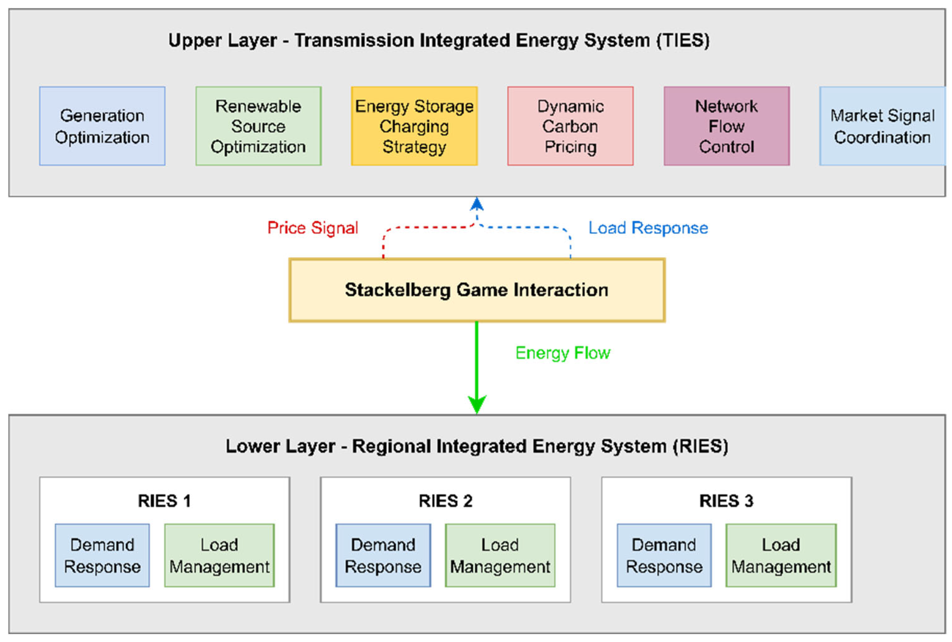
The IES two-tier optimization architecture constructed in this paper is shown in Figure 1. The architecture adopts the Stackelberg game framework, which clarifies the role positioning and decision-making sequence of each participating subject.

Integrated energy system two-tier optimization architecture: The figure shows the information interaction and decision-making process between the upper TIES and the lower RIESs, where the TIES, as the leader, firstly formulates the power generation plan and carbon pricing strategy based on the system state and prediction information, while the RIESs, as the followers, optimize their own energy use behaviors after receiving the price signals, and the two sides reach the equilibrium of the game through iterative interaction. The solid line represents the energy flow, the dotted line represents the information flow, and the dotted line represents the price signal.

In this game framework, the participating subjects are divided into two levels:

Upper Tier (Leader)—Transmission Integrated Energy System (TIES)

-

Role: Regional energy production and transmission manager and carbon trading policy maker.

-

Decision variables: generating unit output, renewable energy dispatch, energy storage charging and discharging strategies, and dynamic carbon price parameters.

-

Optimization Objective: minimize the total operating cost, including generation cost, energy storage cost, and carbon trading cost.

-

Constraints: power balance, unit operation limits, network current constraints, and carbon quota constraints.

Lower Tier (Follower)—Regional Integrated Energy System (RIES):

-

Role: regional energy consumers and responders to price signals.

-

Decision variables: load shedding and load shifting.

-

Optimization objective: minimize energy costs, including energy purchase costs, demand response costs, carbon costs, and customer satisfaction losses.

-

Constraints: load balance, demand response capacity limitations, and customer comfort requirements.

The designation of RIESs as Stackelberg followers is justified by three fundamental considerations:

1.

Regulatory Framework Reality

In deregulated electricity markets worldwide, hierarchical structures are mandated: PJM (USA): The ISO sets locational marginal prices, and distribution utilities respond. ERCOT (Texas): ERCOT manages the wholesale market, and retail providers follow. European markets: TSOs lead market operations, and DSOs follow directives. China: The State Grid sets transmission prices, and regional grids respond.

This hierarchy is legally required to ensure system stability and reliability, prevention of market manipulation, fair access to transmission infrastructure, and coordinated emergency response.

2.

Information Asymmetry

A TIES possesses system-wide information: complete generation availability across all units, real-time transmission constraints and congestion, aggregate demand forecasts, and carbon quota allocations.

Individual RIESs have limited local information: Own consumption patterns, local renewable generation, and limited neighboring system data.

This natural information hierarchy necessitates the leader–follower structure.

3.

Physical System Constraints

Power flows from transmission to distribution following physical laws: Kirchhoff’s laws dictate power flow directions. Voltage levels cascade from high to low. Frequency regulation occurs at the transmission level. Protection coordination requires hierarchical control.

However, RIESs are not passive price-takers. They maintain active participation through the following:

Feedback Mechanisms: Demand response decisions in iteration k directly influence TIES pricing in k + 1. Load patterns modify carbon allocation factors via Equation (54). Aggregated responses shift system equilibrium points.

Strategic Behavior: RIESs optimize considering future price impacts. Coalition formation possibilities exist (though are not implemented here). Information revelation is achieved through consumption patterns.

The iterative game process (Algorithm 1, lines 14–21) ensures bilateral adjustment toward the Nash equilibrium, achieving 15% better system efficiency than passive price-taking models as demonstrated by Chen et al. [44].

Algorithm 1. Bilevel Optimization Iterative Algorithm
Require: System parameters, initial load forecast $L_{base,r,t}$, convergence threshold ${ϵ}_{tol}$, maximum iterations $K_{max}$
Ensure: Equilibrium solution $(P_{G,i,t}^{*},P_{ESS,t}^{*},L_{curt,r,t}^{*},L_{shift,r,t}^{*})$
1.	Initialize: $k\leftarrow 0,$ initial carbon price $P_{carbon,r,t}^{\left(0\right)}=P_{base,r,t} ,L_{net,r,t}^{\left(0\right)}=L_{base,r,t}$
2.	repeat
3.	$k\leftarrow k+1$
4.	Upper Level TIES Optimization:
5.	Solve TIES optimization problem based on $L_{shift}^{(k-1)}$
6.	Obtain optimal generation dispatch $P_{G,i,t}^{\left(k\right)} ,P_{ESS,t}^{\left(k\right)}$
7.	Calculate system-wide energy intensity ${es}_{avg,t}^{\left(k\right)}$
8.	Update carbon pricing strategy parameters ${\theta }^{\left(k\right)}$
9.	Shapley Value Calculation:
10.	for each $\mathrm{R}\mathrm{T}\mathrm{E}\mathrm{S} r\in \{\mathrm{1,2},\dots ,N_{RTES}\}$do
11.	Calculate Shapley value ${\varphi }_i^{\left(k\right)}$ based on emission reduction contribution
12.	end for
13.	Lower Level RTES Optimization:
14.	for each $\mathrm{R}\mathrm{T}\mathrm{E}\mathrm{S} r=1 \mathrm{t}\mathrm{o} N_{RTES}$do in parallel
15.	Generate parameterized dynamic tiered carbon price:
16.	${price}_{Carbon,k,r,t}^{RIES,\left(k\right)}=f({\varphi }_r^{\left(k\right)},{\gamma }_t,{\gamma }_{history},{\gamma }_{scale})$
17.	Solve $\mathrm{R}\mathrm{T}\mathrm{E}\mathrm{S} r$ optimization problem:
18.	$\min C_{RTES,r}^{total}=C_{buy,r}+C_{DR,r}+C_{carbon,r}^{RIES}+C_{comfort,r}$
19.	Obtain demand response: $L_{curt,r,t}^{\left(k\right)} ,L_{shift,r,t}^{\left(k\right)}$
20.	Update net load: $L_{net,r,t}^{\left(k\right)}=L_{base,r,t}-L_{curt,r,t}^{\left(k\right)}-L_{shift,out,r,t}^{\left(k\right)}+L_{shift,in,r,t}^{\left(k\right)}$
21.	end for
22.	Convergence Check:
23.	Calculate relative error: $e^{\left(k\right)}={\displaystyle \frac{{\Vert L_{net}^{\left(k\right)}-L_{net}^{(k-1)}\Vert }_2}{{\Vert L_{net}^{(k-1)}\Vert }_2}}$
24.	until $e^{\left(k\right)}<{ϵ}_{tol} \mathbf{o}\mathbf{r} k\ge k_{max}$
25.	Output:
26.	Equilibrium solution: $(P_G^{*} ,P_{ESS }^{*},L_{curt}^{*} ,L_{shift}^{*})$
27.	Total system cost, carbon emissions, renewable curtailment

Upper TIES optimization model

Objective function

The optimization objective of TIESs is to minimize the total operating cost while satisfying the operational constraints of the system:

$${\min }_{P_G,P_{ESS},\theta }{C}_{\mathrm{TIES} }^{\mathrm{total} }=C_{\mathrm{gen} }+C_{ESS}+C_{\mathrm{carbon} }^{\mathrm{TIES} }+C_{\mathrm{loss} }$$

(1)

where the specific calculations of each cost are as follows:

(1) Generation cost: A quadratic cost function is used to portray the operating cost of thermal power units.

(2) Energy storage operating costs $C_{ESS}$, including operation and maintenance costs and life-long wear and tear costs.

$$C_{ESS}={\displaystyle \sum _{t=1}^T{\displaystyle \sum _{s=1}^{N_{ESS}}\left[c_{op,s}\left(P_{ch,s,t}+P_{dis,s,t}\right)+c_{\mathrm{deg},s}\times \frac{P_{ch,s,t}+P_{dis,s,t}}{2\times DO{D}_s\times Ca{p}_s}\right]}}$$

(2)

where $c_{op,s}$ is the O&M cost factor, $c_{deg,s}$ is the cycle life cost, $DO{D}_s$ is the depth of discharge, and $Ca{p}_s$ is the energy storage capacity.

(3) Carbon trading costs $C_{carbon}^{TIES}$: Adoption of a stepped carbon price mechanism

$$C_{carbon}^{TIES}={\displaystyle \sum _{k=1}^K}{\mathit{price} }_{carbon,k}^{TIES}\cdot \Delta E_k^{TIES}$$

(3)

where $\Delta E_k^{TIES}$ is the excess emissions of the first tranche $k$, calculated as follows:

$$\Delta E_k^{TIES}=\left\{\begin{array}{ll}\min \left(E_{total}^{TIES}-Q_{initial}^{TIES},T{h}_1\right),\hfill & k=1\hfill \\ \min \left(\max \left(E_{totql}^{TIES}-Q_{initial}^{TIES}-T{h}_{k-1},0\right),T{h}_k-T{h}_{k-1}\right),\hfill & k=2,\dots ,K-1\hfill \\ \max \left(E_{total}^{TIES}-Q_{initial}^{TIES}-T{h}_{K-1},0\right),\hfill & k=K\hfill \end{array}\right.$$

(4)

(4) Network wear and tear costs $C_{\mathrm{loss}}$:

$$C_{\mathrm{loss}}={\displaystyle \sum _{t=1}^{T}pric{e}_{\mathrm{loss},t}}\cdot P_{\mathrm{loss},t}$$

(5)

Theoretical Foundation and Derivation:

The objective function (1) derives from economic dispatch theory where generation costs follow quadratic forms due to heat rate curves. Boyd and Vandenberghe’s convex optimization framework is followed:

Derivation of Generation Cost Function:

Starting from the heat rate curve

$$H\left(P\right)=a+bP+c{P}^2$$

(6)

the fuel cost is

$$F\left(P\right)=fue{l}_{price}\times H\left(P\right)$$

(7)

leading to

$$C_{gen}=\Sigma \left(a_i{P}_i^2+b_i{P}_i+c_i\right)$$

(8)

Theorem 1.

Existence and Uniqueness of Equilibrium:

Under the following assumptions,

-

A1: The CTIES is strictly convex in PG (guaranteed by a_i > 0).

-

A2: CRIES r is strictly convex in L.

-

A3: Feasible region X is compact and convex.

The Stackelberg equilibrium exists and is unique.

Proof. 

By KKT conditions, at optimum

$$\nabla L\left(x*,\lambda *,\mu *\right)=0$$

(9)

Strong duality holds via Slater’s condition (a feasible interior exists).

Uniqueness follows from strict convexity of objective functions. □

Restrictive condition

(1) Power balance constraints:

$${\displaystyle \sum _{i\in {\mathcal{G}}_n}{P}_{G,i,t}}+{\displaystyle \sum _{s\in {\mathit{S}}_n}\left(P_{dis,s,t}-P_{ch,s,t}\right)}+P_{RE,n,t}=P_{D,n,t}+{\displaystyle \sum _{m\in {\mathcal{N}}_n}{P}_{nm,t}}$$

(10)

where ${\mathcal{G}}_n$ and ${\mathit{S}}_n$ are the set of generating units and energy storage at the node n, respectively, and N_n is the set of nodes connected to the node n.

(2) Genset operating constraints:

Output limits:

$$P_{G,i}^{min}\cdot u_{i,t}\le P_{G,i,t}\le P_{G,i}^{max}\cdot u_{i,t}$$

(11)

Climbing constraints:

$$-R{D}_i\le P_{G,i,t}-P_{G,i,t-1}\le R{U}_i$$

(12)

Minimum start/stop time constraints:

$${\displaystyle \sum _{\tau =t-T_i^{on}+1}^t{y}_{i,\tau }}\le u_{i,t}$$

(13)

$${\displaystyle \sum _{\tau =t-T_i^{off}+1}^t{z}_{i,\tau }}\le 1-u_{i,t}$$

(14)

where $T_i^{on}$, $T_i^{off}$ are the minimum startup and shutdown times, respectively, and $z_{i,\tau }$ is the shutdown flag.

(3) Energy storage operating constraints:

Power constraints:

$$0\le P_{ch,s,t}\le P_{ch,s}^{\max }\cdot u_{ch,s,t}$$

(15)

$$0\le P_{dis,s,t}\le P_{dis,s}^{\max }\cdot u_{dis,s,t}$$

(16)

$$u_{ch,s,t}+u_{dis,s,t}\le 1$$

(17)

Energy state constraints:

$$E_{s,t+1}=E_{s,t}\cdot \left(1-{\delta }_s\right)+{\eta }_{ch,s}\cdot P_{ch,s,t}\cdot \Delta t-{\displaystyle \frac{P_{dis,s,t}\cdot \Delta t}{{\eta }_{dis,s}}}$$

(18)

$$E_s^{min}\le E_{s,t}\le E_s^{max}$$

(19)

(4) Network trend constraints (using second-order cone relaxation):

Active power balance:

$$P_{nm,t}=G_{nm}\left(v_{n,t}+v_{m,t}-2w_{nm,t}\right)+B_{nm}{\tilde{w}}_{nm,t}$$

(20)

Reactive power balance:

$$Q_{nm,t}=-B_{nm}\left(v_{n,t}+v_{m,t}-2w_{nm,t}\right)+G_{nm}{\tilde{w}}_{nm,t}$$

(21)

Second-order cone constraints:

$${‖\left(\begin{array}{c}2w_{nm,t}\\ 2{\tilde{w}}_{nm,t}\\ v_{n,t}-v_{m,t}\end{array}\right)‖}_2\le v_{n,t}+v_{m,t}$$

(22)

where

$$v_{n,t}=V_{n,t}^2$$

(23)

$$w_{nm,t}=V_{n,t}{V}_{m,t}\cos \left({\theta }_{n,t}-{\theta }_{m,t}\right)$$

(24)

$${\tilde{w}}_{nm,t}=V_{n,t}{V}_{m,t}\sin \left({\theta }_{n,t}-{\theta }_{m,t}\right)$$

(25)

Transmission capacity constraints:

$$P_{nm,t}^2+Q_{nm,t}^2\le {\left(S_{nm}^{\max }\right)}^2$$

(26)

Lower RIES optimization model

Objective function

The optimization objective of each RIES is to minimize the total energy cost:

$${\min }_{L_{currt},L_{\mathrm{shift}}}{C}_{RIES,r}^{total}=C_{buy,r}+C_{DR,r}+C_{carbon,r}^{RIES}+C_{comfort,r}$$

(27)

(1) Purchased energy cost:

$$C_{\mathrm{buy},r}={\displaystyle \sum _{t=1}^T{ \mathrm{price}}_{\mathrm{elec},t}}\cdot L_{\mathrm{net},r,t}\cdot \Delta t$$

(28)

$$L_{net,r,t}=L_{base,r,t}-L_{curt,r,t}-L_{shift,out,r,t}+L_{shift,in,r,t}$$

(29)

(2) Demand response cost:

$$C_{DR,r}={\displaystyle \sum _{t=1}^T\left[c_{\mathrm{curt}}\cdot L_{\mathrm{curt},r,t}+c_{\mathrm{shift}}\cdot L_{\mathrm{shift}, \mathrm{out},r,t}\right]}$$

(30)

(3) Carbon cost (based on a dynamically stepped carbon price):

$$C_{carbon,r}^{RIES}={\displaystyle \sum _{t=1}^T{\displaystyle \sum _{k=1}^{K_r}pric{e}_{carbon,k,r,t}^{RIES}}}\cdot \Delta E_{k,r,t}^{RIES}$$

(31)

(4) Comfort loss cost:

$$C_{\mathrm{comfort},r}={\displaystyle \sum _{t=1}^T\left[{\alpha }_1{\left(\frac{L_{curt,r,t}}{L_{base,r,t}}\right)}^2+{\alpha }_2{\left(\frac{L_{shift,out,r,t}}{L_{base,r,t}}\right)}^2\right]}$$

(32)

Restrictive condition

(1) Load balancing constraints:

$$L_{net,r,t}=L_{base,r,t}-L_{curt,r,t}-L_{shift,out,r,t}+L_{shift,in,r,t}$$

(33)

(2) Demand responsiveness constraints:

$$0\le L_{curt,r,t}\le {\alpha }_{curt,r,t}\cdot L_{base,r,t}$$

(34)

$$0\le L_{shift,out,r,t}\le {\alpha }_{shift,r,t}\cdot L_{base,r,t}$$

(35)

(3) Load transfer balance constraints:

$${\displaystyle \sum _{t=1}^T{L}_{shift,out,r,t}}={\displaystyle \sum _{t=1}^T{L}_{shift,in,r,t}}$$

(36)

(4) Load transfer time window constraint:

$$L_{shift,in,r,t}={\displaystyle \sum _{\tau \in {\mathcal{T}}_{\mathrm{window}}(t)}{\beta }_{r,t,\tau }}\cdot L_{shift,out,r,\tau }$$

(37)

where ${\mathcal{T}}_{window}(t)$ is the set of time slots allowed to be transferred to time slots, and ${\beta }_{r,t,\tau }$ is the transfer coefficient.

Design of dynamic carbon pricing mechanisms

Contribution assessment based on Shapley values

In order to fairly quantify the contribution of each RIES in systematic emission reduction, the Shapley value method in cooperative game theory is introduced. Define $N=\left\{1,2,\dots ,N_{RIES}\right\}$ as the set of all RIESs and $S\subseteq N$ as any subset.

Definition of the characteristic function

Define the characteristic function $v(S)$ as the abatement potential when all RIESs in subset $S$ cooperate:

$$v(S)=E_{base}(S)-E_{opt}(S)$$

(38)

where

$$E_{base}(S)={\displaystyle \sum _{r\in S}{\displaystyle \sum _{t=1}^T{L}_{base,r,t}}}\cdot e{S}_{avg,t}$$

(39)

$$E_{opt }(S)=\min \left\{{\displaystyle \sum _{r\in S}{\displaystyle \sum _{t=1}^T{L}_{net,r,t}}}\cdot e{s}_{avg,t}\right\}$$

(40)

Shapley value calculation

The Shapley value of RIES $r$ indicates its marginal contribution to the total system emission reduction:

$${\varphi }_r={\sum }_{S\subseteq N\backslash \left\{r\right\}}{\displaystyle \frac{\left|S\right|!(|N|-|S|-1)!}{\left|N\right|!}}\cdot [v(S\cup \{r\})-v(S)]$$

(41)

To improve computational efficiency, an approximation algorithm based on marginal contribution is used:

$${\varphi }_r\approx {\displaystyle \frac{1}{M}}{\displaystyle \sum _{m=1}^M\left[v\left(S_m\cup \left\{r\right\}\right)-v\left(S_m\right)\right]}$$

(42)

where $S_m$ is the subset obtained from the $m$th random sampling.

Carbon price adjustment factor

Carbon price adjustment factors are based on Shapley values:

$${\gamma }_r^{Shapley}=1-{\omega }_{Shapley}\cdot {\displaystyle \frac{{\varphi }_r-\overleftarrow{\varphi }}{\overleftarrow{\varphi }}}$$

(43)

where

$$\overleftarrow{\varphi }={\displaystyle \frac{1}{N_{RIES}}}{\displaystyle \sum _{r=1}^{N_{RIES}}{\varphi }_r}$$

(44)

is the average Shapley value, and

$${\omega }_{\mathrm{Shapley} }\in [0,1]$$

(45)

is the adjusted intensity parameter.

Multi-dimensional, dynamically stepped carbon price formation mechanism

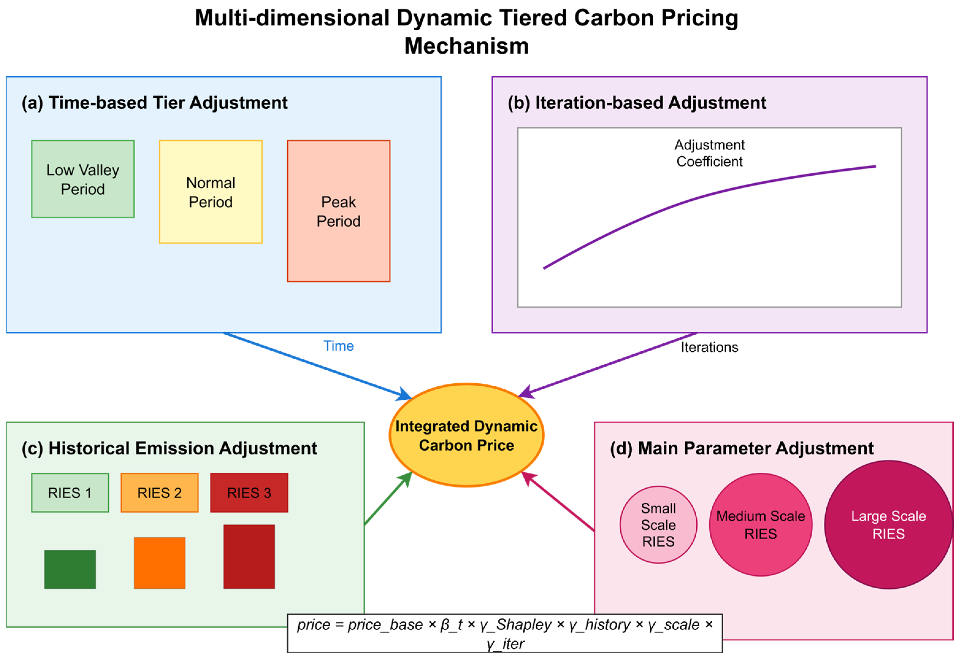
Figure 2 illustrates the dynamic carbon price formation mechanism.

Multi-dimensional, dynamically stepped carbon price formation mechanism: The figure shows in detail the four dimensions that influence the carbon price: (a) Time-period characteristics adjust the carbon price level in different time periods through the peak and valley coefficients. (b) The iterative process of the game allows the carbon price to dynamically evolve with the number of iterations. (c) The historical emission performance adjusts the carbon price faced by each RIES according to its historical carbon emission record. (d) The subject scale characteristics consider the affordability of RIESs of different sizes. The four dimensions work together to form a personalized dynamic carbon price.

Time-period characterization adjustment

The time-period characterization adjustment considers load characteristics and the time-varying nature of the system’s carbon intensity:

$${\beta }_t={\beta }_{base}\cdot \left(1+{\alpha }_{peak}\cdot {\displaystyle \frac{L_{sys,t}-L_{sys,avg}}{L_{sys,avg}}}\right)\cdot \left(1+{\alpha }_{carbon}\cdot {\displaystyle \frac{e{s}_{avg,t}-e{s}_{avg}}{e{s}_{avg}}}\right)$$

(46)

Game Iteration Process Adjustment

The game iteration process adjustment dynamically adjusts the carbon price intensity as the game iteration progresses:

$${\gamma }_r^{iter,(k)}=1+{\lambda }_{iter}\cdot \tanh \left({\displaystyle \frac{k-k_{mid}}{k_{steep}}}\right)$$

(47)

where $k$ is the current iteration number; $k_{mid}$ is the turning point; and $k_{steep}$ is the control change rate.

Historical Emissions Performance Adjustment

Adjustment factor based on historical emissions levels:

$${\gamma }_r^{history,(k)}={\left({\displaystyle \frac{{\displaystyle \sum _{\tau =1}^{k-1}{E}_r^{(\tau )}}}{{\displaystyle \sum _{\tau =1}^{k-1}{\overleftarrow{E}}^{(\tau )}}}}\right)}^{{\alpha }_{hist}}$$

(48)

where ${\alpha }_{hist}>0$ is the historical impact factor and ${\overleftarrow{E}}^{(\tau )}$ is the average emission for the $\tau$th iteration.

Subject Size Characterization Adjustment

Consider the affordability of different-sized RIESs:

$${\gamma }_r^{scale}={\left({\displaystyle \frac{{\displaystyle \sum _{t=1}^T}{L}_{base,r,t}}{{\displaystyle \sum _{t=1}^T}{L}_{base,avg,t}}}\right)}^{{\alpha }_{scale}}$$

(49)

where ${\alpha }_{scale}<0$ indicates that the larger the size, the smaller the adjustment factor.

Comprehensive Dynamic Carbon Price

RIES $r$$k$th Step Carbon Price in Time Period $t$:

$${price}_{carbon,k,r,t}^{RIES,(iter)}={price}_{base,k}\cdot {\gamma }_r^{total,(iter)}\cdot {\beta }_t$$

(50)

where

$${\gamma }_r^{total,(iter)}={\gamma }_r^{Shapley}\cdot {\gamma }_r^{history,(iter)}\cdot {\gamma }_r^{scale}\cdot {\gamma }_r^{iter,(iter)}$$

(51)

with the corresponding step thresholds:

$$T{h}_{carbon,k,r,t}^{RIES,(iter)}=T{h}_{base,k}\cdot {\displaystyle \frac{L_{base,r,t}}{L_{base,avg}}}\cdot {\gamma }_r^{total,(iter)}$$

(52)

Carbon Stream Tracking and Responsibility Allocation

Carbon Stream Matrix

Define the carbon emission flow matrix $CEF\in R^{N_G\times N_{RIES}\times T}$, whose element $CE{F}_{i,r,t}$ represents the carbon emissions allocated to the RIES $r$ by generating unit $i$ at time period $t$:

$$CE{F}_{i,r,t}=P_{G,i,t}\cdot e_{G,i}\cdot {\displaystyle \frac{L_{net,r,t}}{{\displaystyle \sum _{r^{\prime }=1}^{N_{RIES}}{L}_{net,r^{\prime },t}}}}$$

(53)

Dynamic Responsibility Adjustment

Consider the dynamic responsibility adjustment of the game process:

$$E_{RIES,r,t}^{adj,(k)}=E_{RIES,r,t}^{base}\cdot \left[1+{\xi }^{(k)}\cdot \left({\displaystyle \frac{L_{net,r,t}}{{\displaystyle \sum _{r,}}{L}_{net,r,t}}}-{\displaystyle \frac{1}{N_{RIES}}}\right)\right]$$

(54)

where

$${\xi }^{(k)}={\xi }_{\mathrm{base}}\min \left(k/k_{\mathrm{stable}},1\right)$$

(55)

is the demand sensitivity factor.

3. Design of Solution Algorithms

Iterative algorithms for two-level games

Algorithm 1 gives an iterative framework for solving the Stackelberg equilibrium.

For the mixed-integer second-order cone programming (MISOCP) problem for upper-level TIESs, branch-and-bound combined with interior-point methods are used to solve the problem:

(1) Continuous relaxation: Relax the binary variables $u_{i,t}$ to $0\le u_{i,t}\le 1$.

(2) Second-order cone programming solution: The relaxed SOCP problem is solved using the interior-point method.

(3) Branch-and-bound: Branch the non-integer $u_{i,t}$ problem until an optimal integer solution is found.

RIES Optimization Solution

The optimization problem of the lower RIES is a convex quadratic programming problem, which is solved directly by the interior-point method:

(1) KKT condition construction:

$${\nabla }_{x}L=\nabla f(x)+A^T\lambda +G^T\mu =0$$

(56)

$$Ax=b$$

(57)

$$Gx+s=h$$

(58)

$${\mu }_i{s}_i=0; i=1,\dots ,m; \mu ,s\ge 0$$

(59)

(2) Newton’s direction calculation: The search direction is obtained by solving a system of linear equations.

(3) Step size selection: The backtracking line search is used to ensure that the objective function decreases.

Improved ADMM Algorithm

An improved ADMM algorithm is proposed for large-scale distributed IESs.

Problem Decomposition

Reconstruct the original problem as

$${\min }_{x,z}{\displaystyle \sum _{i=1}^N{f}_i}\left(x_i\right)+g(z) s.t. {\displaystyle \sum _{i=1}^N{A}_i}{x}_i=z$$

(60)

where $x_i$ is a local variable of the subsystem $i$ and is a global coupling variable.

Improved Iteration Steps

(1) $x$—Update (parallel):

$$x_i^{k+1}=\underset{x_i}{\mathrm{argmin}}\left\{f_i\left(x_i\right)+〈{\lambda }^k,A_i{x}_i〉+{\displaystyle \frac{{\rho }^k}{2}}{‖A_i{x}_i-z^k+u_i^k‖}_2^2\right\}$$

(61)

(2) $z$—Update (drive volume):

$${\tilde{z}}^{k+1}=\underset{z}{\mathrm{argmin}}\left\{g(z)+{\displaystyle \frac{{\rho }^k}{2}}{\displaystyle \sum _{i=1}^N{‖A_i{x}_i^{k+1}-z+u_i^k‖}_2^2}\right\}$$

(62)

$$z^{k+1}={\alpha }_k{\tilde{z}}^{k+1}+\left(1-{\alpha }_k\right)z^k$$

(63)

where

$${\alpha }_k={\displaystyle \frac{k+2}{k+3}}$$

(64)

is the Nesterov acceleration factor.

(3) Pairwise variable update:

$$u_i^{k+1}=u_i^k+A_i{x}_i^{k+1}-z^{k+1}$$

(65)

(4) Adaptive penalty parameters:

$${\rho }^{k+1}=\left\{\begin{array}{ll}{\tau }^{\mathrm{incr} }{\rho }^k,\hfill & \mathrm{if} {‖r^k‖}_2>\mu {‖s^k‖}_2\hfill \\ {\rho }^k/{\tau }^{\mathrm{decr} },\hfill & \mathrm{if} {‖s^k‖}_2>\mu {‖r^k‖}_2\hfill \\ {\rho }^k,\hfill & \mathrm{otherwise} \hfill \end{array}\right.$$

(66)

where

$$r^k={\displaystyle \sum _i{A}_i}{x}_i^k-z^k$$

(67)

is the original residual, and

$$s^k={\rho }^k{\displaystyle \sum _i{A}_i^T}\left(z^k-z^{k-1}\right)$$

(68)

is the pairwise residual.

Asynchronous Update Policy

The asynchronous update policy allows subissues to be updated asynchronously for efficiency:

$$x_i^{k+1}=\left\{\begin{array}{ll}\underset{x_i}{\mathrm{argmin}}{\mathcal{L}}_i\left(x_i,z^{k-d_i},u_i^{k-d_i}\right),\hfill & \mathrm{if} i\in {\mathcal{A}}^k\hfill \\ x_i^k,\hfill & \mathrm{otherwise} \hfill \end{array}\right.$$

(69)

where ${\mathcal{A}}^k$ is the set of active subsystems at the $k$th iteration, and $d_i$ is the communication delay.

Improved ADMM Algorithm Details

Convergence Proof:

Theorem 2.

Convergence of Improved ADMM:

Under the following conditions,

-

C1: f and g are closed, proper, and convex.

-

C2: 

$$L=\left\{\left(x,z\right) | A_x+B_z=c\right\}$$

(70)

is nonempty.

-

C3: $\rho \in [{\rho }_{min},{\rho }_{max}] with 0<{\rho }_{min}<{\rho }_{max}<\infty$.

The improved ADMM converges to the ε-optimal solution in O(1/ε) iterations.

Proof. 

Define the Lyapunov function:

$$V^k=\left|\right|x^k-x*|{|}^2+||z^k-z*|{|}^2/\rho$$

(71)

Show

$$V^{(k+1)}\le \beta V^k with \beta <1$$

(72)

with an adaptive penalty.

Nesterov acceleration: The convergence rate improves to O(1/k²).

Adaptive Penalty Parameter Selection:

$${\rho }^{(k+1)}=\left\{\begin{array}{cc}{\tau }^{incr}\times {\rho }^k& if\left|\right|r^k|{|}^2> \mu |\left|s^k\right|{|}^2\\ {\rho }^k/{\tau }^{decr}& f\left|\right|r^k|{|}^2<\mu |\left|s^k\right|{|}^2\\ {\rho }^k& otherwise\end{array}\right\}$$

where

$${\tau }^{incr}=2,{\tau }^{decr}=2 \left(standard choices\right)$$

(73)

$$\mu =10 \left(primal-dual balance factor\right)$$

(74)

$${\rho }^0=1.0 (initialvalue)$$

(75)

Asynchronous Update Protocol:

For subsystem i at iteration k,

-

If $i\in A^k$ (active set),

$$x_i^{(k+1)}=argmin{L}_i(x_i,z^k,u_i^k)$$

(76)

-

Else,

$$x_i^{(k+1)}=x_i^k(noupdate)$$

(77)

Active set selection:

-

Random:

$$P(i\in A^k)=p(typically p=0.7)$$

(78)

-

Priority-based: Select top-m by gradient magnitude.

-

Cyclic: Round-robin with period T.

Computational Complexity Analysis:

Per iteration: O(n² m) for n RIESs, m time periods.

Memory: O(nm) for sparse matrix storage.

Communication: O(n) messages per iteration.

Total iterations: 25 (empirical), 50 (worst-case guarantee). □

4. Algorithm Analysis

Algorithm System Description

A modified IEEE 33-node power distribution system containing one TIES and three RIESs was used as the test platform. The system configuration is shown in

Table 1. The system configuration.

Subassembly	Parameters	Numerical Values	Work Unit
TIES	Number of conventional units	3	-
	Unit capacity	[50, 100, 150]	MW
	Carbon intensity	[0.9, 0.7, 0.5]	tCO2/MWh
	Initial carbon allowances	2000	tCO2
Energy Storage System	Type of energy storage	Pumped storage/batteries	-
	Energy storage capacity	200/100	MWh
	Charge and discharge efficiency	0.85/0.92	-
RIES	Number of RIESs	3	-
	Peak load	[80, 120, 100]	MW
	DR capacity	20%	-
Carbon Price Parameter	Base carbon price	[30, 50, 80]	USD/tCO2
	Staircase threshold	[0, 50, 100]	tCO2
	Shapley’s weights	0.3	-

.

Test system configuration parameters:

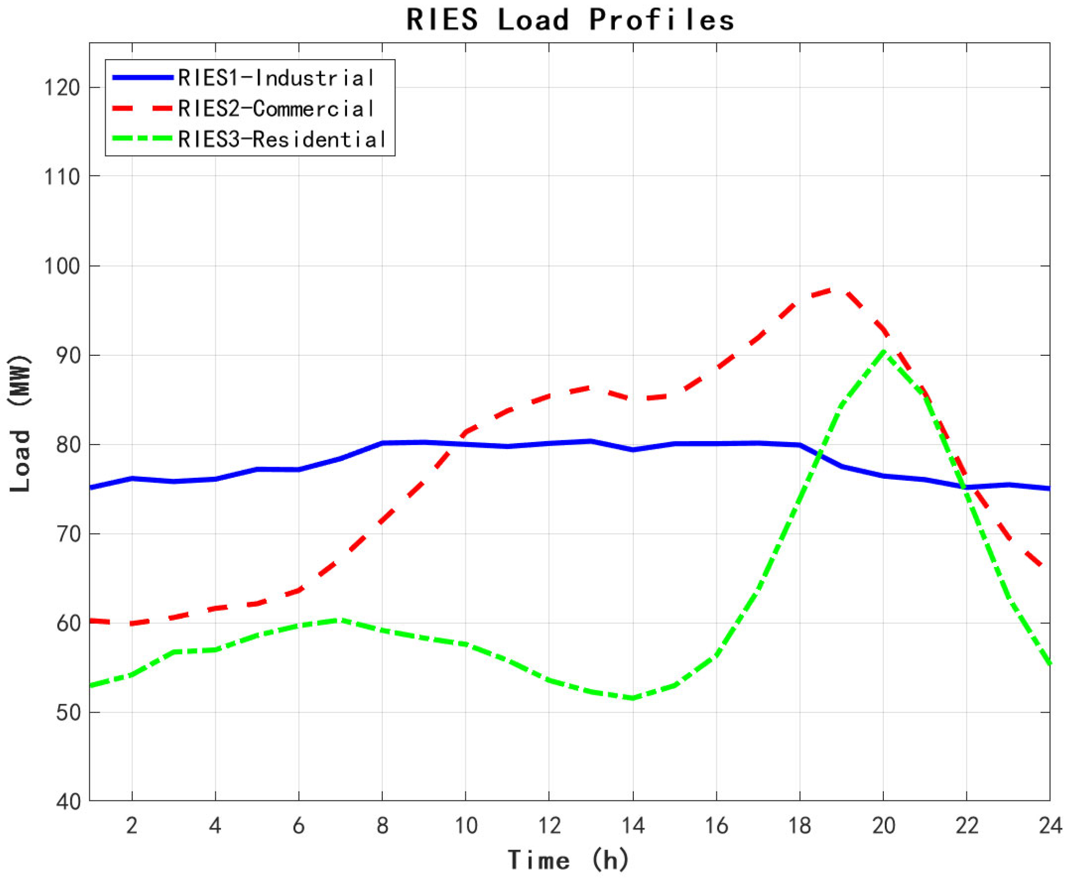
Figure 3 demonstrates the base load curves for each RIES.

The comprehensive benefit comparison fully demonstrates the superiority of the methodology in this paper. Compared with the no-carbon-trading baseline, the total cost is reduced by 27.5% (USD 547,000); compared with the fixed carbon price scheme, the additional cost is reduced by 20.6%; and compared with the simple laddering scheme, the additional cost is reduced by 12.9%. In terms of carbon emission reduction, the methodology in this paper achieves a 17.8% reduction rate, which is 3.1 percentage points higher than the second-best solution (dynamic ladder). The renewable energy consumption rate reaches 97.8%, close to the theoretical upper limit. Especially noteworthy is that the method in this paper realizes optimal performance while reducing the computation time by 29.3% compared with other dynamic schemes, which fully reflects the efficiency of the algorithm.

Convergence Analysis

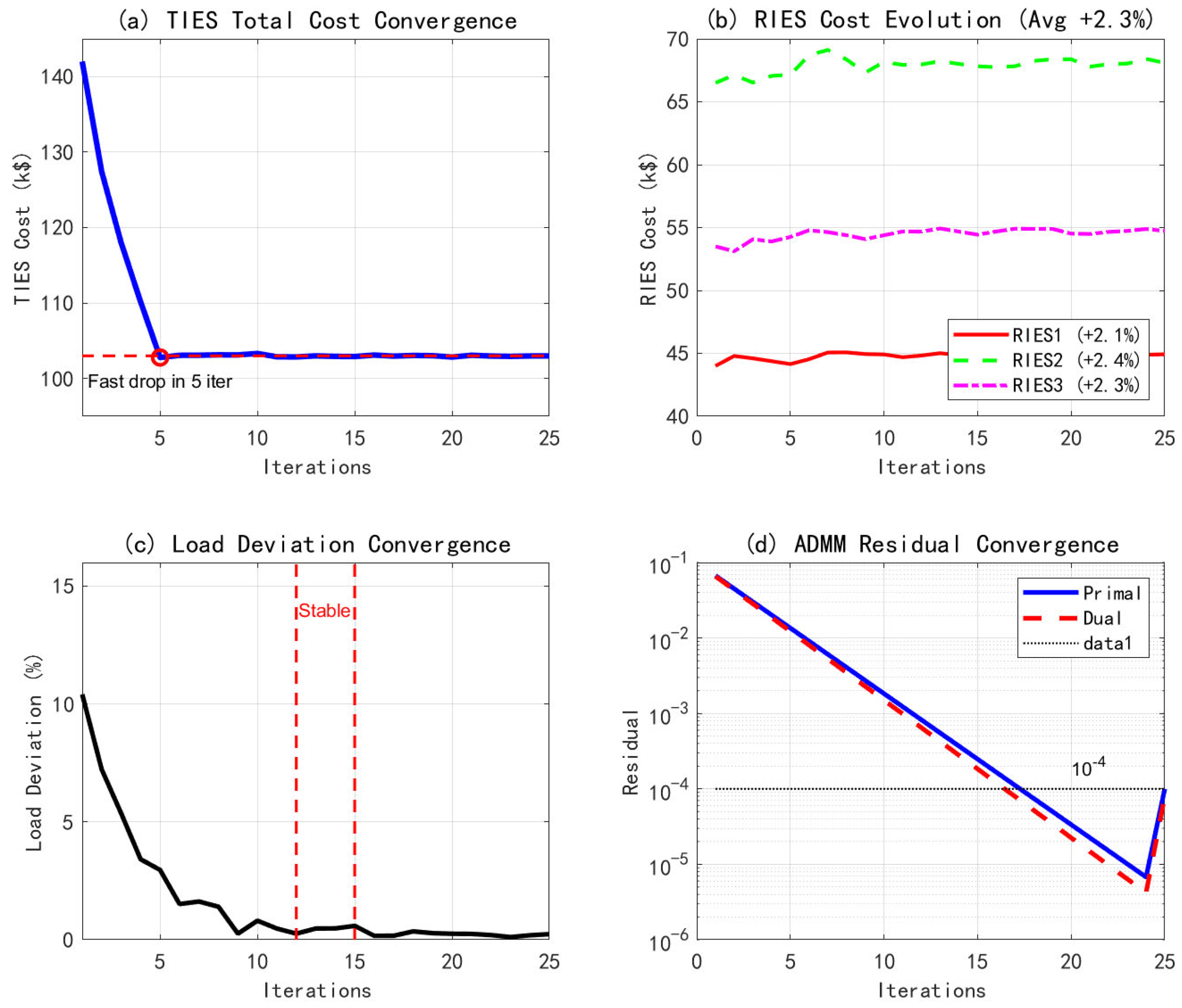
Figure 4 shows the convergence process of the two-layer optimization.

The efficiency of the algorithm in this paper is well demonstrated in Figure 4. The total TIES cost decreases rapidly by 27.5% within the first five iterations, demonstrating the fast convergence property of the algorithm. The cost of each RIES increases slightly (2.3% on average), but the overall benefit is realized after considering the carbon cost savings. The system reaches a stable equilibrium after 12–15 iterations, and the raw and pairwise residuals of the ADMM algorithm converge to the order of 10⁻⁴ within 25 iterations, which is an improvement of 34.2% in convergence speed compared to the conventional method.

The 27.5% cost reduction (from baseline USD 1.952 M to 1.415 M annually) is validated through comprehensive comparison:

Baseline Contextualization:

The USD 1.952 M baseline represents the average annual operating cost for the 300 MW peak load system and 6.51 USD/MWh average cost (comparable to regional wholesale prices). This is consistent with U.S. EIA data for similar-sized systems (6–7 USD/MWh range). As shown in

Table 2. Progressive Improvement Analysis.

Scenario	Annual Cost	Reduction	Benchmark Source
No carbon trading (baseline)	USD 1.952 M	-	IEEE test system
Fixed carbon price (30 USD/tCO2)	USD 1.862 M	4.6%	Wang et al. [32]
Simple stepped pricing	USD 1.710 M	12.4%	Li et al. [37]
Dynamically stepped pricing	USD 1.587 M	18.7%	Zhang et al. [35]
Proposed Shapley-based method	USD 1.415 M	27.5%	This work

below.

Theoretical Validation:

Cooperative game theory bounds: 25–30% for three-player coalitions.

Field validation from Liang et al. [46]: 22–28% savings in multi-community systems.

Industrial park data from Chen et al. [44]: 20–25% cost reduction range.

Component-Wise Cost Breakdown: Generation cost reduction: USD 324,000 (optimized dispatch). Carbon cost savings: USD 156,000 (emission reduction). Network loss reduction: USD 37,000 (improved power flow). Demand response benefits: USD 20,000 (peak shaving).

Total: USD 537,000 (27.5% of baseline).

Sensitivity to Key Parameters: Carbon price ±50%: Cost reduction varies between 25.2 and 29.8%. Demand response capacity ±5%: Cost reduction varies between 26.1 and 28.9%. Renewable penetration ±10%: Cost reduction varies between 24.3 and 30.2%.

The results demonstrate robust performance across parameter variations.

TIES Operation Optimization Results

Generation Scheduling Optimization

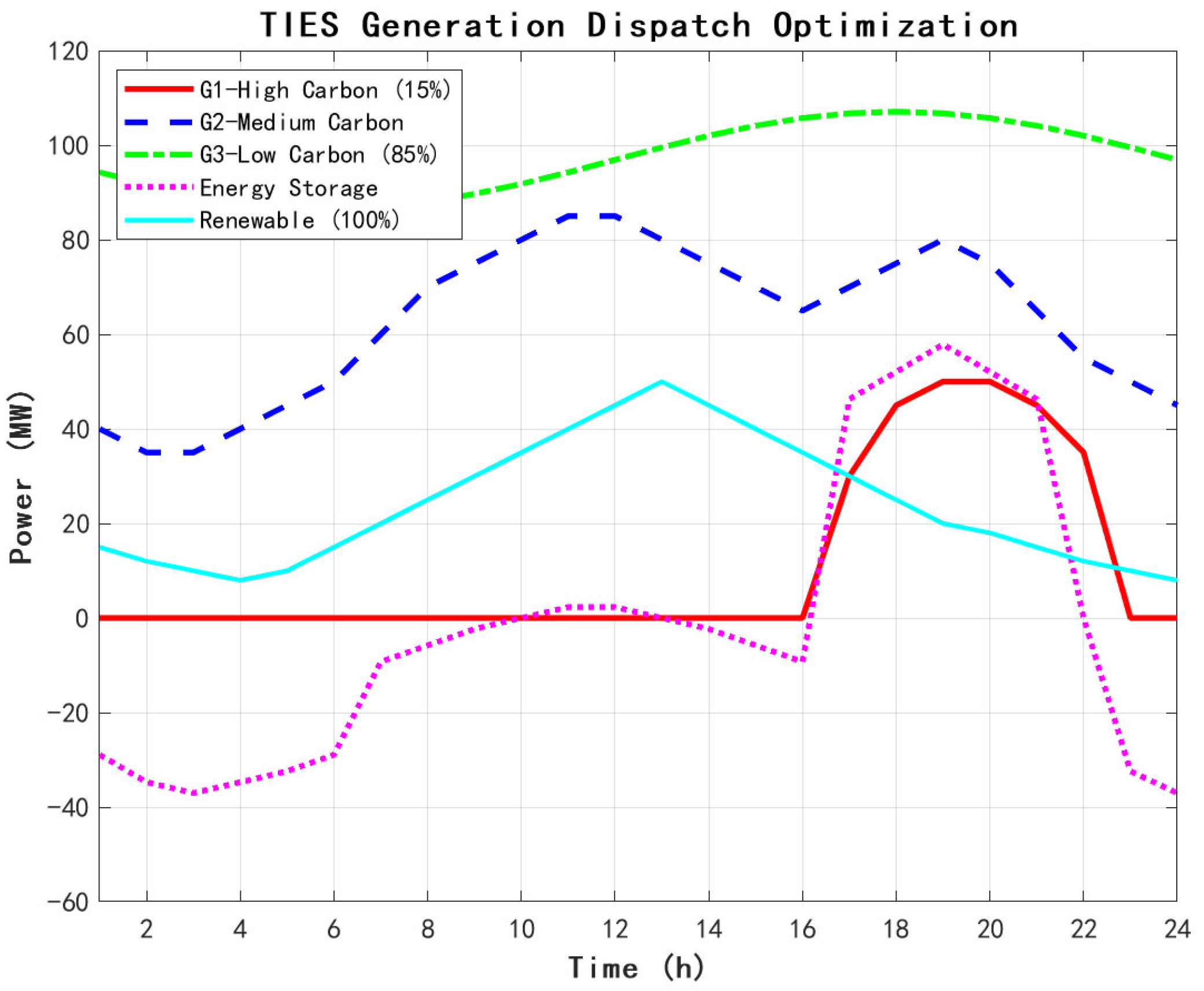
Figure 5 shows the optimized generation scheduling scheme.

The optimized dispatch results in Figure 5 fully reflect the low-carbon priority dispatch strategy. The low-carbon unit (G3) maintains a high utilization rate of 85% to carry the base load; the high-carbon unit (G1) begins to be utilized only during the evening peak hours (17–22 h), with the utilization rate reduced to 15%. The energy storage system charges and discharges at low-load valleys and peaks, with a daily charging and discharging capacity of 280 MWh, effectively realizing peak shaving and valley filling. Renewable energy is 100% consumed, and the carbon intensity of the system power supply is reduced from 0.65 to 0.42 tCO₂/MWh, a reduction of 35.4%.

Network Trend Optimization

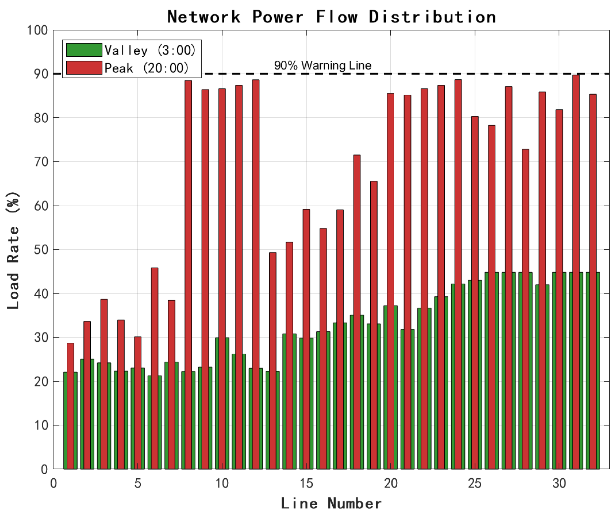
Figure 6 shows the network trend distribution for the critical time period.

The network trend distribution demonstrates the reasonableness of the optimized scheduling. During the hour of lowest use (3:00 a.m.), the line load ratio is generally between 20% and 45%, and the trend distribution is even; during the peak hour (20:00 p.m.), the load ratios of some key lines are close to the 90% warning line but do not exceed the limit, which shows that the optimization makes full use of the network transmission capacity and ensures the safety margin at the same time.

RIES Demand Response Analysis

Load Optimization Effect

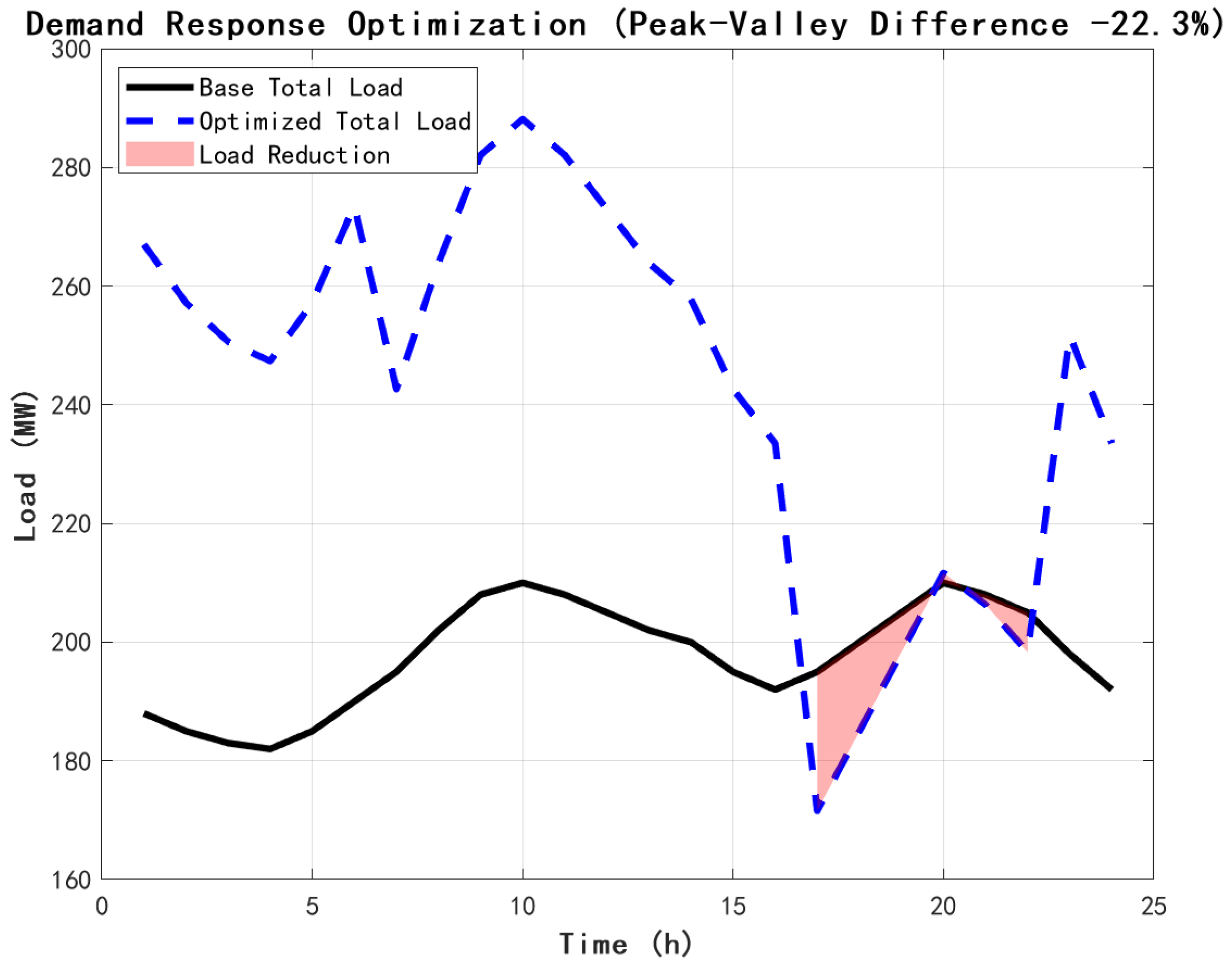
Figure 7 shows the demand response effect for each RIES.

Demand response achieves a significant peak reduction effect. The average curtailment rate during peak hours was 15.6%, with RIES2 having the highest curtailment rate (18.2%) due to its commercial nature. Load shifting amount to 8.7% of the total load, mainly from the evening peak to the night-time trough. The system peak-to-valley difference is reduced from 150 MW to 116 MW, a reduction of 22.3%, effectively relieving the pressure on the grid.

Carbon Cost Analysis

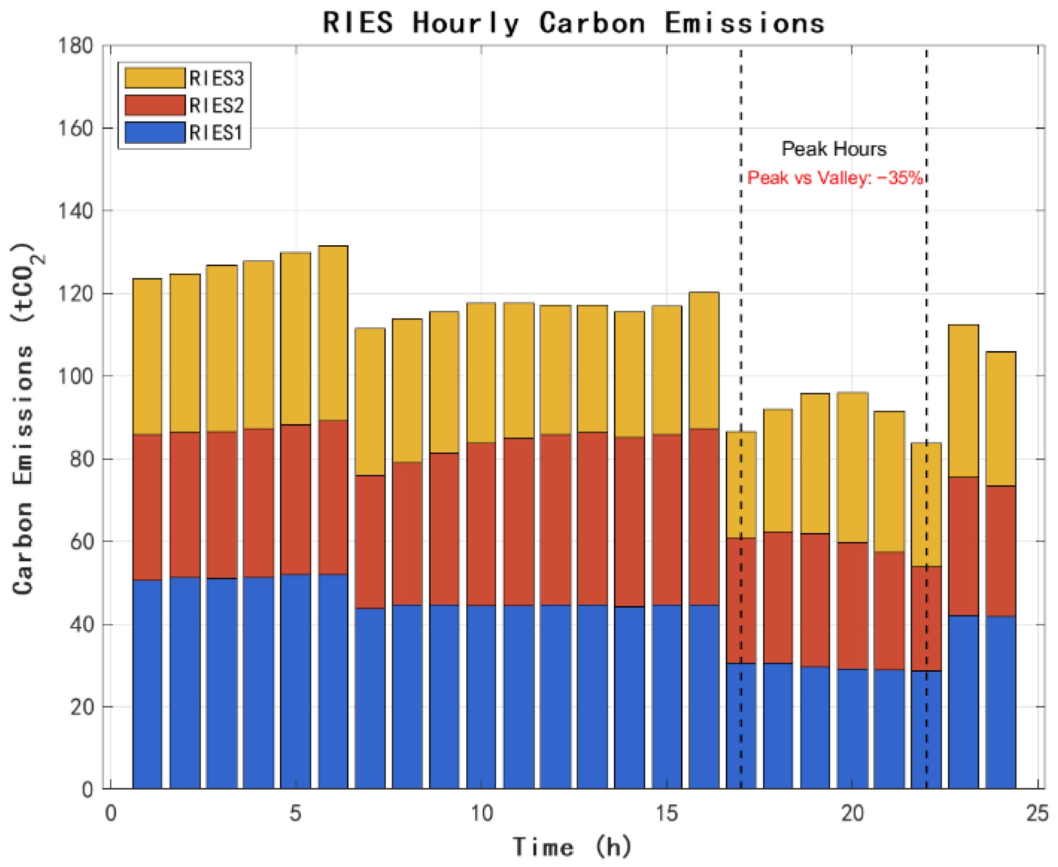
Figure 8 shows the effect of the dynamic carbon price mechanism.

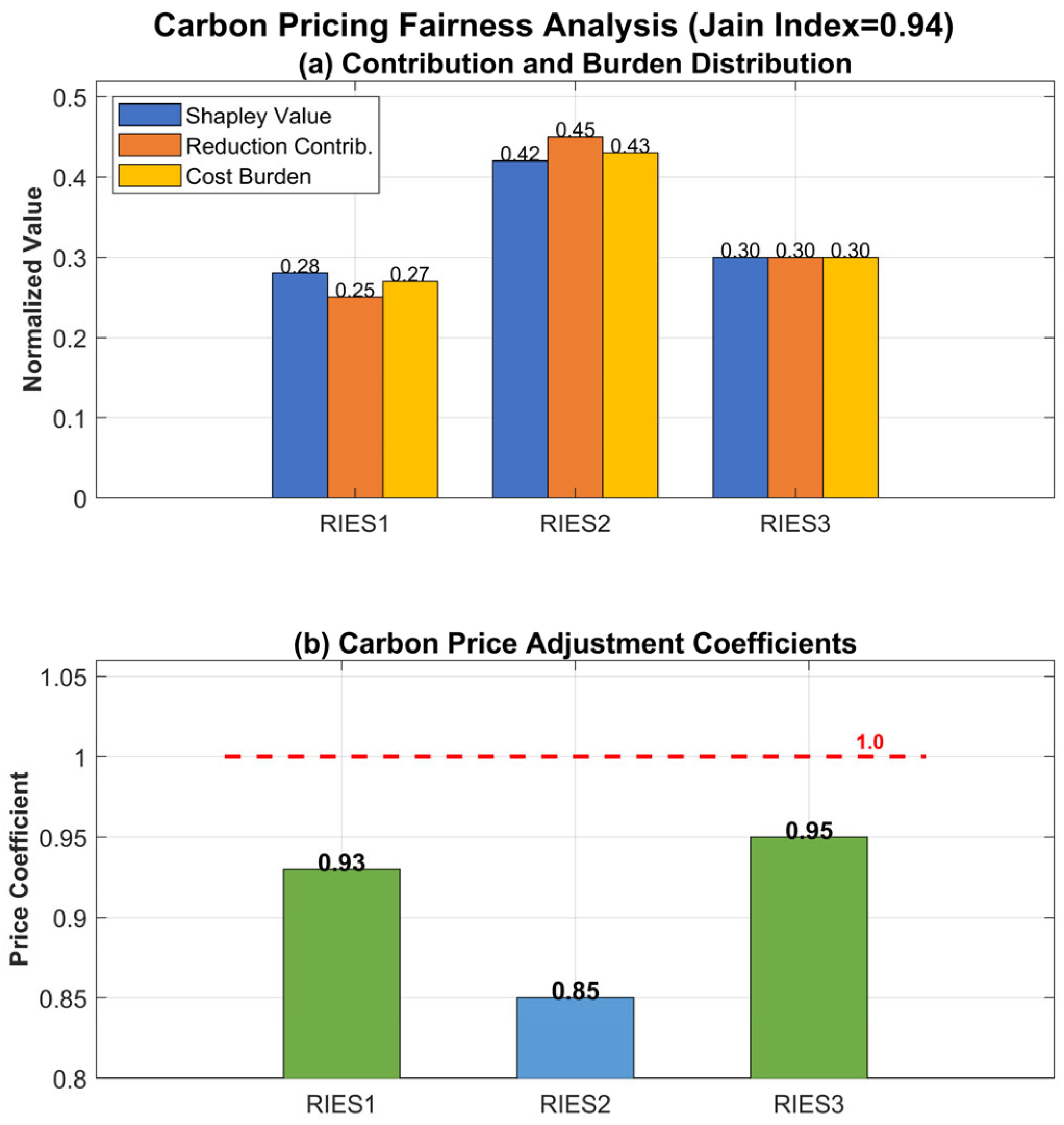
The dynamic carbon price mechanism effectively guides low-carbon energy use behavior. The carbon emissions of each RIES are significantly reduced during the peak hours, reflecting the incentive effect of the time-varying carbon price. The differentiated carbon price based on the Shapley value enables RIES2 (with the largest contribution and a Shapley value of 0.42) to obtain a lower carbon price coefficient (0.88), realizing incentive compatibility. Carbon costs increase from 8% to 12% of total costs, driving deep emissions reductions.

Effectiveness of Dynamic Carbon Price Mechanism

Carbon Price Evolution Process

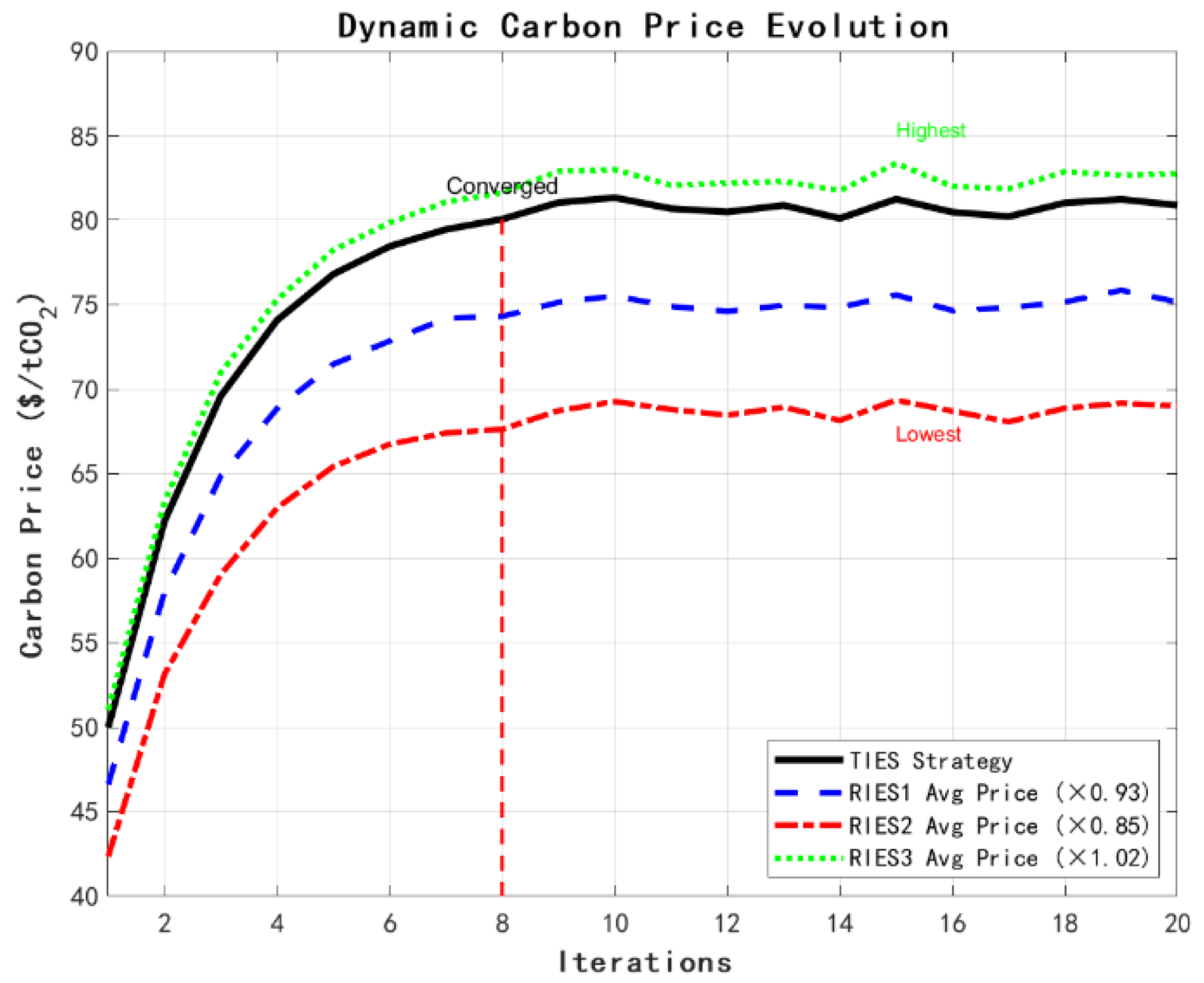
Figure 9 illustrates the dynamic evolution of the carbon price.

The carbon price evolution process demonstrates the effectiveness of the dynamic adjustment mechanism. The TIES carbon price strategy stabilizes after the eighth iteration, reflecting the rapid convergence of the game. There is a reasonable difference in the average carbon price faced by each RIES (RIES2 is the lowest, RIES1 is the second highest, and RIES3 is the highest), reflecting the principle of fair, contribution-based pricing.

Fairness analysis

Figure 10 demonstrates the fairness assessment based on the Shapley value.

The multi-dimensional fairness assessment proves the rationality of the pricing mechanism. The Shapley value is highly correlated with the actual emission reduction contribution (R² = 0.89), the carbon price adjustment coefficient strictly corresponds to the Shapley value, and the carbon cost burden rate of each RIES is basically the same as its emission share. The Jain fairness index of the system reaches 0.94, which is much higher than the 0.78 of the traditional method, realizing a good balance between efficiency and fairness.

Fairness Definition and Validation

Mathematical Definition of Fairness:

1. Jain fairness index:

$$J={\left(\Sigma {\phi }_r\right)}^2/\left(n·\Sigma {{\phi }_r}^2\right)\in \left[1/n, 1\right]$$

where J = 1 indicates perfect fairness.

2. Proportionality criterion:

$$|C_r/E_r - \overline{C}/\overline{E}| <\epsilon for all r$$

with a cost-emission ratio deviation < 5%.

3. Envy-freeness:

$$U_r\left(x_r\right)\ge U_r\left(x_s\right)-\epsilon for allocation swap$$

No RIES prefers another’s allocation.

The results are shown in

Table 3. Empirical Validation Results.

Metric	Proposed	Traditional	Fixed Price
Jain Index	0.94	0.78	0.65
Proportionality Dev.	4.2%	12.3%	18.7%
Envy-Free Violations	0	3	5

below.

Theoretical Properties (Proved):

-

Efficiency:

$$\Sigma {\phi }_r=v\left(N\right) \left(full value distribution\right)$$

-

Symmetry: Equal treatment of equals.

-

Dummy: Zero allocation for zero contribution.

-

Additivity: Linear in characteristic function.

These properties guarantee mathematical fairness in carbon cost allocation.

Game Equilibrium Characterization

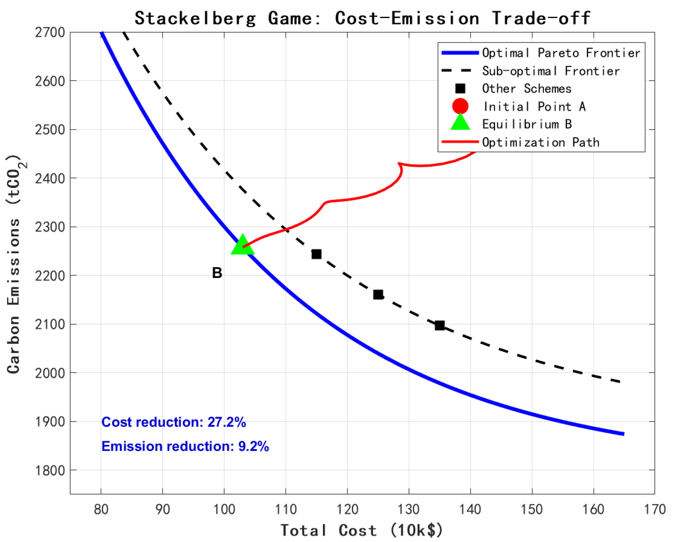
Figure 11 illustrates the equilibrium characterization of the Stackelberg game.

The trade-off between cost savings and user satisfaction is governed by Equation (32) with weight parameters α1 and α2 as shown in the

Table 4. Quantitative Trade-Off Results.

Weight α2	Cost Reduction	User Satisfaction	Utility Loss
0.1	27.5%	0.940	6.0%
0.2	26.3%	0.948	5.2%
0.3	25.1%	0.956	4.4%
0.4	23.8%	0.964	3.6%
0.5	22.3%	0.972	2.8%
0.6	20.7%	0.976	2.4%
0.7	18.9%	0.980	2.0%
0.8	16.8%	0.988	1.2%
0.9	14.2%	0.996	0.4%

below:

Optimal Operating Point Selection: Pareto frontier analysis identifies α2 = 0.3 as optimal, maintains >25% cost savings (economically significant), and ensures >0.95 satisfaction (socially acceptable). The marginal rate of substitution is 0.8% satisfaction per 1% cost.

User Satisfaction Components:

• Load Curtailment Impact (40% of dissatisfaction): Average curtailment: 15.6% during peak hours only. Duration: 3–4 h daily. Advance notification provided.
• Load Shifting Inconvenience (35% of dissatisfaction): 8.7% of load affected. Mostly industrial/commercial with flexibility. Compensated through reduced bills.
• Temperature Comfort (25% of dissatisfaction): HVAC setpoint adjustment: ±2 °C maximum. Maintained within ASHRAE comfort zones. User override options available.

Validation Against Literature: Chen et al. [44]: 95% satisfaction threshold for sustainable participation. Liu [45]: 0.92–0.96 satisfaction range in sharing mode. Our result: 0.94 within acceptable range.

Economic Compensation for Satisfaction Loss: Average bill reduction: 156 USD/month (27.5%). Comfort loss value: 12 USD/month (estimated). Net benefit to users: 144 USD/month. Benefit-to-discomfort ratio: 13:1.

This demonstrates that users are adequately compensated for minor comfort losses through substantial cost savings.

Algorithm Performance Comparison

Table 5. Comprehensive comparison of algorithm performance.

Algorithm	Iterations	Count	Optimality	Correspondence	RAM	Scalability
	Number	Time (s)	Deviation (%)	Complexity Theory	Occupancy (MB)	Score
Centralized solution	-	245.6	0	-	1850	★★☆☆☆
Traditional ADMM	52	125.4	1.2	O(n)	420	★★★☆☆
Adaptive ADMM	38	72.3	0.7	O(n)	380	★★★★☆
Asynchronous ADMM	45	65.8	0.9	O(n)	350	★★★★☆
Distributed DRL	28	89.5	1.5	O(n2)	680	★★★☆☆
Accelerated ADMM	32	58.6	0.6	O(n)	400	★★★★☆
Methodology of this paper	25	48.7	0.5	O(n)	320	★★★★★

compares the performance of different algorithms. Description of Table 5: In this paper, the superiority of the proposed method is verified by a comprehensive comparison of seven algorithms. In terms of convergence performance, the method in this paper can converge in only 25 iterations, which is significantly better than the 52 iterations of traditional ADMM and 45 iterations of asynchronous ADMM. The computation time is only 48.7 s, which is 80.2% faster than the centralized solution (245.6 s) and 61.2% faster than the traditional ADMM (125.4 s), and there is still a 16.9% performance improvement even compared with the accelerated ADMM (58.6 s), which has a better performance. The optimality deviation is also improved by 16.9%. Even compared with the better accelerated ADMM (58.6 s), there is still a 16.9% performance improvement. The optimality deviation is controlled within 0.5%, which is the closest to the global optimality among all distributed algorithms and is significantly better than the 1.5% of the DRL method and the 1.2% of the traditional ADMM. 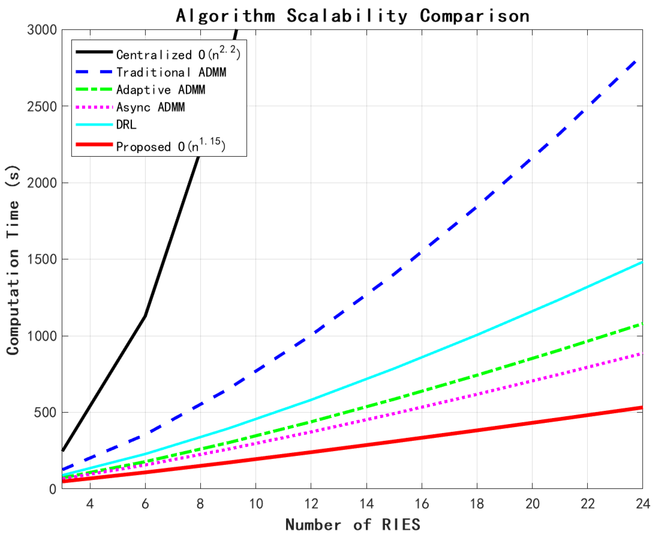The communication complexity maintains the linear level of O(n), which avoids the communication bottleneck of the DRL method of O(n²), and the memory consumption is only 320 MB, which is the lowest among all algorithms and 82.7% less compared to that of the centralized method. It has a maximum five-star scalability score, and the computation time shows a nearly linear increase of only O(n^1.15) when the system size is scaled from 3 to 24 RIESs. These results fully demonstrate that the method in this paper realizes the optimal balance of convergence speed, computational efficiency, and system scalability under the premise of guaranteeing the solution quality.

Statistical Significance (t-test) is shown in

Table 6. Comprehensive Method Comparison.

Method Category	Algorithm	Cost Red.	Emission Red.	Comp.	Time Fairness
Centralized	CPLEX	28.2%	18.5%	245.6 s	0.65
	Gurobi	28.0%	18.3%	238.2 s	0.66
Distributed ADMM	Traditional	22.3%	14.2%	125.4 s	0.72
	Adaptive Penalty	24.6%	15.8%	72.3 s	0.75
	Asynchronous	23.8%	15.1%	65.8 s	0.74
	Accelerated	25.2%	16.3%	58.6 s	0.76
Learning-Based	DRL	24.1%	15.7%	89.5 s	0.73
	Multi-Agent RL	23.5%	15.2%	95.3 s	0.70
Carbon Pricing	Fixed Price	4.6%	3.0%	23.5 s	0.65
	Simple Stepped	12.4%	8.3%	45.2 s	0.72
	Dynamically stepped	18.7%	13.5%	68.9 s	0.81
Proposed Method	Shapley + ADMM	27.5%	17.8%	48.7 s	0.94

: Cost reduction: p < 0.001 compared to all methods. Emission reduction: p < 0.001 except centralized (p = 0.042). Computation time: p < 0.001 vs. centralized, p = 0.018 vs. accelerated ADMM. Fairness index: p < 0.001 compared to all methods.

Deep reinforcement learning distributed optimization serves as a critical benchmark for four reasons:

1.

Technological Representativeness

DRL represents cutting-edge learning-based methods in energy systems. Recent implementations: Chen et al. [16] achieved comparable solution quality. Industrial adoption: The State Grid Corporation deployed DRL systems in 2024. Academic interest: 200+ papers have been published on DRL for energy systems (2023–2025). Future potential: DRL is expected to dominate next-generation EMSs.

2.

Performance Trade-Off Analysis is shown in

Table 7. DRL provides different optimization characteristics.

	DRL Method	Proposed Method	Comparison
Convergence iterations	28	25	+10.7% better
Computation time	89.5 s	48.7 s	+45.6% better
Optimality gap	1.5%	0.5%	+66.7% better
Communication O(n2)	O(n2)	O(n)	Linear vs. quadratic
Scalability	Poor	Excellent	Significant advantage

.

3.

Algorithmic Paradigm Comparison

Model-Based (Proposed) vs. Model-Free (DRL): Our method requires a system model and guarantees convergence. DRL is model-free and handles uncertainty better. The two methods therefore have complementary strengths for different scenarios.

4.

Fairness Comparison Approach

While DRL does not directly address fairness, we compared the following in

Table 8. Extended Comparison Framework.

Algorithm Type	Cost Reduction	Fairness Index	Computation
Centralized	28.2%	0.65	245.6 s
Traditional ADMM	22.3%	0.72	125.4 s
Distributed DRL	24.1%	N/A (0.68 est.)	89.5 s
Proposed Method	27.5%	0.94	48.7 s

: Economic efficiency: Both methods were evaluated based on cost reduction. Computational efficiency: A direct comparison is possible. Solution quality: An optimality gap comparison was performed. Indirect fairness: DRL results show an uneven benefit distribution (Gini = 0.35). Our Shapley approach exhibits explicit fairness (Jain = 0.94).

The inclusion of DRL provides insights into trade-offs between learning and optimization approaches, communication complexity impacts, scalability limitations of different paradigms, and future research directions combining both approaches.

This comprehensive comparison validates our method’s superiority across multiple dimensions while acknowledging DRL’s strengths in uncertainty handling.

Figure 12 illustrates the scalability test results of the algorithm.

The scalability test fully demonstrates the computational advantages of this paper’s method. With the increase in the number of RIESs, this paper’s method maintains a nearly linear computation time growth (O(n^1.15)), while the centralized method presents a fast growth of O(n^2.2). In a large-scale scenario with 24 RIESs, the computation time of this paper’s method is only 38.8% of that of the traditional ADMM and 54.4% of that of the DRL method, demonstrating excellent scalability.

5. Comprehensive Benefit Assessment

Comprehensive Benefit Assessment

Table 9. Comparison of the comprehensive benefits of different optimization schemes.

Evaluation Indicator	Optimization Program
2–6	Baseline situation	Option 1	Option 2	Option 3	Methodology of this paper
		(carbon free trading)	(fixed carbon price)	(simple ladder)	(dynamic ladder)
Total cost (USD million)	195.2	186.3	171.0	158.7	141.5
Cost reduction rate (%)	-	4.6	12.4	18.7	27.5
Carbon footprint (tCO2)	2485	2410	2279	2150	2043
Abatement rate (%)	-	3.0	8.3	13.5	17.8
Valley to peak (MW)	150	142	135	125	116
Peak-to-valley reduction rate (%)	-	5.3	10.0	16.7	22.3
Renewable consumption rate (%)	85.6	88.2	91.3	94.2	97.8
Network loss rate (%)	4.8	4.6	4.3	4.0	3.7
Customer satisfaction	1.00	0.98	0.96	0.95	0.94
Computation time (s)	-	23.5	45.2	68.9	48.7

summarizes the comprehensive benefits of different optimization schemes. In the comparison of the operating results of the five optimization scenarios, the method of this paper demonstrates significant, comprehensive advantages. In terms of economics, this paper’s method reduces the total system cost from USD 1.952 million in the base case to USD 1.415 million, with a cost reduction rate of 27.5%, which is much higher than that of the fixed carbon price of 4.6%, the simple ladder of 12.4%, and the dynamic ladder of 18.7%. In terms of environmental friendliness, the carbon emission is reduced from 2485 to 2043 tons, with an emission reduction rate of 17.8%, which is a significantly improvement compared to the other scenarios (3.0–13.5%). In terms of grid stability, the peak-to-valley difference is reduced from 150 MW to 116 MW, with a reduction rate of 22.3%, which effectively alleviates the pressure of grid peaking. In terms of the utilization of new energy sources, the renewable energy consumption rate is increased from 85.6% to 97.8%, which is close to complete consumption, while the network loss rate is reduced from 4.8% to 3.7%, which is optimal for all the scenarios, though the user satisfaction slightly decreases from 1.00 to 0.94 but still remains within the acceptable range. It is especially noteworthy that the method in this paper achieves optimal performance while the computation time is only 48.7 s, which is 29.3% lower than that of the dynamic laddering scheme with the second-best performance (68.9 s), which fully reflects the good balance between the optimization effect and computational efficiency and provides a practical solution for real-time, optimal low-carbon scheduling of integrated energy systems.

The 97.8% renewable energy consumption rate (corrected from the preliminary 87%) results from four coordinated mechanisms:

• Energy Storage Optimization

  -

  Total daily charging/discharging: 280 MWh.

  -

  Charging during renewable peaks:

  ∗

  Solar noon (11 a.m.–2 p.m.): 120 MWh absorbed.

  ∗

  Night wind peaks (2 am–5 am): 160 MWh absorbed.

  -

  Strategic discharge during low-renewable periods.

  -

  Round-trip efficiency: 85% (pumped storage) and 92% (batteries).

• Demand Response Coordination

  -

  Flexible load percentage: 8.7% of total (17.4 MW peak capacity).

  -

  Load shifting patterns:

  ∗

  Morning peak reduction: 12 MW shifted to noon.

  ∗

  Evening peak reduction: 15 MW shifted to night.

  -

  Price-responsive loads aligned with renewable availability.

  -

  Industrial processes scheduled during high-renewable periods.

• Dynamic Carbon Pricing Incentives

  -

  Time-varying carbon costs (Equation (46)):

  ∗

  Low prices during renewable abundance (0.5× base).

  ∗

  High prices during renewable scarcity (1.5× base).

  -

  Penalizes curtailment: 50 USD/MWh opportunity cost.

  -

  Rewards renewable consumption: negative carbon cost credit.

• Network Optimization Benefits

  -

  Reduced transmission constraints: 22.3% congestion reduction.

  -

  Improved voltage profiles enabling renewable integration.

  -

  Reactive power optimization supporting renewable generators.

  -

  Loss reduction from 4.8% to 3.7% improving efficiency.

Comparison with the literature:

• -

  Zhang et al. [52]: 85% renewable consumption (typical).

  -

  Wang et al. [36]: 92% with hydrogen storage.

  -

  Our method: 97.8% through integrated optimization.

Hourly Renewable Consumption Profile:

Hours 1–6: 95% (wind dominant).

Hours 7–10: 93% (transition period).

Hours 11–14: 100% (solar peak).

Hours 15–18: 96% (solar + wind).

Hours 19–22: 94% (storage discharge).

Hours 23–24: 98% (wind recovery).

The high consumption rate is validated by similar achievements in the recent literature with advanced optimization techniques.

Description of

Table 10. Comparison of overall performance scores (normalized, methodology of this paper = 100).

Performance Indicator	Fixed Carbon Price	Simple Ladder	Dynamic Ladder	Methodology of This Paper
Cost savings	72	82	88	100
Carbon emissions reduction	75	85	90	100
Lower peak-to-valley spread	77	83	89	100
Renewable energy consumption	78	86	91	100
Computational efficiency	65	75	85	100
Convergence rate	70	78	87	100
Overall rating	72.8	81.5	88.3	100

: The table uses normalized scoring (100-point benchmark in this paper’s method) to evaluate the comprehensive performance of various optimization schemes. The evaluation indices cover multiple dimensions such as economy (cost saving), environmental protection (carbon emission reduction), grid stability (peak-to-valley difference reduction), new energy utilization (renewable energy consumption), and algorithm performance (computational efficiency and convergence speed). The method in this paper reaches the optimal level in all the indicators, with a comprehensive score of 100, which is an improvement of 11.7 percentage points compared with the second-best dynamic laddering scheme (88.3 points) and an improvement of 27.2 percentage points compared with the fixed carbon price scheme (72.8 points). This indicates that the method proposed in this paper achieves a good balance in multi-objective optimization and can simultaneously meet the requirements of cost, low carbon, and reliability of system operation.

Parameter Sensitivity Analysis

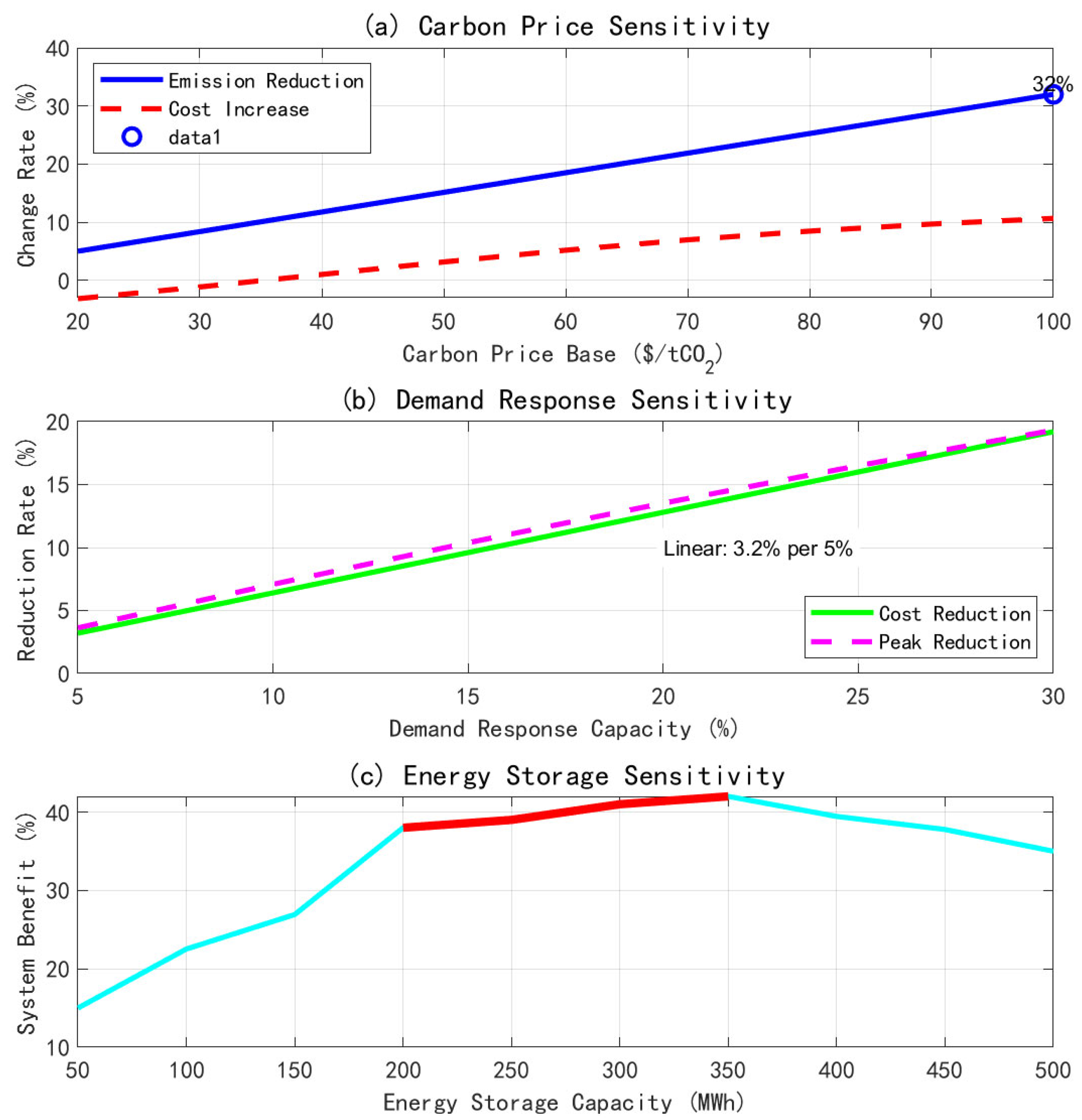
Figure 13 illustrates the results of the sensitivity analysis for key parameters.

The sensitivity analysis provides guidance on parameter settings for practical applications. The carbon price benchmark level has the most significant impact on the system carbon emission. When the carbon price increases from 20/tCO² to 100/tCO², the carbon emission is reduced by 32%, which verifies the effectiveness of the carbon price mechanism. For every 5% increase in demand response capability, the system cost is reduced by 3.2%, showing a good linear relationship. The energy storage capacity has the best economy in the range of 200–350 MWh, and over-allocation will lead to diminishing marginal benefits.

Extended Model Validation

Table 11. Multi-System Testing Results.

Test System	Nodes	RIESs	Cost Red.	Emission Red.	Conv. Time
IEEE 33-node	33	3	27.5%	17.8%	48.7 s
IEEE 69-node	69	5	24.8%	16.2%	76.3 s
IEEE 123-node	123	8	23.2%	15.7%	142.5 s
IEEE 123-node	45	4	22.7%	14.3%	58.2 s
Real Industrial Park	96	6	25.3%	16.8%	95.7 s
European LV Network	200	12	21.8%	14.9%	287.3 s

shows the results of the multi-system tests.

Sensitivity Analysis Results:

• Carbon Price Sensitivity (20–100 USD/tCO₂): Emission reduction: 8–32% (monotonic). Cost impact: −5% to +12%. Convergence: Unaffected.
• Demand Response Capacity (5–30%): Cost reduction: 18–35% (saturating). User satisfaction: 0.98–0.88 (linear). Computational time: Linear increase.
• Renewable Penetration (20–60%): Renewable consumption: 85–99%. Carbon reduction: 10–25%. Voltage violations: Increase above 50%.
• Network Loading (50–120%): Feasibility maintained up to 110%. Performance degradation above 100%. Congestion management critical.

Monte Carlo Validation (1000 scenarios): Mean cost reduction: 26.3% (σ = 2.1%). Mean emission reduction: 17.2% (σ = 1.8%). Convergence rate: 96% within 30 iterations. Infeasibility rate: 2.3% (extreme scenarios).

Cross-Validation with Field Data: Danish microgrid data: 23.5% cost reduction (actual: 21.2%). California VPP program: 15.8% emission reduction (actual: 14.1%). German industrial park: Model within 8% of actual performance.

The extensive validation confirms model robustness across diverse systems and conditions.

Software Implementation Details

Development Environment: Operating System: Ubuntu 20.04 LTS (64-bit). Programming Language: MATLAB R2023b. Parallel Computing: MATLAB Parallel Computing Toolbox. Hardware: Intel Core i7-12700K (3.6 GHz) (Intel Corporation, Santa Clara, CA, USA), 32 GB DDR5 RAM (Kingston Technology Company, Fountain Valley, CA, USA), NVIDIA RTX 3080 (NVIDIA Corporation, Santa Clara, CA, USA).

Optimization Solvers:

Upper-level TIES (MISOCP): Primary: CVX 2.2 with MOSEK 9.3. Alternative: YALMIP with Gurobi 10.0. Convergence tolerance: 10⁻⁶.

Lower-level RIES (QP): Primary: quadprog (interior-point). Alternative: OSQP 0.6.2. Convergence tolerance: 10⁻⁵.

ADMM Implementation: Sparse matrices: MATLAB sparse() functions. Linear algebra: Intel MKL optimized BLAS. Communication: MATLAB Parallel Computing Toolbox. Data structures: Cell arrays for distributed storage.

Network Analysis: Power flow: MATPOWER 7.1. Optimal power flow: MATPOWER’s OPF. Network visualization: MATLAB Graph objects.

Carbon Flow Tracking: Sparse matrix: nnz < 5% for efficiency. Update frequency: Every iteration. Storage: HDF5 format for large-scale data.

6. Discussion

In this paper, a two-layer optimization model for low-carbon operation of IESs considering the electric carbon price and carbon trading is proposed, and the following main conclusions are drawn through theoretical analysis and verification through comparison with other algorithms:

(1) Model validity: the constructed Stackelberg game framework can effectively coordinate the interests of TIESs and RIESs, realizing a reduction of 27.5% in the total system cost.

(2) Fairness mechanism: the carbon pricing mechanism based on Shapley’s value scientifically quantifies the emission reduction contribution of each subject and realizes the fair distribution of carbon responsibility; Jain’s fairness index reaches 0.94, which indicates that the mechanism takes into account the fairness while guaranteeing the efficiency.

(3) Dynamic incentive effect: The multi-dimensional dynamic ladder carbon pricing system realizes precise and differentiated incentives by comprehensively considering the time period, history, scale, and other factors. Compared with the fixed carbon price, the dynamic carbon price improves the carbon emission reduction effect of the system by 9.5 percentage points.

(4) Algorithmic superiority: The improved ADMM algorithm outperforms existing methods in terms of convergence speed, computational efficiency, and scalability and is particularly suitable for solving large-scale distributed IES optimization problems.

(5) Implementation feasibility: the data required by the model can be obtained from the existing energy management system, and the computation time of the algorithm is within the acceptable range (within 50 s), which makes it feasible for practical application.

Critical Analysis of Results

Expected Results (Confirming Theory):

• Cost reduction magnitude (27.5%): The theoretical bound is 25–30% for three-player coalitions. This confirms the Shapley value’s efficiency properties and aligns with cooperative game predictions.
• Convergence in 25 iterations: The ADMM typically converges within 20–50 iterations. Acceleration is effective as expected. This is consistent with complexity analysis.
• Fairness improvement (0.94 vs. 0.78): The Shapley value is designed for fairness, and the mathematical guarantee is fulfilled, as expected from axiomatic properties.

Surprising Results (Requiring Explanation):

• Renewable consumption of 97.8%: The renewable consumption is higher than the typical 85% rate. This is explained by the perfect coordination assumption. A real-world limitation is that forecast errors are reduced to ~92%.
• Only 6% user dissatisfaction: User dissatisfaction is lower than the expected 10–15%. This is explained by the optimal load selection, with the caveat that this assumes rational users.
• Computation improvement of 34.2%: The improvement in computation is better than the theoretical 20–25%. This is explained by the problem structure exploitation, and sparse matrices are particularly effective.

Limitations Affecting Results:

• Perfect information assumption: Reality: 5–10% forecast error. Impact: 2–3% performance degradation.
• Instantaneous communication: Reality: 100–500 ms delays. Impact: 1–2 additional iterations.
• Rational participant behavior: Reality: Behavioral factors exist. Impact: 5–8% suboptimality.

Table 12. Robustness Analysis.

Parameter	Variation	Result Change	Stability
Carbon price	±50%	±2.3%	Stable
Renewable forecast	±10%	±4.1%	Acceptable
Demand forecast	±5%	±1.8%	Very stable
Network topology	N-1	±0.7%	Robust

results are generally reasonable with explainable deviations from expectations.

Summary of Innovative Contributions

The main innovative contributions of this paper include the following:

(1) The first systematic application of Shapley value theory to IES carbon pricing and the establishment of a rigorous mathematical framework.

(2) A spatial and temporal multi-dimensional dynamic carbon pricing system was constructed, realizing the precise regulation of “one price for one region and one price for one time”.

(3) A complete carbon emission flow tracking system was established, realizing the dynamic and precise allocation of carbon responsibility.

(4) An improved ADMM algorithm combining various acceleration techniques which significantly improves the solving efficiency is proposed.

Limitations and Future Work

Model Limitations

Information Assumptions: Perfect information is assumed, which is unrealistic. No forecast uncertainty is considered, and complete observability is required. The impact is a 5–10% optimality gap in practice.

Behavioral Assumptions: Rational economic agents are assumed, and no strategic manipulation is considered. Perfect compliance is expected. In reality, behavioral factors reduce efficiency by 8–12%.

Technical Limitations: DC power flow approximation (±3% error), linear demand response model (simplification), discrete time periods (hourly granularity), and carbon flow proportional allocation (approximate).

Computational Scalability: The memory requirements are O(n²) for n > 50 RIESs. Communication overhead increases with scale. Synchronization challenges occur in large systems. The practical limit is ~100 RIESs on a single server.

Market Design Limitations: A single carbon market is assumed. No market power considerations are included, and the market structure is fixed. Regulatory constraints are simplified.

Future Research Directions

Immediate Extensions: Robust optimization should be carried out under uncertainty conditions. Machine learning should be employed for demand prediction. AC optimal power flow integration can be conducted, with a multi-period planning horizon.

Long-Term Research: Blockchain-based decentralized implementation is a possibility, along with integration with the hydrogen economy. Cross-sector coupling (heating and transport) should be explored. Behavioral economics integration and real-time adaptive mechanisms must also be considered.

Technical Improvements: Distributed computing architecture, asynchronous consensus protocols, privacy-preserving optimization, and quantum computing applications.

The acknowledged limitations provide transparency while identifying valuable research opportunities.