Article

Machine Learning Insight into the Cooling Intensity of Urban Blue-Green Spaces During Heatwaves

1
International School, Duy Tan University, Da Nang 550000, Vietnam
2
Faculty of Civil Engineering, Duy Tan University, Da Nang 550000, Vietnam
3
Institute of Research and Development, Duy Tan University, 03 Quang Trung, Da Nang 550000, Vietnam
*
Author to whom correspondence should be addressed.
Sustainability 2025, 17(21), 9824; https://doi.org/10.3390/su17219824
Submission received: 9 September 2025 / Revised: 25 October 2025 / Accepted: 28 October 2025 / Published: 4 November 2025
(This article belongs to the Special Issue Urbanization and Environmental Sustainability—2nd Edition)

Abstract

Urban blue-green spaces are essential land cover types that play a critical role in mitigating urban heat stress. However, the cooling performance of these spaces during heatwave events is influenced by a complex interaction of topographical features and landscape configurations. This study examines the spatial variation in cooling intensity (CI) induced by blue-green spaces within the central urban area of Hue City, Vietnam. Land surface temperature in the study area was derived from Landsat 8 satellite imagery captured between 1 May and 30 September 2024, a period marked by record-high heatwaves. The analysis employs an extreme gradient boosting machine (XGBoost version 1.6.2) to quantitatively assess the relationship between CI and the contributing factors for various urban blocks. The XGBoost model demonstrates high predictive accuracy, shown by a coefficient of determination of 0.97. Notably, approximately 92% of predictions yield errors between −1 °C and +1 °C. Interpretation using SHapley Additive exPlanations helps identify primary influencing factors governing the CI. The presented framework presents a robust data-driven approach for evaluating the effectiveness of blue-green spaces in mitigating thermal stress in Hue City. These findings provide practical recommendations for urban planners aiming to enhance thermal comfort in the study area.

1. Introduction

1.1. Research Background and Motivation

Urban areas worldwide are confronted with significant challenges due to climate change, air pollution, and declining public health. Urbanization is accelerating, and it is anticipated that close to 70% of the global population will live in cities by 2050, intensifying the need to address these interrelated issues [1]. At the start of this century, roughly 50% of people were already city dwellers [2]. It is expected that urban land area may increase threefold by 2030 [3], which will produce extensive changes in local and regional climate conditions. As cities expand, effective strategies to manage environmental quality and promote public health become essential priorities for researchers and local authorities.
Particularly in developing countries, rapid urbanization presents major obstacles to achieving urban sustainability. As urban areas grow, natural habitats are frequently disrupted or eliminated due to poor and uncoordinated landscape planning. This fact results in the fragmentation and loss of natural land surfaces. This transformation is often accompanied by rising levels of pollution and habitat degradation, which intensify environmental pressures in cities [4,5,6]. Moreover, natural land covers are increasingly replaced by impervious surfaces; this process contributes to the formation of urban heat islands. The urban heat island (UHI) effect changes the urban microclimate. It makes cities warmer and less comfortable for inhabitants. UHI brings about multiple challenges, including increased energy consumption for building cooling and higher risks of both physical and mental health issues among city residents.
Additionally, recent climate change has caused a rise in the frequency and intensity of extreme weather events [7,8]. Data from the World Health Organization indicate that, between 2000 and 2016, global extreme weather incidents rose by 46%, and the number of vulnerable people exposed to heatwaves grew by 125 million [9]. Extreme heat diminishes physical and cognitive performance as well as impacts mental health [10,11]. As pointed out in [3], approximately 30% of people worldwide now live in regions where temperatures are harmful for human health for at least twenty days each year. In Europe, heatwaves during the summer of 2022 resulted in tens of thousands of heat-related deaths [12]. Accordingly, mitigation of urban heat stress has become a central focus for researchers.
Heat stress in Vietnam’s urban centers has intensified in recent years, largely due to rapid urbanization, changes in land cover, and climate change. Previous works have reported increases in both frequency and intensity of heat stress throughout the country [13,14,15,16]. Pham-Thanh et al. [17] also pointed out that lagged effects of the El Niño–Southern Oscillation (ENSO) are likely major contributors to these patterns. As a consequence, during the hot, humid summer months, climate change has led to more frequent hot days [13]. This escalation in heat stress has sparked concerns about its negative impacts on public health [18,19].
In urban areas, blue-green spaces play a crucial role in reducing the negative impacts of urban heat stress, particularly during heat waves. These areas include water bodies and vegetated land, such as rivers, channels, retention ponds, urban tree canopy, shrubland, and croplands. Blue-green spaces typically maintain lower land surface temperatures compared to built-up areas; this phenomenon is commonly referred to as the cooling island effect [20]. To address the challenges posed by urbanization and climate change, cities are increasingly relying on green infrastructures to harness their cooling benefits and improve the thermal comfort of dwellers [21]. In this context, exploring the factors that govern the cooling intensity (CI) of blue-green spaces could provide essential insights for urban planning and heat stress alleviation [22].
In recent years, developments in remote sensing and machine learning have paved the way for accurate assessment of the CI associated with urban blue-green spaces. The increasing utilization of satellite imagery has expanded possibilities in urban thermal research. Land surface temperature (LST), a critical measure of the urban heat stress, can be derived openly from satellite data. Notably, the assessment of urban thermal via remote sensing is reliable due to a good agreement between the satellite-derived measurements and those obtained from field studies [23]. As a result, remote sensing is highly suitable for large-scale analyses of blue-green infrastructure, especially when integrated with geographic information systems [24].
In addition, machine learning algorithms have demonstrated excellent capability in identifying complex nonlinear relationships among landscape and environmental features [25]; this capability enables them to achieve high prediction accuracy in geospatial modeling of urban land surface temperature [26,27]. Among the machine learning methods, Extreme Gradient Boosting (XGBoost) offers notable advantages for geospatial modeling, including its ability to analyze high-dimensional datasets and capture complex nonlinear relationships among various influencing factors [28,29]. Combined with SHapley Additive exPlanations (SHAP), XGBoost can provide valuable insights into the importance and effects of various variables influencing the cooling performance of urban blue-green space [30,31].
Although urban blue-green infrastructure offers significant environmental and public health advantages, its implementation and maintenance often require substantial expenses. According to [32], global expenditures for tree maintenance have exceeded two trillion dollars. This expense imposes considerable pressure on municipal budgets, particularly in developing countries such as Vietnam. Therefore, an in-depth understanding of how the configuration of blue-green spaces influences their CI is essential for cost-effective spatial planning, especially when financial resources are limited [33,34]. For this reason, various studies have examined the cooling potential provided by different blue-green infrastructure configurations; the research findings contribute important insights for urban planning and heat stress mitigation in the cases of limited blue or green space coverage [35].
Hue City (Vietnam) experienced unprecedented temperatures during the 2024 dry season, with local measurements surpassing 42 °C. This level of heat stress directly impacted residents’ health. The magnitude and persistence of this heatwave established new records not only for Hue but also for neighboring regions in Vietnam [36,37]. Selecting the urban center of Hue as the focus for geospatial modeling of blue-green space CI addresses a critical need: the city is a rapid urbanization region suffering from the adverse effects of heat waves. Investigation into the cooling effects of blue-green spaces in Hue’s urban core offers essential guidance for formulating effective and nature-based interventions. These insights are crucial for establishing strategies that enhance urban heat comfort and protect public health during these extreme weather conditions.

1.2. Previous Works

Around the globe, the surging interest in mitigating urban heat stress has led to an increase in research focused on evaluating how topographical features, urban morphology, and landscape composition affect the CI of urban blue-green spaces. Satellite-based remote sensing datasets provide Land Surface Temperature (LST) measurements; these datasets enable researchers to analyze thermal characteristics at large spatial scales [38,39]. Moreover, the integration of machine learning methods has further equipped researchers with capable tools to model and predict complex thermal patterns in cities [40,41,42,43,44]. Notably, machine learning excels at handling vast and multidimensional geospatial datasets, detecting nonlinear relationships among variables.
Cao et al. [45] investigated how park size and seasonal radiation influence the cool island intensity within urban parks in Nagoya, Japan. By analyzing park cool island intensity (PIC) for 92 parks using LST data and correlation analysis, the study revealed that the cooling effect is shaped primarily by park size and seasonal radiation levels, with a nonlinear relationship evident between park size and PCI intensity. Moreover, the CI is largely controlled by the extent of tree and shrub cover.
Park et al. [46] studied how different types and structural forms of small green spaces influence their ability to mitigate the UHI effect at the street level. This study identified that urban cooling increased linearly with larger area and greater vegetation volume. Huang et al. [47] conducted an analysis of the cooling impacts of urban green spaces on the UHI effect in Harbin city (China). Using grid-based extraction of vegetation indices and surface temperatures, the study examined the link between green space and UHI mitigation. The study found that green spaces yielded a stronger cooling effect in summer, with an average maximum temperature change of up to 7.5 °C.
Ghosh, Das [48] demonstrated a strong correlation between the composition and spatial configuration of green spaces and their ability to mitigate urban heat stress. This work also assessed how the structural and spatial patterns of individual green patches and water bodies influence the UHI effect. The findings revealed that green spaces in their study area are generally more effective than water bodies in reducing surface urban temperatures. Green areas were capable of lowering air temperature by 1 °C within a 150–180 m radius from their edges. Additionally, irregularly shaped green spaces and water bodies were more effective in mitigating the UHI phenomenon than those with regular geometries.
Yu et al. [49] performed a spatial analysis on the morphology and distribution of green spaces on urban LST; the authors found that the decreased proportion of green space directly led to the elevated LST. Based on the analysis, this study recommended that the green space in the study should be 4.55 ± 0.5 ha. A notable correlation between spatial patterns of blue-green spaces and LST was also confirmed in [50]; moreover, the size and distribution of green spaces significantly affect the CI. Algretawee et al. [51] collected data from 27 urban parks in Melbourne city centre (Australia); this study found that the average maximum CI reached up to 10 °C.
Jacobs et al. [52] examined the cooling performance of small urban water bodies, such as ponds and canals, during periods of heat stress. The study found that these features produced only modest reductions in air temperature, typically lowering afternoon temperatures in adjacent areas by about 0.2 °C, with a maximum observed cooling effect of 0.6 °C. Nevertheless, localized enhancement of cooling was observed where shading, water mists, fountains, or natural ventilation was present. Tan et al. [53] explored the cooling effects of both green spaces and water bodies in subtropical cities experiencing intense heat and growing UHI conditions. This study found that area-based indicators of green and blue spaces were significantly correlated with cooling performance, with a 10% increase in green space and water body coverage leading to mean land surface temperature decreases of 0.39 °C and 0.42 °C, respectively. Moreover, water bodies demonstrated slightly stronger CI and broader cooling ranges than tree-dominated green spaces.
As shown in [54], the cooling effects decreased with distance from the green spaces; they were also governed by various factors, such as the size and shape of the urban green spaces. Liu et al. [55] employed big data and spatial analysis to investigate the cooling capacity and cooling contribution; this study found that the green spaces were capable of decreasing the average LST by 1.32 °C; moreover, the area of green spaces and their shape complexity were shown to significantly determine the cooling effect. In [29], the authors employed machine learning to establish a model for estimating the cooling benefit of street green spaces; this model can be employed to support decision-making processes regarding thermal environment regulation.
Quan et al. [22] relied on random forest to analyze the relationship between blue-green space factors and LST as well as park CI. On average, the temperatures in blue-green spaces were 2 °C lower than those found in built-up areas and 1 °C lower than the overall study region. The maximum temperature deviation between blue-green spaces and built-up areas was up to 8 °C. These findings also confirmed that the relationship between blue-green space characteristics and the formation of urban cold islands is nonlinear. Yao et al. [56] examined the role of urban lakes in mitigating heat stress in humid subtropical cities. Their findings indicated that urban lakes effectively alleviate daytime heat compared to residential areas. The study concluded that the cooling performance of water bodies is multifaceted and depends strongly on their physical properties—such as size, shape, and spatial context—alongside climatic and seasonal variations.
Zhou et al. [57] utilized Google Earth Engine and Landsat 8 OLI for LST mapping; the authors then assessed park cooling effects and computed local urban heat island intensities around each park. The study found that urban parks provided an average CI of 1.38°, with parks in warmer urban environments showing stronger cooling effects. The research emphasized that surrounding heat conditions play a significant role in determining cooling outcomes. In Refs. [58,59], geospatial data analysis, XGBoost, and SHAP were used to investigate how variations in socio-economic factors, the built environment, and blue-green spatial configurations affect LST.
Ren et al. [40] introduced a data-driven approach that combines interpretable machine learning and benefit evaluation to analyze spatial variability, support spatial planning, and quantify cooling benefits. This study explored the nonlinear and spatially heterogeneous effects of the cooling effect delivered by green spaces. SHAP has been employed to enhance the transparency of the model; this method was shown to facilitate a clearer understanding of contributing factors. The combined method emphasizes the substantial impact of dense green space on mitigating urban heat stress. The review by De Cristo et al. [60] emphasizes the urgent need to effectively mitigate urban heat stress, enhance building energy efficiency, and stabilize temperature fluctuations through optimized green space configurations, such as green roofs. A recent survey by Budzik et al. [24] pointed out an increasing tendency to use advanced techniques for evaluating blue–green infrastructure features that determine its cooling effectiveness.

1.3. Research Gaps

Most existing research has primarily targeted large blue-green spaces, such as large urban parks and forests [22,49,57], while paying less attention to smaller features like urban gardens, moderate patches of street tree canopy, and shrubland. The thermal performance and cooling effectiveness of these smaller blue-green elements remain underexplored in most regions.
Hue City presents a distinctive case where rapid urbanization interacts with a tropical climate as well as a dense historical urban fabric. This fact intensifies its vulnerability to heat stress. The city’s compact structure, diverse blue-green compositions, and historical structures create unique spatial interactions between built-up and natural environments. As a result, Hue has experienced significant impacts from the UHI effect driven by both climate change and urban expansion. This circumstance poses serious challenges to residents’ health and thermal comfort [61]. Despite the growing urgency of mitigating urban heat stress, few studies have systematically examined the cooling potential of blue-green infrastructure within this region. In particular, the CI of small- and medium-sized blue-green elements during extreme heat events remains insufficiently understood. These facts highlight the pressing need for further investigations in Hue’s urban context.
Previous works have confirmed that urban blue-green spaces contribute to improving thermal comfort [62,63]. However, the extent to which current spatial configurations in Hue City alleviate heat stress during extreme heat events compels further comprehensive analysis. Furthermore, the interactive effects between street-level blue-green morphology and surrounding urban environments should be explored to provide deeper insights into how these configurations influence CI. Nevertheless, the absence of systematic, data-driven, and quantitative approaches for evaluating CI limits the region’s ability to optimize blue-green space planning.
Although machine learning methods have been used for geospatial LST mapping in the study area [28], to the best of our knowledge, none of the previous studies specifically examine CI in relation to the landscape composition of urban blocks or the diversity of topographical and landscape features. In particular, there is limited evidence on how varying configurations and types of blue-green spaces affect cooling performance within urban environments of the study region.

1.4. Research Objectives

This study aims to address critical knowledge gaps in urban blue-green space cooling performance, particularly within the urban center of Hue. The research objectives can be summarized as follows:
(i)
Evaluate CI: We assess the current CI of urban blue-green spaces in Hue’s urban center using remote sensing data.
(ii)
Model nonlinear relationships: This study investigates how CI is influenced by multiple variables related to blue-green infrastructure through advanced machine learning approaches. Specifically, XGBoost and SHAP are used for explainable modeling.
(iii)
Analyze environmental interactions: We examine the interplay between blue-green space—related features and the surrounding urban environment, employing quantitative methods to unravel their combined impact on cooling effectiveness.
(iv)
Identify key influencing factors: Via SHAP, it is able to explore which landscape pattern characteristics and types of blue-green spaces deliver more consistent and robust cooling effects, particularly during extreme heat events.
(v)
Implications for urban planning: The research findings aim to provide insights to support the spatial layout and optimization of blue-green infrastructure in Hue City and neighboring regions.
In summary, the current work is distinguished by its integration of advanced machine learning with geospatial analysis to evaluate the CI of blue-green spaces under extreme heat conditions in Hue City. Essentially, this work focuses on an interpretable XGBoost–SHAP framework to uncover nonlinear relationships between diverse landscape, topographical, and other spatial variables at the urban block level. By combining explainable machine learning with detailed spatial indicators, the research deepens understanding of how blue-green configurations influence local cooling performance. Therefore, the research findings provide quantitative guidance for sustainable urban planning in Hue City, Vietnam.

2. Research Method and Materials

The research workflow, illustrated in Figure 1, begins with the collection of remote sensing data from multiple sources, including the NASA Shuttle Radar Topography Mission (SRTM) Digital Elevation 30 m, Sentinel-2, and Landsat 8 imagery. These datasets are processed to extract crucial factors, including topographical characteristics, urban morphological features, proximity metrics, and CI values. All spatial information is subsequently integrated into a GIS dataset, which is partitioned into training and testing sets for model development. An XGBoost machine learning model (version 1.6.2) is constructed using the training dataset and validated with the testing dataset. The results are further evaluated by assessing model performance via various metrics, interpreting SHAP values for feature importance, and deriving strategies to support urban planning in the study area.

2.1. General Description of the Study Area and Remote Sensing Datasets

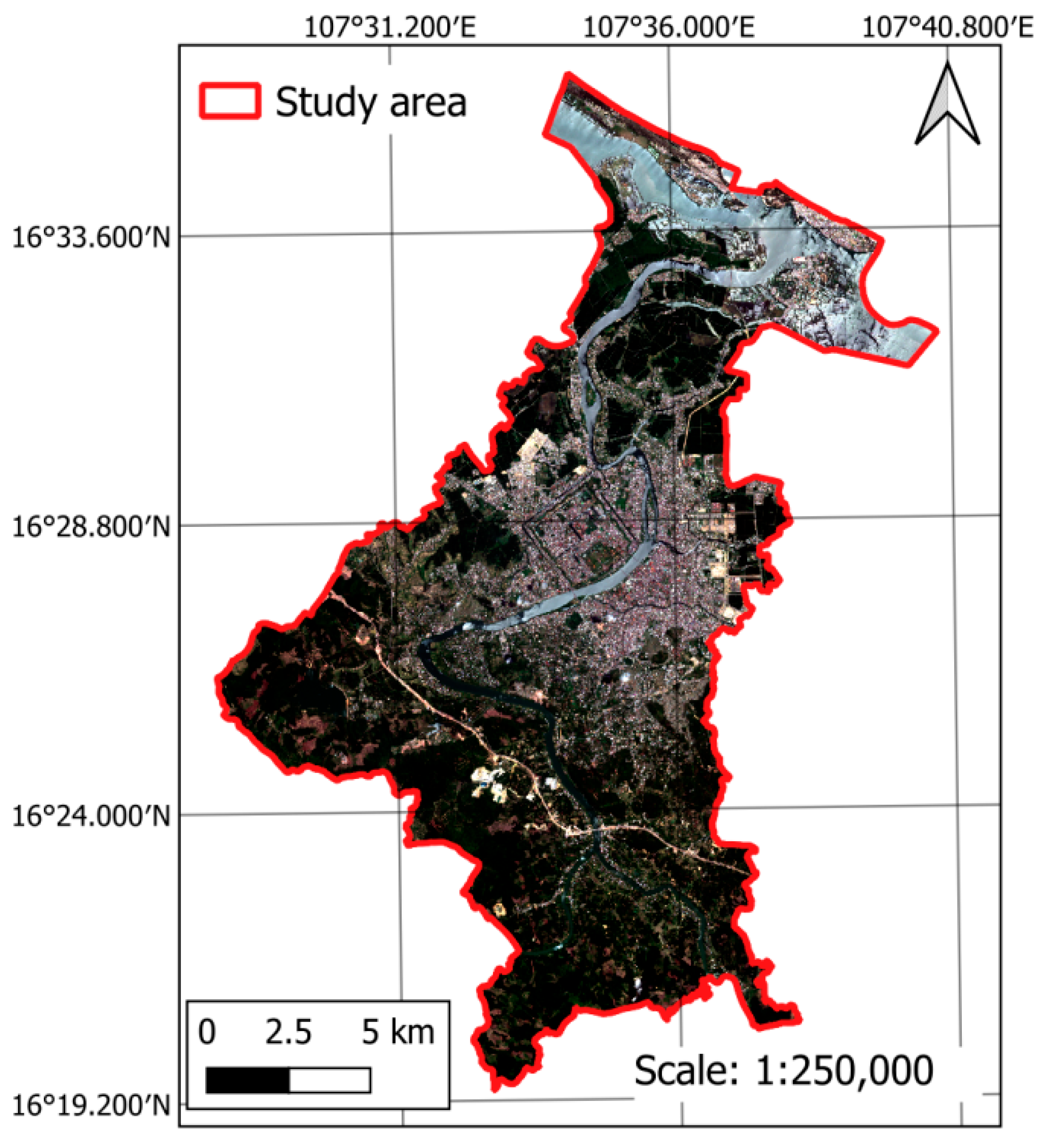
Hue City, situated along the Central Coast of Vietnam, is an administrative and cultural center of the region. Hue is internationally recognized as a UNESCO World Cultural Heritage city. The area encompasses the Complex of Hue Monuments—a renowned site of outstanding historical, architectural, and cultural value. The city’s urban center (refer to Figure 2), comprising Phu Xuan Ward and Thuan Hoa Ward, spans a total area of approximately 266 km2. This urban center is selected as the study area of the current work.
Geographically, Hue City lies in a low-lying coastal plain. Its border contains the Perfume River, with surrounding mountains and foothills. These geographical features shape the area’s climate conditions. The city experiences a tropical monsoon climate, characterized by distinctive wet and dry seasons. In recent years, the region has faced escalating climate challenges, particularly frequent and severe heatwaves and droughts attributed to global warming and urbanization. During the 2024 dry season, recorded temperatures in Hue rose beyond 42 °C for consecutive days, marking historic extremes and causing significant distress to both residents and tourists [36,37]. This fact necessitates comprehensive strategies to improve urban living conditions, especially for vulnerable communities in the urban core.
Addressing urban heat stress through the enhancement of blue-green spaces represents a sustainable and nature-based mitigation approach, especially vital during periods of intense heat waves. As heat extremes become more common in the city, it is crucial to quantitatively assess the CI of urban blue-green spaces; this assessment enables effective interventions that improve thermal comfort and public health. Hence, this study focuses on investigating spatial variations in blue-green space distribution within Hue City’s urban core, with emphasis on urban morphology and topographical characteristics.
To support geospatial modeling of LST and landscape analysis in Hue City, this research utilizes a collection of remote sensing datasets. Landsat 8 imagery, acquired between May and September 2024, provides LST measurements at a 30-m resolution. Sentinel-2 data, collected in 2024, is employed to construct a detailed land use and land cover (LULC) map. Additionally, elevation information is retrieved from the NASA SRTM Digital Elevation Model [64] at a 30-m scale. The used remote sensing datasets are summarized in Table 1.
LULC mapping in this study employs a machine learning-based classification workflow to ensure high accuracy. Sentinel-2 satellite imagery was processed and analyzed using a random forest (RF) classifier implemented within the Google Earth Engine (GEE) platform. Via several trial-and-error runs, the selected RF model consists of 30 trees, incorporating a total dataset of 2000 samples, with 500 samples assigned to each class. The LULC classes include bareland, built-up, vegetation, and waterbody. The dataset was divided into 70% for training and 30% for testing, resulting in a satisfactory testing accuracy of roughly 93%. The detailed classification performance is summarized in Table 2.
All Sentinel-2 image bands were standardized to a 10-m resolution within GEE. The nearest neighbor resampling is employed to upsample the bands with 20-m resolution (B5, B6, B7, B8A, B11, and B12) to ensure consistent spatial resolution for the data classification process. Subsequently, for CI mapping and prediction, all classified maps were further standardized to 30 × 30 m and processed using the QGIS (version 3.34.10).
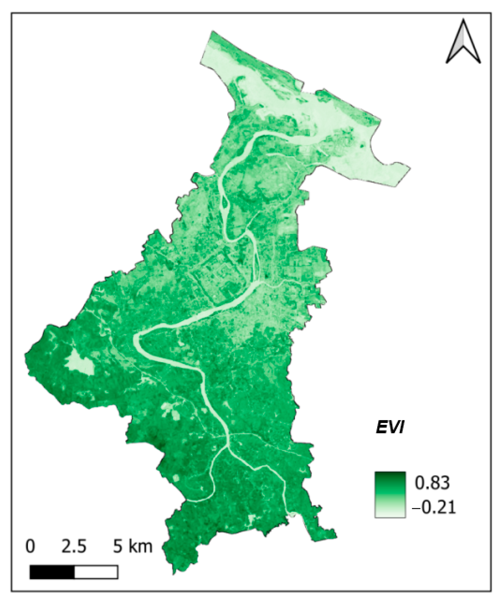
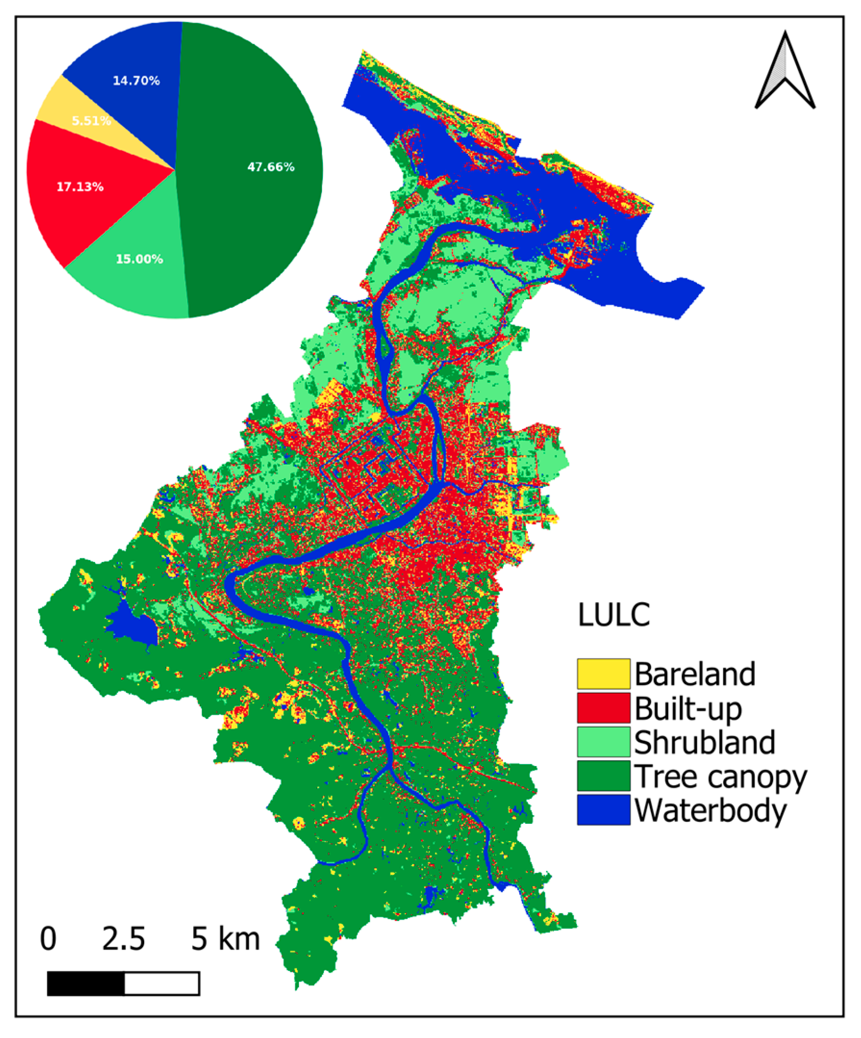
Vegetation was further categorized into shrubland and tree canopy types, guided by the enhanced vegetation index (EVI)’s threshold value—as recommended in [65]. Specifically, vegetated areas with EVI < 0.5 were categorized as shrubland, while those with EVI ≥ 0.5 were identified as tree canopy. This categorization allowed for precise mapping of urban green spaces, supporting correct evaluation of cooling effects in the study area. The EVI map and the resulting LULC map are presented in Figure 3 and Figure 4, respectively. The EVI, a widely used index for vegetation monitoring, is given by [66,67]:
E V I = G × ρ n i r ρ r e d ρ n i r + ( C 1 × ρ r e d C 2 × ρ b l u e ) + L
where L = 1 is a soil adjustment factor; C1 (6.0) and C2 (7.5) are the coefficients used to take into account the scattering of aerosol in the spectral bands; ρ n i r , ρ r e d , and ρ b l u e denote reflectance at the Near-Infrared, red, and blue wavelengths, respectively; G (2.5) denotes the gain factor.
It is acknowledged that there is a difference in acquisition periods between the Sentinel-2 and Landsat 8 datasets. This discrepancy may introduce certain temporal inconsistencies, particularly related to vegetation phenology. For Sentinel-2 imagery used in LULC and EVI mapping, the data collected throughout 2024 were employed to attain an annual composite that ensures consistent and cloud-free surface observations across the study area. This approach was necessary because parts of Hue City experience frequent and persistent cloud cover, even during the dry season. This fact often hinders clear observations of the land cover in the study area. By utilizing an annual composite, the study aims to produce the most up-to-date and representative mapping of land surface conditions.

2.2. Land Surface Temperature Retrieval

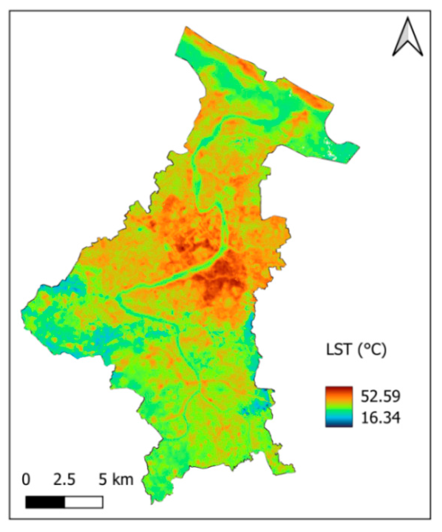
The thermal band from Landsat 8 imagery was utilized to extract LST data for the study area, focusing on records from the 2024 dry season, a period marked by multiple heat waves in the region. The resulting LST map, depicted in Figure 5, was prepared in QGIS. The preparation of this map includes several steps carried out in the GEE’s code editor.
Initially, spectral band values from Landsat 8 were converted to spectral radiance following the method described by [68]. Subsequently, to acquire the emissivity-corrected LST, land surface emissivity and the Normalized Difference Vegetation Index (NDVI) are computed [69,70]. The NDVI was computed using the 4th (red) and 5th (near-infrared) bands of Landsat 8 as follows:
N D V I = B 5 B 4 B 5 + B 4
where B4 and B5 represent band 4 (red) and band 5 (near-infrared), respectively.
The thermal band (B10) is extracted from the GEE’s data catalog. To transform the value of the thermal band into spectral radiance, the following equation is used [68,71]:
T B = M R F + B 10 × A R F
where B10 is the digital number of band 10; MRF (0.0003342) denotes the multiplicative rescaling factor; ARF (149) represents the additive rescaling factor.
Accordingly, the emissivity-corrected LST is given by [69]:
T S = T B 1 + ( λ × T B / ρ ) × ln ( ε ) 273.15
where TS denotes the estimated surface temperature measured in Celsius (°C); λ (10.8 µm) is the wavelength of emitted radiance; ρ = h × c / b (1.438 × 10⁻² mK), where h is Planck’s constant (6.626 × 10⁻³⁴ Js), c denotes the velocity of light (2.997 × 10⁸ m/s), and b denotes Bolzmann’s constant (1.38 × 10⁻²³ J/K); the factor of 273.15 is employed to convert the temperature from Kelvin (K) to Celsius (°C); the factor ε represents the land surface emissivity.
The land surface emissivity is calculated as follows [70]:
ε = 0.004 × P υ + 0.986
where P υ is the vegetation proportion computed in the following manner [68]:
P υ = ( N D V I N D V I min N D V I max N D V I min ) 2
where NDVI, NDVImin, and NDVImax are the values of NDVI, minimum NDVI, and maximum NDVI at a pixel in the map, respectively.

2.3. Cooling Intensity and Its Explanatory Variables

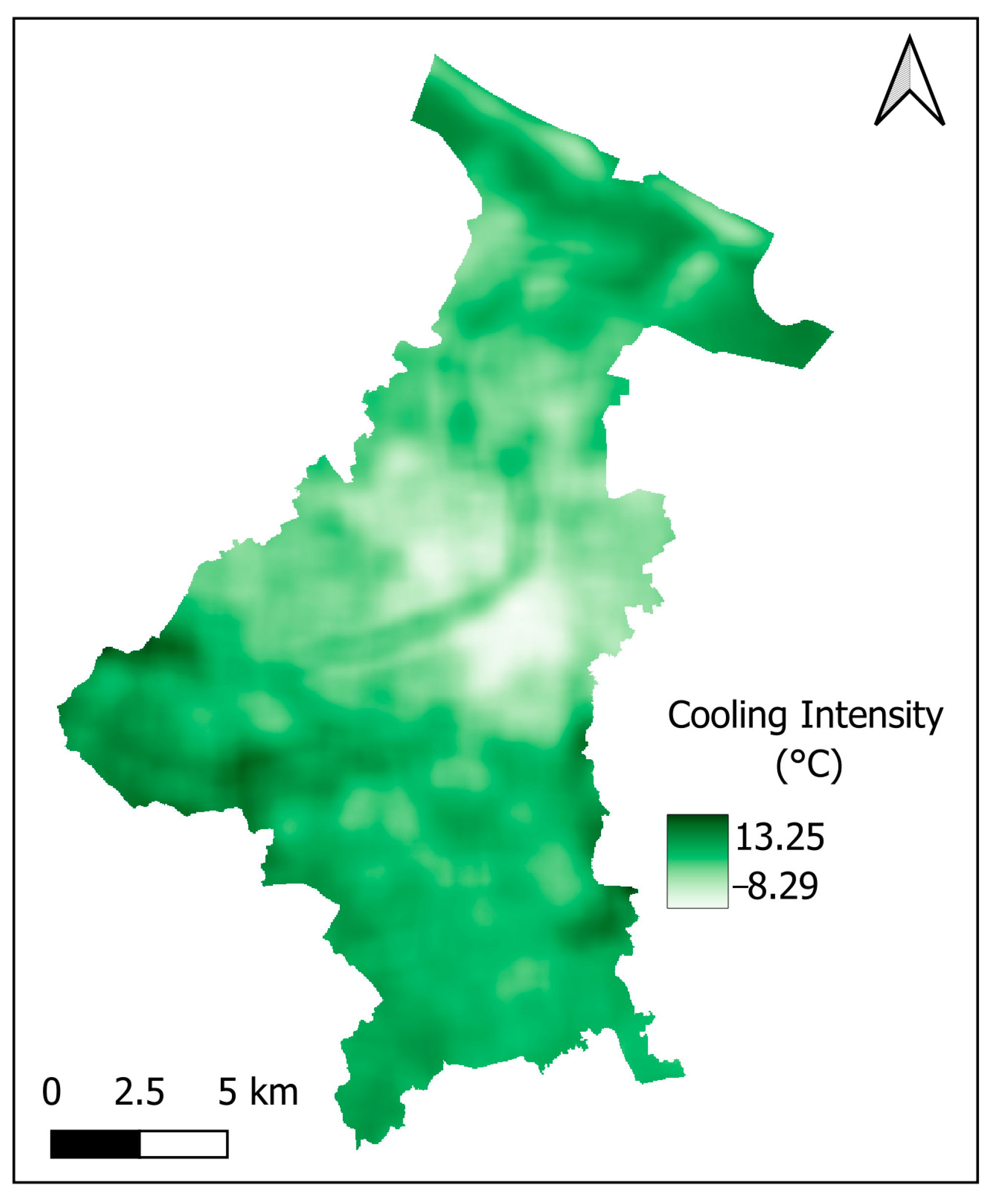
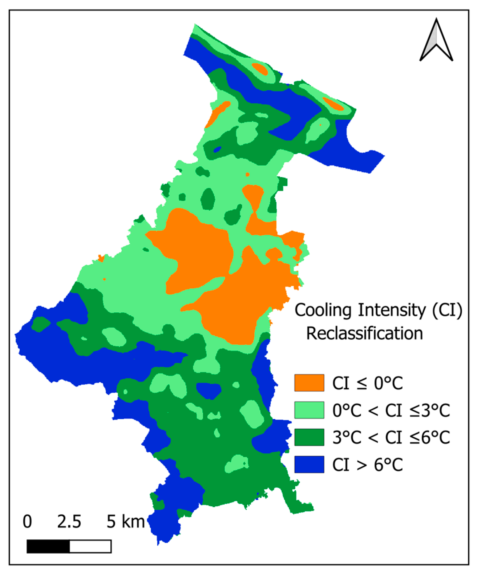
In this study, CI is employed as a quantitative measure to assess the thermal performance of urban blocks measuring 900 × 900 m (30 × 30 pixels) within the study area. The CI is calculated by subtracting the mean LST of an urban block from the mean LST of all built-up pixels across the study area. Based on the LST map analysis, the average LST of all built-up areas is found to be 40.28 °C. This approach enables the evaluation of each block’s relative effectiveness in mitigating urban heat, with higher CI values indicating greater reductions in urban LST compared to the region-wide built-up average. The CI map is presented in Figure 6.
In summary, the CI is calculated as follows:
C I = L S T m B u i l t u p L S T m B l o c k
where CI, L S T m B u i l t u p , and L S T m B l o c k denote the CI of a block, average LST of all built-up pixels, and the average LST of a block, respectively.
It is noted that to minimize the irregular influence of edge pixels on the analysis, a buffer zone of 1000 m is established around the study area’s boundary. The CI is calculated for all pixels located within this buffer zone; however, only data corresponding to pixels contained within the study area are selected for further analysis. This process is used to prevent unrealistic results that may arise from boundary effects and ensure an accurate assessment of CI across the urban landscape.
To model the spatial variation of CI, this study uses the following factors:
(i)
Topographical variables: average elevation, slope, aspect, topographic position index (TPI).
(ii)
Landscape composition: percentages of landscape (PLAND) of bareland, shrubland, tree canopy, and waterbody.
(iii)
Proximity features: average distance to coastline, river, road, shrubland, tree canopy, and waterbody.
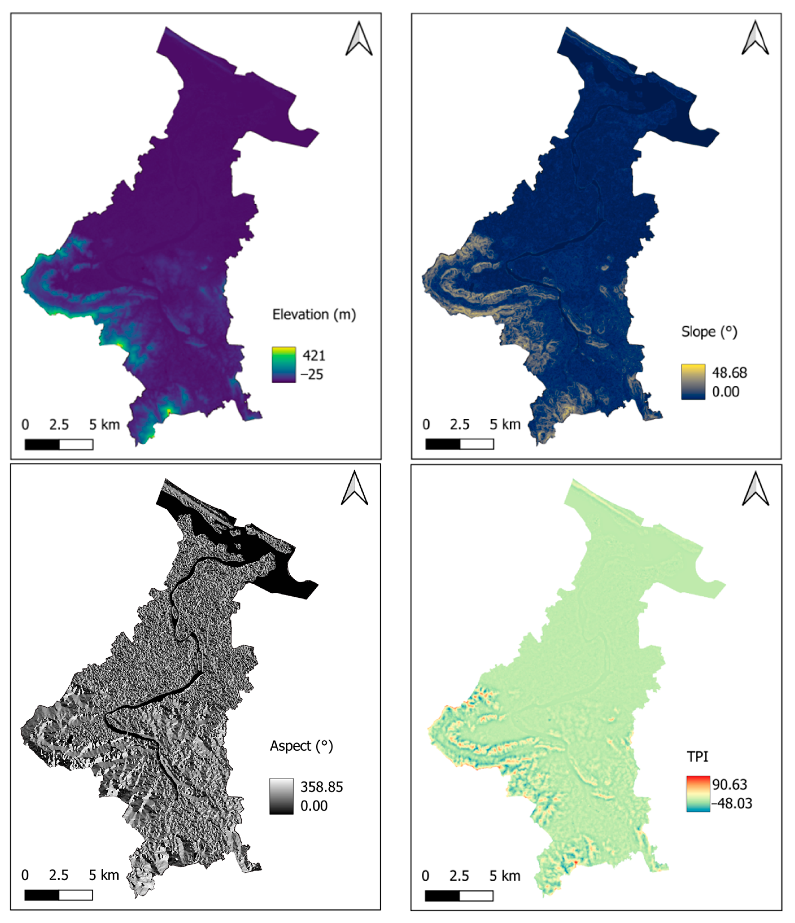
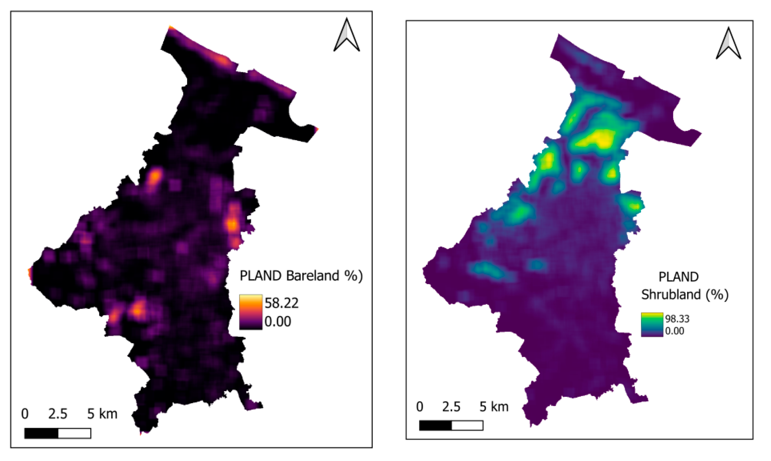
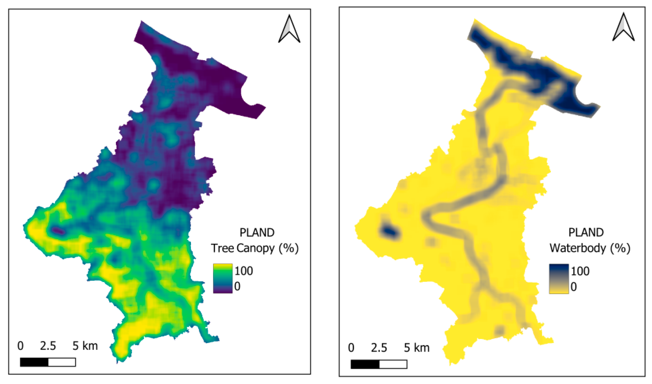
The aforementioned variables collectively capture the influence of both physical terrain and landscape configuration on the CI across urban blocks. Topographic variables have been shown to significantly influence the thermal behavior in urban environments [72,73]. The maps of topographic features are presented in Figure 7. Moreover, it is widely recognized that the primary driver of changes in urban LST is the conversion of natural and vegetated areas into impervious surfaces, such as concrete and asphalt [74]. Therefore, landscape composition or PLAND should be employed in the analysis of urban heat stress [24,75,76,77]. The PLAND maps are demonstrated in Figure 8. The landscape composition index can be computed as follows [78]:
P L A N D = i = 1 N a i A × 100 %
where ai is the area (m2) of the ith class of interest (e.g., tree canopy); A is the total area of the block (m2).
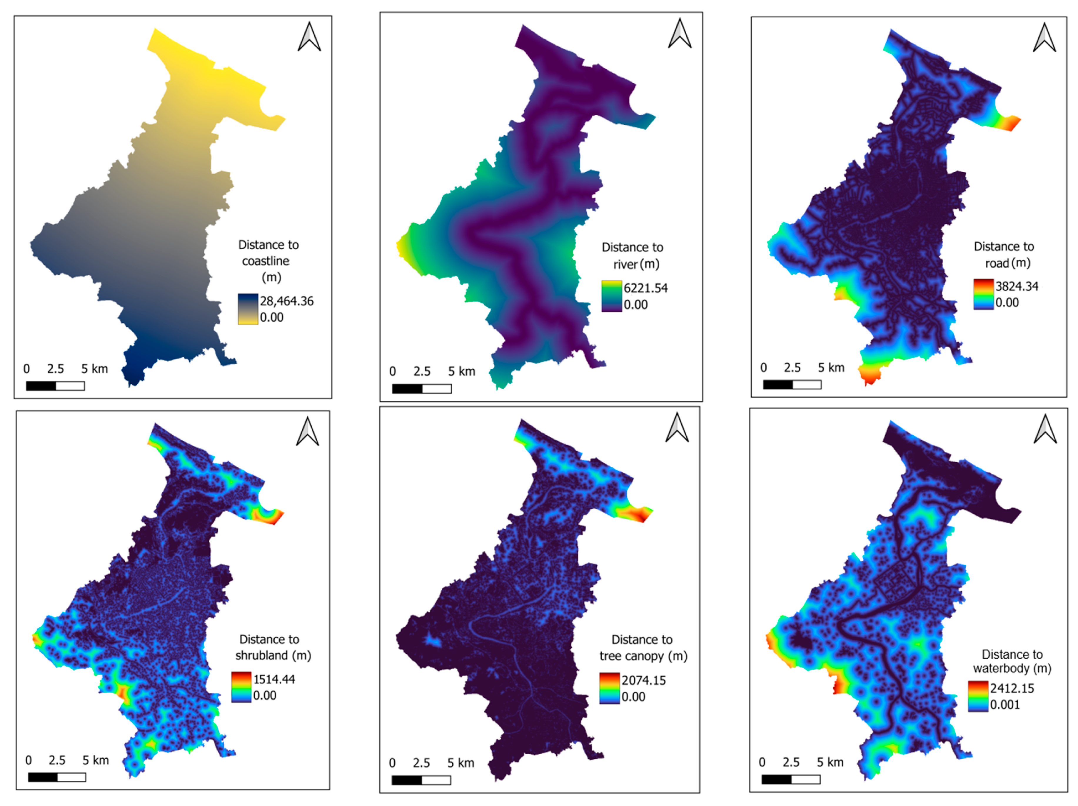
Proximity features, including the distance to coastline, river, road, shrubland, tree canopy, and waterbody, essentially influence the CI within urban blocks [79,80,81,82]. Urban blocks located closer to water bodies (coastlines, rivers, channels, and retention ponds) benefit from enhanced evaporative cooling and increased humidity, resulting in lower LST compared to those farther away. Tree canopy and shrubland patches also enhance CI of neighboring areas by providing shade and facilitating heat dissipation through transpiration, which reduces ambient temperature within and around the block. Conversely, blocks closer to roads and other impervious surfaces tend to experience higher LST compared to those surrounded by natural surfaces due to the absorption and retention of heat. In this study, the road data in Hue City is extracted from the OpenStreetMap source via https://extract.bbbike.org/ (accessed on 7 January 2025). The maps of proximity features are shown in Figure 9.

2.4. Extreme Gradient Boosting Machine for Nonlinear Function Approximation

Extreme gradient boosting machine (XGBoost) [83] a popular machine learning framework based on gradient-boosted decision trees. This method is widely recognized for its efficiency, speed, and outstanding performance in nonlinear data modeling [84,85]. For nonlinear function approximation, XGBoost builds a series of regression trees where each new tree aims to correct the residual errors of prior trees. This process results in highly accurate predictions.
XGBoost also incorporates regularization and pruning techniques that enhance model generalization. Therefore, the constructed model is less likely to suffer from overfitting and can achieve robust performance. For interpretability, combining XGBoost with Tree SHAP allows users to precisely quantify each feature’s influence on individual predictions [86,87]; this integration helps transform the model from a black box into a transparent system that provides insights to support decision-making processes.
To mitigate overfitting, XGBoost incorporates regularization parameters during model training that effectively constrain model complexity and restrict the risk of overfitting. This advanced approach enables XGBoost to accurately model complex, multivariate relationships while maintaining strong generalization to new data. As a result, not only are XGBoost-based models precise, but they are also robust against overfitting and capable of delivering reliable performance even when working with noisy datasets. To train the XGBoost model, the following loss function is used:
f o b j = i L ( y i , F ( x i ) ) + t Ω ( f t )
where Ω ( f ) = γ T + 1 2 λ j T w j 2 denotes a regularization term; T is the number of leaves employed in a tree f; w represents the score of a leaf j of f; γ is a threshold of the score function improvement used for tree splitting.
Furthermore, the Squared Error Loss (SEL) is often employed in nonlinear function approximation; its equation is given by:
L ( t , y ) = ( t y ) 2
where t and y are the actual and predicted dependent variables.
New decision trees are sequentially included in the overall model to minimize the following objective function:
f o b j t = i L ( y i , F t 1 ( x i ) + f t ( x i ) ) + t Ω ( f t )
Based on Taylor’s second-order approximation, the aforementioned objective function can be optimized and the score w j * of leaf j in a decision tree can be acquired as follows [88]:
w j * = i I j g i i I j h i + λ
where gi and hi denote the first and second order gradients of the loss function, respectively; I j is the data samples that are handled at leaf j.
The final XGBoost model can be expressed as follows:
F X G B o o s t = t = 1 M f t ( x )
where M denotes the number of individual decision trees.

2.5. Shapley Additive exPlanations (SHAP)

Shapley Additive exPlanations (SHAP) [89] is a powerful framework for interpreting machine learning models by attributing the contribution of each input feature to individual predictions. SHAP is founded upon principles from cooperative game theory. This method is used to compute Shapley values, which quantify how much each feature influences a model’s prediction for every instance. These values can also be used to infer the impact of variables on overall predictions. Therefore, SHAP facilitates transparency of the model’s structure and provides insights into its behavior.
Moreover, SHAP can be utilized to construct partial dependence plots, which visualize the average effect of a feature on model output. These plots display the average predicted effect of varying a single feature while keeping all other features constant. These plots support the understanding of the nature and strength of the relationship between a particular explanatory variable and the model’s output. Observing the partial dependence plots, users can acquire knowledge about the pairwise relationship between the influencing factor and the target output. One advantage of SHAP is the formulation of Tree SHAP, which is specifically designed for tree-based machine learning models. Tree SHAP stands out for its computational efficiency, as it leverages the structure of decision trees to rapidly compute exact Shapley values for individual predictions in tree-based models like XGBoost. This fact makes Tree SHAP highly practical for large datasets.

2.6. Metrics for Model Performance Evaluation

To assess how well the XGBoost predicts the CI, this study employs the Root Mean Square Error (RMSE), Mean Absolute Error (MAE), and coefficient of determination (R2) as evaluation metrics. RMSE indicates the average magnitude of prediction errors; this index is influenced by large errors. An RMSE closer to 0 implies more accurate predictions. MAE computes the average absolute difference between predicted and actual values. R2 measures the proportion of variance in the observed data explained by the model. R2 ranges from 0 to 1, where values closer to 1 reflect a better model. The aforementioned indices are calculated as follows:
R M S E = 1 N i = 1 N ( y i t i ) 2
M A E = 1 N i = 1 N | y i t i |
R 2 = 1 i = 1 N ( t i y i ) 2 i = 1 N ( t i t ¯ ) 2
where ti and yi denote the actual and estimated CI values of the ith sample, respectively; N represents the total number of samples; and t ¯ is the average value of the actual CI.

3. Cooling Intensity Predicting Results

3.1. Prediction Performance

Since XGBoost is a supervised learning approach, to predict the CI in Hue City, a GIS dataset including 30,000 data points is prepared. The statistical description of the dataset is summarized in Table 3. These data points are randomly sampled across the study area. A set of fourteen explanatory variables is used. The predictor variables take into account topographical features (average elevation, slope, aspect, and TPI), landscape composition (percentages of bareland, shrubland, tree canopy, and waterbody), and proximity metrics (average distances to coastline, river, road, shrubland, tree canopy, and waterbody). The dependent variable is the CI, which represents the magnitude of temperature reduction attributed to blue-green space landscape and other factors.
The dataset is randomly partitioned into a training set (70%) and a testing set (30%). The first set is used for model construction; the second set is reserved for testing the model’s generalization capability. It is noted that appropriate hyper-parameter setting is important to avoid an overfitted XGBoost model. Overfitting typically occurs when the model learns patterns specific to the training data, including noise or random variations. However, this model cannot generalize well to unseen samples. For the current dataset, an overfitted XGBoost model could predict CI accurately for the training data but perform poorly on the testing data. To mitigate overfitting, the hyper-parameters of the XGBoost model, including the number of trees, maximum tree depth, learning rate, L2-regularization coefficient, and L1-regularization coefficient, were carefully tuned via trial-and-error runs with the training dataset. Herein, the training dataset is randomly divided into two subsets: subset 1 (70%) and subset 2 (30%). The former is used to construct the model, and the latter is employed to evaluate its prediction performance. The experiment with these two subsets was conducted using various combinations of the model’s hyper-parameters to assess their suitability for the collected dataset.
Based on the aforementioned process, the hyper-parameters of XGBoost (the number of trees = 150, the maximum tree depth = 4, the learning rate = 0.2, the L2-regularization coefficient = 0.01, and the L1-regularization coefficient = 0.001) are selected. Overall, this section aims to construct a data-driven framework that delivers an accurate assessment of how landscape and topographical features influence spatial variations of CI.
The prediction performance of XGBoost is summarized by the scatter plots in Figure 10. Each data point in the plots represents a particular observation, with the x-axis corresponding to the actual CI and the y-axis to the predicted value. The red dashed line denotes the line of best fit; this line implies the ideal cases where the predicted CI perfectly matches its actual value. The points clustering closely around this line indicate highly accurate predictions. The larger the deviation from the line of best fit, the greater the prediction error.
In both the training and testing phases, the model achieves robust performance. The RSME values (0.49 in the training and 0.55 in the testing phase) indicate low deviations between the predicted and actual CI values. The MAEs, 0.37 for the training set and 0.41 for the testing set, imply that the range of the average prediction error is small across the data samples. As shown in the R2 values, the model is capable of explaining 98% of the variance in CI for the training data and 97% of that for the testing data. This fact confirms that the model maintains very high explanatory power and continues to capture a high portion of the variability in CI. The balance between the performances in the two phases demonstrates that the model generalizes well to unseen data and does not suffer from overfitting.
The XGBoost is then used to construct the maps that provide a detailed visualization of predicted CI and the corresponding prediction error across the study area. Figure 11a illustrates the spatial distribution of CI, which ranges from −8.22 °C to 13.46 °C. This fact, coupled with the robust prediction performance reported in Figure 10, highlights the model’s ability to capture the variation of cooling effect influenced by heterogeneous landscape features and microclimate conditions in the region. Figure 11b presents the prediction error, depicting regions where the model predictions deviate from observed values. As can be seen in the map, most areas exhibit low errors, while only a few localized patches display higher deviations. The prediction error ranges from −3.27 °C to 4.20 °C.
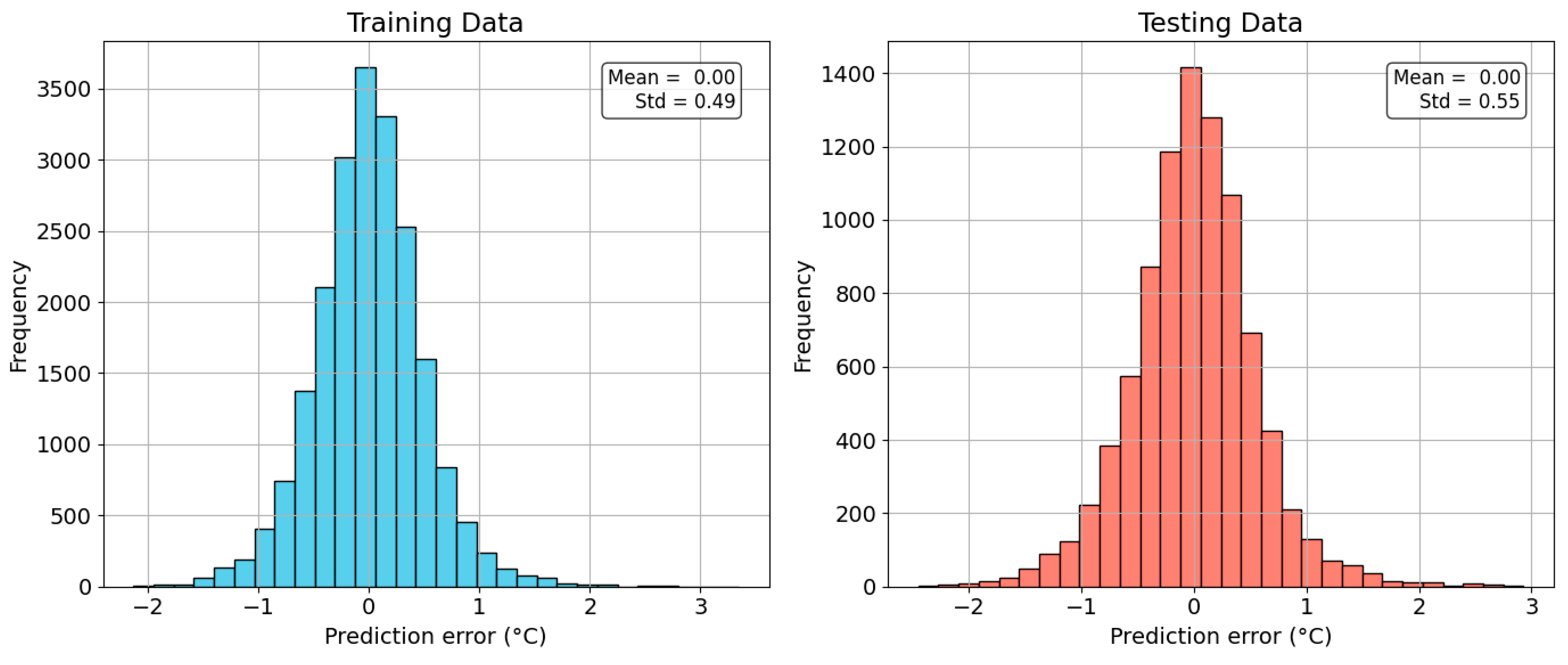
The histograms in Figure 12 reveal that the prediction error distributions for both training and testing data are highly symmetric and centered on zero. This fact indicates an absence of systematic bias in the XGBoost model’s predictions. For the training data, the mean prediction error is roughly zero and the standard deviation is 0.49 °C; these results show that most errors are small and tightly clustered around the mean. The histogram for the testing data shows a similar pattern, with a mean close to zero and a slightly higher standard deviation of 0.55 °C, reflecting a small increase in error dispersion when the model is used to predict unseen data. In general, the majority of prediction errors fall within the range of values between −2 °C and 2 °C. This suggests that extreme prediction errors, located in the two tails, are rare and that the model reliably yields accurate estimates of CI in the study area.
Moreover, this analysis uses regression error characteristic curves (REC) [90] to evaluate the difference between measured and XGBoost-predicted cooling intensities. The REC curves for the XGBoost model, shown in Figure 13, provide a detailed visualization of how well the model predicts CI on both the training and testing sets. These curves plot the absolute prediction error (x-axis) against the percentage of samples predicted with an error below that threshold (y-axis). In more detail, the REC curve presents the fraction of data samples for which the absolute deviation between observed and predicted cooling intensities falls within a given error threshold. The further left and higher the curve, the better the model’s predictive performance. It is because a larger proportion of samples are associated with smaller errors. By further inspecting the REC curves, it can be seen that for the training set, 90% of predictions have an absolute error below 0.81 °C, and 95% are lower than 1.01 °C. For the testing set, 90% of predictions have an absolute error less than 0.89 °C, and 95% are lower than 1.15 °C. These thresholds clearly show the model’s reliability in CI estimation.
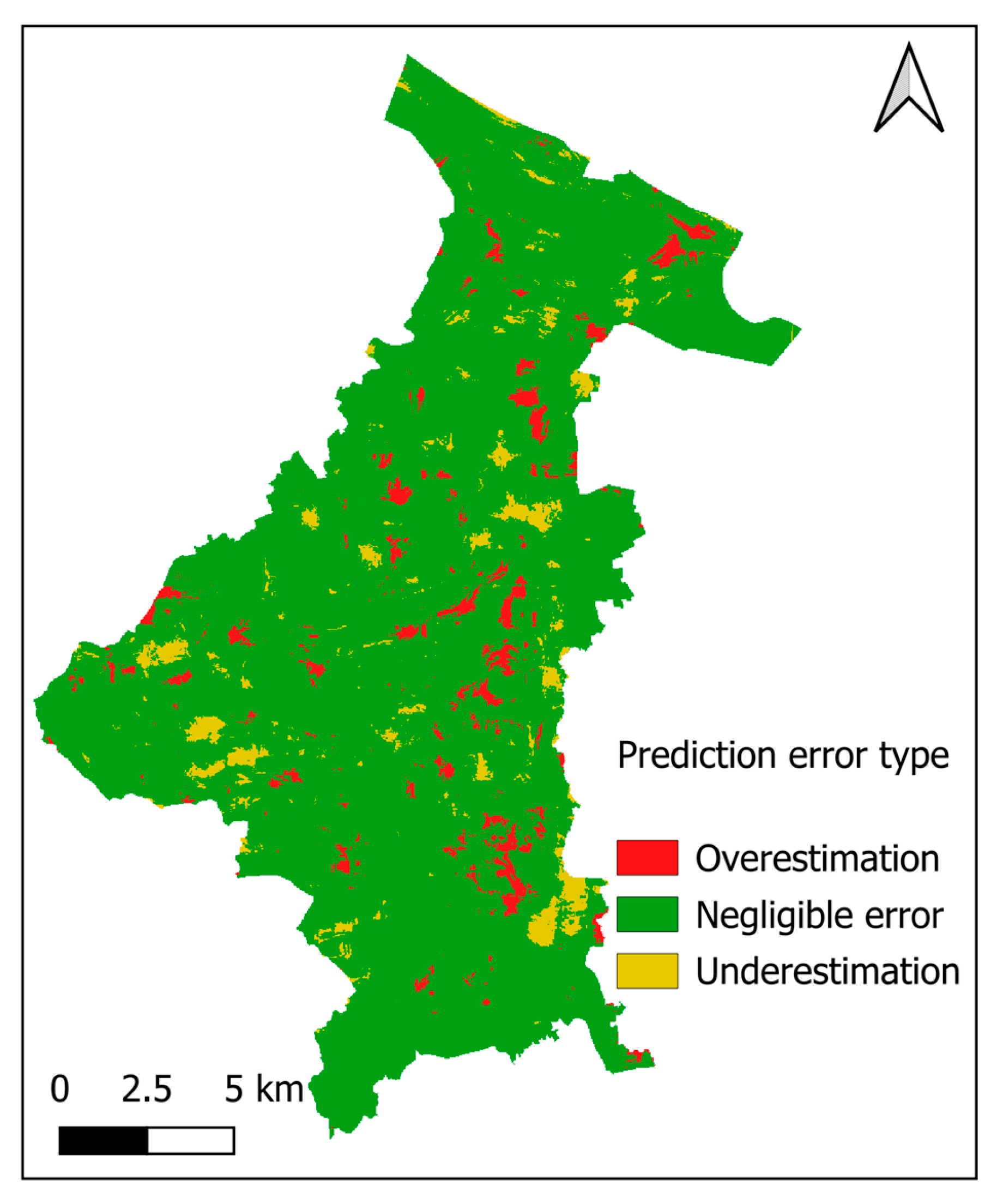
The map of prediction error types (Figure 14) visually categorizes the spatial distribution of errors or residuals—where the error is defined as the actual CI minus the predicted intensity—into three groups: overestimation, underestimation, and negligible error. In this context, errors within the interval [−1, 1] reflect negligible error (green areas), where the predicted values closely match actual measurements. Moreover, a negative error (error < −1) means the predicted CI exceeds the actual value, representing overestimation (red areas). Conversely, a positive error greater than 1 (error > 1) indicates the actual CI is much higher than the predicted value, corresponding to underestimation (yellow areas).
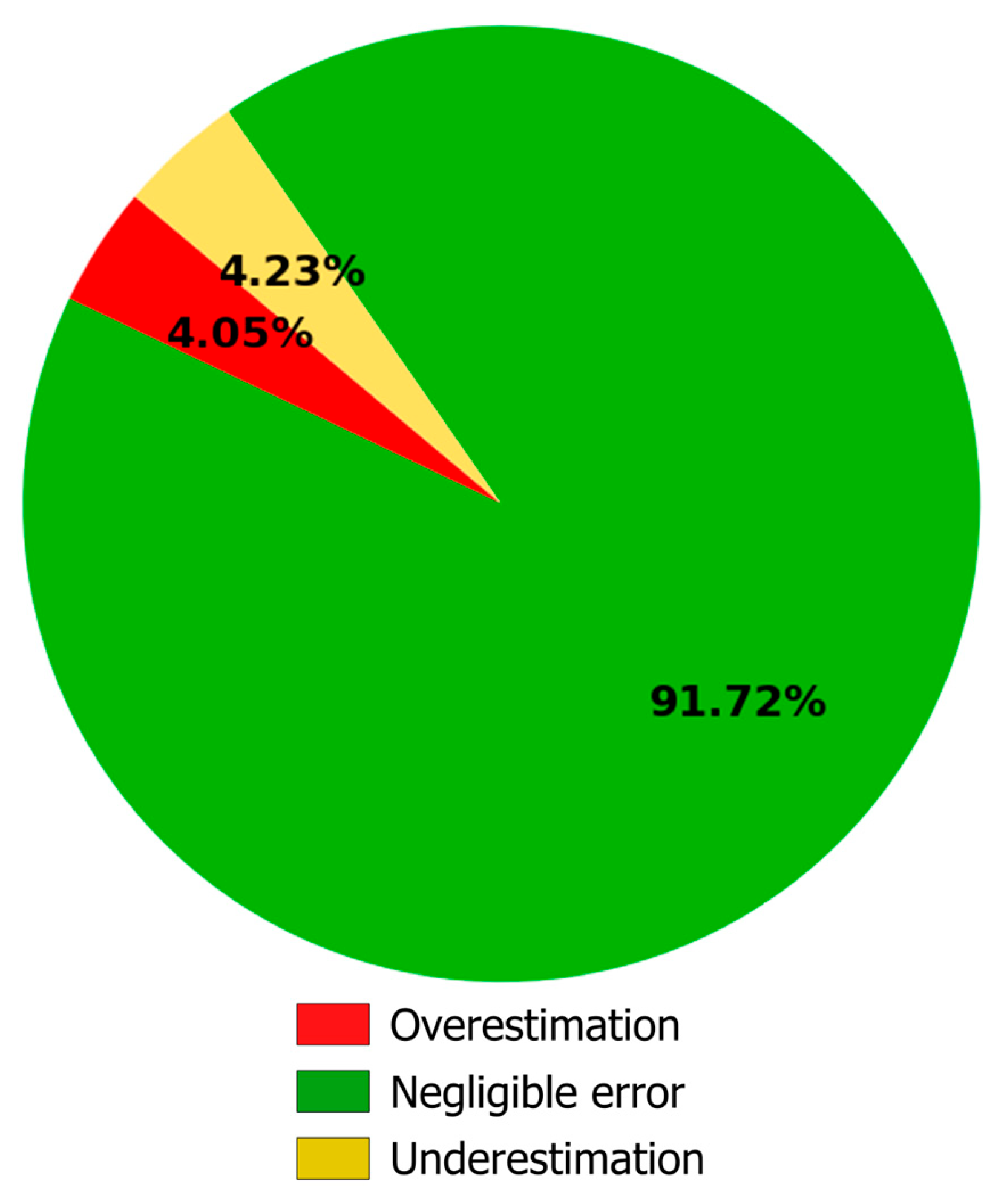
For CI estimation, underestimation is generally more desirable than overestimation. This is because overestimating cooling potential might lead urban planners to expect greater thermal comfort than what can actually be delivered. Overestimation can negatively impact planning and mitigation strategies. In contrast, underestimation tends to facilitate conservative planning, ensuring that anticipated benefits are at least met or exceeded. The pie chart (Figure 15) shows that negligible errors dominate, accounting for 91.72% of all predictions, while underestimations and overestimations make up only 4.23% and 4.05%, respectively. This distribution highlights the high overall accuracy of the model, with only a small risk of misleading overestimates and an even smaller tendency toward cautious underestimation. The outcomes demonstrate that XGBoost is highly suited for the task at hand.

3.2. SHapley Additive exPlanations (SHAP)

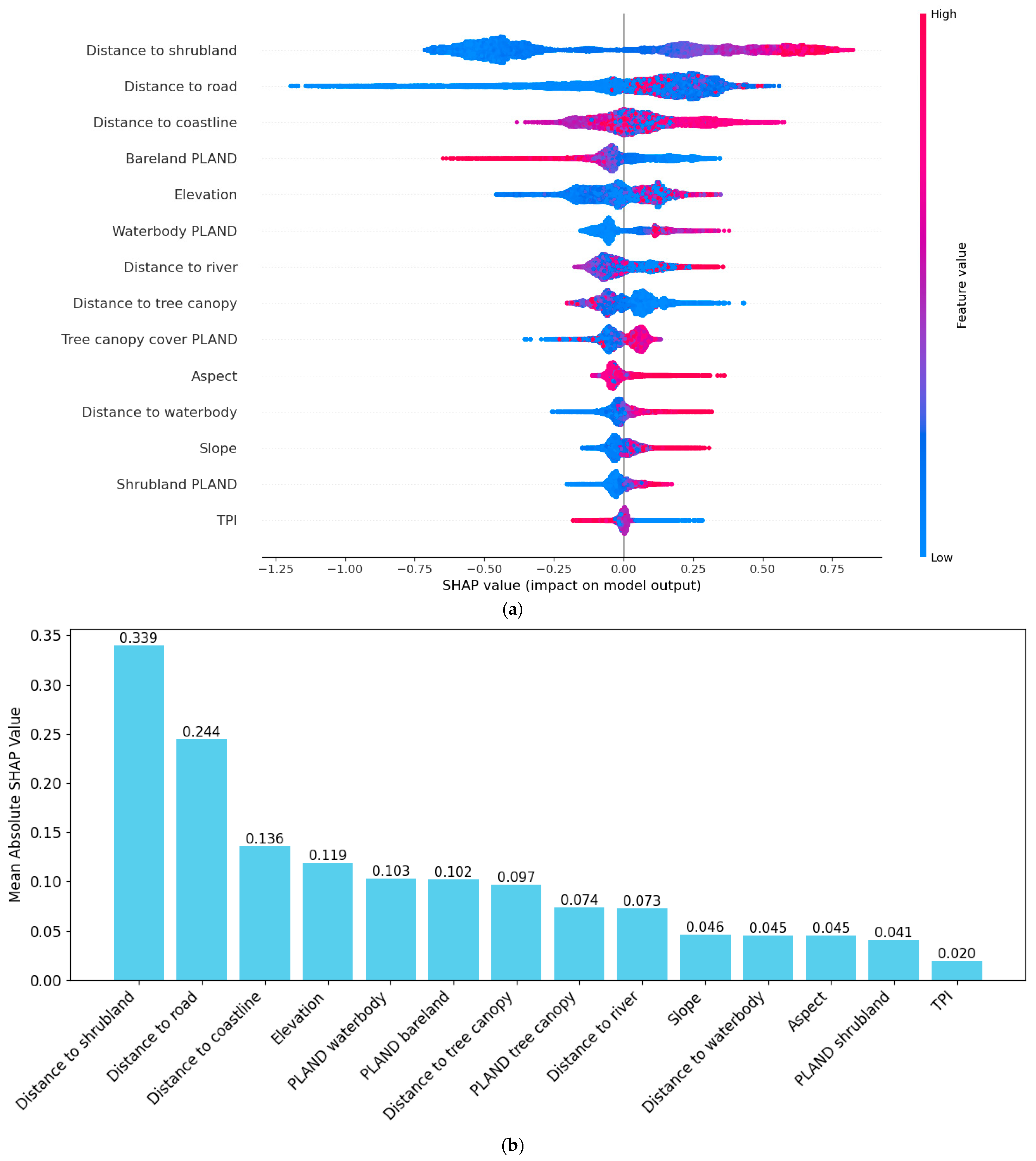
In this study, the SHAP framework is integrated with XGBoost to investigate the drivers behind the model’s results. By employing Tree SHAP, the analysis supports clear interpretation of both the ranking and directional influence of each input feature on CI predictions across the study area. This method enhances the transparency and interpretability of the modeling process. The result is summarized by the SHAP’s analyses in Figure 16.
According to the SHAP’s impact plot in Figure 16a, distance to shrubland is the most influential variable. Distance to road and distance to coastline also rank highly. For distance to road, proximity tends to enhance predicted cooling. However, for distance to coastline, the relationship between this factor and CI in Hue City is complex, although certain areas closer to the beach do show some degree of enhanced CI. Bareland PLAND is the highest among the PLAND indices; it achieves the fourth rank. Waterbody PLAND and tree canopy cover PLAND also contribute considerably to the model but have less influence than that of distance to shrubland, distance to road, and distance to coastline. Meanwhile, shrubland PLAND is the least impactful variable in the group of PLAND indices; this fact indicates its relatively minor effect on cooling prediction. Besides elevation, the other topographical factors (i.e., aspect, slope, and TPI) generally attain lower rankings, reflecting their comparatively weaker impact on CI outcomes for the study area.
Moreover, Figure 16b presents the mean absolute SHAP value for each feature. This metric quantifies the average contribution of every variable to the model’s prediction of CI. The mean absolute SHAP value indicates the average influence of a feature on the XGBoost’s prediction—regardless of whether the effect is positive or negative. It is noted that the SHAP impact plot in Figure 16a displays the overall distribution and directionality of SHAP values for each feature across the dataset. Meanwhile, Figure 16b presents a magnitude-based summary by computing each feature’s overall impact on the model as a single mean absolute SHAP value. Notably, there is a slight difference in feature ranking between the two plots. This discrepancy arises because the impact plot incorporates both variability and directionality in the feature effects, while the mean absolute SHAP value only reflects the overall average impact magnitude. However, both plots consistently highlight variables such as distance to shrubland, distance to road, and distance to coastline as key predictors driving the model’s estimations of CI in the study area.
Inspecting the direction of the influence, it can be seen that for distance to shrubland, low values (closer proximity) are strongly associated with negative SHAP values, meaning that being near shrubland significantly reduces the predicted CI. The same fact holds true for the factor of distance to road. This fact is understandable because areas closer to roads are often subject to higher levels of anthropogenic heat. Moreover, based on SHAP, it can be seen that shrubland in the study area does not provide a cooling effect; in fact, areas closer to shrubland are associated with a reduction in predicted CI. In contrast, tree canopy exhibits a clear cooling effect, as areas closer to tree canopy cover are associated with higher predicted CI. Regarding landscape composition, a smaller proportion of bareland PLAND is associated with higher CI. In contrast, greater values of waterbody PLAND, tree canopy cover PLAND, and shrubland PLAND correspond to enhanced CI.
Moreover, partial dependency analysis is conducted with landscape composition variables regarding blue-green spaces. The partial dependency plots derived from SHAP are presented in Figure 17. This graph provides information about how specific landscape composition variables influence CI while accounting for interactions with other features. The partial dependency analysis helps visualize the marginal effect of each variable, allowing for recognition of suitable ranges of variables in landscape planning and management. The results of the partial dependency analysis reveal that CI generally increases with the proportion of the blue-green spaces in Hue City.

4. Discussion

4.1. Prediction Performance of the Machine Learning Framework

This study presents an innovative framework that integrates geospatial data analysis and interpretable machine learning for modeling CI in Hue City, Vietnam. For relationship modeling, XGBoost is employed to establish a robust functional mapping between CI and its explanatory variables—addressing the inherent nonlinearity and multivariate nature of the GIS dataset. XGBoost demonstrates satisfactory performance; this method is capable of explaining 98% of the variance in CI for the training data and 97% for the testing data. This high predictive accuracy confirms XGBoost’s strength in handling complex, non-linear relationships and interactions among diverse geospatial input features. The sophisticated gradient boosting algorithm iteratively improves model performance by focusing on residual errors, making XGBoost highly effective in predicting outcomes in large-scale and nonlinear datasets. Furthermore, the model’s regularization techniques also help prevent overfitting, thereby supporting robust generalization to unseen samples. Accordingly, this machine learning approach is recommended for geospatial modeling of CI in other regions.

4.2. Cooling Intensity (CI) in Hue’s Urban Center

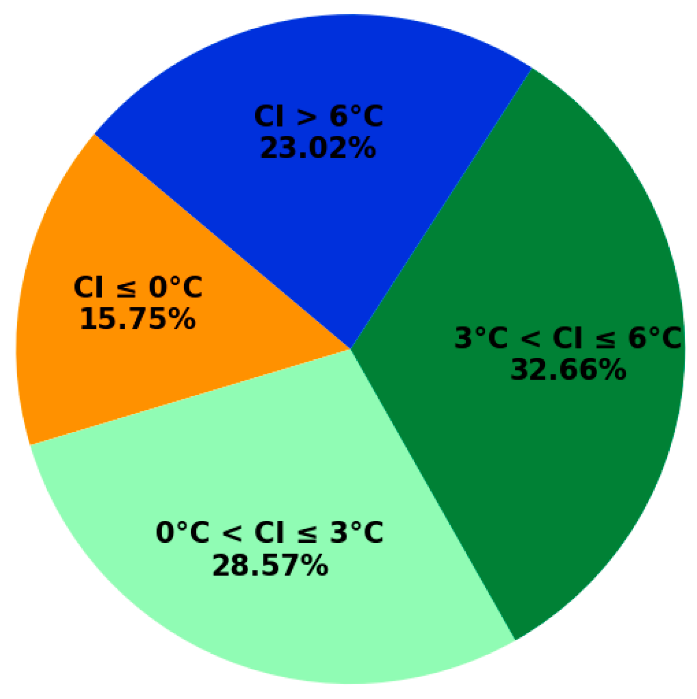
The proportion of area classified by CI across the study area is demonstrated in Figure 18. The largest segment corresponds to regions with moderate CI, where 3 °C < CI ≤ 6 °C, consisting of 32.66% of the total area. Areas experiencing mild cooling performance (0 °C < CI ≤ 3 °C) account for 28.57%, while zones with high cooling performance (CI > 6 °C) occupy 23.02% of the study area. The smallest proportion (CI ≤ 0 °C), which corresponds to negative cooling, covers only 15.75% of the area. These results suggest that a significant majority of the study area benefits from moderate to high cooling effects.
Figure 19 demonstrates the spatial distribution of CI classes across the study area. As a World Cultural Heritage site, Hue City is characterized by its preservation of blue-green infrastructure, including water bodies, parks, shrubland, and tree canopy coverage. These features are strategically intermingled throughout the urban environment, resulting in extensive areas characterized by moderate to high CI. However, 15.75% of the area still experiences negative CI. These zones, primarily situated within the dense urban areas, are most severely impacted during heat waves. This fact is largely due to the high concentration of impervious surfaces, reduced vegetation cover, and intense anthropogenic activity—conditions that intensify the UHI effect and negate the capacity of natural cooling. Consequently, interventions are urgently needed in these hotspots to alleviate thermal discomfort and enhance public health in the city, especially during extreme heat events.

4.3. Urban Planning Implications for Enhancing Blue-Green Space’s Cooling Intensity

Effective urban planning is critical for optimizing CI and mitigating urban heat stress in Hue City—a rapidly urbanizing region. Based on SHAP analysis, urban development should prioritize interventions that minimize bareland in the study area. The reason is that bareland PLAND shows a negative association—a higher bareland proportion diminishes CI. This fact implies that local authorities should prevent bareland expansion and replace this LULC type with vegetation and water surface.
Furthermore, dense shrubland within the study area should also be limited. Converting shrubland to tree canopy, retention ponds, and drainage channels is strongly recommended. It is because tree canopy cover and waterbody presence exhibit clear positive effects on CI. Based on partial dependence analysis, planning efforts should focus on increasing the proportion of tree canopy and enhancing waterbody coverage.
Via visual interpretation of the partial dependence plots, the ranges for tree canopy PLAND (30–80%) and waterbody PLAND (10–40%) are associated with the most pronounced increases in CI. Therefore, these ranges of urban blue-green spaces are recommended for achieving the most desired CI in the study area. Moreover, expanding existing blue-green space coverage and enhancing public accessibility to water bodies or urban parks are crucial for improving cooling benefits in cities [91]. This is because the tree canopy and water bodies can have an impactful cooling effect on adjacent areas. Budzik et al. [24] pointed out that blue-green spaces adjacent to dense urban areas are capable of cooling the neighboring region up to 393 m further and by 10 °C.
SHAP analysis reveals that waterbody PLAND exerts a greater impact on CI than tree canopy PLAND. This finding suggests that increasing the proportion of water bodies can deliver stronger cooling effects compared to expanding tree canopy coverage. These results emphasize the importance of prioritizing blue infrastructure within the study area. This approach aligns with findings from [53], which showed that water bodies not only deliver stronger CI but also have much wider cooling ranges compared to tree-based green spaces.
It is noted that although urban blocks with a higher overall proportion of shrubland (PLAND) are associated with higher CI, areas closer to this type of land cover tend to have lower CI. This fact might arise from its spatial context in the study area. It is because shrubland is commonly located adjacent to roads, bareland, and construction sites, which are associated with higher surface temperatures and anthropogenic heat. In contrast, urban blocks with a higher overall proportion of shrubland generally include more interspersed green spaces or less developed surroundings, which can contribute to improved cooling capacity. This fact highlights the need to consider both spatial distribution and characteristics of neighboring LULC when considering the cooling effects of urban green spaces in Hue City.
Additionally, in developing new urban districts in Hue City, it is recommended to allocate a designated proportion of land for blue-green spaces—such as reserving 30% for tree canopy and 10% for water bodies—to create ecologically beneficial landscapes within these communities. Furthermore, urban greening can be substantially increased by utilizing building rooftops, walls, and other underused spaces for vegetation, thereby expanding the overall green spaces without compromising built-up areas [92]. Methods such as rooftop gardens on commercial buildings not only enhance the aesthetic aspect but also contribute valuable green cover to the city. Moreover, maintaining urban parks and forested corridors plays a vital role in mitigating the UHI effect through shade provision, evaporative cooling, and lowering surface temperatures, which collectively reduce the demand for artificial cooling and improve urban sustainability [55].
The research findings can be extended beyond Hue City and offer practical implications for neighboring cities in Vietnam that are aiming to mitigate urban heat stress through effective blue-green infrastructure planning. The data-driven SHAP-based framework enables city planners to prioritize interventions by identifying which landscape and proximity features most strongly influence local CI. Since the proposed approach is data-driven, it can be readily adapted to other urban regions with different climatic and spatial contexts when suitable local data is provided. For rapidly urbanizing cities facing land scarcity and increasing extreme heat events, the recommended strategies—such as minimizing bareland, optimizing proportions of tree canopy and water bodies, as well as integrating green infrastructure into the urban fabric—are widely applicable. Furthermore, the transferability of the proposed data-driven framework is reinforced by its grounding in remote sensing and machine learning. These approaches are accessible to many cities worldwide.

4.4. Research Limitations and Future Works

While this study incorporates various factors influencing CI, it is recognizable that the current set of variables may not fully capture the complexity of the task at hand. Other factors—such as building height, sky view factor, impervious surface fraction, spatial connectivity of blue-green spaces, and landscape shape indices—can also significantly influence CI but were not considered in this study. The absence of these variables may limit the model’s ability to take into account localized thermal dynamics, especially in areas with significant vertical variation, varying degrees of building density, and highly heterogeneous built environments.
While this study categorizes vegetation into shrubland and tree canopy types using EVI thresholds, it is acknowledged that this classification may not fully capture the diversity within small-scale green patches. The shrubland class may encompass mixed vegetation types that can differ in density, height, and moisture content, which may influence their cooling performance. Some shrubs may act similarly to low tree canopies with considerable cooling effects, while sparse or dry shrubland may provide limited or ineffective cooling effects under high humidity conditions.
Moreover, the accuracy of CI estimates in the study area may be compromised by the use of LST samples collected at different timestamps during the period from 1 May 2024 to 30 September 2024. Additionally, the presence of cloud-affected Landsat scenes can degrade data quality. Under these circumstances, the computed CI values might not accurately reflect true cooling effects in certain areas in Hue City. It is also recognized that the EVI threshold used to classify vegetation into shrubland and tree canopy may oversimplify the diversity of vegetation structures in tropical urban landscapes.
Another limitation lies in the use of Landsat 8 satellite data. While its 30 m spatial resolution offers a balance between spatial coverage and data acquisition frequency, it remains insufficient for effectively capturing fine-scale heterogeneity in vegetation and surface temperature within dense urban settings. This pixel size may merge small or fragmented features—such as narrow streets, isolated trees, or small water bodies—into mixed pixels, which might result in uncertainties in CI estimation.
Consequently, highly localized variations in CI or microclimatic effects caused by small parks, street vegetation, or green roofs may not be fully captured or modeled. Furthermore, satellite-based LST derivations are susceptible to sensor inaccuracies, cloud cover interference, and atmospheric disturbances. This fact results in a certain degree of modeling errors. Hence, these constraints unavoidably limit the accuracy of CI assessment.
To address these shortcomings, future works should consider the following directions:
(i)
Additional urban and landscape parameters should be taken into account to enhance the current approach’s generalization.
(ii)
Integrating higher-resolution geospatial data from advanced thermal sensors, aerial surveys, and meteorological stations can help validate and enhance the accuracy of the CI analyses. In particular, higher resolution data can also help achieve finer distinctions among subtypes of the shrubland category. Moreover, field-based thermal measurements should also be conducted to better differentiate cooling-effective from non-effective vegetation types.
(iii)
Future works should include more detailed field investigations and analyses using higher-resolution remote sensing data to refine the classification thresholds based on EVI and improve vegetation differentiation across different sections of the study area.
(iv)
Another possible extension of this research would be to conduct a sensitivity analysis of CI modeling results across different block sizes, including finer spatial units. Based on such analysis, it would be able to evaluate how spatial scale influences model performance and urban heat mapping. It is also worth investigating how the scale of analysis corresponds to the up-to-date planning units in Hue City. Aligning the scale of the analysis with official planning units will definitely enhance the applicability of the proposed framework for practitioners and policymakers, particularly for district- and ward-level urban planning.
(v)
Advanced statistical and quantitative methods can be applied to systematically identify and validate optimal PLAND threshold ranges for both green spaces and water bodies to support landscape planning in the study area.
(vi)
Future research should incorporate a detailed feasibility assessment of the LULC planning regarding heat stress alleviation, specifically for Hue’s dense historic core. This assessment should consider both spatial and economic constraints, such as land availability, implementation costs, and heritage preservation.
(vii)
Future works should also explore direct links between heat exposure and a range of public health outcomes. Integrating public health datasets—including statistics on heat-related morbidity, mortality, and mental health during heat waves—will enable urban planners and local authorities to better understand, predict, and address heat stress risks, with a particular focus on vulnerable hotspots exhibiting weak or negative CI.

5. Conclusions

This study has constructed a data-driven framework used for spatial modeling of the CI of urban blue-green spaces in Hue City, Vietnam. These spaces have demonstrated evident cooling benefits in the study area. Through the integration of geospatial analysis and interpretable machine learning methods, particularly XGBoost combined with SHAP, the current work is able to accurately capture the nonlinear and multivariate relationship between the CI and its explanatory factors.
This study confirms that effective urban planning significantly enhances thermal comfort. The results, attained from SHAP analysis and partial dependence analysis, provide crucial information for determining suitable proportions of blue-green space. The employed analytic tools help recognize not just the relative importance of each variable but also the specific direction as well as the nature of their influence. Hence, strategies of increasing the area and connectivity of tree canopy and water bodies are strongly recommended for enhancing CI and achieving cost-effective solutions for climate adaptation.
Overall, the study provides a data-driven framework for urban planners and policymakers for urban heat stress mitigation via prioritizing interventions, landscape composition optimization, and spatial arrangement configuration. The newly established framework can be used to support the decision-making process that minimizes reliance on extensive fieldwork and subjective assessments. By employing this framework, it is expected that sustainable urban design can be encouraged to mitigate the adverse effects of climate change and improve public health for urban environments in Vietnam, as well as in other developing countries.

Author Contributions

V.-D.T.: Conceptualization, Software, Supervision, Writing—original draft, Writing—review & editing. N.-D.H.: Conceptualization, Software, Validation, Writing—original draft, Writing—review & editing. All authors have read and agreed to the published version of the manuscript.

Funding

This research received no external funding.

Institutional Review Board Statement

Not applicable.

Informed Consent Statement

Not applicable.

Data Availability Statement

Data sets generated during the current study are available from the corresponding author upon reasonable request.

Conflicts of Interest

The authors have no competing interests to declare that are relevant to the content of this article.

References

  1. Veerkamp, C.J.; Schipper, A.M.; Hedlund, K.; Lazarova, T.; Nordin, A.; Hanson, H.I. A review of studies assessing ecosystem services provided by urban green and blue infrastructure. Ecosyst. Serv. 2021, 52, 101367. [Google Scholar] [CrossRef]
  2. Deilami, K.; Kamruzzaman, M.; Liu, Y. Urban heat island effect: A systematic review of spatio-temporal factors, data, methods, and mitigation measures. Int. J. Appl. Earth Obs. Geoinf. 2018, 67, 30–42. [Google Scholar] [CrossRef]
  3. Wang, C.; Chang, H.-T. Hotspots, Heat Vulnerability and Urban Heat Islands: An Interdisciplinary Review of Research Methodologies. Can. J. Remote Sens. 2020, 46, 532–551. [Google Scholar] [CrossRef]
  4. Ulpiani, G. On the linkage between urban heat island and urban pollution island: Three-decade literature review towards a conceptual framework. Sci. Total Environ. 2021, 751, 141727. [Google Scholar] [CrossRef]
  5. Gupta, A.; De, B. A systematic review on urban blue-green infrastructure in the south Asian region: Recent advancements, applications, and challenges. Water Sci. Technol. 2024, 89, 382–403. [Google Scholar] [CrossRef]
  6. Na, N.; Lou, D.; Xu, D.; Ni, X.; Liu, Y.; Wang, H. Measuring the cooling effects of green cover on urban heat island effects using Landsat satellite imagery. Int. J. Digit. Earth 2024, 17, 2358867. [Google Scholar] [CrossRef]
  7. Cartwright, E.D. The Hottest Year in Record and What Sea Sponge Tells Us About Climate Change. Clim. Energy 2024, 40, 13–19. [Google Scholar] [CrossRef]
  8. Martel, J.-L.; Brissette, F.P.; Lucas-Picher, P.; Troin, M.; Arsenault, R. Climate Change and Rainfall Intensity–Duration–Frequency Curves: Overview of Science and Guidelines for Adaptation. J. Hydrol. Eng. 2021, 26, 03121001. [Google Scholar] [CrossRef]
  9. WHO. COP24 Special Report: Health and Climate Change. 2018. Available online: https://unfccc.int/sites/default/files/resource/WHO%20COP24%20Special%20Report_final.pdf (accessed on 8 September 2025).
  10. Kjellstrom, T.; Briggs, D.; Freyberg, C.; Lemke, B.; Otto, M.; Hyatt, O. Heat, Human Performance, and Occupational Health: A Key Issue for the Assessment of Global Climate Change Impacts. Annu. Rev. Public Health 2016, 37, 97–112. [Google Scholar] [CrossRef]
  11. Obradovich, N.; Migliorini, R.; Paulus, M.P.; Rahwan, I. Empirical evidence of mental health risks posed by climate change. Proc. Natl. Acad. Sci. USA 2018, 115, 10953–10958. [Google Scholar] [CrossRef]
  12. Ballester, J.; Quijal-Zamorano, M.; Turrubiates, R.F.M.; Pegenaute, F.; Herrmann, F.R.; Robine, J.M.; Basagaña, X.; Tonne, C.; Antó, J.M.; Achebak, H. Heat-related mortality in Europe during the summer of 2022. Nat. Med. 2023, 29, 1857–1866. [Google Scholar] [CrossRef]
  13. Hoang, T.L.T.; Dao, H.N.; Cu, P.T.; Tran, V.T.T.; Tong, T.P.; Hoang, S.T.; Vuong, V.V.; Nguyen, T.N. Assessing heat index changes in the context of climate change: A case study of Hanoi (Vietnam). Front. Earth Sci. 2022, 10, 897601. [Google Scholar] [CrossRef]
  14. Thanh, P.N.; Le Van, T.; Thi, X.A.T.; Hai, A.N.; Le Cong, C.; Gagnon, A.S.; Pham, N.T.; Anh, D.T.; Dinh, V.N. Predicting drought stress under climate change in the Southern Central Highlands of Vietnam. Environ. Monit. Assess. 2024, 196, 636. [Google Scholar] [CrossRef] [PubMed]
  15. Thi, L.P.; Thanh, H.P.; Van, T.P.; Thuan, Y.V. Variability of heatwaves across Vietnam in recent decades. Vietnam J. Earth Sci. 2023, 45, 517–530. [Google Scholar] [CrossRef]
  16. Hoang, N.-D.; Tran, V.-D.; Huynh, T.-C. From Data to Insights: Modeling Urban Land Surface Temperature Using Geospatial Analysis and Interpretable Machine Learning. Sensors 2025, 25, 1169. [Google Scholar] [CrossRef]
  17. Pham-Thanh, H.; Pham-Thi, L.; Phan, H.; Fink, A.H.; van der Linden, R.; Phan-Van, T. Heatwaves in Vietnam: Characteristics and relationship with large-scale climate drivers. Int. J. Clim. 2024, 44, 4725–4740. [Google Scholar] [CrossRef]
  18. Lohrey, S.; Chua, M.; Gros, C.; Faucet, J.; Lee, J.K.W. Perceptions of heat-health impacts and the effects of knowledge and preventive actions by outdoor workers in Hanoi, Vietnam. Sci. Total Environ. 2021, 794, 148260. [Google Scholar] [CrossRef]
  19. Nguyen, V.T.; Doan, Q.-V.; Tran, N.N.; Luong, L.T.M.; Chinh, P.M.; Thai, P.K.; Phung, D.; Le, H.H.T.C.; Dang, T.N. The protective effect of green space on heat-related respiratory hospitalization among children under 5 years of age in Hanoi, Vietnam. Environ. Sci. Pollut. Res. 2022, 29, 74197–74207. [Google Scholar] [CrossRef]
  20. Liu, Q.; Dong, Q.; Zhang, L.; Sun, C. Summer cooling island effects of blue-green spaces in severe cold regions: A case study of harbin, China. Build. Environ. 2024, 257, 111539. [Google Scholar] [CrossRef]
  21. Plieninger, T.; Thapa, P.; Bhaskar, D.; Nagendra, H.; Torralba, M.; Zoderer, B.M. Disentangling ecosystem services perceptions from blue infrastructure around a rapidly expanding megacity. Landsc. Urban Plan. 2022, 222, 104399. [Google Scholar] [CrossRef]
  22. Quan, S.; Li, M.; Li, T.; Liu, H.; Cui, Y.; Liu, M. Nonlinear effects of blue-green space variables on urban cold islands in Zhengzhou analyzed with random forest regression. Front. Ecol. Evol. 2023, 11, 1185249. [Google Scholar] [CrossRef]
  23. Aram, F.; Higueras García, E.; Solgi, E.; Mansournia, S. Urban green space cooling effect in cities. Heliyon 2019, 5, e01339. [Google Scholar] [CrossRef] [PubMed]
  24. Budzik, G.; Sylla, M.; Kowalczyk, T. Understanding Urban Cooling of Blue–Green Infrastructure: A Review of Spatial Data and Sustainable Planning Optimization Methods for Mitigating Urban Heat Islands. Sustainability 2025, 17, 142. [Google Scholar] [CrossRef]
  25. Zhang, Y.; Ge, J.; Wang, S.; Dong, C. Optimizing urban green space configurations for enhanced heat island mitigation: A geographically weighted machine learning approach. Sustain. Cities Soc. 2025, 119, 106087. [Google Scholar] [CrossRef]
  26. Mallick, J.; Alqadhi, S. Explainable artificial intelligence models for proposing mitigation strategies to combat urbanization impact on land surface temperature dynamics in Saudi Arabia. Urban Clim. 2025, 59, 102259. [Google Scholar] [CrossRef]
  27. Ullah, S.; Qiao, X.; Abbas, M. Addressing the impact of land use land cover changes on land surface temperature using machine learning algorithms. Sci. Rep. 2024, 14, 18746. [Google Scholar] [CrossRef]
  28. Hoang, N.-D.; Pham, P.A.H.; Huynh, T.C.; Cao, M.-T.; Bui, D.-T. Geospatial urban heat mapping with interpretable machine learning and deep learning: A case study in Hue City, Vietnam. Earth Sci. Inform. 2024, 18, 64. [Google Scholar] [CrossRef]
  29. Liu, Z.; Ma, X.; Hu, L.; Liu, Y.; Lu, S.; Chen, H.; Tan, Z. Nonlinear Cooling Effect of Street Green Space Morphology: Evidence from a Gradient Boosting Decision Tree and Explainable Machine Learning Approach. Land 2022, 11, 2220. [Google Scholar] [CrossRef]
  30. Liu, Z.; Fu, L.; Wu, C.; Zhang, Z.; Zhang, Z.; Lin, X.; Li, X.; Hu, Y.; Ge, H. Spatialized importance of key factors affecting park cooling intensity based on the park scale. Sustain. Cities Soc. 2023, 99, 104952. [Google Scholar] [CrossRef]
  31. Zeng, J.; Cai, Y.; Yang, C.; Liu, Y.; Liu, W.; Xing, H. Revealing the impact patterns of urban morphology on land surface temperature in the Guangdong-Hong Kong-Macao Greater Bay Area, China. Cities 2025, 165, 106147. [Google Scholar] [CrossRef]
  32. Gupta, A.; Mora, S.; Preisler, Y.; Duarte, F.; Prasad, V.; Ratti, C. Tools and methods for monitoring the health of the urban greenery. Nat. Sustain. 2024, 7, 536–544. [Google Scholar] [CrossRef]
  33. Rambhia, M.; Volk, R.; Rismanchi, B.; Winter, S.; Schultmann, F. Prioritizing urban green spaces in resource constrained scenarios. Resour. Environ. Sustain. 2024, 16, 100150. [Google Scholar] [CrossRef]
  34. Massaro, E.; Schifanella, R.; Piccardo, M.; Caporaso, L.; Taubenböck, H.; Cescatti, A.; Duveiller, G. Spatially-optimized urban greening for reduction of population exposure to land surface temperature extremes. Nat. Commun. 2023, 14, 2903. [Google Scholar] [CrossRef] [PubMed]
  35. Zhou, W.; Wang, J.; Cadenasso, M.L. Effects of the spatial configuration of trees on urban heat mitigation: A comparative study. Remote Sens. Environ. 2017, 195, 1–12. [Google Scholar] [CrossRef]
  36. VietNamNet. Multiple Places Hit 40-Degree-Celsius Heatwave. Vietnamnet Global. 2024. Available online: https://vietnamnet.vn/en/multiple-places-hit-40-degree-celsius-heatwave-2266265.html (accessed on 29 August 2025).
  37. VOV. August 2024 Sees Hot Weather Break Record, Say Meteorologists. Voice of Vietnam. 2024. Available online: https://english.vov.vn/en/society/august-2024-sees-hot-weather-break-record-say-meteorologists-post1118287.vov (accessed on 29 August 2025).
  38. Patel, S.; Indraganti, M.; Jawarneh, R.N. A comprehensive systematic review: Impact of Land Use/Land Cover (LULC) on Land Surface Temperatures (LST) and outdoor thermal comfort. Build. Environ. 2024, 249, 111130. [Google Scholar] [CrossRef]
  39. Yu, Z.; Yang, G.; Zuo, S.; Jørgensen, G.; Koga, M.; Vejre, H. Critical review on the cooling effect of urban blue-green space: A threshold-size perspective. Urban For. Urban Green. 2020, 49, 126630. [Google Scholar] [CrossRef]
  40. Ren, S.; Huang, Z.; Yin, G.; Yan, X.; Dong, Q.; Qi, J.; Zheng, J.; Bao, Y.; Zhang, S. Spatially-optimized greenspace for more effective urban heat mitigation: Insights from regional cooling heterogeneity via explainable machine learning. Landsc. Urban Plan. 2025, 256, 105296. [Google Scholar] [CrossRef]
  41. Hoang, N.-D.; Nguyen, Q.-L. Geospatial Analysis and Machine Learning Framework for Urban Heat Island Intensity Prediction: Natural Gradient Boosting and Deep Neural Network Regressors with Multisource Remote Sensing Data. Sustainability 2025, 17, 4287. [Google Scholar] [CrossRef]
  42. Tanoori, G.; Soltani, A.; Modiri, A. Machine Learning for Urban Heat Island (UHI) Analysis: Predicting Land Surface Temperature (LST) in Urban Environments. Urban Clim. 2024, 55, 101962. [Google Scholar] [CrossRef]
  43. Rana, B.; Bandyopadhyay, J.; Halder, B. Investigating the relationship between urban sprawl and urban heat island using remote sensing and machine learning approaches. Theor. Appl. Clim. 2024, 155, 4161–4188. [Google Scholar] [CrossRef]
  44. Petrou, I.; Kassomenos, P. Estimating the importance of environmental factors influencing the urban heat island for urban areas in Greece. A machine learning approach. J. Environ. Manag. 2024, 368, 122255. [Google Scholar] [CrossRef] [PubMed]
  45. Cao, X.; Onishi, A.; Chen, J.; Imura, H. Quantifying the cool island intensity of urban parks using ASTER and IKONOS data. Landsc. Urban Plan. 2010, 96, 224–231. [Google Scholar] [CrossRef]
  46. Park, J.; Kim, J.-H.; Lee, D.K.; Park, C.Y.; Jeong, S.G. The influence of small green space type and structure at the street level on urban heat island mitigation. Urban For. Urban Green. 2017, 21, 203–212. [Google Scholar] [CrossRef]
  47. Huang, M.; Cui, P.; He, X. Study of the Cooling Effects of Urban Green Space in Harbin in Terms of Reducing the Heat Island Effect. Sustainability 2018, 10, 1101. [Google Scholar] [CrossRef]
  48. Ghosh, S.; Das, A. Modelling urban cooling island impact of green space and water bodies on surface urban heat island in a continuously developing urban area. Model. Earth Syst. Environ. 2018, 4, 501–515. [Google Scholar] [CrossRef]
  49. Yu, Z.; Guo, X.; Zeng, Y.; Koga, M.; Vejre, H. Variations in land surface temperature and cooling efficiency of green space in rapid urbanization: The case of Fuzhou city, China. Urban For. Urban Green. 2018, 29, 113–121. [Google Scholar] [CrossRef]
  50. Xue, Z.; Hou, G.; Zhang, Z.; Lyu, X.; Jiang, M.; Zou, Y.; Shen, X.; Wang, J.; Liu, X. Quantifying the cooling-effects of urban and peri-urban wetlands using remote sensing data: Case study of cities of Northeast China. Landsc. Urban Plan. 2019, 182, 92–100. [Google Scholar] [CrossRef]
  51. Algretawee, H.; Rayburg, S.; Neave, M. Estimating the effect of park proximity to the central of Melbourne city on Urban Heat Island (UHI) relative to Land Surface Temperature (LST). Ecol. Eng. 2019, 138, 374–390. [Google Scholar] [CrossRef]
  52. Jacobs, C.; Klok, L.; Bruse, M.; Cortesão, J.; Lenzholzer, S.; Kluck, J. Are urban water bodies really cooling? Urban Clim. 2020, 32, 100607. [Google Scholar] [CrossRef]
  53. Tan, X.; Sun, X.; Huang, C.; Yuan, Y.; Hou, D. Comparison of cooling effect between green space and water body. Sustain. Cities Soc. 2021, 67, 102711. [Google Scholar] [CrossRef]
  54. Shah, A.; Garg, A.; Mishra, V. Quantifying the local cooling effects of urban green spaces: Evidence from Bengaluru, India. Landsc. Urban Plan. 2021, 209, 104043. [Google Scholar] [CrossRef]
  55. Liu, W.; Zhao, H.; Sun, S.; Xu, X.; Huang, T.; Zhu, J. Green Space Cooling Effect and Contribution to Mitigate Heat Island Effect of Surrounding Communities in Beijing Metropolitan Area. Front. Public Health 2022, 10, 870403. [Google Scholar] [CrossRef] [PubMed]
  56. Yao, L.; Sailor, D.J.; Yang, X.; Xu, G.; Zhao, L. Are water bodies effective for urban heat mitigation? Evidence from field studies of urban lakes in two humid subtropical cities. Build. Environ. 2023, 245, 110860. [Google Scholar] [CrossRef]
  57. Zhou, Y.; Luo, Y.; Yi, X.; Lun, F.; Hu, Q.; Huang, N.; Wen, G.; Zhou, H.; Hu, X. Exploring the influence of local urban heat features on park cooling effects: Insights from Chinese cities. Build. Environ. 2024, 262, 111782. [Google Scholar] [CrossRef]
  58. He, J.; Shi, Y.; Xu, L.; Lu, Z.; Feng, M.; Tang, J.; Guo, X. Exploring the scale effect of urban thermal environment through XGBoost model. Sustain. Cities Soc. 2024, 114, 105763. [Google Scholar] [CrossRef]
  59. Liu, S.; Wang, Z.; Kumilamba, G.; Yu, L. Optimizing green space configuration for mitigating land surface temperature: A case study of karst mountainous cities. Sustain. Cities Soc. 2025, 125, 106345. [Google Scholar] [CrossRef]
  60. De Cristo, E.; Evangelisti, L.; Barbaro, L.; De Lieto Vollaro, R.; Asdrubali, F. A Systematic Review of Green Roofs’ Thermal and Energy Performance in the Mediterranean Region. Energies 2025, 18, 2517. [Google Scholar] [CrossRef]
  61. Dang, T.N.; Seposo, X.T.; Duc, N.H.C.; Thang, T.B.; An, D.D.; Hang, L.T.M.; Long, T.T.; Loan, B.T.H.; Honda, Y. Characterizing the relationship between temperature and mortality in tropical and subtropical cities: A distributed lag non-linear model analysis in Hue, Viet Nam, 2009–2013. Glob. Health Action 2016, 9, 28738. [Google Scholar] [CrossRef]
  62. Scheuer, S.; Sumfleth, L.; Nguyen, L.D.H.; Vo, Y.; Hoang, T.B.M.; Jache, J. A Systematic Assessment of Greening Interventions for Developing Best Practices for Urban Heat Mitigation—The Case of Huế, Vietnam. Urban Sci. 2024, 8, 67. [Google Scholar] [CrossRef]
  63. Huong, D.T.V.; Giang, N.B.; Viet, N.Q.; Phong, D.N.N.; Thu, B.T. Effects of Blue, Green, and Gray Infrastructure Landscape Patterns on Land Surface Temperature: A Case Study of Hue City, Vietnam. In Global Changes and Sustainable Development in Asian Emerging Market Economies; Springer: Cham, Switzerland, 2024; pp. 83–107. [Google Scholar]
  64. Farr, T.G.; Rosen, P.A.; Caro, E.; Crippen, R.; Duren, R.; Hensley, S.; Kobrick, M.; Paller, M.; Rodriguez, E.; Roth, L.; et al. The Shuttle Radar Topography Mission. Rev. Geophys. 2007, 45, RG2004. [Google Scholar] [CrossRef]
  65. Aryal, J.; Sitaula, C.; Aryal, S. NDVI Threshold-Based Urban Green Space Mapping from Sentinel-2A at the Local Governmental Area (LGA) Level of Victoria, Australia. Land 2022, 11, 351. [Google Scholar] [CrossRef]
  66. Liu, H.Q.; Huete, A. A feedback based modification of the NDVI to minimize canopy background and atmospheric noise. IEEE Trans. Geosci. Remote Sens. 1995, 33, 457–465. [Google Scholar] [CrossRef]
  67. Huete, A.; Didan, K.; Miura, T.; Rodriguez, E.P.; Gao, X.; Ferreira, L.G. Overview of the radiometric and biophysical performance of the MODIS vegetation indices. Remote Sens. Environ. 2002, 83, 195–213. [Google Scholar] [CrossRef]
  68. Waleed, M.; Sajjad, M. Leveraging cloud-based computing and spatial modeling approaches for land surface temperature disparities in response to land cover change: Evidence from Pakistan. Remote Sens. Appl. Soc. Environ. 2022, 25, 100665. [Google Scholar] [CrossRef]
  69. Hou, H.; Estoque, R.C. Detecting Cooling Effect of Landscape from Composition and Configuration: An Urban Heat Island Study on Hangzhou. Urban For. Urban Green. 2020, 53, 126719. [Google Scholar] [CrossRef]
  70. Sobrino, J.A.; Jiménez-Muñoz, J.C.; Paolini, L. Land surface temperature retrieval from LANDSAT TM 5. Remote Sens. Environ. 2004, 90, 434–440. [Google Scholar] [CrossRef]
  71. GEE. USGS Landsat 8 Level 2, Collection 2, Tier 1 Earth Engine Data Catalog. 2024. Available online: https://developers.google.com/earth-engine/datasets/catalog/LANDSAT_LC08_C02_T1_L2 (accessed on 19 May 2024).
  72. Bai, Y.; Wang, K.; Ren, Y.; Li, M.; Ji, R.; Wu, X.; Yan, H.; Lin, T.; Zhang, G.; Zhou, X.; et al. 3D compact form as the key role in the cooling effect of greenspace landscape pattern. Ecol. Indic. 2024, 160, 111776. [Google Scholar] [CrossRef]
  73. Phan, T.N.; Kappas, M.; Tran, T.P. Land Surface Temperature Variation Due to Changes in Elevation in Northwest Vietnam. Climate 2018, 6, 28. [Google Scholar] [CrossRef]
  74. Vujovic, S.; Haddad, B.; Karaky, H.; Sebaibi, N.; Boutouil, M. Urban Heat Island: Causes, Consequences, and Mitigation Measures with Emphasis on Reflective and Permeable Pavements. CivilEng 2021, 2, 459–484. [Google Scholar] [CrossRef]
  75. Li, J.; Stouffs, R. Assessing and optimizing cooling intensity of UGS via improved metrics: A study based on machine learning simulation model. Build. Environ. 2025, 278, 112959. [Google Scholar] [CrossRef]
  76. Wei, X.; Xiao, Z.; Li, Q.; Li, P.; Xiang, C. Evaluating the effectiveness of landscape configuration metrics from landscape composition metrics. Landsc. Ecol. Eng. 2017, 13, 169–181. [Google Scholar] [CrossRef]
  77. Zhang, X.; Wang, D.; Hao, H.; Zhang, F.; Hu, Y. Effects of Land Use/Cover Changes and Urban Forest Configuration on Urban Heat Islands in a Loess Hilly Region: Case Study Based on Yan’an City, China. Int. J. Environ. Res. Public Health 2017, 14, 840. [Google Scholar] [CrossRef] [PubMed]
  78. Shapiro, A.D.; Liu, W. Evaluating Land Surface Temperature Trends and Explanatory Variables in the Miami Metropolitan Area from 2002–2021. Geomatics 2024, 4, 1–16. [Google Scholar] [CrossRef]
  79. Hu, N.; Wang, G.; Ma, Z.; Ren, Z.; Zhao, M.; Meng, J. The cooling effects of urban waterbodies and their driving forces in China. Ecol. Indic. 2023, 156, 111200. [Google Scholar] [CrossRef]
  80. Dai, J.-P.; Qin, J.-Z.; Zhou, T.; Qin, X.-J.; Zhu, K.; Peng, J.-S. Study on the influence of urban tree canopy on thermal environment in Luoping County. Sci. Rep. 2023, 13, 13313. [Google Scholar] [CrossRef] [PubMed]
  81. Park, C.Y.; Lee, D.K.; Asawa, T.; Murakami, A.; Kim, H.G.; Lee, M.K.; Lee, H.S. Influence of urban form on the cooling effect of a small urban river. Landsc. Urban Plan. 2019, 183, 26–35. [Google Scholar] [CrossRef]
  82. Mirabi, E.; Davies, P.J. Mitigating urban heat along roadways; systematic review of impact and practicability. Urban Clim. 2024, 58, 102207. [Google Scholar] [CrossRef]
  83. Chen, T.; Guestrin, C. XGBoost: A Scalable Tree Boosting System. In Proceedings of the 22nd ACM SIGKDD International Conference on Knowledge Discovery and Data Mining, San Francisco, CA, USA, 13–17 August 2016; pp. 785–794. [Google Scholar]
  84. Hoang, N.-D. A novel ant colony-optimized extreme gradient boosting machine for estimating compressive strength of recycled aggregate concrete. Multiscale Multidiscip. Model. Exp. Des. 2024, 7, 375–394. [Google Scholar] [CrossRef]
  85. Gharagoz, M.M.; Noureldin, M.; Kim, J. Explainable machine learning (XML) framework for seismic assessment of structures using Extreme Gradient Boosting (XGBoost). Eng. Struct. 2025, 327, 119621. [Google Scholar] [CrossRef]
  86. Lundberg, S.M.; Erion, G.; Chen, H.; DeGrave, A.; Prutkin, J.M.; Nair, B.; Katz, R.; Himmelfarb, J.; Bansal, N.; Lee, S.-I. From local explanations to global understanding with explainable AI for trees. Nat. Mach. Intell. 2020, 2, 56–67. [Google Scholar] [CrossRef]
  87. Bakht, M.P.; Mohd, M.N.H.; Ibrahim, B.S.K.S.M.K.; Khan, N.; Sheikh, U.U.; Ab Rahman, A.A.-H. Advanced automated machine learning framework for photovoltaic power output prediction using environmental parameters and SHAP interpretability. Results Eng. 2025, 25, 103838. [Google Scholar] [CrossRef]
  88. González, S.; García, S.; Del Ser, J.; Rokach, L.; Herrera, F. A practical tutorial on bagging and boosting based ensembles for machine learning: Algorithms, software tools, performance study, practical perspectives and opportunities. Inf. Fusion 2020, 64, 205–237. [Google Scholar] [CrossRef]
  89. Lundberg, S.; Lee, S.-I. A Unified Approach to Interpreting Model Predictions. In Proceedings of the 31st International Conference on Neural Information Processing Systems (NeurlIPS 2017), Long Beach, CA, USA, 4–9 December 2017; pp. 4768–4777. [Google Scholar]
  90. Bi, J.; Bennett, K. Regression Error Characteristic Curves. In Proceedings of the 20th International Conference on Machine Learning (ICML), Washington, DC, USA, 21–24 August 2003. [Google Scholar]
  91. Pritipadmaja; Garg, R.D.; Sharma, A.K. Assessing the Cooling Effect of Blue-Green Spaces: Implications for Urban Heat Island Mitigation. Water 2023, 15, 2983. [Google Scholar] [CrossRef]
  92. Yu, H.; Piao, Y. The Cooling Effect and Its Stability in Urban Green Space in the Context of Global Warming: A Case Study of Changchun, China. Sustainability 2025, 17, 2590. [Google Scholar] [CrossRef]
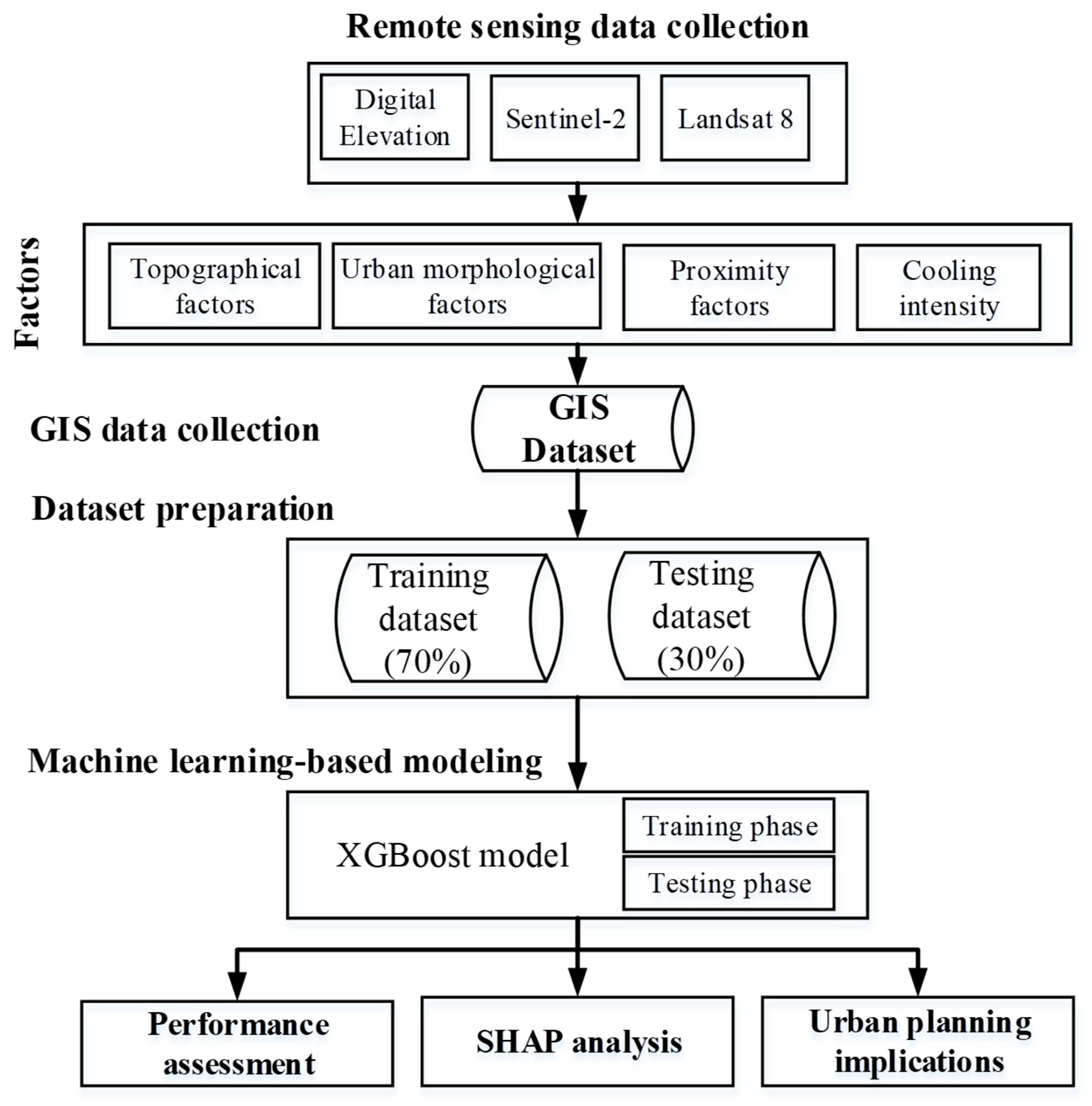
Figure 1. Schematic workflow of the study.
Sustainability 17 09824 g001
Figure 2. Study area as true color composite of Sentinel-2’s bands (Data source: European Union/ESA/Copernicus).
Sustainability 17 09824 g002
Figure 3. EVI map.
Figure 3. EVI map.
Sustainability 17 09824 g003
Figure 4. LULC map.
Figure 4. LULC map.
Sustainability 17 09824 g004
Figure 5. LST map.
Figure 5. LST map.
Sustainability 17 09824 g005
Figure 6. Cooling intensity map.
Sustainability 17 09824 g006
Figure 7. Topographical maps.
Sustainability 17 09824 g007
Figure 8. PLAND maps.
Sustainability 17 09824 g008aSustainability 17 09824 g008b
Figure 9. Maps of proximity features.
Sustainability 17 09824 g009
Figure 10. Prediction performance of XGBoost.
Sustainability 17 09824 g010
Figure 11. Maps of predicted cooling intensity: (a) XGBoost-based prediction and (b) prediction error.
Sustainability 17 09824 g011
Figure 12. Histograms of prediction error.
Sustainability 17 09824 g012
Figure 13. Results of REC.
Sustainability 17 09824 g013
Figure 14. Map of prediction error type.
Sustainability 17 09824 g014
Figure 15. Proportion of error types.
Sustainability 17 09824 g015
Figure 16. Feature assessment using SHAP: (a) SHAP’s impact plot and (b) Mean absolute SHAP value.
Sustainability 17 09824 g016
Figure 17. Partial dependency plots of blue-green PLAND indices: (a) shrubland, (b) tree canopy, and (c) waterbody.
Sustainability 17 09824 g017
Figure 18. Proportion of area according to cooling intensity (CI) category.
Sustainability 17 09824 g018
Figure 19. Cooling intensity (CI) reclassification.
Sustainability 17 09824 g019
Table 1. The employed remote sensing data.
DatasetTime PeriodBandsSpatial Resolution
Landsat 81 May 2024–30 September 2024SR_4, SR_5, and ST_B1030 m
NASA SRTM Digital Elevation 30 m Elevation30 m
Sentinel-21 January 2024–31 December 2024B2, B3, B4, B5, B6, B7, B8, B8A, B11, B1210 m (B2, B3, B4, and B8)
20 m (B5, B6, B7, B8A, B11, and B12)
Table 2. LULC classification performance.
LULC
Class
Accuracy
Rate
PrecisionRecallF1 ScoreCohen’s Kappa
Coefficient
Bareland0.890.880.890.890.85
Built-up0.890.880.890.890.85
Vegetation0.980.960.980.970.96
Waterbody0.960.990.960.970.97
Table 3. Statistical description of the collected GIS dataset.
VariableVariable NameUnitMinAverageMeanMax
X1Elevationm0.0022.0236.04291.35
X2Slopem0.004.994.8627.24
X3Aspect°0.00143.2341.97273.91
X4TPI--−12.140.001.6717.44
X5PLAND bareland%0.005.215.6352.67
X6PLAND shrubland%0.0014.1419.6597.33
X7PLAND tree canopy%0.0045.5731.42100.00
X8PLAND waterbody%0.0014.1123.42100.00
X9Distance to coastlinem144.7013,806.357219.5428,351.14
X10Distance to riverm0.001311.741209.196185.10
X11Distance to roadm9.73231.45354.862264.72
X12Distance to shrublandm0.65144.61153.201449.34
X13Distance to tree canopym0.0075.58179.461886.43
X14Distance to waterbodym0.00273.91269.162313.60
YCooling intensity°C−8.113.313.4613.20
Disclaimer/Publisher’s Note: The statements, opinions and data contained in all publications are solely those of the individual author(s) and contributor(s) and not of MDPI and/or the editor(s). MDPI and/or the editor(s) disclaim responsibility for any injury to people or property resulting from any ideas, methods, instructions or products referred to in the content.