Abstract
Urban mobility plays a critical role in ensuring resilience during natural disasters such as floods, yet developing reliable traffic models remains challenging for medium-sized cities with limited monitoring infrastructure. This study developed a hybrid traffic modeling approach that integrates Google Traffic data with field measurements to address incomplete digital coverage in flood-prone areas of Loja, Ecuador. The methodology involved collecting 1501 field speed measurements and 235,690 Google Typical Traffic observations using exclusively open-source tools and freely available data sources. Adjustment factors ranging from 0.25 to 0.97 revealed systematic discrepancies between Google Traffic estimates and field observations, highlighting the need for local calibration. The resulting traffic network model encompassing 4966 nodes and 5425 edges accurately simulated flood impacts, with the most critical scenario (Thursday 17–19, 100% road impact) showing travel time increases of 1123% and congestion index deterioration from 1.79 to 21.69. Statistical validation confirmed significant increases in both travel times (p = 0.0231) and distances (p = 0.0207) under flood conditions across five representative routes. This research demonstrates that accurate traffic models can be developed through intelligent integration of heterogeneous data sources, providing a scalable solution for enhancing urban mobility analysis and emergency preparedness in resource-constrained cities facing climate-related transportation challenges.
1. Introduction
Urban mobility plays a critical role in ensuring the resilience and functionality of modern cities, especially during natural disasters such as floods [1,2]. Although floods are a representative example, the need for reliable traffic models extends to any event that disrupts mobility, such as landslides, accidents, or road closures [3]. In such situations, reliable traffic models are essential to propose alternative routes and manage vehicular flows efficiently. However, the effectiveness of these models depends heavily on the accuracy and completeness of the input data [4]. This dependence underscores the urgent need for more precise and adaptive traffic modeling tools, particularly in regions vulnerable to extreme weather events.
Worldwide in many cities, including those in Latin America, developing detailed and up-to-date traffic models remains a significant challenge [5]. The construction of such models typically requires extensive infrastructure and resources, including sensors, monitoring systems, and personnel [6]. Consequently, cities often rely on publicly available platforms such as Google Traffic, which offer historical and real-time traffic data [7]. These platforms reduce the cost and time associated with data acquisition and modeling. Nevertheless, their utility varies widely depending on data availability and local conditions.
A frequent limitation observed in platforms like Google Traffic is the absence or incompleteness of traffic color codes in smaller or less-monitored cities [7,8]. This lack of detail restricts the ability to simulate traffic behavior accurately or respond dynamically to disruptions. In the case of Loja, a medium-sized city in southern Ecuador [9], these limitations have become particularly evident. During recent flood events between 2020 and 2025 [10,11,12,13], several key urban roads were submerged, and the absence of reliable traffic models led to widespread mobility chaos, with emergency services and daily commuters alike facing significant delays and uncertainty.
In response to these limitations, recent studies have increasingly focused on hybrid approaches that combine multiple traffic data sources to improve model reliability [14]. Merging digital traffic information with field-based observations allows for more context-aware models that better reflect real-world conditions [15]. This is especially relevant in flood-prone areas, where accessibility can change rapidly and unpredictably [16]. By supplementing general patterns captured digitally with localized field data, urban planners can improve the precision of their interventions and make better-informed decisions in real time.
Cities increasingly require traffic modeling tools that are both cost-effective and adaptable to rapidly changing conditions. In flood situations, delays in route reconfiguration can have severe consequences for public safety, logistics, and urban operations [17]. Therefore, integrating existing digital platforms with empirical data offers a practical and scalable solution [18] for medium-sized cities like Loja. This study addresses that need by exploring how traffic modeling can be enhanced through the combination of typical traffic patterns from Google Traffic and field-based measurements.
The objective of this study is to develop an improved urban traffic model applicable to various contexts of mobility disruption, with a particular emphasis on flood-prone areas such as Loja, by integrating freely available Google Traffic data with in situ traffic measurements. The methodology involved collecting typical traffic information from Google’s platform and conducting field observations on key road segments exposed to flooding. A comprehensive database was created, and missing segments were completed using previously calibrated traffic flow equations based on field trends [19]. This hybrid approach aimed to enhance the representativeness and utility of the traffic model under flood scenarios.
The results of this study have practical implications not only for emergency traffic management during floods but also for broader urban mobility planning in contexts where digital traffic data are limited or incomplete. The proposed methodology is replicable and scalable, offering a viable alternative for other mid-sized cities facing similar challenges. By demonstrating how low-cost data integration can produce more realistic traffic models, this study contributes to strengthening urban resilience and improving the effectiveness of mobility planning tools, both in flood scenarios and in a wider range of urban challenges.
2. Materials and Methods
2.1. Methodological Framework
The methodological approach implemented in this study follows a systematic five-stage framework designed to integrate multiple data sources and overcome the limitations of individual traffic information systems in medium-sized cities (See Figure 1). The five-stage framework consists of:
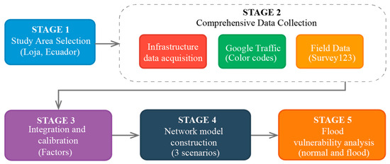
Figure 1.
Methodological framework for developing the hybrid traffic model in Loja, Ecuador.
- Study area selection and criteria establishment: Selection of Loja, Ecuador as the study area, based on specific criteria including limited Google Traffic coverage and documented flood vulnerability.
- Comprehensive data collection: Simultaneous acquisition of three data sources: (a) OpenStreetMap road network infrastructure using R programming environment, (b) Google Traffic typical conditions through systematic observation of color-coded traffic states, and (c) in situ speed measurements using Survey123 application across representative routes and time periods. All statistical analyses were performed in R 4.4.1 [20] using the RStudio 2024.04.1 environment [21].
- Data integration and calibration: Since Google’s service provides traffic conditions as color-coded information rather than direct speed values, traffic speeds were calculated using previously calibrated empirical equations. Application of adjustment factors derived from comparative analysis between field and Google Traffic speeds to harmonize heterogeneous data sources.
- Network model construction: Based on the corrected speed data, a traffic model was developed for the study area. The most unfavorable scenarios for the road network near the flood zone were identified, along with the most critical days and time slots for traffic conditions in the study area.
- Flood-Induced Traffic Vulnerability Analysis: Flood restrictions were implemented and a comparative route analysis was conducted to evaluate mobility impacts under both normal and flood-affected.
The methodology concludes with a hybrid traffic model for vulnerability assessment, which addresses three key challenges commonly encountered in traffic modeling for medium-sized cities.
2.2. Study Area Selection
The study was conducted in the city of Loja, located in southern Ecuador. This city was selected based on two main criteria: (1) the lack of complete Google Traffic color code coverage across its road network, and (2) its vulnerability to flooding due to the presence of multiple rivers and streams. Loja is a medium-sized urban center crossed from south to north by two principal rivers—Zamora and Malacatos—which converge near the historic center. This confluence zone is particularly critical, as it has experienced major flood events in recent years, disrupting areas with high socio-economic and transport relevance, such as schools, markets, and urban bus lines. Furthermore, Loja’s elongated shape along a north–south axis and its east–west traffic flows make this location especially important for analyzing traffic dynamics and vulnerabilities.
Figure 2 displays the coordinates −3.997385, −79.223754 and −3.974927, −79.185477 of the study site. This figure includes the approximate 2025 flood zone, calculated based on proximity to rivers and streams and informed by news reports. It’s important to note that this is a referential zone only and does not replace detailed hydraulic studies. The figure also highlights specific flood events reported in the news for 2020, 2021, and 2025 within this zone. Recently, Loja has experienced an increase in fluvial floods, a trend expected to continue given the impacts of climate change.
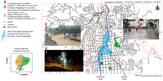
Figure 2.
Location map of Loja, Ecuador, highlighting the Zamora and Malacatos rivers and approximate 2025 flood zone and historical flood events [11,12,13].
2.3. Data Acquisition of Study Area Infrastructure
The spatial data required for traffic modeling in flood-prone areas of Loja, Ecuador, were obtained from OpenStreetMap (OSM) using the R programming environment (version 4.3.1). The analysis utilized several R packages: osmdata (v1.1.6) for querying and downloading OSM features, sf (v1.0-15) for handling spatial data, ggplot2 (v3.4.3) for map visualization, dplyr (v1.1.3) for data manipulation, openxlsx (v4.2.5) for Excel export, scales (v1.2.1) for scale management, and ggspatial (v1.1.8) for map annotations such as north arrows and scale bars.
A bounding box covering the study area was defined using the previous geographic coordinates of Loja. Streets, rivers, streams, buildings, green areas, and parks were queried and downloaded from OSM. Street data were processed to retain relevant attributes such as street name, type, surface, lanes, maximum speed, and accessibility, with missing values standardized for consistency. The cleaned dataset was exported to Excel for further analysis and integration with field-collected traffic data.
2.4. Collection of Google Traffic Data
Google Traffic data were acquired through systematic manual observation of the platform’s color-coded traffic conditions across Loja’s road network within the defined study polygon. Given that Google does not provide public API access to historical traffic color-code data, a manual observation protocol was implemented. Couple trained observers worked in coordinated shifts to record traffic states at predetermined geographic coordinates during representative time periods, capturing typical urban mobility patterns throughout a complete weekly cycle.
The observation protocol involved: (1) defining a grid of observation points covering the study area; (2) establishing a standardized recording template (see Table 1 for an example); (3) training observers on consistent color identification; and (4) implementing quality control checks for data consistency. Observers used the Google Maps web interface to visually inspect traffic conditions at each location and systematically recorded the displayed color code. While this approach is labor-intensive, it was feasible for our focused study area (approximately 10 km radius polygon) and provided direct access to Google’s traffic classification system without requiring proprietary data agreements.

Table 1.
Data structure example for Google Traffic observations.
Traffic conditions were classified according to Google’s standard color coding system: green (free flow), yellow (moderate congestion), orange (heavy congestion), red (severe congestion), and cases where no color information was available (labeled as “None”). Data were collected using this standardized sampling approach every 15 min across all seven days of a typical week, ensuring comprehensive temporal coverage of traffic patterns.
2.5. Field Data Collection Using Survey123
In the second stage, field measurements were collected using the Survey123 mobile application. The tool was installed on a GPS-enabled smartphone, which automatically recorded geographic coordinates, date, and time. The operator, traveling in taxis or personal vehicles, only needed to manually input the vehicle’s speed during each trip. Data were collected on several streets near flood-prone areas between 7 July and 18 July 2025. Measurements were taken during high-traffic periods, specifically from 07:00 to 24:00, to capture mobility patterns associated with daily routines (commuting, school, commercial activity) and nightlife.
A total of 1507 records were obtained (see Figure 3). Data cleaning was then applied to ensure quality. One record was discarded for falling outside the study area, and five were removed due to inconsistent entries with missing speed values. Observations with speeds exceeding 100 km/h were excluded as they were considered unrealistic for urban areas. Additionally, entries with inconsistent or missing timestamps, as well as those outside the defined temporal window, were discarded. After these filtering steps, the final dataset comprised 1501 validated and georeferenced speed records. All original data presented in this study are publicly available. The download link is provided in the Data Availability Statement at the end of this document.
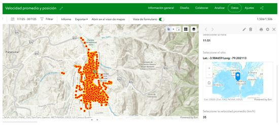
Figure 3.
Screenshot of the Survey123 interface used for recording traffic speed.
2.6. Spatial Assignment of Ground Speed Data to Road Segments
To associate the field-collected speed observations with road segments from OSM, a custom algorithm was developed in the R programming language. This process relied on the readxl (1.4.3), writexl (1.4.2), dplyr (1.1.4), and ggplot2 (3.4.4) packages. Two datasets served as inputs: the Speeds dataset, which contained 1501 georeferenced points (longitude, latitude) with corresponding speed values (km/h), and the Streets dataset, which comprised OSM road segments with attributes like street name and street type.
The algorithm worked by computing the Euclidean distance from each point in the Speeds dataset to every road segment. This was achieved by projecting the point onto the line defined by the start and end coordinates of each segment. The perpendicular distance was calculated if the projection fell within the segment; otherwise, the distance to the nearest endpoint was used. The road segment with the minimum distance was then assigned as the most likely location of that speed observation.
To enhance reliability, only points located within 20 m (approximately 0.00018 decimal degrees) of a road segment were retained. This threshold accounts for common GPS positional errors and reduces the risk of incorrectly assigning points to parallel or nearby roads, which is a common issue in dense urban areas. Given that the study area spans a relatively small radius of approximately 10 km, the Euclidean distance was chosen over the Haversine formula, offering greater computational efficiency without compromising geographic accuracy.
To quantitatively validate the use of Euclidean distance instead of the Haversine formula, we compared both methods for 500 randomly selected point pairs within the study area. The maximum difference between Euclidean and Haversine distances was 0.007 m (mean = 0.004 m, SD = 0.002 m), which represents less than 0.04% of the 20-m spatial assignment threshold. Therefore, the Euclidean approach introduces an error well below the GPS positional uncertainty (± 5–10 m) and can be considered negligible for the study’s spatial scale.
2.7. Deriving Adjustment Factors for Google Traffic Data
To harmonize the different sources of traffic information, Google Maps’ traffic colors were first converted into speed values. This was accomplished using specific equations for the city of Loja, which a previous study developed to relate speed, density, and flow to each Google traffic color [19].
Once the Google speeds were established, field measurements were systematically compared with these Google Traffic observations. Adjustment factors were then calculated as the ratio between the field-measured speeds and the Google-reported average speeds. These factors were stratified by road type and time slot to capture both spatial and temporal variability.
This integration process was conducted in R using the dplyr (v1.1.4) and tidyr (v1.3.0) packages, supported by visualizations that highlighted systematic deviations between both data sources. The application of these adjustment factors allowed for the correction of Google Traffic estimates, ensuring the final model incorporated both the broad coverage of Google’s data and the high accuracy of the field observations.
2.8. Construction of the Traffic Model
Following the correction of Google Traffic data using field-derived adjustment factors, the estimated speeds were assigned to corresponding OSM road segments. These speeds were subsequently aggregated by road segment, day, and time slot, thereby creating a comprehensive dataset with time-dependent travel speed estimates for each street.
To model the road network, a weighted graph was constructed using the igraph package in R. The graph’s nodes were defined by the coordinates of the road segment vertices, while the edges represented the segments connecting them. Each edge was assigned a weight equivalent to travel time, which was calculated by dividing the segment’s length by its corrected average speed.
2.9. Flood Vulnerability Analysis
Building on the constructed urban mobility graph, a simulation model was implemented to evaluate the road network’s vulnerability to flood events. The analysis began by defining a flood-prone area based on historical reports and georeferenced points. This area was represented by a closed polygon, which was integrated into the traffic model to simulate accessibility disruptions during river overflow events. The polygon was constructed from the following coordinates:
- −3.996987, −79.205434;
- −3.996937, −79.204867;
- −3.993843, −79.205167;
- −3.993660, −79.203950;
- −3.991896, −79.204233;
- −3.991447, −79.200881;
- −3.988516, −79.202524;
- −3.987450, −79.202311;
- −3.986981, −79.201769;
- −3.986413, −79.201869;
- −3.985347, −79.201841;
- −3.985119, −79.201769;
- −3.983883, −79.202068;
- −3.983329, −79.203066;
- −3.985446, −79.204305;
- −3.988118, −79.204177;
- −3.989738, −79.205901;
- −3.991017, −79.205516;
- −3.991785, −79.206057;
- −3.995252, −79.205815.
The flood polygon was derived from documented historical flood reports and media sources because no official hydrodynamic model or high-resolution flood map is currently available for Loja. While this approach captures the main areas historically affected by river overflows, we acknowledge that it does not fully represent hydraulic processes such as water depth or flow velocity. Future work could incorporate two-dimensional hydrodynamic modeling (e.g., HEC-RAS 2D or LISFLOOD-FP) or GIS-based inundation mapping using digital elevation data to refine spatial accuracy and enhance reproducibility.
To assess the impact on mobility, three distinct flood scenarios were simulated for the most critical days and time slots previously identified. These scenarios represented a severe flood (100% of affected roads), a moderate flood (75%), and a minor flood (50%). The flood’s effect was modeled by applying a 100-fold travel time penalty to all road segments within a 200-m buffer around the flood polygon. The selection of these parameters was based on the following considerations:
- 200-m buffer zone: This distance was determined by: (1) typical urban block dimensions in Loja, which range from 150–250 m based on OSM infrastructure analysis; (2) documented flood impact zones in similar urban contexts [22,23]; and (3) the practical extent of mobility disruption beyond directly inundated areas, where access restrictions, emergency vehicle presence, and precautionary closures extend the effective impact zone.
- 100-fold travel time penalty: This penalty magnitude was calibrated to: (1) effectively force shortest-path algorithms to seek alternative routes around flooded areas; (2) maintain computational stability while representing severe disruption; (3) align with approaches documented in urban network disruption studies where penalties of 50−150x are commonly applied [24,25]. This penalty simulates near-total inaccessibility rather than complete road removal, which better reflects real-world conditions where emergency vehicles may still access affected areas.
- 30 km/h default speed: For segments lacking traffic data from both Google and field sources, a conservative default speed of 30 km/h was assigned based on: (1) the observed mean field speed of 34.16 km/h across all collected measurements; (2) adjusting downward to avoid overestimating network capacity in data-sparse segments; and (3) consistency with typical urban residential street speeds in similar Latin American cities.
To quantify the impact of these scenarios, three key metrics were calculated:
- Average Travel Time (ATT): The average travel time across all road segments in the network.
- Total Affected Length (TAL): The cumulative length of all road segments impacted by the flood.
- Average Congestion Index (ACI): A measure of congestion severity, defined as the ratio of free-flow speed to effective travel speed:
The entire analysis and simulation were performed using the R using key packages included sf (v1.0−15) for spatial data handling, dplyr (v1.1.4) and tidyr (v1.3.0) for data manipulation, osmdata (v1.1.6) for OSM data retrieval, and igraph (v1.5.1) for network modeling. Visualization was handled with ggplot2 (v3.4.4), with plots saved using svglite (v2.1.3). Additional functionalities were provided by geosphere (v1.5−19) for geographic calculations, RColorBrewer (v1.1−4) for color palettes, openxlsx (v4.2.5) for data input, and progress (v1.2.3) for process tracking.
2.10. Flood Scenario Analysis
Building on the criticality analysis, a comparative study was conducted to evaluate urban mobility under both normal (no flood) and flood conditions, focusing on the most unfavorable day and time slot previously identified. For this evaluation, five representative routes were defined within the study area to capture different mobility patterns.
The chosen routes, which include central corridors prone to flooding as well as connections between peripheral neighborhoods and areas of high commercial or service interest, are:
- Route 1: from (−3.992463, −79.208158) to (−3.990998, −79.199949);
- Route 2: from (−3.986847, −79.208441) to (−3.993072, −79.199652);
- Route 3: from (−3.995702, −79.209686) to (−3.985434, −79.201347);
- Route 4: from (−3.983043, −79.211539) to (−3.978088, −79.201166);
- Route 5: from (−3.977500, −79.204925) to (−3.996355, −79.202094).
As a reference for validation, the distance and travel time for each route were also obtained from Google Maps on 12 September 2025, between 17:00 and 19:00, and were later compared with the model’s metrics under normal conditions.
The flood polygon used for the simulation was the same one defined in the previous vulnerability analysis. The selected time slot represents the most critical mobility conditions in Loja, as it coincides with peak-hour traffic flow, commercial activity, and vulnerability to flood-induced disruptions. By focusing on this scenario, the model’s ability to simulate urban resilience under the most challenging traffic conditions was evaluated.
The flood’s impacts on mobility were assessed through paired comparisons of route performance before and after applying the restrictions. The indicators analyzed were travel time and route distance, which directly reflect the accessibility and efficiency of mobility during a disruption. Observed differences in mobility metrics were statistically evaluated to determine their significance, using paired Student’s t-tests with a 95% confidence level, implemented in R.
The validation through five representative routes was designed to reflect diverse traffic contexts. However, we acknowledge that broader network validation would provide more robust performance metrics. Future work could implement Monte Carlo simulations using random origin–destination pairs and compare simulated vs. observed travel times to strengthen external validity.
3. Results
3.1. Study Area Infrastructure
The study area’s road network, extracted from OSM, consists of 1050 segments with a total length of 172.91 km. Segment lengths exhibit substantial variability, ranging from 0.63 m to 3403.06 m, with a mean of 164.67 m and a median of 97.11 m. Classification by street type indicates a predominance of residential streets (66.8%), followed by service roads (12.8%), primary roads (10.4%), secondary roads (5.1%), tertiary roads (3.6%), and unclassified segments (1.3%). This distribution reflects the urban morphology of Loja, characterized by a dense network of local streets interspersed with arterial and collector roads.
3.2. Field Speed Data
As a result of the vehicle speed measurements collected on urban streets in the city of Loja, the dataset shows a standard deviation of 13.53 km/h, an average speed of 34.16 km/h, a maximum speed of 70 km/h, and a minimum speed of 0 km/h (recorded only once). Zero-speed value indicates a location where congestion caused the recording vehicle to come to a complete stop.
The distribution of speeds, grouped in 10 km/h intervals, is shown in Figure 4, together with the corresponding response rate (%) for each range. Results indicate that most observations fall between 10 and 40 km/h, consistent with a previous study in the same city, where traffic data were collected between 06:00 and 22:00 [19].
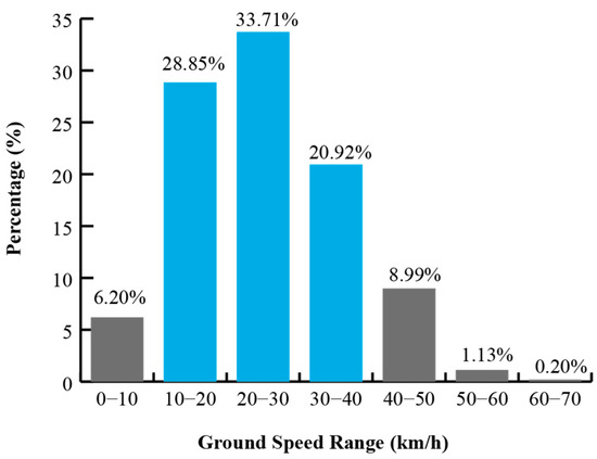
Figure 4.
Distribution of collected ground speed measurements by 10 km/h intervals.
Regarding the temporal distribution of the data, records were collected from 07:00 to 24:00, as shown in Figure 5A. The time slots with the highest number of records were 11:00–12:00 and 18:00–19:00 (both exceeding 17%), which typically coincide with peak traffic hours. Figure 5B presents the percentage of records collected by day of the week. The largest share corresponded to Friday (43%), followed by Tuesday (21%) and Thursday (19.4%). These variations across time periods and weekdays do not significantly affect the analysis, since the aim was to achieve broad coverage throughout the day and across the entire week.
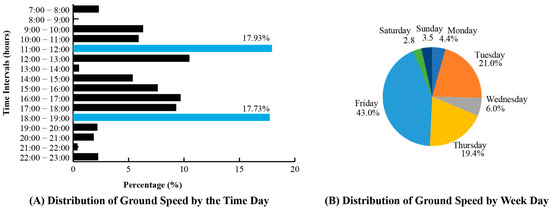
Figure 5.
Temporal distribution of collected ground speed measurements.
3.3. Typical Traffic Data from Google Data
The Google traffic data distribution is presented in Figure 6, showing the speed characteristics across the study area. Unlike field measurements, temporal distribution analysis was not required for Google data due to its systematic collection methodology. Data were automatically collected every 15 min throughout all days and time ranges, ensuring uniform temporal coverage with exactly four records per hour and equal representation across all weekdays (14.29% each day).
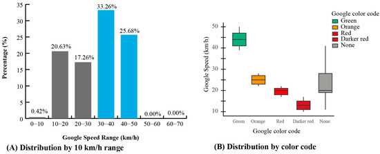
Figure 6.
Google traffic speed distributions in the study area.
The statistical analysis of Google traffic speeds revealed a mean velocity of 36.84 km/h with a standard deviation of 11.01 km/h. The speed range extended from a minimum of 10 km/h to a maximum of 55 km/h, demonstrating a more constrained distribution compared to field observations. The speed distribution, grouped in 10 km/h intervals, shows that most Google traffic speeds fall within the 26–50 km/h range, reflecting typical urban driving conditions under normal traffic flow (See Figure 6A).
This uniform temporal distribution makes Google traffic data particularly valuable for establishing baseline traffic conditions across different time slots and days, providing a robust foundation for the adjustment factor calculations that harmonize field and Google observations into a coherent traffic model.
On the other hand, a typical Google Traffic color distribution shows that green corresponds to higher speeds than yellow, red, and dark red (See Figure 6B). This is consistent with the Highway Capacity Manual (HCM) and real-world conditions. The “none” category shows greater variability, meaning that speeds were assigned based on the range from the preliminary study, since no specific speed data was available.
3.4. Estimation of Average Speed from Google Data
A previous study in the city of Loja established equations relating speed, density, and flow for the different Google Maps traffic colors [19]. These twelve equations (six for flow, q, and six for speed, s) are detailed in the referenced article and are categorized according to the traffic indicator associated with the color code. This earlier work also established the relationship between speed and the urban street Level of Service (LOS) defined by the TRB [26], classifying the analyzed roads as Urban Street Class III, which has a typical Free Flow Speed (FFS) of 50 km/h.
According to the same study, Google traffic colors can be associated with LOS levels as follows: A and B (green), C and D (orange), E (red), and F (dark red). Since Google provides color codes rather than explicit speed values, random speeds were assigned to each color based on the corresponding LOS category. For road segments without traffic color information, random speeds between 15 and 55 km/h were also assigned—following the ranges reported in the previous study. This “no color” condition typically reflects streets with limited user location data.
Using these assigned speeds and the equations from the earlier study, traffic density (veh/km) was estimated, and subsequently, traffic flow (veh/h) was derived. Equation thresholds were respected during the calculations: if a computed value fell outside the valid range, the corresponding minimum or maximum was applied.
The results of these calculations, together with the theoretical relationships, are presented in Figure 7. In the case of the traffic flow versus traffic density plot, only a single branch is available, which nevertheless supports the plausibility of the obtained values.
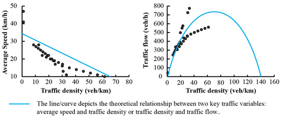
Figure 7.
Theoretical and calculated relationships between speed, density, and flow for urban streets in study area.
3.5. Traffic Data Integration
A crucial first step was to assign the collected field and Google traffic data points to the OSM road network. This process involved matching each georeferenced point to the nearest road segment, a critical step to ensure that speed observations were accurately integrated into the urban model.
Out of the 1501 field-collected points, 1334 (88.9%) met the distance criterion and were successfully assigned to the street network (See Figure 8). Distances for these points ranged from nearly zero to the 20-m threshold, with an average of approximately 4.8 m and a median of 3.2 m. By street type, most points were on residential streets (48.8%), followed by primary roads (31.3%) and tertiary roads (9.2%). A street-level analysis revealed variations in average speeds; for instance, 8 de Diciembre Avenue had a mean speed of 35.4 km/h (47 points), while 10 de Agosto Avenue showed a lower average of 23.4 km/h (43 points), reflecting different traffic conditions.
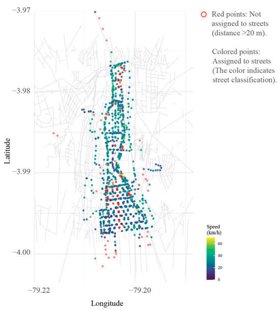
Figure 8.
Speed distribution based on proximity to OpenStreetMap streets (GPS-assigned streets).
Similarly, Google traffic observations, totaling 237,510 data points, were successfully matched to the OSM street network within the defined distance threshold of 20 m. This extensive dataset achieved a remarkable assignment rate of 99.2%, with 235,690 points successfully integrated into the network model.
3.6. Adjustment Factors
Adjustment factors represent the ratio between the mean field (ground) speed and the mean Google-derived speed. Before calculating these factors, a comparison of average speeds from both sources was conducted, as illustrated in the boxplot in Figure 9. This comparison, stratified by street type, shows that Google-reported speeds tend to display greater variability than field measurements. Moreover, field data generally indicate lower average speeds across most street types when compared with Google Traffic.
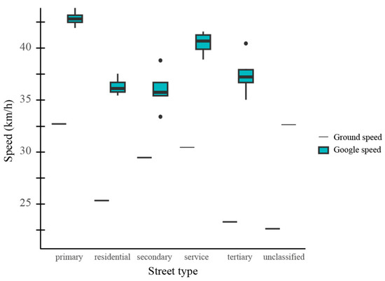
Figure 9.
Boxplot of field speeds and Google-estimated speeds by street type.
If a simple ratio of average speeds were applied, the resulting correction would overestimate speeds in lower ranges and underestimate them in higher ranges. To address this issue, adjustment factors were calculated separately for each street type and time slot. The time slots were defined as follows: 06:00–08:00, 08:00–12:00, 12:00–14:00, 14:00–17:00, 17:00–19:00, and 19:00–06:00, corresponding to the city’s commuting, commercial, and nighttime activity patterns. Additionally, time slots were defined to aggregate field observations into representative periods. Attempting to collect one record every 15 min across the entire network—as Google does—would require an unfeasible amount of data; therefore, this study aims to simplify data collection while still capturing the main temporal dynamics of urban mobility.
The resulting factors are summarized in Table 2, which presents the mean field speeds, mean Google-derived speeds, and their ratio (Adjustment Factor), along with a heatmap illustrating the variation of adjustment factors across street types and time slots (Figure 10). The extreme value (0.25) observed for service roads between 14:00–17:00 likely reflects localized anomalies such as temporary closures or a small sample size. The lowest factors correspond to segments with minimal observations, indicating that higher variability arises from data sparsity rather than measurement error, and these results are reported in Table 2 with sample sizes and confidence intervals.
Table 2.
Calibration factors for Google traffic speed by street type and time-of-day.
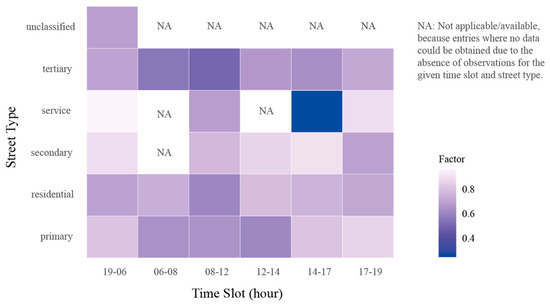
Figure 10.
Heatmap of adjustment factors by street type and time slot.
Table 2 presents the adjustment factors calculated as the ratio between field-measured speeds and Google-derived traffic speeds across different street types and time slots. These factors are essential for correcting discrepancies between the two data sources and for producing a reliable traffic network model. The results indicate a systematic difference between field and Google speeds. For primary roads, adjustment factors range from 0.61 to 0.86, with the lowest values occurring during morning and midday periods (06–08 and 12–14), reflecting slower field speeds relative to Google estimates during peak congestion hours. Evening and night periods (19–06 and 17–19) show higher factors, indicating closer agreement between field and Google speeds.
Residential streets exhibit similar patterns, with adjustment factors between 0.61 and 0.79. Lower factors are observed in the morning (08–12) and late afternoon (17–19), suggesting that Google traffic data may overestimate actual speeds in densely populated areas during these periods.
For secondary and tertiary roads, adjustment factors vary more widely. Secondary roads range from 0.70 to 0.90, while tertiary roads show a wider spread (0.50–0.72), particularly during morning and midday periods when field speeds are significantly lower than Google speeds. This highlights the importance of context-specific correction factors for lower-hierarchy roads, which are more sensitive to local traffic conditions.
Service roads display the most variability, with adjustment factors ranging from 0.25 to 0.97. The extremely low factor of 0.25 during the 14–17 time slot indicates substantial discrepancies between field measurements and Google data, possibly due to local disruptions, temporary closures, or underestimation of congestion by Google.
Overall, these adjustment factors reveal that Google-derived traffic speeds tend to overestimate real-world conditions, particularly during peak hours and on lower-capacity streets. Applying these factors is crucial for generating realistic travel time estimates, congestion indices, and network simulations, ensuring that the modeled scenarios accurately reflect actual urban mobility.
The adjustment factors derived in this study represent short-term conditions based on data collected during a two-week period in July 2025. Although no significant weather or road maintenance variations were reported during that period, the stability of these factors over longer timeframes (e.g., seasonal or annual) was not directly evaluated. Therefore, they should be interpreted as temporally representative of typical dry-season conditions. Future studies could extend this analysis to examine potential temporal variability of adjustment factors under different seasonal or traffic conditions.
3.7. Traffic Network Model Construction
The traffic network model was constructed by integrating corrected traffic speeds into a comprehensive graph-based representation of the study area’s road infrastructure. The final model encompassed 4966 nodes and 5425 edges, covering a total road network length of 165.35 km across Loja’s urban area. The script used for this analysis is provided in the Supplementary Materials.
Speed aggregation was performed systematically for all road segments across different temporal dimensions, incorporating the seven days of the week and six time slots (06−08, 08−12, 12−14, 14−17, 17−19, and 19−06). The established adjustment equations between field measurements and Google traffic data were applied to supplement missing speed information, ensuring comprehensive coverage of the network. For segments lacking any traffic data, a conservative default speed of 30 km/h was assigned, based on typical urban driving conditions in similar contexts and Google’s typical traffic patterns.
Travel times were calculated using the corrected speeds and segment lengths, creating a weighted graph structure optimized for shortest-path algorithms. The Dijkstra algorithm was implemented for route optimization and travel time calculations, providing the computational foundation for the flood impact simulations.
3.8. Criticality Analysis and Scenario Definition
The identification of critical traffic scenarios was based on a comprehensive analysis of traffic density and flow patterns across temporal dimensions. A criticality score was computed for each day-time slot combination, incorporating average traffic density, average flow, and the number of observations to ensure statistical robustness.
The analysis revealed distinct patterns in urban mobility, with evening peak hours (17–19) consistently ranking highest across multiple weekdays. The top three critical scenarios identified were:
- Thursday 17–19: The most critical scenario with a criticality score of 109.5, characterized by an average density of 8.46 and average flow of 210.5 observations.
- Tuesday 17–19: The second most critical scenario (criticality score: 106.3), with an average density of 8.16 and average flow of 204.5 observations.
- Friday 17–19: The third critical scenario (criticality score: 105.8), showing an average density of 8.15 and average flow of 203.4 observations.
The comprehensive criticality analysis across all 42 day-time slot combinations reveals distinct temporal patterns in urban mobility demand. Evening peak hours (17–19) consistently dominate the highest criticality rankings, with all weekdays (Monday through Friday) appearing in the top 10 scenarios, reinforcing the concentration of traffic demand during typical commuting hours. Midday periods (12–14 and 14–17) also demonstrate elevated criticality scores, particularly on weekdays, with Friday 12–14 ranking sixth (102.5) and multiple 14–17 time slots appearing in the top 15. Weekend patterns show markedly different characteristics, with Saturday scenarios generally ranking in the middle tier (criticality scores ranging from 82.9 to 96.9), while Sunday consistently shows the lowest criticality across all time slots, with scores ranging from 79.5 to 89.7. Early morning periods (06–08) exhibit the lowest criticality scores across all days, ranging from 79.5 (Sunday) to 85.2 (Thursday), indicating minimal traffic demand during these hours. The overnight period (19–06) shows moderate criticality levels, with weekday scores ranging from 90.1 to 96.8, suggesting sustained but reduced traffic activity. This comprehensive temporal analysis confirms that flood impacts would be most severe during weekday evening peaks, while weekend mornings and all overnight periods would experience relatively lower disruption levels.
These scenarios represent the temporal windows when the road network operates at maximum capacity, making them particularly vulnerable to external disruptions such as flood events. The concentration of critical scenarios during evening peak hours (17–19) across weekdays reflects typical urban commuting patterns and validates the temporal focusing of the flood impact analysis.
The flood impact simulation was conducted using three distinct scenarios representing varying degrees of infrastructure disruption: 100% road impact (complete obstruction), 75% road impact (severe disruption), and 50% road impact (moderate disruption). Each flood scenario was evaluated against its corresponding no-flood baseline to isolate the specific impacts attributable to flooding (see Figure 11). It is important to clarify the interpretation of the flood scenario percentages. The “100% impact scenario” signifies that 100% of the road segments within the predefined flood-prone polygon experience severe disruption (a 100-fold travel time penalty), not that 100% of the city’s entire road network is affected. The 75% and 50% scenarios, in turn, affect progressively smaller portions of the network by randomly selecting subsets of segments within this flood zone for penalty application. This approach allows for a systematic evaluation of how flood severity scales affect network-wide mobility, while preserving geographic realism by concentrating impacts in the historically flood-prone area.
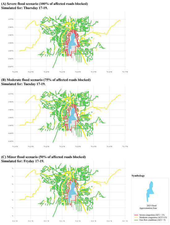
Figure 11.
Simulation of critical traffic scenarios under varying levels of flood impact.
The simulation results demonstrate a pronounced impact on average travel times (ATT) across all flood scenarios. The most severe case, the 100% road impact scenario occurring during Thursday’s evening peak (17–19), resulted in an ATT of 4.29 min, representing a dramatic increase of 3.93 min (1123%) compared to the baseline ATT of 0.35 min. The 75% impact scenario, simulated during Tuesday’s evening peak, showed an ATT of 3.49 min, representing an increase of 3.14 min (897%) over the baseline. Even the most moderate flood scenario (50% impact on Friday 17–19) demonstrated significant disruption, with an ATT of 2.47 min—a 2.12-min increase (606%) above baseline conditions.
The Total Affected Length (TAL) metric provides insight into the physical extent of network disruption. The 100% impact scenario affected 36.01 km of the road network (21.8% of the total 165.35 km), while the 75% and 50% scenarios affected 24.78 km (15.0%) and 19.71 km (11.9%), respectively. This progressive relationship between flood intensity and affected network length demonstrates the cascading nature of flood impacts on urban infrastructure.
The Average Congestion Index (ACI) revealed the most dramatic changes, serving as a sensitive indicator of network-wide traffic conditions. Under baseline conditions, all scenarios maintained an ACI of approximately 1.79, indicating free-flow conditions. However, flood scenarios triggered substantial congestion increases:
- 100% impact scenario: ACI reached 21.69, representing an increase of 19.90 points (1112% increase);
- 75% impact scenario: ACI rose to 17.68, an increase of 15.88 points (887% increase);
- 50% impact scenario: ACI increased to 12.51, representing a rise of 10.72 points (599% increase).
The comparative analysis reveals a clear relationship between flood intensity and network disruption. The Thursday 17–19 scenario, identified as the most critical through the criticality analysis, experienced the most severe impacts across all metrics. This validates the methodology for identifying vulnerable temporal windows and demonstrates the compounding effect of high baseline traffic demand with external disruptions. The results indicate that even moderate flood events (50% impact) can severely compromise urban mobility, with travel time increases exceeding 600% and congestion index rises of nearly 600%. This high sensitivity to disruption highlights the vulnerability of urban transportation networks in intermediate cities, where limited redundancy and alternative routes amplify the impact of infrastructure failures. The progressive nature of impacts across scenarios provides valuable insights for emergency management and urban planning, demonstrating that flood intensity directly correlates with mobility disruption magnitude across multiple performance metrics.
3.9. Performance of Critical Routes
The analytical script used for route analysis is included in the Supplementary Materials. Five representative routes were evaluated under both normal traffic conditions and a simulated flood event during the critical period of Thursday 17:00–19:00.
Performance metrics for both scenarios are summarized in Table 3, which includes route distances, travel times, and average speeds. Under normal conditions, route lengths ranged from 3.79 km to 7.06 km, with travel times between 8.93 and 16.60 min. Route 3 exhibited the longest distance and travel time, reflecting its trajectory through central areas with lower average speeds. The spatial representation of both “before” and “after” routes is shown in Figure 12.
Table 3.
Comparison of route performance metrics under normal and simulated flood conditions for proposed model.
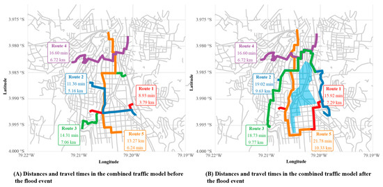
Figure 12.
Comparison of distances and travel times for five representative routes. The figure shows the traffic metrics before and after the flood event during the Thursday 17:00–19:00 time slot.
Flood restrictions were simulated by applying a 100-fold increase in travel time within the designated flood polygon. This resulted in significant changes in optimal routes, as the shortest-path algorithm rerouted traffic around the affected areas. As shown in Table 3, the post-flood metrics reveal substantial impacts. Route 5 was the most affected, with its travel time increasing by 8.51 min and total distance increasing by 4.09 km. Route 4 was notably unaffected, as its original path did not pass through the flood zone.
Paired t-tests confirmed that flood events produced statistically significant increases in both travel times and distances. Travel times increased by an average of 5.51 min per route (t = −3.582, df = 4, p = 0.0231; 95% CI: −9.79 to −1.24 min), while route distances increased by an average of 2.95 km per route (t = −3.710, df = 4, p = 0.0207; 95% CI: −5.17 to −0.74 km).
These results provide robust evidence that flood events substantially disrupt urban mobility during the Thursday 17:00–19:00 critical period, emphasizing the importance of alternative route planning and emergency management strategies in flood-prone areas. The rerouted paths and affected road segments are highlighted in the combined visualization presented also in Figure 12.
3.10. Methodology Extrapolation and Scaling Approaches
While this study focused on a representative portion of Loja’s road network, the developed methodology can be extrapolated to analyze city-wide traffic disruptions under flood scenarios. The most straightforward approach involves applying the field-measured average speeds directly to the complete OSM road network by extracting all road segments from the city’s database and systematically assigning the measured average speeds based on corresponding time slots and street types established in this study. This method leverages the established speed-street type relationships without requiring additional data collection, making it immediately implementable, though it assumes spatial homogeneity in traffic patterns across different urban zones.
A second approach utilizes the calibration factors developed in this study combined with comprehensive Google traffic data collection across the entire road network. This method requires systematic acquisition of Google’s typical traffic database for all network segments, which, while time-intensive when performed manually, provides comprehensive spatial coverage and captures spatial variations in traffic patterns while maintaining consistency with local field observations through the adjustment factors. The primary limitation is the substantial data collection effort required for manual acquisition of Google traffic information across an entire city network.
The third approach involves strategic sampling of representative locations across different urban zones, street types, and time periods, requiring calculation of average speeds for different combinations of days, hours, and street classifications through targeted data collection at spatially distributed sampling points. The sampling strategy would ensure coverage of various urban contexts while maintaining statistical representativeness across all time slots, with equations from the previous study applied to generate comprehensive traffic maps for the entire city. This approach optimizes the balance between data collection effort and spatial representativeness, making it particularly suitable for resource-constrained research environments.
The selection of the most appropriate scaling approach should consider local research capabilities, available resources, and required accuracy levels. The direct extrapolation method offers immediate implementation but may sacrifice spatial precision, the Google traffic integration approach provides comprehensive coverage but requires substantial resources, while the representative sampling method balances accuracy with feasibility. Regardless of the chosen method, the fundamental methodology developed in this study provides a robust framework for city-wide traffic disruption analysis under flood scenarios.
4. Discussion
The implementation of a hybrid approach that integrates Google Traffic data with field measurements represents a significant advancement in traffic modeling for medium-sized cities with limited monitoring infrastructure. The results demonstrate that the proposed methodology effectively addresses deficiencies in free digital platforms, particularly in urban contexts where traffic color-code coverage is incomplete. The calculated adjustment factors ranging from 0.25 to 0.97 reveal systematic discrepancies between Google Traffic estimates and field-observed speeds, with the most pronounced variations occurring during peak hours and on lower-capacity streets. These findings highlight the critical importance of locally calibrating digital data, especially in cities where mobility patterns may differ substantially from those assumed in Google’s traffic algorithms [27,28].
The temporal variability in adjustment factors indicates that discrepancies between data sources are not constant but fluctuate according to specific traffic conditions. Lower factors (<0.8) during morning hours (06−08 and 08−12) and the 17−19 time slot demonstrate that Google Traffic tends to overestimate speeds under both free-flow and moderate congestion conditions. This dynamic behavior underscores the need for time-sensitive calibration when applying hybrid models in similar urban contexts. The successful integration of 88.9% of field speed points and 99.2% of Google Traffic observations into the OpenStreetMap road network validates the robustness of the spatial assignment algorithm developed. The 20-m threshold proved appropriate for the urban setting, balancing geographic accuracy with GPS errors typically ranging from 20–23 m in dense areas [29,30,31]. Comparisons with Google Maps routes showed close agreement in distance and travel time, confirming the model’s validity, while minor differences reflected the integration of local information absent in commercial platforms.
The flood impact simulation results reveal the extreme vulnerability of Loja’s urban mobility system to flood events. The most critical scenario (Thursday 17−19, 100% road impact) demonstrated travel time increases of up to 1123%, with the Average Congestion Index rising from 1.79 to 21.69. These dramatic changes validate the model’s capability to simulate realistic mobility disruptions under extreme events. The progressive relationship between flood intensity and network disruption—with 100%, 75%, and 50% scenarios affecting 21.8%, 15.0%, and 11.9% of the road network, respectively—demonstrates the cascading nature of flood impacts on urban infrastructure [22,23].
Statistical analysis through paired t-tests confirmed that flood restrictions produced statistically significant increases in both travel times (p = 0.0231) and route distances (p = 0.0207) across the five representative routes analyzed. Route 5 experienced the most severe impact with an 8.51-min increase in travel time and 4.09 km additional distance, while Route 4 remained unaffected as it did not traverse the flood zone. This variability illustrates the importance of route-specific vulnerability assessment in emergency planning [24,25].
The methodology’s reliance on free and open-access data sources (OpenStreetMap, Google Traffic) and open-source tools (R, Survey123) reduces barriers to adoption in resource-limited cities. The adjustment-factor approach by road type and time slot is transferable to other contexts, though it requires local calibration to account for unique mobility patterns. This adaptability represents both a strength—due to its flexibility—and a limitation, given the need for local fieldwork [32,33].
Several aspects of our field data collection methodology warrant explicit discussion regarding representativeness and potential biases. The temporal distribution shows an overrepresentation of Friday observations (43% of total), which resulted from logistical constraints during the July 2025 field campaign when coordination with available vehicles was most effective. However, three factors mitigate concerns about systematic temporal bias affecting our results: First, our primary analytical objective was capturing spatial variations in speed across different road segments and street types rather than modeling precise temporal traffic dynamics—the adjustment factor methodology specifically addresses temporal calibration by correcting field observations against Google’s systematically collected data across all days and time periods. Second, the most critical time slot identified (Thursday 17−19) was well-represented in our field data collection (127 observations), providing robust calibration for the scenarios most relevant to our flood impact analysis.
The manual observation methodology for Google Traffic data collection, while providing direct access to traffic color classifications, represents a significant labor investment that may limit scalability to larger study areas. For citywide applications, automated data collection approaches would be necessary, though these would require either: (1) development of web scraping tools with appropriate ethical considerations and compliance with terms of service, (2) access to commercial traffic data APIs, or (3) partnership arrangements with platform providers. Researchers attempting to replicate this methodology should carefully consider resource availability and ethical constraints of data collection methods.
Regarding modal composition, our field measurements were collected from taxis and personal passenger vehicles, which represent the predominant vehicle type in Loja’s urban core. Heavy vehicles constitute a minimal proportion in the residential and commercial zones comprising our study area, and their movement patterns are largely restricted to primary corridors during off-peak hours. Therefore, passenger vehicle speeds provide reasonable representation of general traffic flow conditions for the mobility analysis objectives of this study. Future extensions incorporating dedicated heavy vehicle speed data and more temporally balanced sampling would enhance model refinement, though the current approach provides sufficient foundation for the hybrid modeling methodology and flood impact assessment demonstrated here.
The flood impact zone was represented by a static polygon derived from historical data, a simplification that bypasses complex flood dynamics (e.g., temporal evolution and spatial variation) addressed by detailed hydraulic models (e.g., HEC-RAS). This practical approach, however, was suitable for demonstrating our hybrid traffic modeling methodology, as hydraulic simulation was beyond the study’s scope. Our work establishes a resource-modest, accurate traffic modeling component—transferable to various disruption scenarios—which provides the necessary foundation for future integration into comprehensive flood risk management frameworks by collaborative, specialized teams.
Additionally, the 100-fold travel time penalty applied to flooded segments represents a binary accessible/inaccessible classification that simplifies real-world complexity. Actual flood impacts produce graduated capacity reductions depending on inundation depth (e.g., <15 cm may permit cautious passage, 15–30 cm significantly reduces speed, >30 cm causes complete blockage for passenger vehicles), flow velocity, road surface characteristics, and vehicle type capabilities. This binary approach was adopted because: (1) detailed depth-velocity data were not available for the 2025 flood events; (2) conservative estimation (assuming severe disruption) provides appropriate basis for emergency planning; (3) the methodology can readily incorporate graduated penalty functions when detailed hydraulic data become available. Future refinements should implement depth-dependent speed reduction functions based on vehicle trafficability curves, providing more nuanced representation of partial accessibility conditions. Nevertheless, our binary approach successfully demonstrates the methodology’s capability to quantify flood impacts and generate meaningful route alternatives, which was the primary objective of this proof-of-concept study.
The proposed approaches for citywide scaling currently assume relative spatial homogeneity, which is challenged by substantial traffic variation across different urban zones (e.g., central business district vs. peripheral residential areas) due to differences in land use and network connectivity. Beyond static hydrometeorological impacts, real-time disruptions such as crashes, maintenance works, or temporary closures can instantly alter short-term calibration. To maintain reliability across these changing conditions and diverse urban characteristics, citywide applications must integrate dynamic data feeds from sources like traffic sensors or social media and adopt stratified sampling designs that explicitly account for spatial heterogeneity in traffic characteristics.
Another factor influencing the applicability of this methodology in other cities is the variability in smartphone penetration and user behavior. Google Traffic relies on anonymized location data from smartphone users; therefore, areas with lower smartphone adoption or differing commuting patterns may exhibit nonlinear effects or sampling biases in traffic speed estimation. These sociotechnical factors should be considered when transferring adjustment factors to other contexts, as they may influence the magnitude and direction of observed discrepancies between digital and field data.
Despite these advances, methodological limitations must be considered. The temporal representativeness of field data, with Friday accounting for 43% of observations, may introduce biases toward specific mobility patterns. The flood polygon definition based on historical reports, while practical, simplifies real hydraulic dynamics. The 100-fold travel time penalty assumes total inaccessibility, whereas floods may produce varying degrees of capacity reduction. Integrating dynamic flood models, real-time traffic data, and spatial analysis can help identify critical congestion points and guide the optimal placement of emergency management centers, ultimately enhancing urban resilience [34]. Simulation-based frameworks use metrics such as average control delay and volume-to-capacity ratios to calculate vulnerability indices, pinpointing network components most susceptible to flood-related closures and congestion [35]. Modified congestion indices (MCI) that integrate traffic flow and travel time have also been proposed, providing more comprehensive measures of both reliability and congestion [36]. Macroscopic and mesoscopic approaches developed in other studies also emphasize the importance of considering both directly and indirectly affected infrastructure when evaluating network performance under flood disruption [37,38,39].
Future research should incorporate Machine Learning (ML) techniques to achieve dynamic model calibration, allowing adjustment factors to be predicted based on contextual variables like weather and seasonal patterns, and enabling real-time model updating. However, implementing robust ML requires substantially larger datasets (potentially tens of thousands of observations) and must overcome challenges related to model interpretability—a crucial factor for transparent decision-making in emergency management—and the lack of specialized computational infrastructure and expertise in medium-sized cities. Therefore, we position our current transparent statistical approach (stratified adjustment factors) as an accessible and foundational methodology that cities with modest resources can implement immediately, establishing the necessary hybrid data integration framework upon which more sophisticated, ML-enhanced calibration techniques can be built. In addition, recent work has shown that macroscopic metrics such as the network reliability scale index and network stability, based on link reliability, capture resilience more effectively by considering how link failures propagate across the system [40]. Validation of the model using real flood events represents the next logical step, though the unpredictable and infrequent nature of such events poses a considerable methodological challenge.
This study contributes to the broader body of knowledge on urban traffic modeling by showing that hybrid approaches can overcome the limitations of individual data sources. The systematic quantification of discrepancies between digital data and field measurements provides valuable empirical evidence of the constraints of commercial platforms in specific urban contexts. The methodology developed advances the democratization of advanced traffic modeling by making sophisticated mobility analysis tools accessible to cities that have traditionally lacked them due to economic or technical constraints. The findings obtained in Loja provide a replicable case study that can serve as a reference for similar implementations in other medium-sized cities across Latin America and regions with comparable socioeconomic and geographic conditions. In doing so, this research not only addresses a local challenge but also offers a transferable framework for enhancing urban resilience in the face of climate-related mobility disruptions.
5. Conclusions
This study successfully developed and validated a hybrid traffic modeling approach that integrates Google Traffic data with 1501 field speed measurements (and 235,690 Google observations) to address incomplete digital coverage in medium-sized cities. Applied to flood-prone areas of Loja, Ecuador, the methodology revealed systematic data discrepancies—evidenced by adjustment factors ranging from 0.25 to 0.97—and provided the necessary location-specific calibration. The resulting model, built entirely using open-source tools, accurately simulated flood impacts, with the most severe scenario showing a travel time increase of 1123% and statistically significant increases in both travel times (p = 0.0231) and distances (p = 0.0207). Specifically, the identification of Thursday 17:00–19:00 as the most critical period offers actionable intelligence for emergency management. This research contributes to democratizing advanced traffic modeling by demonstrating that accurate, actionable models can be developed with modest resources, establishing a scalable solution for urban resilience planning and emergency preparedness. The transferable nature of the adjustment factor approach provides immediate value across multiple domains of urban governance: from pre-event planning (identifying critical routes) and real-time response (dynamic route guidance) to infrastructure prioritization and long-term climate adaptation strategies. While the current framework successfully quantifies flood–traffic relationships using a three-scenario approach (100%, 75%, 50% impact), future work should incorporate dynamic hydraulic models for enhanced scenario precision, explore Machine Learning for automated calibration, and expand analysis to include temporally evolving and compound disruption scenarios.
Supplementary Materials
The following supporting information can be downloaded at: https://doi.org/10.5281/zenodo.17138155. This includes two R scripts are provided: the first analyzes the three traffic congestion scenarios under a river flood event, and the second generates alternative routing options when such a flood event occurs.
Author Contributions
Conceptualization, Y.G.-R.; methodology, Y.G.-R.; software, Y.G.-R.; validation, Y.G.-R. and C.F.; formal analysis, Y.G.-R.; investigation, C.F.; resources, Y.G.-R.; data curation, C.F.; writing—original draft preparation, Y.G.-R.; writing—review and editing, Y.G.-R.; visualization, Y.G.-R.; supervision, Y.G.-R.; project administration, Y.G.-R. All authors have read and agreed to the published version of the manuscript.
Funding
This research was funded by UNIVERSIDAD TÉCNICA PARTICULAR DE LOJA, grant number PROY_INV_IC_2025_4714.
Institutional Review Board Statement
Not applicable.
Informed Consent Statement
Not applicable.
Data Availability Statement
The original data presented in the study are openly available in https://doi.org/10.17632/2mjfh8zjzd.1.
Acknowledgments
During the preparation of this manuscript, the author(s) used ChatGPT 3.5 to improve the clarity, coherence, and academic tone of selected sections of the text. Additionally, Claude Sonnet 4 and Gemini was used to support the correction and refinement of certain R code scripts applied in the data analysis stage. The authors have reviewed and edited the output and take full responsibility for the content of this publication.
Conflicts of Interest
The authors declare no conflicts of interest.
References
- Arrighi, C.; Pregnolato, M.; Dawson, R.J.; Castelli, F. Preparedness against Mobility Disruption by Floods. Sci. Total Environ. 2019, 654, 1010–1022. [Google Scholar] [CrossRef]
- Pregnolato, M.; Ford, A.; Glenis, V.; Wilkinson, S.; Dawson, R. Impact of Climate Change on Disruption to Urban Transport Networks from Pluvial Flooding. J. Infrastruct. Syst. 2017, 23, 04017015. [Google Scholar] [CrossRef]
- Pregnolato, M.; Ford, A.; Wilkinson, S.M.; Dawson, R.J. The Impact of Flooding on Road Transport: A Depth-Disruption Function. Transp. Res. D Transp. Env. 2017, 55, 67–81. [Google Scholar] [CrossRef]
- Salvo, G.; Karakikes, I.; Papaioannou, G.; Polydoropoulou, A.; Sanfilippo, L.; Brignone, A. Enhancing Urban Resilience: Managing Flood-Induced Disruptions in Road Networks. Transp. Res. Interdiscip. Perspect. 2025, 31, 101383. [Google Scholar] [CrossRef]
- Yañez-Pagans, P.; Martinez, D.; Mitnik, O.A.; Scholl, L.; Vazquez, A. Urban Transport Systems in Latin America and the Caribbean: Lessons and Challenges. Lat. Am. Econ. Rev. 2019, 28, 1–15. [Google Scholar] [CrossRef]
- Micko, K.; Papcun, P.; Zolotova, I. Review of IoT Sensor Systems Used for Monitoring the Road Infrastructure. Sensors 2023, 23, 4469. [Google Scholar] [CrossRef]
- Rezzouqi, H.; Gryech, I.; Sbihi, N.; Ghogho, M.; Benbrahim, H. Analyzing the Accuracy of Historical Average for Urban Traffic Forecasting Using Google Maps. In Advances in Intelligent Systems and Computing, Proceedings of the Intelligent Systems Conference 2018, London, UK, 6–7 September 2018; Arai, K., Kapoor, S., Bhatia, R., Eds.; Springer: Cham, Switzerland, 2019; Volume 868, pp. 1145–1156. [Google Scholar]
- Mostafi, S.; Elgazzar, K. An Open Source Tool to Extract Traffic Data from Google Maps: Limitations and Challenges. In The International Symposium on Networks, Computers and Communications, Proceedings of, ISNCC 2021, Dubai, United Arab Emirates, 31 October–2 November 2021; Luglio, M., Ed.; Institute of Electrical and Electronics Engineers Inc.: Piscataway, NJ, USA, 2021. [Google Scholar]
- INEC. Resultados Del Censo 2010 de La Población y Vivienda Del Ecuador. Fascículo Provincial Loja. Available online: http://www.ecuadorencifras.gob.ec//wp-content/descargas/Manu-lateral/Resultados-provinciales/loja.pdf (accessed on 10 July 2025).
- La Hora. Lluvias Intensas Causaron Estragos En La Urbe. Available online: https://www.lahora.com.ec/loja/Lluvias-intensas-causaron-estragos-en-la-urbe-20240221-0041.html (accessed on 6 July 2025).
- Ecuavisa. Desbordamiendo de Río En Loja Causa Inundaciones En Viviendas. Available online: https://www.ecuavisa.com/noticias/ecuador/desbordamiendo-rio-loja-causa-inundaciones-viviendas-EEEC575991 (accessed on 6 July 2025).
- Radio Super K. ¡Emergencia En Loja! Clases Suspendidas y Teletrabajo Activado Por Inundaciones. Available online: https://www.radiosuperk.com/emergencia-en-loja-clases-suspendidas-y-teletrabajo-activado-por-inundaciones/ (accessed on 6 July 2025).
- SR Radio. ECU 911 Coordina La Atención de Emergencias Por Lluvias En Loja (Video)—SR Radio. Available online: https://srradio.com.ec/ecu-911-coordina-la-atencion-de-emergencias-por-lluvias-en-loja-video/ (accessed on 6 July 2025).
- Huang, L.; Qin, J.; Wu, T. Multisource Data Fusion With Graph Convolutional Neural Networks for Node-Level Traffic Flow Prediction. J. Adv. Transp. 2024, 2024, 7109780. [Google Scholar] [CrossRef]
- Naval, P.; Jain, S.K.; Krishna, K.G. The Integration of Stream Data Models in Modern Transportation Networks. In The 3rd IEEE International Conference on ICT in Business Industry and Government, Proceedings of ICTBIG 2023, Indore, India, 8–9 December 2023; Curran Associates, Inc., Ed.; Institute of Electrical and Electronics Engineers Inc.: Red Hook, NY, USA, 2023. [Google Scholar]
- Yuan, F.; Lee, C.C.; Mobley, W.; Farahmand, H.; Xu, Y.; Blessing, R.; Dong, S.; Mostafavi, A.; Brody, S.D. Predicting Road Flooding Risk with Crowdsourced Reports and Fine-Grained Traffic Data. Comput. Urban Sci. 2023, 3, 1–15. [Google Scholar] [CrossRef]
- He, M.; Chen, C.; Zheng, F.; Chen, Q.; Zhang, J.; Yan, H.; Lin, Y. An Efficient Dynamic Route Optimization for Urban Flooding Evacuation Based on Cellular Automata. Comput. Env. Urban Syst. 2021, 87, 101622. [Google Scholar] [CrossRef]
- Wang, Y.; de Souza, F.; Karbowski, D. Calibrating Microscopic Traffic Models with Macroscopic Data. Applications 2024, 1, 1–23. [Google Scholar]
- García-Ramírez, Y. Developing a Traffic Congestion Model Based on Google Traffic Data: A Case Study in Ecuador. In The VEHITS 2020, Proceedings of the 6th International Conference on Vehicle Technology and Intelligent Transport Systems, Prague, Czech Republic, 2–4 May 2020; SciTePress, Ed.; SCITEPRESS—Science and Technology Publications: Setbal, Portugal, 2020; pp. 137–144. [Google Scholar]
- R Core Team R. A Language and Environment for Statistical Computing; R Foundation for Statistical Computing: Vienna, Austria, 2013. [Google Scholar]
- Team, P. RStudio. Integrated Development Environment for R; Posit Software: Boston, MA, USA, 2023. [Google Scholar]
- Tang, J.; Zhao, P.; Gong, Z.; Zhao, H.; Huang, F.; Li, J.; Chen, Z.; Yu, L.; Chen, J. Resilience Patterns of Human Mobility in Response to Extreme Urban Floods. Natl. Sci. Rev. 2023, 10, nwad097. [Google Scholar] [CrossRef]
- Ye, Q.; Ma, Y.; Xu, S.; Sotelo, M.Á.; Li, Z. Understanding Urban Mobility Responses to Extreme Precipitation Events: A Case Study of Zhengzhou, China. IET Intell. Transp. Syst. 2025, 19, e70045. [Google Scholar] [CrossRef]
- Lin, X.; Lu, Q.; Chen, L.; Brilakis, I. Assessing Dynamic Congestion Risks of Flood-Disrupted Transportation Network Systems through Time-Variant Topological Analysis and Traffic Demand Dynamics. Adv. Eng. Inform. 2024, 62, 102672. [Google Scholar] [CrossRef]
- Yin, K.; Wu, J.; Wang, W.; Lee, D.H.; Wei, Y. An Integrated Resilience Assessment Model of Urban Transportation Network: A Case Study of 40 Cities in China. Transp. Res. Part A Policy Pr. 2023, 173, 103687. [Google Scholar] [CrossRef]
- TRB Highway Capacity Manual (HCM2010); Transportation Research Board of the National Academies: Washington, DC, USA, 2010.
- Alkaabi, K.; Raza, M.; Qasemi, E.; Alderei, H.; Alderei, M.; Almheiri, S. Using Crowd-Sourced Traffic Data and Open-Source Tools for Urban Congestion Analysis. Transp. Res. Interdiscip. Perspect. 2024, 28, 101261. [Google Scholar] [CrossRef]
- Mishra, M.; Mishra, S.; Har, D. Integrating Multisourced Sensor Data for Enhanced Traffic State Estimation. IEEE Sens. J. 2024, 24, 19614–19625. [Google Scholar] [CrossRef]
- Adjrad, M.; Groves, P.D. Enhancing Least Squares GNSS Positioning with 3D Mapping without Accurate Prior Knowledge. Navigation. J. Inst. Navig. 2017, 64, 75–91. [Google Scholar] [CrossRef]
- Lee, Y.; Park, B. Nonlinear Regression-Based GNSS Multipath Modelling in Deep Urban Area. Mathematics 2022, 10, 412. [Google Scholar] [CrossRef]
- Sun, R.; Wang, G.; Cheng, Q.; Fu, L.; Chiang, K.W.; Hsu, L.T.; Ochieng, W.Y. Improving GPS Code Phase Positioning Accuracy in Urban Environments Using Machine Learning. IEEE Internet Things J. 2021, 8, 7065–7078. [Google Scholar] [CrossRef]
- Morelli, A.B.; Cunha, A.L. Measuring Urban Road Network Vulnerability to Extreme Events: An Application for Urban Floods. Transp. Res. D Transp. Env. 2021, 93, 102770. [Google Scholar] [CrossRef]
- Duy, P.N.; Chapman, L.; Tight, M. Resilient Transport Systems to Reduce Urban Vulnerability to Floods in Emerging-Coastal Cities: A Case Study of Ho Chi Minh City, Vietnam. Travel. Behav. Soc. 2019, 15, 28–43. [Google Scholar] [CrossRef]
- Hong, Y.; Zhang, Z.; Fang, X.; Lu, L. Evaluating the Dynamic Comprehensive Resilience of Urban Road Network: A Case Study of Rainstorm in Xi’an, China. Land 2024, 13, 1894. [Google Scholar] [CrossRef]
- Marian, A.R.; Hijazi, R.; Masad, E.; Abdel-Wahab, A. Quantifying the Vulnerability of Road Networks to Flood-Induced Closures Using Traffic Simulation. Transp. Eng. 2024, 17, 100262. [Google Scholar] [CrossRef]
- Gore, N.; Arkatkar, S.; Joshi, G.; Antoniou, C. Developing Modified Congestion Index and Congestion-Based Level of Service. Transp. Policy 2023, 131, 97–119. [Google Scholar] [CrossRef]
- Suwanno, P.; Kasemsri, R.; Duan, K.; Fukuda, A. Application of Macroscopic Fundamental Diagram under Flooding Situation to Traffic Management Measures. Sustainability 2021, 13, 11227. [Google Scholar] [CrossRef]
- Shahdani, F.J.; Santamaria-Ariza, M.; Sousa, H.S.; Coelho, M.; Matos, J.C. Assessing Flood Indirect Impacts on Road Transport Networks Applying Mesoscopic Traffic Modelling: The Case Study of Santarém, Portugal. Appl. Sci. 2022, 12, 3076. [Google Scholar] [CrossRef]
- Bucar, R.C.B.; Hayeri, Y.M. Quantitative Assessment of the Impacts of Disruptive Precipitation on Surface Transportation. Reliab. Eng. Syst. Saf. 2020, 203, 107105. [Google Scholar] [CrossRef]
- Dong, S.; Gao, X.; Mostafavi, A.; Gao, J.; Gangwal, U. Characterizing Resilience of Flood-Disrupted Dynamic Transportation Network through the Lens of Link Reliability and Stability. Reliab. Eng. Syst. Saf. 2023, 232, 109071. [Google Scholar] [CrossRef]


Disclaimer/Publisher’s Note: The statements, opinions and data contained in all publications are solely those of the individual author(s) and contributor(s) and not of MDPI and/or the editor(s). MDPI and/or the editor(s) disclaim responsibility for any injury to people or property resulting from any ideas, methods, instructions or products referred to in the content. |
© 2025 by the authors. Licensee MDPI, Basel, Switzerland. This article is an open access article distributed under the terms and conditions of the Creative Commons Attribution (CC BY) license (https://creativecommons.org/licenses/by/4.0/).