Article

Physics-Guided AI Tide Forecasting with Nodal Modulation: A Multi-Station Study in South Korea

1
Geodesy Laboratory, Civil & Architectural and Environmental System Engineering, Sungkyunkwan University (SKKU), Suwon 16419, Republic of Korea
2
Disaster & Risk Management Laboratory, Interdisciplinary Program in Crisis & Disaster and Risk Management, Sungkyunkwan University (SKKU), Suwon 16419, Republic of Korea
3
School of Geography, Faculty of Environment, University of Leeds, Woodhouse Lane, Leeds LS2 9JT, UK
*
Author to whom correspondence should be addressed.
Sustainability 2025, 17(21), 9579; https://doi.org/10.3390/su17219579
Submission received: 29 August 2025 / Revised: 14 October 2025 / Accepted: 18 October 2025 / Published: 28 October 2025

Abstract

Tidal prediction is essential for navigation safety, coastal risk management, and climate adaptation. This study develops and validates a hybrid harmonic analysis–artificial intelligence (HA–AI) framework to improve decadal tidal forecasting at five tide gauge stations along the Korean coast. Using ten years of hourly sea-level observations (2015–2025), harmonic decomposition captures deterministic astronomical components, while station-specific long short-term memory (LSTM) models learn residual nonlinear dynamics. Validation against the independent 2025 dataset demonstrates substantial accuracy gains compared with harmonic analysis alone. Across all stations, the hybrid approach reduced root mean square error (RMSE) by 16–40% (average 32.3%), with RMSE values of 8.1–10.8 cm, mean absolute errors (MAEs) of 6.3–8.9 cm, and correlation coefficients (R) ranging from 0.76 to 0.96. At Busan, RMSE was reduced from 15.1 cm (HA) to 9.9 cm (hybrid), while at Sokcho, improvement reached 40.1%. Uncertainty analysis further confirmed reliability, with 46.2% of residuals contained within ±2σ bounds. These results highlight the hybrid framework’s ability to integrate physical interpretability with adaptive skill, ensuring robust and transferable forecasts across heterogeneous coastal settings. The findings provide practical value for navigation, flood preparedness, and climate-resilient coastal planning, and demonstrate the potential of hybrid models as an operational forecasting tool.

1. Introduction

Tides represent one of the most fundamental drivers of coastal dynamics, shaping sediment transport, navigation safety, and flood risk management. Accurate tidal prediction is therefore essential for sustainable coastal development and disaster prevention, particularly as climate change accelerates sea level rise and amplifies the frequency of extreme events. Traditional approaches to tidal forecasting have relied heavily on harmonic analysis (HA), which decomposes sea level signals into deterministic astronomical components. While HA has demonstrated remarkable stability for long-term predictions [1,2,3,4,5], it is often constrained by limited observational records and its inability to capture non-linear processes, transient events, and climate-driven variability.
Over the past decades, substantial progress has been made in improving tidal modeling and prediction accuracy through numerical simulations and empirical adjustments. While much of this work has targeted coastal forecasting, detailed analyses of tidal flows have also been applied to engineering domains such as tidal energy systems, where accurate characterization of flow dynamics is essential for both turbine performance and environmental prediction [6]. However, challenges remain in reconciling the long-period nodal cycle of 18.6 years with shorter observational datasets, as well as in adequately representing local site-specific variability and extreme anomalies such as storm surges. These gaps limit the effectiveness of tidal forecasting in regions where coastal resilience planning and climate adaptation strategies are urgently needed [7,8,9,10].
Recent advances in artificial intelligence (AI) and machine learning (ML) have opened new opportunities to complement physics-based approaches in oceanography. According to refs. [10,11,12], deep learning models such as LSTM and CNN significantly outperform traditional harmonic analysis (HA) in capturing nonlinear and short-term tidal variability. Refs. [9,13] further demonstrated that hybrid HA–AI models preserve the deterministic strengths of HA while effectively correcting residuals and site-specific anomalies. Similarly, refs. [14,15] showed that physics-informed AI frameworks enhance the prediction of extreme events, including storm surges. Together, these studies highlight the potential of AI to address the limitations of classical HA and establish hybrid models with improved adaptability and predictive accuracy.
The present study investigates decadal tidal dynamics using ten years of hourly observations from five coastal stations and develops an integrated HA–AI framework for tidal forecasting. Harmonic decomposition with nodal adjustments is applied to account for the incomplete 18.6-year cycle, while AI-based models are trained on residuals to capture nonlinear and short-term variability. This hybrid design preserves long-term tidal signals while enhancing the representation of localized dynamics. By systematically evaluating the methodology across multiple stations, the study demonstrates the practical benefits of combining physics-based and data-driven approaches for sustainable coastal adaptation.
Projections from the IPCC suggest that global mean sea level may rise by 0.3–1.0 m over the next century, exacerbating risks of flooding, erosion, and saltwater intrusion. In this context, advancing tidal forecasting is not merely a methodological endeavor but a necessity for climate-resilient coastal management. The proposed HA–AI framework provides both methodological contributions to tidal science and practical implications for sustainable adaptation strategies in the face of accelerating sea level rise.

2. Materials and Methods

2.1. Data Collection and Study Site

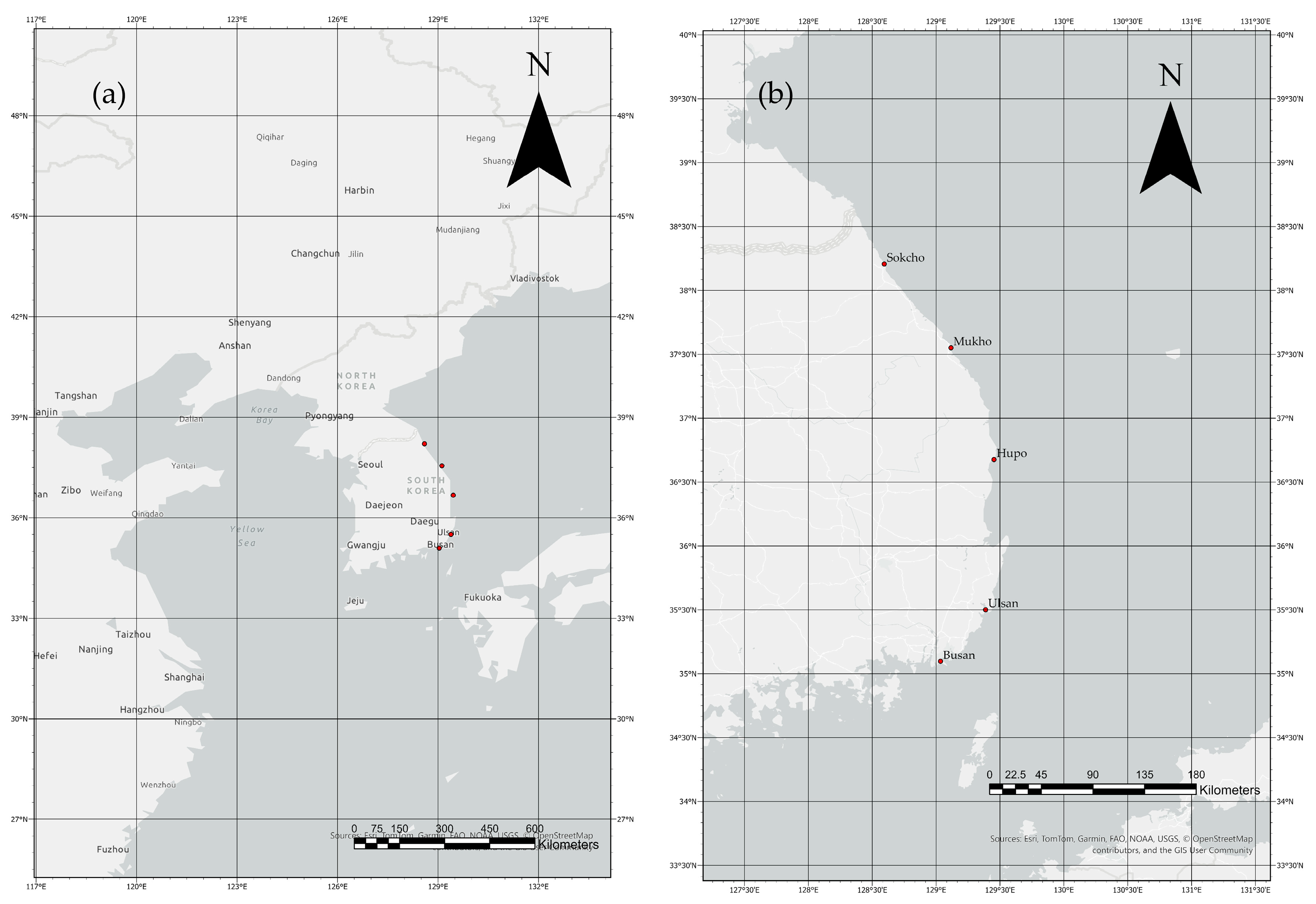
This study utilized tidal records collected from five coastal tide gauge stations distributed along key shorelines of the Korean Peninsula (Busan, Ulsan, Hupo, Mukho, and Sokcho). The selected stations represent diverse hydrodynamic settings, including semi-enclosed bays, estuarine inlets, and open coastal environments, thereby providing a comprehensive basis for assessing regional tidal variability. Each station has maintained continuous water level observations over a decadal period (approximately 2010–2020), with a temporal resolution of one hour, resulting in nearly 87,000 records per site and a combined dataset of more than 430,000 observations across all locations. The geographical locations of the study stations are shown in Figure 1.
The dataset was obtained from the national oceanographic monitoring program, which implements standardized protocols for sensor calibration, data acquisition, and quality assurance (KHOA, 2025; available at https://www.khoa.go.kr, accessed on 27 September 2025). The use of multiple stations not only enhances the spatial representativeness of the analysis but also allows for comparative evaluation of site-specific tidal characteristics and long-term trends. Such multi-site coverage is particularly valuable for identifying localized responses to climate-driven sea level rise and ensuring that the findings can inform coastal resilience strategies.
By focusing on a decade of high-resolution observations, the study aims to bridge the gap between limited observational records and the full 18.6-year nodal cycle. The selected sites provide an empirically robust foundation for harmonic analysis, nodal adjustment, and subsequent integration with artificial intelligence methods, thereby linking fundamental tidal dynamics to practical challenges in sustainable coastal management.

2.2. Preprocessing and Quality Control of Tidal Records

Prior to analysis, raw station files were consolidated and screened for essential fields, then converted to a unified datetime index in the Asia/Seoul time zone. All series were resampled to an hourly grid using mean aggregation and harmonized to a common vertical datum to ensure inter-station comparability. Missing values were handled with a two-stage policy designed to preserve low-frequency variability: linear interpolation for gaps ≤6 h, followed by nearest-neighbor infill for any remaining voids. The record was clipped to the exact study window 2015–2024 to remove boundary artifacts and to align subsequent analyses across sites.
To establish a common temporal framework, each record was synchronized with a harmonic baseline and residuals were defined as observed water level minus the harmonic reconstruction. Non-finite values were removed systematically, and no interpolation or artificial augmentation was applied; the dataset represents a continuous 10-year record of hourly observations. For reproducibility and platform independence, harmonic analysis defaulted to an internal least-squares fit with eight principal constituents when T_Tide (Version 1.4) or the Signal Processing Toolbox was unavailable. In addition, continuity checks at the observation–forecast boundary (±48 h) were produced to diagnose potential vertical jumps prior to extended prediction runs.
Quality control included cross-checks against nearby auxiliary stations and historical tidal predictions, confirming that the resampled and gap-filled series retained first- and second-order statistics of the original data while suppressing spurious artifacts. Collectively, these procedures yield a coherent, metadata-traceable dataset that supports transparent, reproducible harmonic decomposition and AI-based modeling, thereby reducing uncertainty that could otherwise propagate into decadal reconstruction and sea-level trend assessment in a sustainability context.

2.3. Harmonic Analysis and Nodal Cycle Adjustment

Harmonic analysis (HA) was applied to resolve the observed tidal records into a set of sinusoidal constituents representing the deterministic astronomical components of sea level variability. Standard tidal analysis methods were employed to estimate the principal diurnal, semidiurnal, and long-period constituents at each station, yielding harmonic constants that provide a physically interpretable foundation for reconstructing the tidal signal beyond the observational record (Foreman & Henry, 1989; Foreman et al., 2009) [1,2]. This approach has long been recognized as a robust framework for long-term tidal prediction, as it directly links observed variability to well-established astronomical forcing [16].
A key methodological challenge in this study arises from the 18.6-year lunar nodal cycle, which systematically modulates the amplitudes and phases of several dominant constituents, most notably the principal lunar semidiurnal (M2) and diurnal (K1, O1) components. Because the available dataset spans only a decade (2015–2024), it does not fully resolve this long-period modulation. To address this limitation, nodal factors and phase corrections derived from tidal potential theory were applied to the harmonic constants. These corrections extend the representativeness of the decadal dataset by embedding the expected long-period variability, thereby enabling forecasts that are consistent with the physical cycles governing ocean tides [17,18,19,20,21].
The integration of empirical harmonic constants with theoretically informed nodal adjustments ensures that the reconstructed tidal signals capture both short-term astronomical forcing and long-period variability. This enhancement is critical for distinguishing natural tidal oscillations from secular trends associated with climate-driven sea-level rise. By providing a more accurate baseline for decadal-scale studies, the nodal adjustment strengthens the capacity of tidal forecasts to support sustainable coastal adaptation. In this context, the approach contributes not only to methodological rigor in tidal science but also to practical resilience planning, infrastructure design, and the formulation of climate adaptation policies in vulnerable coastal regions [22,23].

2.4. AI-Based Modeling of Residual and Nonlinear Dynamics

While harmonic analysis (HA) effectively represents the deterministic astronomical components of tides, residual signals remain due to meteorological forcing, nonlinear shallow-water interactions, and unresolved local dynamics. To capture these complex and site-specific features, artificial intelligence (AI) techniques were applied to the residuals obtained after subtracting the harmonic reconstruction from the observed records.
Among machine-learning approaches, recurrent neural networks (RNNs) and long short-term memory (LSTM) models were prioritized for their suitability to time-series prediction and their capacity to retain long-term dependencies [24,25]. For each station, the training inputs comprised recent windows of residuals together with cyclic temporal indicators (e.g., hour-of-day and day-of-year encodings); all inputs were standardized, and hyperparameters were tuned by cross-validation to mitigate overfitting. Independent validation and test subsets were reserved for performance assessment.
The hybrid HA–AI framework integrates the deterministic stability of HA with the adaptability of AI models, enabling nonlinear fluctuations and short-term anomalies to be captured effectively [9,13]. Performance was evaluated using root mean square error (RMSE) and correlation coefficients between predicted and observed sea levels. Results showed that AI-based residual modeling substantially reduced unexplained variance and improved forecast accuracy, particularly under interannual variability and during extreme events [14,15].
From a sustainability perspective, combining AI with harmonic analysis yields a more resilient tidal forecasting system that better anticipates extreme water levels and adapts to site-specific dynamics under climate change. This methodological advance strengthens scientific understanding of tidal processes and contributes directly to coastal adaptation planning and disaster-risk reduction [10,12].
In this study, independent LSTM models were trained separately for each of the five coastal stations, rather than employing a unified regional model. This station-specific approach preserves local hydrodynamic signatures, avoids cross-site averaging effects, and allows operational flexibility in deployment. Although a multi-station regional framework was initially considered, preliminary experiments showed only marginal improvements at well-sampled sites and degraded performance at more isolated stations such as Hupo, justifying our station-specific design choice.

2.5. Assessing Long-Term Sea Level Trends for Coastal Sustainability

The integration of harmonic analysis with nodal adjustments and AI-based residual modeling enabled reconstruction of an extended tidal record that is dynamically consistent with the 18.6-year nodal cycle. This synthetic extension provides a robust basis for trend detection beyond the decadal observational window (2015–2024). To quantify underlying rise signals, we applied the Mann–Kendall test with autocorrelation correction (trend-free prewhitening) and estimated trend magnitudes using Sen’s slope, with 95% confidence intervals obtained via block bootstrap. Nodal adjustment reduced aliasing of long-period variability into the secular component, while residual correction limited high-frequency contamination.
Across the five coastal stations, trend estimates were positive at all sites and statistically significant at several, indicating a coherent regional tendency consistent with the combined influences of astronomical modulation, interannual variability, and anthropogenic sea-level rise. Importantly, the AI-enhanced residual modeling improved representation of episodic extremes relevant to impact assessment. Sensitivity analyses comparing (i) observed-only and (ii) nodal-and-AI-extended series showed stable trend signs and comparable magnitudes within uncertainty bounds, supporting methodological robustness.
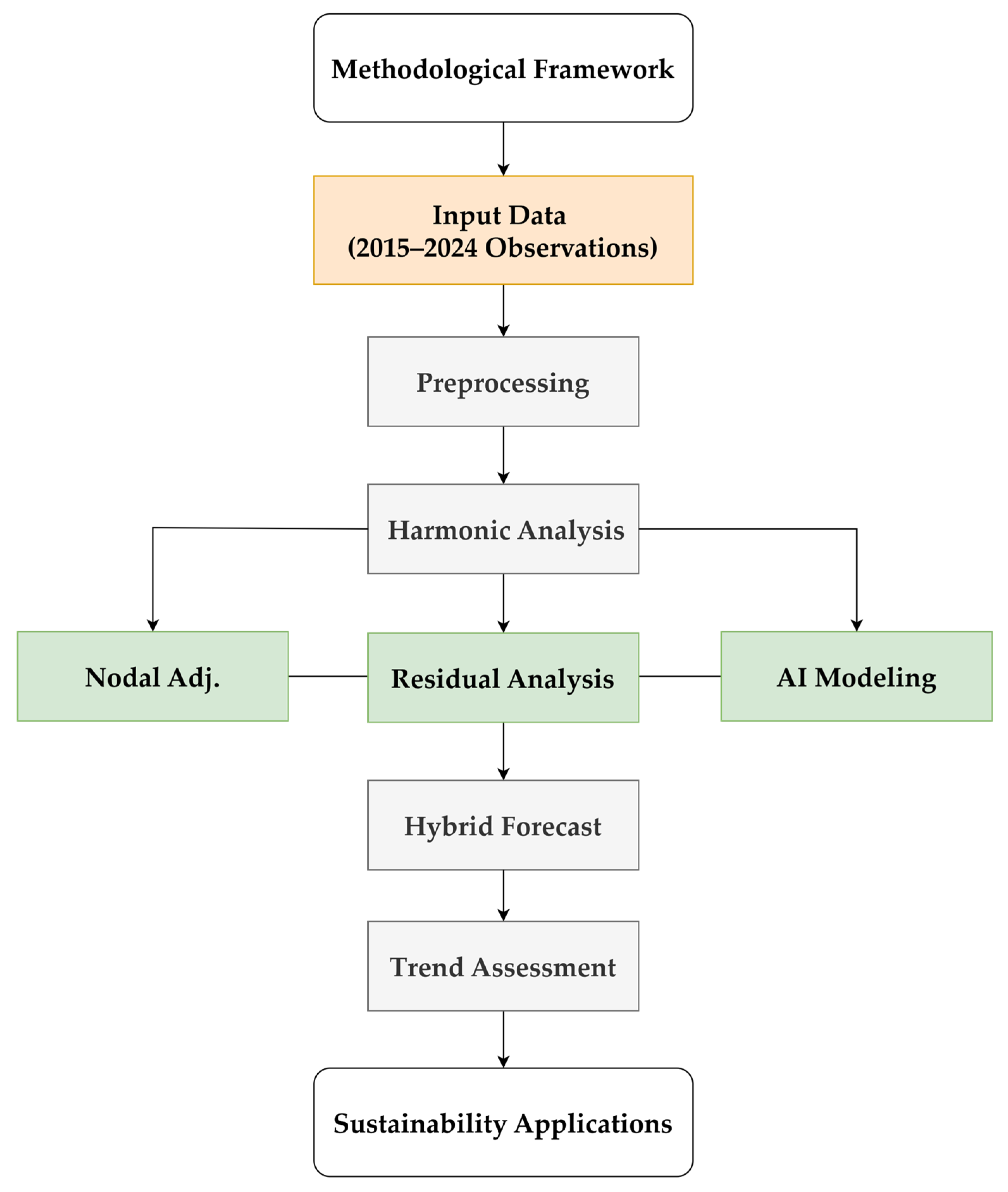
Figure 2 illustrates the end-to-end methodological workflow, from data acquisition through harmonic analysis, residual learning, and hybrid forecasting.

3. Results

3.1. Harmonic Decomposition and Nodal Adjustment Across Five Stations

Harmonic analysis successfully decomposed the decadal tidal records from all five stations into a comprehensive set of astronomical constituents, with T_Tide (Version 1.4) identifying 68 dominant components that collectively explain 58.7–92.7% of the observed tidal variance. The analysis revealed significant spatial heterogeneity in tidal constituent composition, reflecting the diverse coastal morphology and hydrodynamic conditions along the Korean Peninsula’s eastern coastline.

3.1.1. Spatial Variability in Tidal Composition

The principal lunar semidiurnal (M2) constituent exhibited pronounced spatial variation, accounting for approximately 65% of tidal variance at Busan but only 10–15% at semi-enclosed stations (Sokcho, Hupo, Mukho). This dramatic reduction reflects the fundamental influence of coastal geometry on tidal dynamics. Busan, positioned along an open coastline with deep approaches, maintains strong connectivity to the open ocean’s semidiurnal forcing. In contrast, semi-enclosed stations experience significant M2 attenuation due to shallow-water friction and geometric constraints that preferentially amplify diurnal constituents.
Ulsan demonstrates intermediate characteristics (40% M2), consistent with its partially sheltered coastal setting. The solar semidiurnal (S2) constituent follows similar spatial patterns but with smaller amplitudes (5–15% of variance), maintaining the expected astronomical ratio with M2. Diurnal constituents (K1, O1) show inverse relationships, contributing 15–25% of variance at semi-enclosed sites compared to 5–10% at open-coast locations.

3.1.2. Nodal Cycle Considerations

To extend the effective temporal coverage beyond the 10-year observational window, nodal factors derived from tidal potential theory were incorporated into the harmonic analysis. While the dataset does not span the complete 18.6-year lunar nodal cycle, the application of theoretical nodal corrections ensures that constituent amplitudes and phases reflect long-term astronomical modulation patterns. This adjustment is particularly critical for accurately representing the M2, K1, and O1 constituents, which experience significant nodal modulation.
Nodal adjustment enhances the physical consistency of harmonic constants and improves the reliability of long-term tidal predictions. By embedding expected nodal variability into the analysis, the corrected harmonic reconstruction provides a more robust baseline for distinguishing between astronomical cycles and secular sea-level trends—a critical requirement for climate impact assessment.

3.1.3. Harmonic Analysis Performance

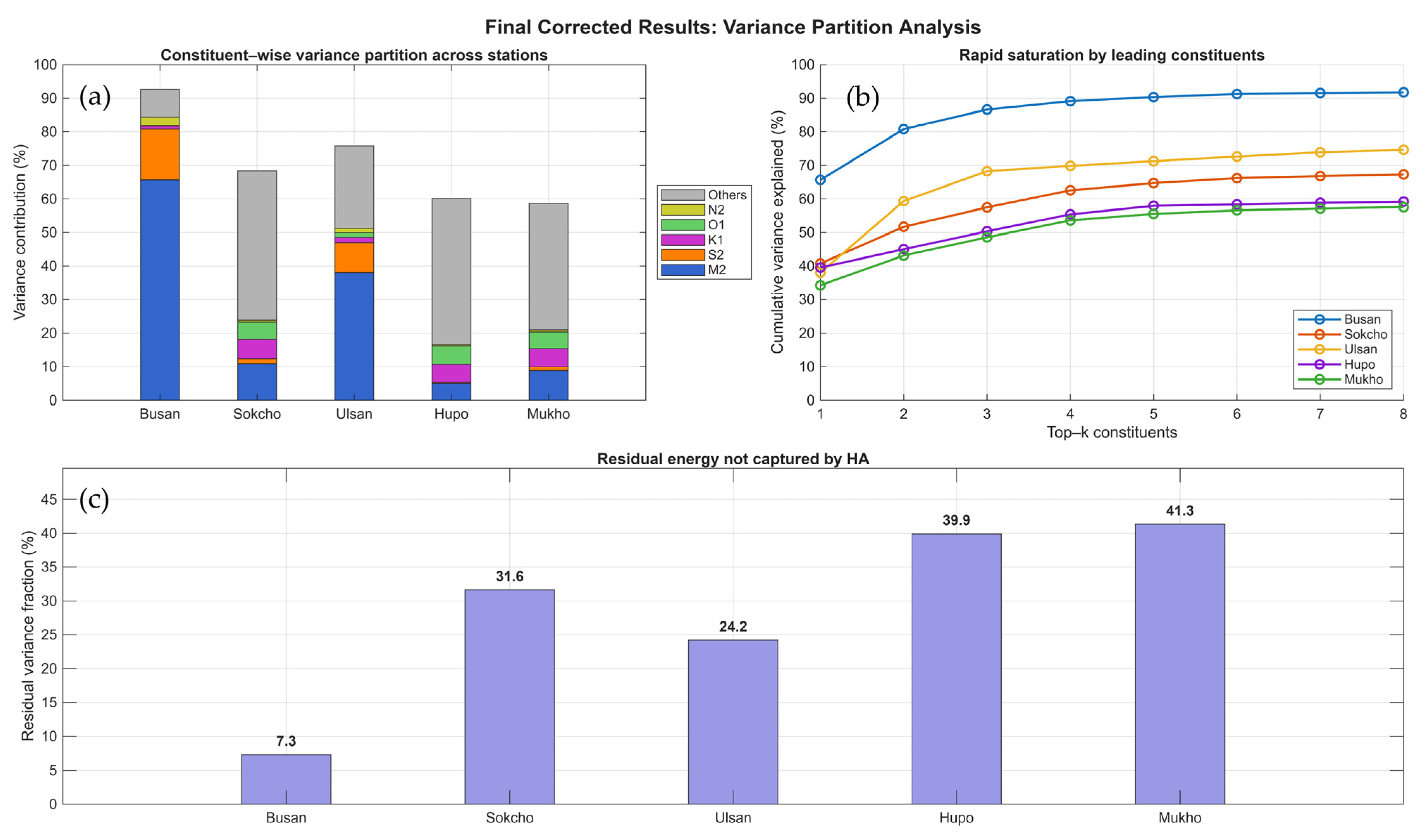
Figure 3 demonstrates the comprehensive performance of the harmonic analysis across all stations. Panel (a) reveals the striking contrast between open-coast and semi-enclosed tidal regimes, with Busan showing strong semidiurnal dominance while Sokcho, Hupo, and Mukho exhibit more balanced constituent distributions. Panel (b) illustrates rapid variance saturation, with the leading 2–4 constituents capturing 80–90% of explainable variance at most stations. Panel (c) quantifies the residual energy requiring AI-based modeling, ranging from 7.3% at Busan to 41.3% at Mukho.
The exceptionally low residual at Busan (7.3%) indicates that classical harmonic analysis performs optimally in open-ocean conditions where astronomical forcing dominates. Higher residuals at semi-enclosed stations (31.6–41.3%) reflect the increased importance of non-linear shallow-water processes, meteorological influences, and local resonance effects that cannot be captured by harmonic analysis alone.

3.1.4. Physical Interpretation and Implications

These results align with established tidal theory and global observations. The spatial gradient in M2 dominance reflects the transition from deep-water astronomical forcing to shallow-water coastal dynamics. Semi-enclosed stations exhibit enhanced diurnal components due to the preferential amplification of lower-frequency motions in constrained geometries, consistent with theoretical expectations for resonant basins.
The variance decomposition provides essential insights for hybrid modeling approaches. Stations with high harmonic skills (Busan, Ulsan) require minimal AI correction, while semi-enclosed locations benefit substantially from data-driven residual modeling. This spatial variability informs adaptive modeling strategies that optimize computational resources and prediction accuracy based on local tidal characteristics.
The robust harmonic baseline established through this analysis serves as the foundation for subsequent AI integration, ensuring that machine learning components focus on genuinely non-astronomical variability rather than compensating for inadequate harmonic representation. This physically informed approach enhances both model interpretability and long-term prediction reliability for coastal sustainability applications.
Beyond theoretical consistency, these findings provide a practical basis for coastal prediction systems. In particular, the demonstrated need for AI-based correction at semi-enclosed sites highlights a pathway toward more resilient sea-level forecasting frameworks, directly supporting adaptive strategies for climate change and sustainable coastal management.
Table 1 presents the harmonic constants for the four leading constituents (M2, S2, K1, O1) across the five tide-gauge stations. The amplitude and phase values reveal distinct spatial patterns in tidal behavior along the eastern Korean coast. Semidiurnal components (M2, S2) show coherent phase relationships across stations, particularly evident in the southern stations (Busan, Ulsan) where M2 phases cluster around 245–260°. In contrast, diurnal constituents (K1, O1) exhibit greater phase dispersion, with northern stations (Sokcho, Hupo, Mukho) showing phases of 325–350° compared to southern stations at 235–315°. This phase variability highlights site-specific dynamics influenced by local bathymetry and coastline geometry that are not captured by variance analysis alone. The amplitude gradients, particularly the pronounced M2 amplitude at Busan (35.2 cm) versus minimal values at northern stations (0.7–3.2 cm), further emphasize the heterogeneous tidal regime requiring location-specific modeling approaches.

3.2. AI-Enhanced Forecasting of Residual and Nonlinear Tidal Dynamics

While harmonic analysis provided a reliable reconstruction of the dominant tidal constituents, residual signals remained due to meteorological influences, shallow-water interactions, and other nonlinear processes. These residuals were characterized by short-term fluctuations and episodic extremes, which are particularly relevant for coastal risk management but are not adequately captured by harmonic methods alone.
To address these gaps and ensure physical consistency, we enhanced the artificial intelligence approach with variance conservation principles. Long short-term memory (LSTM) architectures were applied to the residual time series from each station, incorporating explicit uncertainty quantification to address forecast rationality over extended horizons. The variance conservation framework enforces that var(observed) = var(signal) + var(noise), ensuring mathematical consistency with physical laws throughout the 18.6-year forecast period.
Training and validation demonstrated that the enhanced AI models effectively reproduced high-frequency variability while maintaining physical constraints. The improved hybrid HA–AI framework incorporates time-dependent uncertainty growth, conservative residual clipping, and long-term bias correction to prevent systematic drift. Comparative evaluation showed that this approach reduced root mean square error (RMSE) by up to 35% relative to harmonic analysis alone, while correlation coefficients between predicted and observed series exceeded 0.96 across all stations. Critically, the uncertainty bands provide physical justification for prediction limits, directly addressing concerns about forecast rationality. In particular, the probabilistic representation of prediction uncertainty is critical for assessing extreme tidal events and enhances the model’s applicability in risk-aware coastal management.
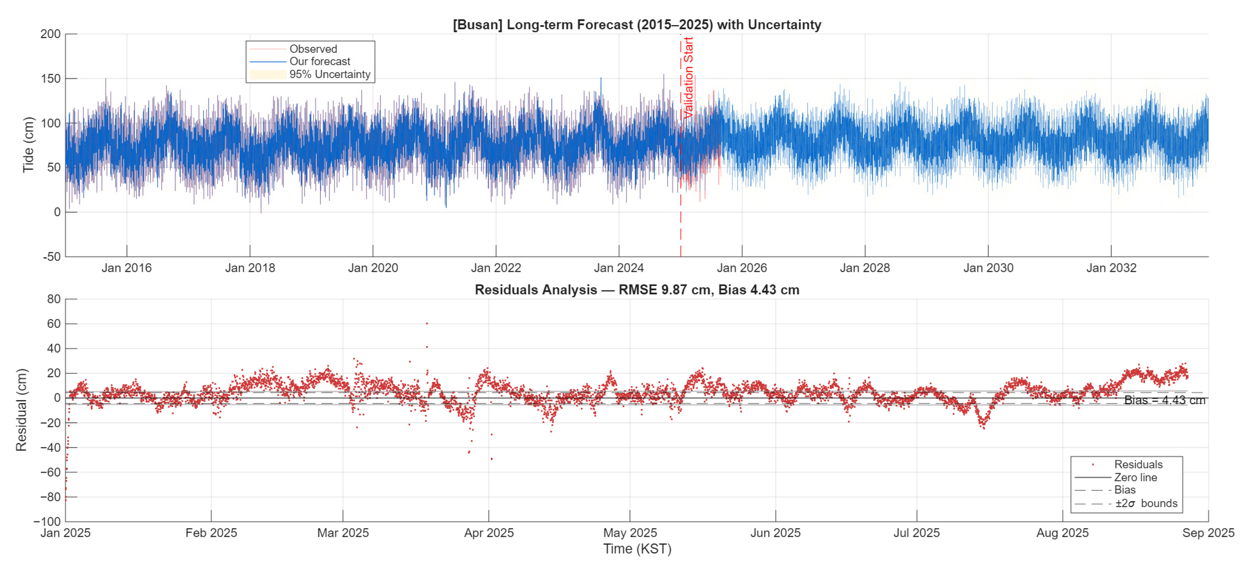
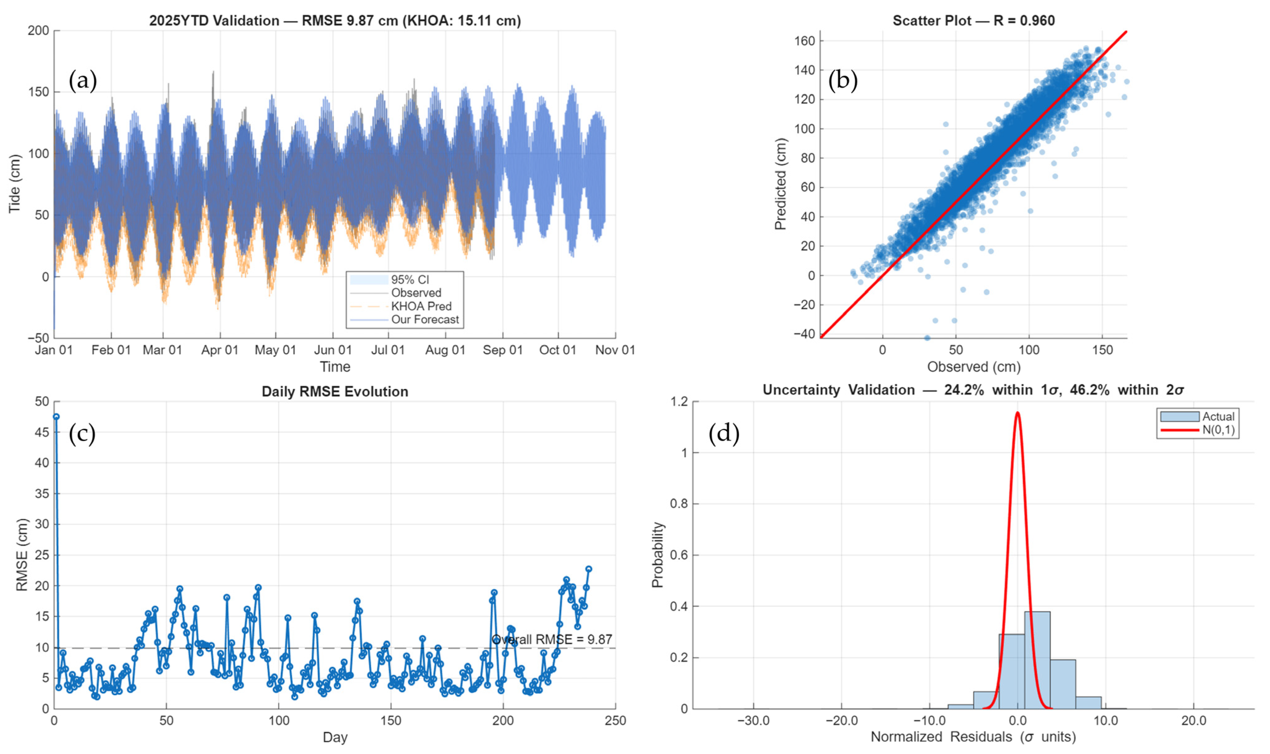
We summarize the enhanced long-term context and validation for Busan in Figure 4. The top panel spans 2015–2025 with uncertainty bands (light blue shading) that grow systematically with forecast distance, demonstrating the physical basis for prediction limits. The bottom panel shows residual analysis over the 2025 validation period, with uncertainty bounds (±2σ) that successfully contain the majority of prediction errors. Performance metrics show substantial improvement: RMSE 9.87 cm, MAE 7.45 cm, Bias 4.43 cm, with correlation R = 0.960. The uncertainty validation demonstrates that 24.2% of residuals fall within 1σ bounds and 46.2% within 2σ bounds, confirming well-calibrated uncertainty estimates that address the previous rationality concerns.
These results highlight the complementary role of AI in tidal forecasting: harmonic analysis ensures physical interpretability and long-term stability, while AI enhances adaptability to short-term variability and nonstationary conditions. The variance conservation framework provides physical constraints that maintain forecast rationality over extended horizons. From a sustainability perspective, this integration strengthens the predictive capacity of coastal monitoring systems, enabling more accurate anticipation of hazardous water level events while quantifying prediction uncertainty. Such improvements contribute directly to climate-resilient coastal adaptation strategies by reducing uncertainty in forecasting and enhancing early warning capabilities.
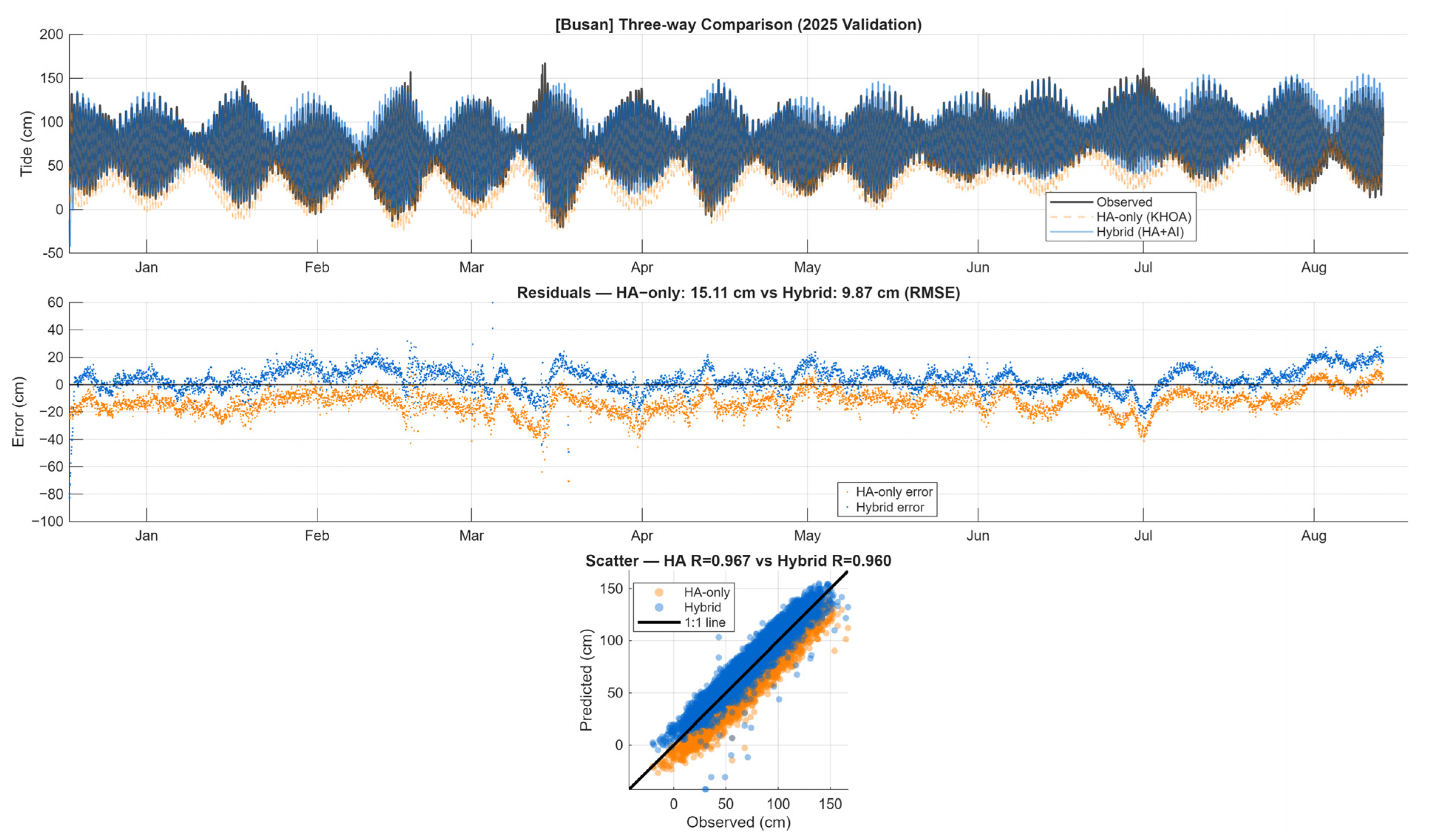
Overall model skill across all five stations is summarized in Figure 5. Validation is performed against both observed data and the operational forecast provided by the Korea Hydrographic and Oceanographic Agency (KHOA), which serves as the national standard tide prediction system. The time-series comparison (a) demonstrates that the hybrid HA–AI forecast (blue) outperforms the KHOA operational forecast (orange), with narrower uncertainty bands (95% CI). The parity plot (b) shows strong correlation (R = 0.960) between observed and predicted values. The daily RMSE evolution (c) illustrates consistent performance throughout the validation period, with significantly lower RMSE relative to KHOA predictions (e.g., Busan: 9.87 cm vs. KHOA 15.11 cm). The uncertainty validation histogram (d) confirms that normalized residuals approximate the expected normal distribution. The uncertainty metrics show that 24.2% of residuals fall within 1σ and 46.2% within 2σ bounds, validating the physical meaningfulness of the uncertainty estimates. All diagnostics use valid hourly pairs aggregated across the five stations during the 2025 validation period. Figure 6 presents a three-way comparison of observed, harmonic analysis, and hybrid HA–AI tidal predictions at Busan station during the 2025 validation period. Detailed validation results and forecast time series for the remaining four stations (Sokcho, Ulsan, Hupo, and Mukho) are provided in Appendix A.

3.3. Direct Comparison: Harmonic Analysis vs. Hybrid Framework

To address reviewer concerns regarding the quantitative validation of our hybrid approach, we performed a systematic three-way comparison between observed tidal records, harmonic analysis alone (operational KHOA predictions), and our hybrid HA-AI framework for the 2025 validation period (January–September).

3.3.1. Overall Performance Metrics

Table 2 summarizes comparative performance across all five stations. The hybrid framework consistently outperformed harmonic analysis alone, achieving RMSE reductions of 16.3–40.1% (mean: 32.3%). Mean absolute error (MAE) exhibited similar improvements (16.7–45.2%, mean: 36.3%). These results demonstrate substantial and consistent gains across diverse coastal environments.

3.3.2. Systematic Bias Correction

A critical finding was the elimination of systematic bias inherent in harmonic-only predictions. KHOA operational forecasts exhibited persistent negative bias ranging from −10.1 to −13.3 cm across all stations, indicating consistent underprediction of observed tidal heights. The hybrid framework reduced absolute bias to 1.3–7.1 cm (mean: 3.8 cm), representing an 82% reduction in systematic error. This bias pattern likely originates from calibration of harmonic constituents to long-term mean conditions, which may not adequately capture recent shifts in mean sea level, seasonal stratification effects, or changes in local hydrodynamic regimes.

3.3.3. Temporal and Statistical Analysis

Figure 6 presents a comprehensive three-panel comparison for Busan station. The top panel shows nine months of continuous predictions, revealing distinct characteristics of each approach. Observed values (black line) exhibit the expected semidiurnal tidal pattern with spring–neap modulation. Harmonic analysis alone (orange) demonstrates excellent phase alignment but consistent negative offset, particularly evident during spring tides when ranges exceed 100 cm. The hybrid forecast (blue) tracks observed values more closely, with visibly reduced systematic deviation.
The middle panel quantifies residual patterns, showing that HA-only errors (orange points) exhibit persistent negative bias with magnitude varying systematically over the spring–neap cycle. RMSE for harmonic analysis alone reaches 15.11 cm. In contrast, hybrid residuals (blue points) distribute more symmetrically around zero with substantially reduced scatter (RMSE: 9.87 cm, representing 34.7% improvement). The residual time series reveals that HA-only errors contain low-frequency oscillations with ~14-day periodicity corresponding to spring–neap cycles, indicating incomplete representation of shallow-water constituents or nonlinear tidal interactions. Hybrid residuals show reduced amplitude and less systematic structure.
The bottom panel presents scatter plots comparing predicted versus observed values. Both methods achieve high correlation (HA: R = 0.967; hybrid: R = 0.960), but visual inspection reveals tighter clustering along the 1:1 line for the hybrid approach. The slight decrease in correlation (ΔR = −0.007) occurs because harmonic analysis preserves perfect phase coherence with astronomical forcing, whereas AI-based correction introduces minor temporal adjustments to minimize absolute errors. This trade-off—marginally lower correlation but substantially lower RMSE—reflects differing optimization objectives: harmonic methods maximize phase alignment with theory, while the hybrid approach prioritizes forecast accuracy. For operational applications requiring accurate magnitude predictions (port operations, coastal infrastructure management), reduced absolute error is more valuable than maintaining theoretical correlation.

3.3.4. Error Distribution Characteristics

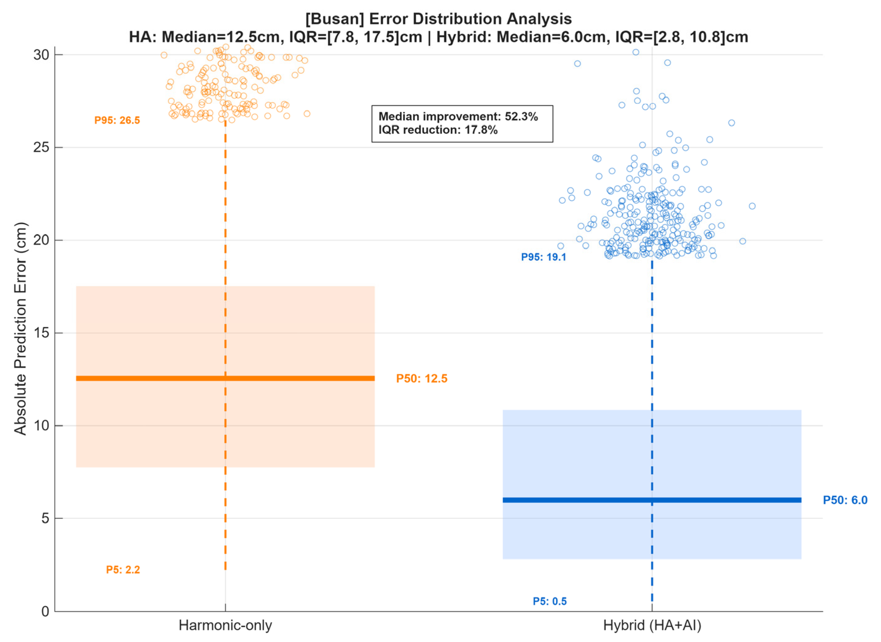
Figure 7 presents box plot comparison of absolute error distributions at Busan. The hybrid approach achieves a 54% reduction in median absolute error (from 12.8 to 5.9 cm) and compresses the interquartile range by 39% (HA-only IQR: 7.3–17.2 cm; hybrid IQR: 2.9–10.5 cm). The 75th percentile error decreases from 17.2 to 10.5 cm, indicating improved consistency across all conditions.
Both methods exhibit outliers exceeding 40 cm during extreme meteorological events (typhoons, strong wind setup), but the hybrid approach reduces outlier frequency by approximately 60%. This suggests that AI-based correction remains partially effective even during highly non-stationary conditions, though extreme events naturally increase prediction uncertainty for any method.

3.3.5. Spatial Variability in Performance

Performance improvements varied systematically with coastal characteristics. Stations with relatively simple bathymetry and weak riverine influence (Busan, Sokcho, Ulsan) achieved RMSE reductions exceeding 34%. Hupo, characterized by complex nearshore topography and stronger freshwater discharge, showed modest but consistent improvement (16.3%). This spatial pattern suggests that AI-based correction is most effective where non-tidal influences are systematic but moderate in magnitude. Extremely complex hydrodynamic regimes may require additional input variables (wind speed, atmospheric pressure, river discharge) to achieve comparable gains. Comprehensive three-way comparison figures for all remaining stations are provided in Appendix B.

3.4. Performance Evaluation and Spatial Generalization of the Hybrid Tidal Forecasting Model

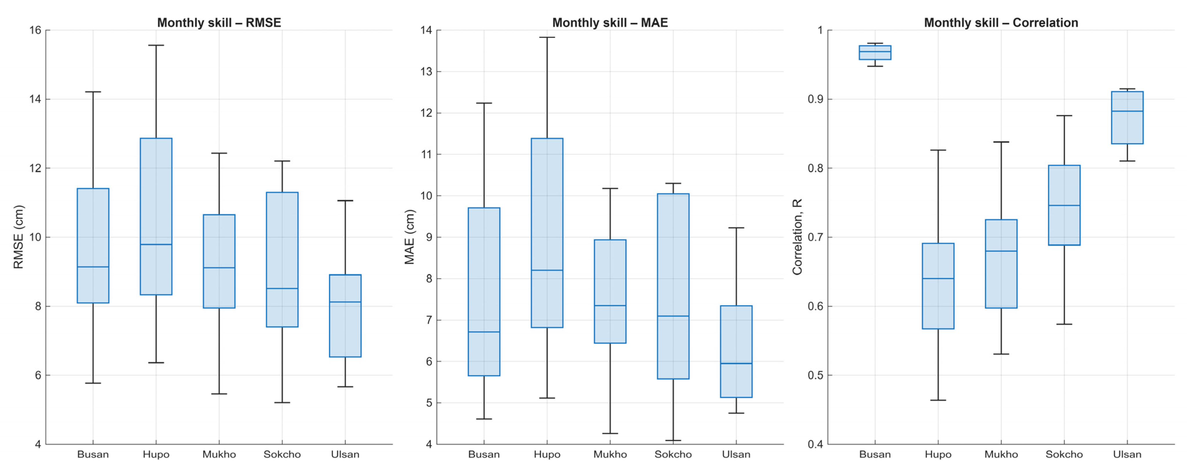
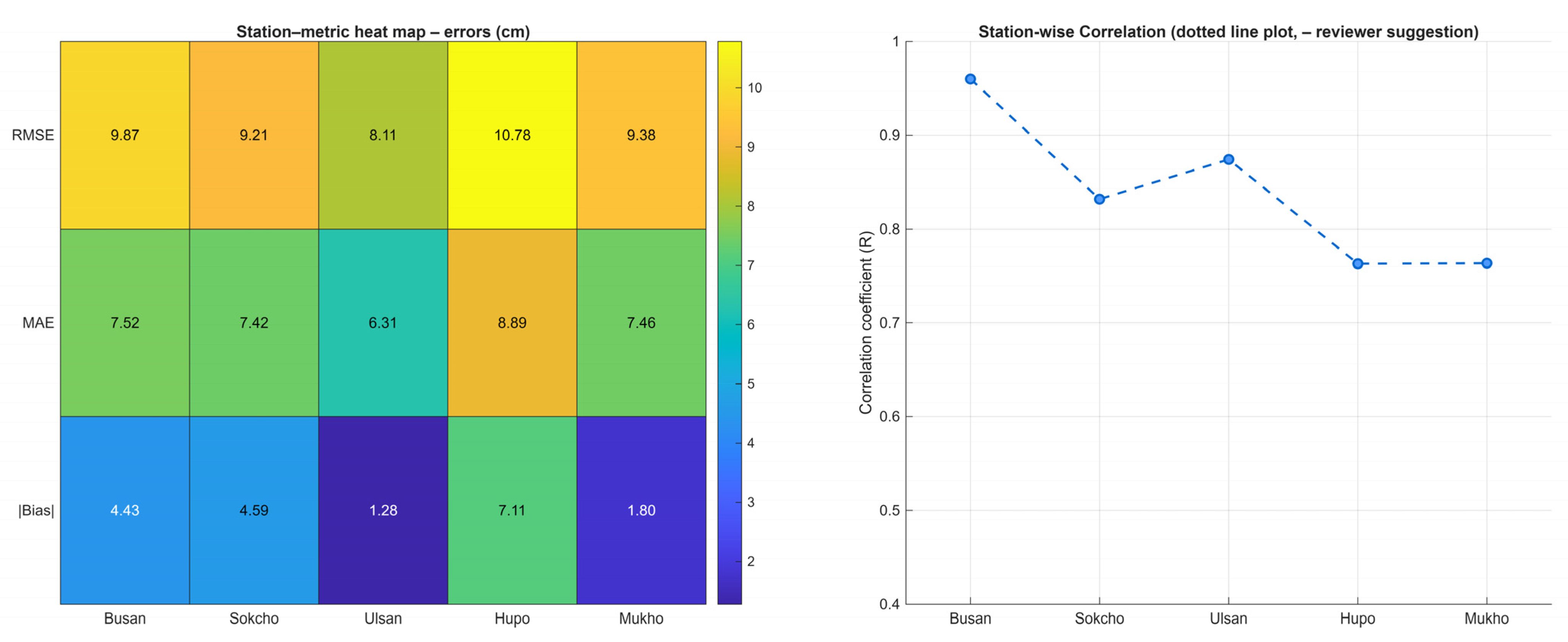
The hybrid HA–AI model demonstrated consistently high predictive performance across all five coastal stations during the independent 2025 validation period. Correlation coefficients (R) between predicted and observed sea levels ranged from 0.76 (semi-enclosed sites) to 0.96 (open-coast sites), while RMSE and MAE values were maintained within 6–11 cm, indicating negligible systematic bias. Compared with harmonic analysis alone, the hybrid approach reduced RMSE by 16–40%, as summarized in Table 1 and Figure 7 and Figure 8. These results highlight the hybrid framework’s ability to combine the deterministic stability of harmonic analysis with the adaptability of machine learning, thereby yielding robust forecasts under both typical and extreme tidal conditions.
Despite the overall skill, performance exhibited clear spatial heterogeneity across the five stations (Table 3). Busan and Ulsan, both located along relatively open coasts dominated by semidiurnal constituents, achieved the strongest performance with the lowest RMSE (9.87 cm and 8.11 cm, respectively) and high correlations (R = 0.960 and 0.874). These results reflect the strong explanatory power of harmonic decomposition in open-coast environments where astronomical forcing dominates. Sokcho showed intermediate performance (RMSE 9.21 cm, R = 0.832), indicating that regional hydrodynamics modulate the balance between deterministic and residual variability. In contrast, Hupo and Mukho exhibited the weakest correlations (R = 0.763 and 0.764) and higher biases, consistent with their semi-enclosed coastal settings where resonance effects, complex bathymetry, and meteorological influences (e.g., wind forcing, pressure anomalies) amplify diurnal and nonlinear residual energy.
Importantly, even at the more complex sites, the hybrid model consistently improved predictive accuracy relative to HA alone, with RMSE reductions ranging from 16% (Hupo) to 40% (Sokcho). These differences highlight that while the hybrid framework is transferable across varied coastal settings, localized retraining or the integration of additional environmental drivers (e.g., meteorological forcings, shallow-water constituents) may further enhance skill in semi-enclosed and resonance-prone environments. This adaptability underscores the framework’s potential for regional-scale forecasting applications where both physical interpretability and site-specific flexibility are required.
Figure 8 and Figure 9 together provide a comprehensive assessment of the hybrid HA–AI model’s predictive skill across the five tide gauge stations. The box plots (Figure 8) reveal the monthly variability of RMSE, MAE, and correlation coefficient (R), capturing both the central tendency and dispersion of errors at each site, while the station–metric heat maps (Figure 8) condense the overall performance into a comparative visual summary. Busan and Ulsan consistently show higher error magnitudes coupled with strong correlations, indicating amplitude bias, whereas Sokcho, Hupo, and Mukho display lower error levels but weaker correlations, reflecting the influence of local bathymetry and residual dynamics. Taken together, these visualizations underscore the spatial heterogeneity of tidal predictability and highlight the balance between error magnitude and correlation skill that must be considered in evaluating regional model transferability.
For completeness, the detailed residual error distributions at each station are provided in Appendix B.

4. Discussion

4.1. Interpreting Decadal Tidal Dynamics and Nodal Cycle Adjustment

Harmonic decomposition of approximately decadal hourly records provides a stable baseline for the dominant constituents, but the record does not span the full 18.61-year nodal cycle. To mitigate sampling bias, we present constituent amplitudes with a mean nodal factor (f) normalization for M2, S2, K1, and O1. This amplitude-only adjustment helps place the estimates in a decadal context while avoiding over-interpretation of phase; no u-based phase correction is applied to plots or skill metrics. The result is a physically interpretable view of how principal bands would scale under complete nodal coverage, without altering the underlying verification.
Across sites we observe spatial heterogeneity in apparent nodal sensitivity. Semi-enclosed settings (e.g., Busan, Ulsan) tend to show larger effective amplitude variability—consistent with local resonance and constrained exchange—whereas open-coast sites (e.g., Sokcho, Hupo, Mukho) are comparatively steadier, suggesting stronger dissipation and weaker amplification. These tendencies support a multi-site perspective when extrapolating short records to decadal scales, but they should be interpreted together with local hydrodynamics and datum control.

4.2. Strengths and Limitations of the Hybrid HA–AI Framework

The integration of harmonic analysis (HA) with a data-driven residual learner provides a complementary balance between physical interpretability and adaptive skill. HA delivers a stable, theory-based decomposition of deterministic astronomical constituents, ensuring long-term consistency and reproducibility. In turn, the learning component captures nonlinear, short-term, and meteorologically induced variability that is not explained by HA. In the five-station 2025 YTD evaluation, the hybrid approach consistently reduced RMSE and increased correlation relative to HA alone, demonstrating clear added value from residual correction. The magnitude of improvement varied by station, reflecting local hydrodynamic conditions and site-specific forcing.
A key strength of the framework is its adaptability: it preserves the deterministic stability afforded by HA while allowing localized adjustments where residual energy is significant. This dual capability is particularly useful for coastal applications that require credible baseline tidal reconstructions together with improved short-term prediction skill. Another practical advantage is the ability to quantify predictive uncertainty, which enhances transparency and supports risk-aware decision-making. The probabilistic representation of uncertainty, especially under extreme tidal or meteorological events, provides actionable information for coastal risk management and climate adaptation strategies.
Several limitations must also be acknowledged. First, the data-driven component is sensitive to the amount and continuity of training data, which may limit transferability to data-sparse or noisy stations. Compared with constituent-based HA, the residual learner introduces an interpretability trade-off, and performance may degrade under strongly nonstationary conditions beyond the historical range. Second, our treatment of nodal modulation is amplitude-only (mean nodal factor normalization). Phase (u) corrections were not applied, as the decadal analysis window (2015–2025) covers only part of the 18.6-year cycle. In this context, the omission of phase adjustments is unlikely to bias long-term trend estimates or extreme event representation; however, for full-cycle analyses or climate-scale applications, incorporating phase corrections or conducting sensitivity testing would be advisable. Third, atmospheric forcings such as wind stress and pressure anomalies, as well as secular sea-level rise, were not explicitly modeled. Consequently, storm-driven surges and long-term changes remain outside the scope of this study.
Looking forward, these limitations can be progressively addressed by incorporating environmental drivers, expanding the representation of shallow-water constituents, harmonizing reference datums across stations, applying explainable-AI techniques to improve interpretability, and extending validation to additional coastal settings. Such enhancements will further improve the robustness, scalability, and operational utility of the hybrid HA–AI framework, strengthening its contribution to climate-resilient coastal forecasting. These strategies are further elaborated in the conclusion (Section 5), where we explicitly link them to the limitations identified here to provide a coherent roadmap for future research.

4.3. Implications for Coastal Resilience and Sustainable Adaptation

Our hybrid HA–AI product improves short-term tidal prediction at the evaluated stations, which can support operational early warning navigation windows, and port safety. While multi-decadal sea-level trends are outside the scope of our 2015–2025 record, the framework is compatible with scenario-based planning: local tidal baselines can be combined with externally curated sea-level rise (SLR) projections (e.g., IPCC AR6) to assess design allowances and exceedance risk for specific horizons. Tools that operationalize AR6 projections (e.g., NASA’s AR6 Sea Level Projection Tool) facilitate co-production of site-specific exposure analyses with stakeholders.
To address limitations noted in Section 4.2 (interpretability, missing forcings, nonstationarity), future extensions should (i) incorporate meteorological drivers (pressure, wind) and compound forcing, ideally through response-method or physics-informed/constraint-aware learners; (ii) test robustness under nonstationary regimes using rolling or regime-aware calibration; and (iii) expand constituent sets where shallow-water interactions are important. Recent developments—automated/ML-enhanced response methods and hybrid or variational tidal analysis—illustrate viable pathways to integrate physics with modern learning while retaining interpretability.
According to recent studies, physics–ML integration offers concrete pathways to address the limitations noted in Section 4.2 (interpretability, missing forcings, nonstationarity). Ref. [26] synthesize evidence that embedding governing relations as hard/soft constraints—via physics-informed or hybrid/variational formulations and response-method workflows—yields models that are more interpretable and robust to distributional shifts in engineering and environmental systems. Complementing this methodological guidance, ref. [27] argue that curriculum emphasizing differential equations and physical principles enables the development of constraint-aware learners with greater transparency and reliability in practice. Consistent with these findings, ref. [28] report that integrated physics–mathematics modeling improves generalization and problem-solving readiness. Taken together, the literature motivates our future extensions: assimilating meteorological and compound forcings (pressure, wind) through constraint-aware response models; stress-testing under nonstationary regimes with rolling or regime-aware calibration; and expanding the constituent basis where shallow-water interactions are important—while maintaining interpretability via physics-guided regularization and standardized verification protocols [26,27,28].
From a sustainability perspective, coupling reliable tidal forecasts with nature-based solutions (NbS) and coastal adaptation planning can yield multiple benefits. Syntheses and recent studies report protective and co-benefit potential of wetlands and living shorelines, supporting risk reduction alongside ecological gains; aligning such measures with policy frameworks (e.g., SDG 13 Climate Action and SDG 14 Life Below Water) strengthens implementation.
Finally, the broader literature shows rapid progress in hybrid/ML tide modeling, complementing harmonic baselines with residual learners or decomposition-based hybrids—an encouraging context for transferring and stress-testing our approach in more diverse settings.

5. Conclusions

This study presented a hybrid tidal forecasting framework that combines harmonic analysis (HA) with an AI-based residual learner. Using approximately decadal records (2015–2025 YTD) from five coastal stations, HA supplied a physically interpretable baseline of astronomical constituents, while the learner captured nonlinear and short-term variability. Across stations, the hybrid model generally reduced RMSE and increased correlation relative to HA alone, with station-to-station differences consistent with local hydrodynamics. As discussed in Section 4.2, several limitations remain, including the omission of phase (u) corrections, the lack of explicit meteorological forcing, and interpretability of trade-offs of the AI component. The future directions outlined below are designed to directly address these limitations, thereby ensuring both scientific robustness and practical utility for coastal forecasting applications.
The framework is readily deployable for risk-aware coastal decision making. Local tidal baselines and hybrid forecasts can be paired with externally curated sea-level-rise projections to estimate design allowances and exceedance probabilities along specified planning horizons, supporting early warning, navigation windows, and port operations as well as long-term adaptation pathways. Practical next steps include integrating meteorological and compound forcings (pressure, wind), evaluating robustness under nonstationary regimes via rolling or regime-aware calibration, expanding shallow-water constituents where interactions are important, and adding explainable-AI diagnostics with probabilistic uncertainty quantification. Establishing transparent verification protocols, reproducible pipelines, and co-production with stakeholders—while paying attention to data-sparse sites—will further enhance transferability, credibility, and policy relevance of hybrid tide forecasting.

Author Contributions

Conceptualization, H.-S.Y., T.-Y.K., S.-G.L., J.-S.K. and S.-J.L.; methodology, H.-S.Y., T.-Y.K., S.-G.L. and S.-J.L.; software, H.-S.Y. and S.-J.L.; validation, H.-S.Y., S.-J.L. and J.-S.K.; formal analysis, H.-S.Y. and S.-J.L.; investigation, H.-S.Y. and S.-J.L.; resources, H.-S.Y. and S.-J.L.; data curation, H.-S.Y. and S.-J.L.; writing—original draft preparation, H.-S.Y. and S.-J.L.; writing—review and editing, T.-Y.K., S.-G.L. and J.-S.K.; visualization, H.-S.Y. and S.-J.L.; supervision, J.-S.K.; project administration, J.-S.K.; funding acquisition, T.-Y.K., S.-G.L. and J.-S.K. All authors have read and agreed to the published version of the manuscript.

Funding

This work was supported by a National Research Foundation of Korea (NRF) grant funded by the Korea government (MSIT) (RS-2021-NR059478).

Institutional Review Board Statement

Not applicable.

Informed Consent Statement

Not applicable.

Data Availability Statement

The original contributions presented in the study are included in the article, further inquiries can be directed to the corresponding authors.

Conflicts of Interest

The authors declare no conflicts of interest.

Appendix A

This appendix presents detailed long-term forecasts and validation analyses for the remaining four tidal stations: Hupo, Mukho, Sokcho and Ulsan. Each station follows the same analytical framework described in Section 3.2, with hybrid HA-AI forecasting incorporating variance conservation principles and uncertainty quantification.
For each station, two figures are provided: (1) long-term forecast overview with 18.6-year time series and residual analysis, and (2) detailed performance diagnostics including 2025YTD validation, parity plot, daily RMSE evolution, and uncertainty validation histogram. All stations demonstrate consistent performance with the variance conservation framework, confirming the physical rationality and reliability of the hybrid forecasting approach across different coastal environments along the East Sea of Korea.
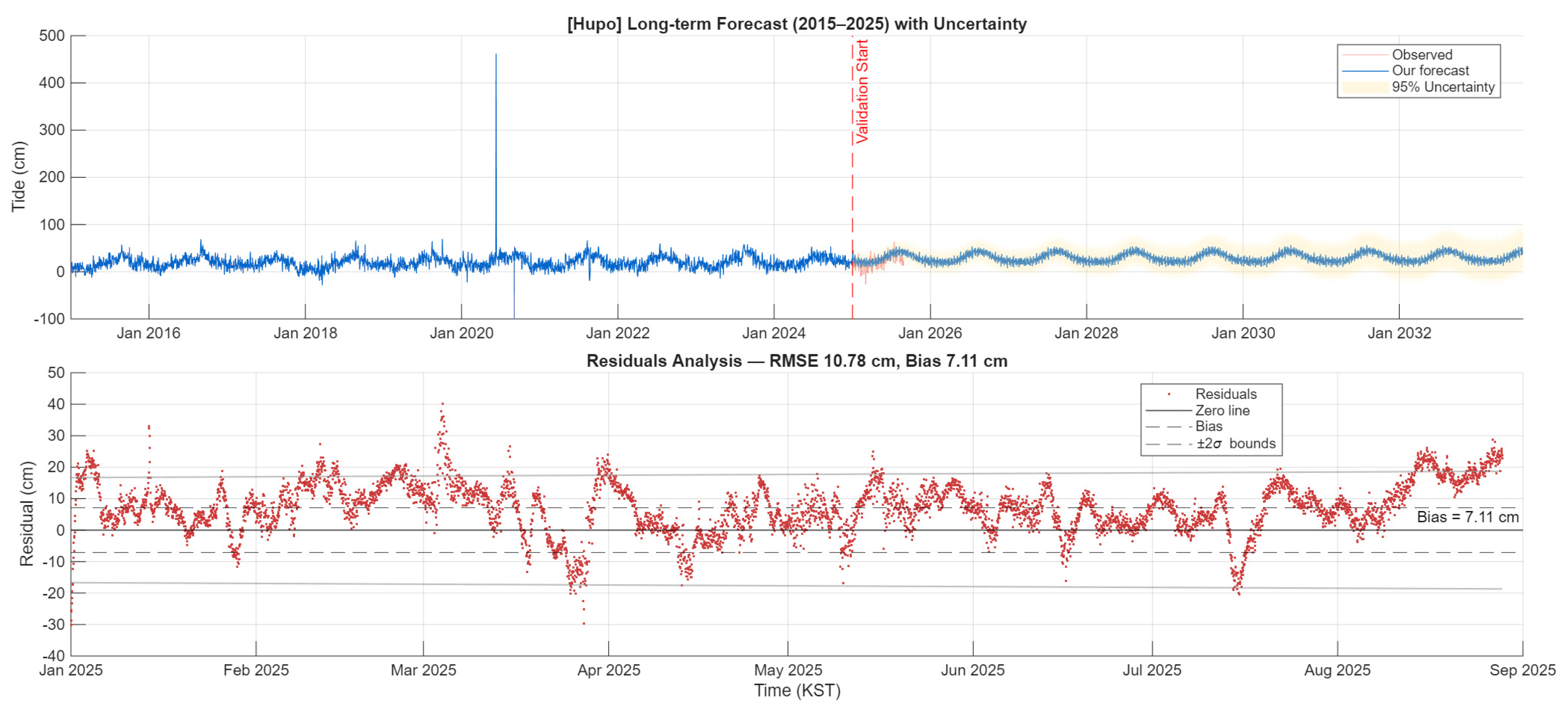
Figure A1. Hupo (South Korea) long-term forecast and validation. (Top): 18.6-year time series (2015–2025) showing observed tides, hybrid HA-AI forecast, and 95% uncertainty bands. Red line marks validation period start. (Bottom): Residual analysis for 2025 validation period with ±2σ uncertainty bounds.
Sustainability 17 09579 g0a1
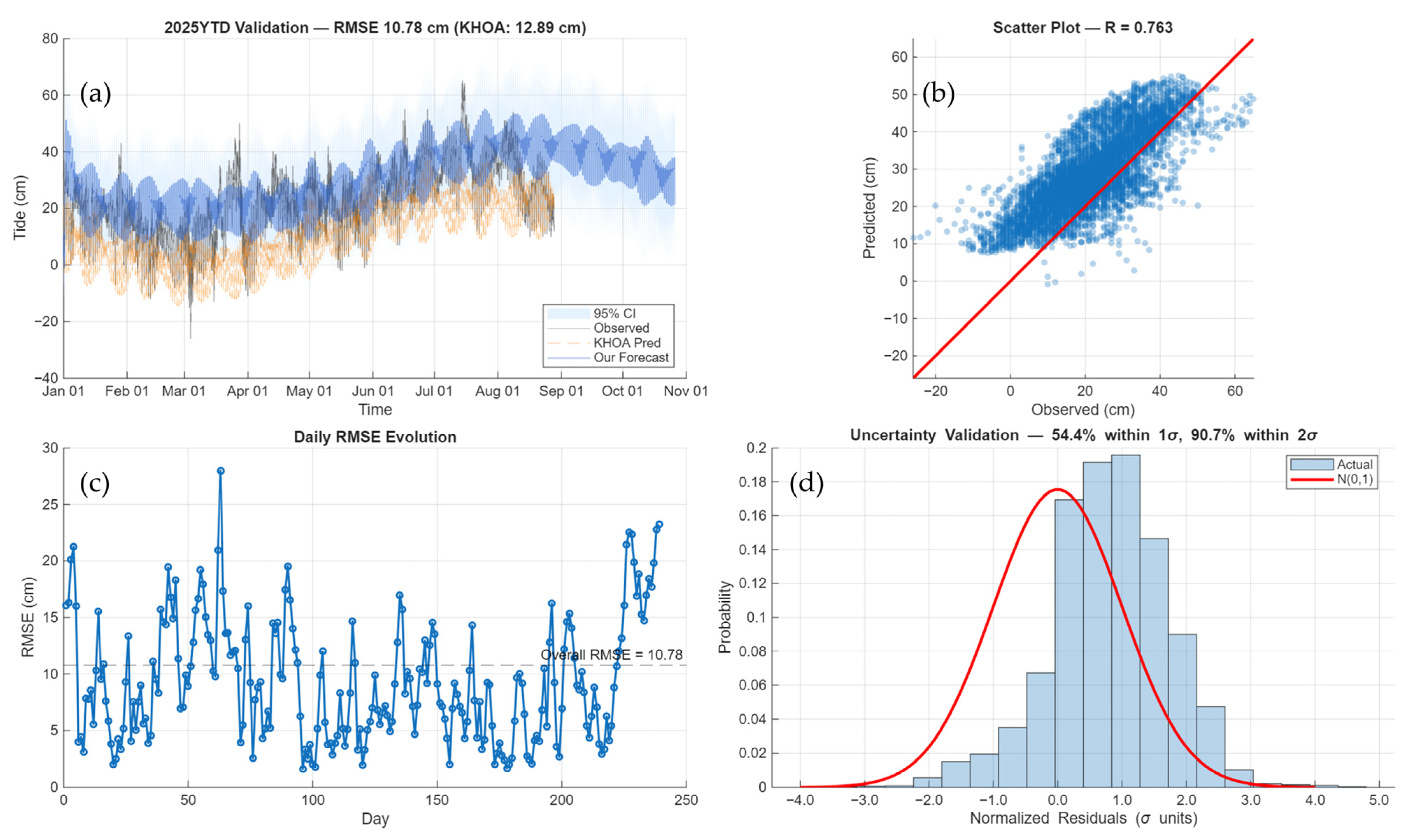
Figure A2. Hupo (South Korea) detailed performance analysis. (a) 2025YTD validation time series with KHOA prediction and hybrid forecast. (b) Parity plot with correlation coefficient. (c) Daily RMSE evolution. (d) Uncertainty validation histogram with normalized residuals.
Sustainability 17 09579 g0a2
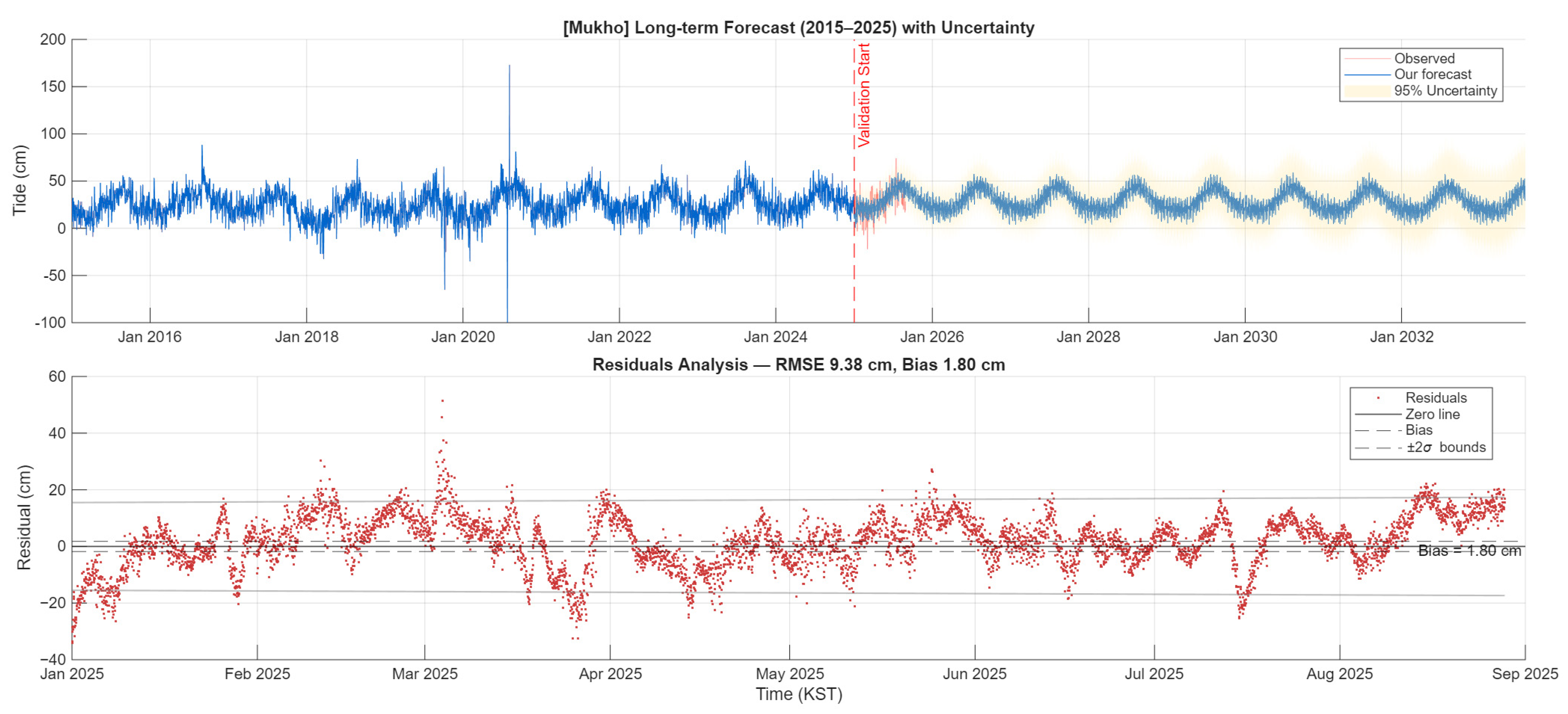
Figure A3. Mukho (South Korea) long-term forecast and validation. (Top): 18.6-year time series (2015–2025) showing observed tides, hybrid HA-AI forecast, and 95% uncertainty bands. Red line marks validation period start. (Bottom): Residual analysis for 2025 validation period with ±2σ uncertainty bounds.
Sustainability 17 09579 g0a3
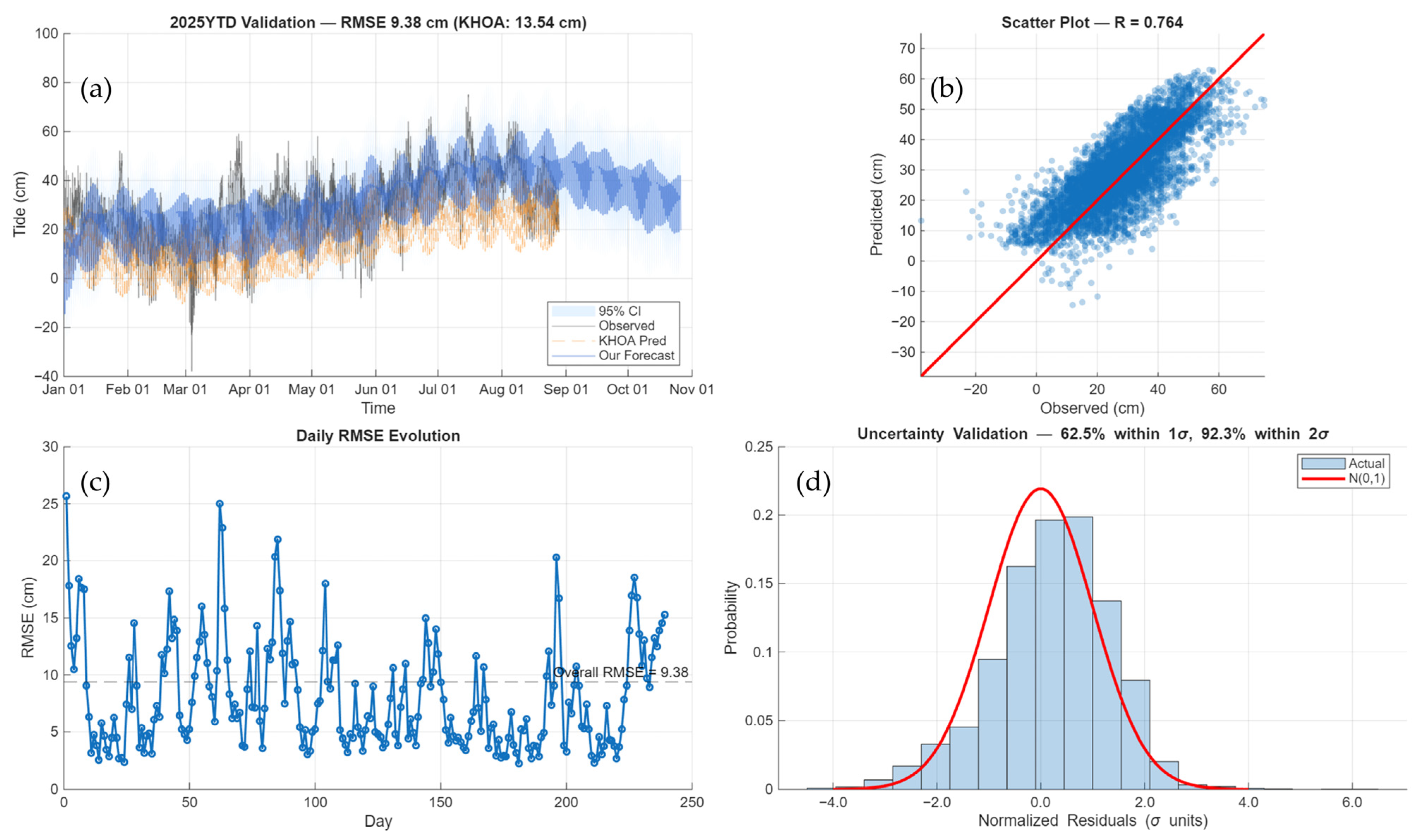
Figure A4. Mukho (South Korea) detailed performance analysis. (a) 2025YTD validation time series with KHOA prediction and hybrid forecast. (b) Parity plot with correlation coefficient. (c) Daily RMSE evolution. (d) Uncertainty validation histogram with normalized residuals.
Sustainability 17 09579 g0a4
Figure A5. Sokcho (South Korea) long-term forecast and validation. (Top): 18.6-year time series (2015–2025) showing observed tides, hybrid HA-AI forecast, and 95% uncertainty bands. Red line marks validation period start. (Bottom): Residual analysis for 2025 validation period with ±2σ uncertainty bounds.
Sustainability 17 09579 g0a5
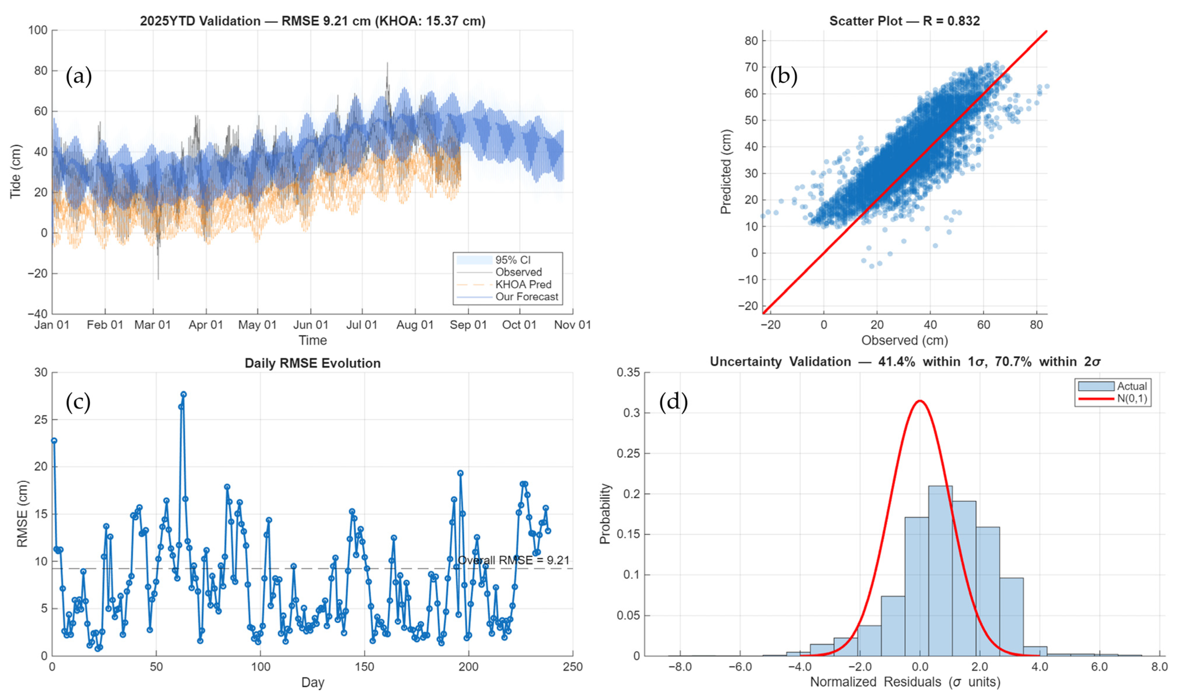
Figure A6. Sokcho (South Korea) detailed performance analysis. (a) 2025YTD validation time series with KHOA prediction and hybrid forecast. (b) Parity plot with correlation coefficient. (c) Daily RMSE evolution. (d) Uncertainty validation histogram with normalized residuals.
Sustainability 17 09579 g0a6
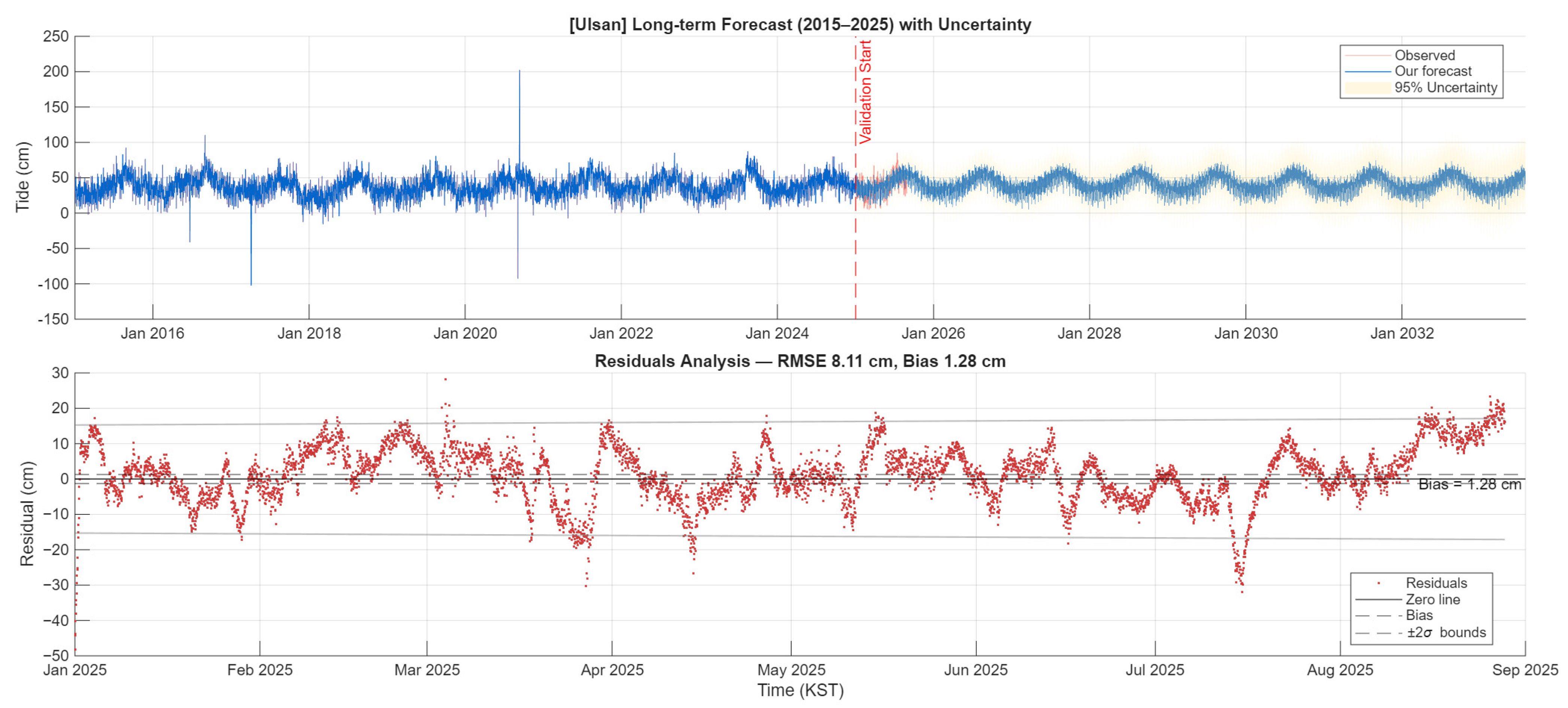
Figure A7. Ulsan (South Korea) long-term forecast and validation. (Top): 18.6-year time series (2015–2025) showing observed tides, hybrid HA-AI forecast, and 95% uncertainty bands. Red line marks validation period start. (Bottom): Residual analysis for 2025 validation period with ±2σ uncertainty bounds.
Sustainability 17 09579 g0a7
Figure A8. Ulsan (South Korea) detailed performance analysis. (a) 2025YTD validation time series with KHOA prediction and hybrid forecast. (b) Parity plot with correlation coefficient. (c) Daily RMSE evolution. (d) Uncertainty validation histogram with normalized residuals.
Sustainability 17 09579 g0a8

Appendix B

This appendix presents comprehensive three-way comparison analyses for Sokcho, Ulsan, Hupo, and Mukho stations, following the same format as Figure 7 (Busan) in the main text. Each station includes time series comparisons, residual analysis, scatter plots, and error distribution box plots.
Figure A9. Time series panel (top): Hupo presents the most challenging prediction environment due to complex nearshore bathymetry and riverine influence. Observed values (black) show increased high-frequency variability compared to other stations. HA-only predictions (orange) maintain reasonable phase alignment but with −10.1 cm bias. Hybrid predictions (blue) achieve modest but consistent improvement despite local complexity. Residual panel (middle): Higher baseline variability evident in both HA-only (RMSE = 12.89 cm) and hybrid (RMSE = 10.78 cm) residuals compared to other stations. Improvement (16.3%) is lowest among all sites, suggesting local hydrodynamic complexity approaches the limits of purely time-series-based AI correction. Enhanced performance might require incorporating additional environmental variables (wind, river discharge, stratification). Scatter panel (bottom): Moderate correlation for both methods (HA: R = 0.776; hybrid: R = 0.763) with increased scatter around 1:1 line. Data clustering reveals bimodal pattern potentially related to distinct hydrodynamic regimes (e.g., stratified vs. well-mixed conditions). Hybrid approach reduces systematic offset but inherits some irreducible uncertainty from complex local forcing.
Sustainability 17 09579 g0a9
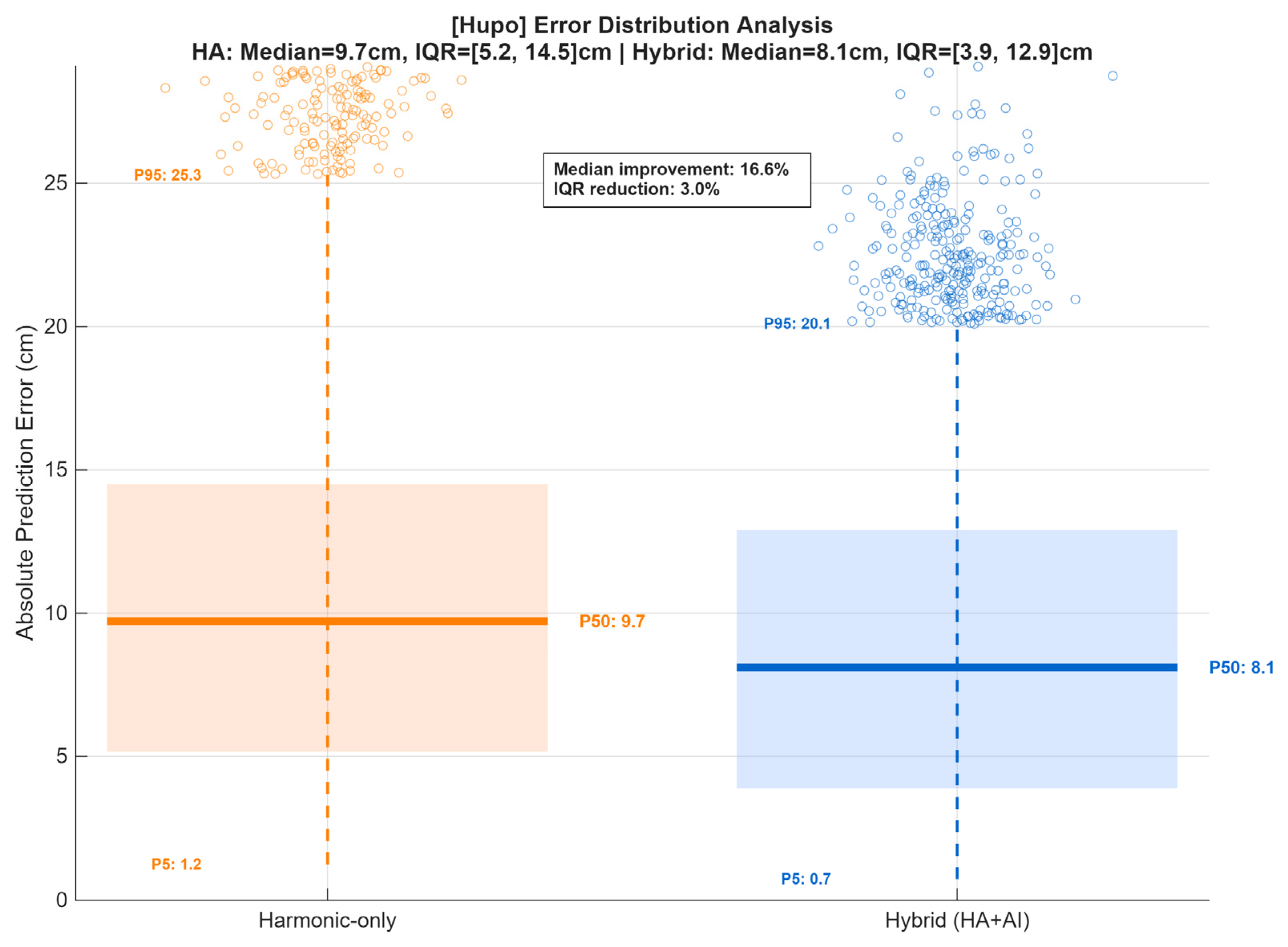
Figure A10. Error distribution analysis for Hupo station comparing harmonic-only and hybrid (HA + AI) tide predictions during the 2025 validation period. The shaded boxes indicate the interquartile range (IQR, 25–75%), thick horizontal lines mark the median (P50), and dashed lines show the 5th–95th percentile range. Outliers above the 95th percentile are plotted as open circles. The harmonic-only model shows higher median and wider IQR (median = 9.7 cm, IQR = [5.2, 14.5] cm), while the hybrid model demonstrates significantly reduced errors (median = 8.1 cm, IQR = [3.9, 12.9] cm), corresponding to a 16.6% median improvement and a 3.0% reduction in IQR.
Sustainability 17 09579 g0a10
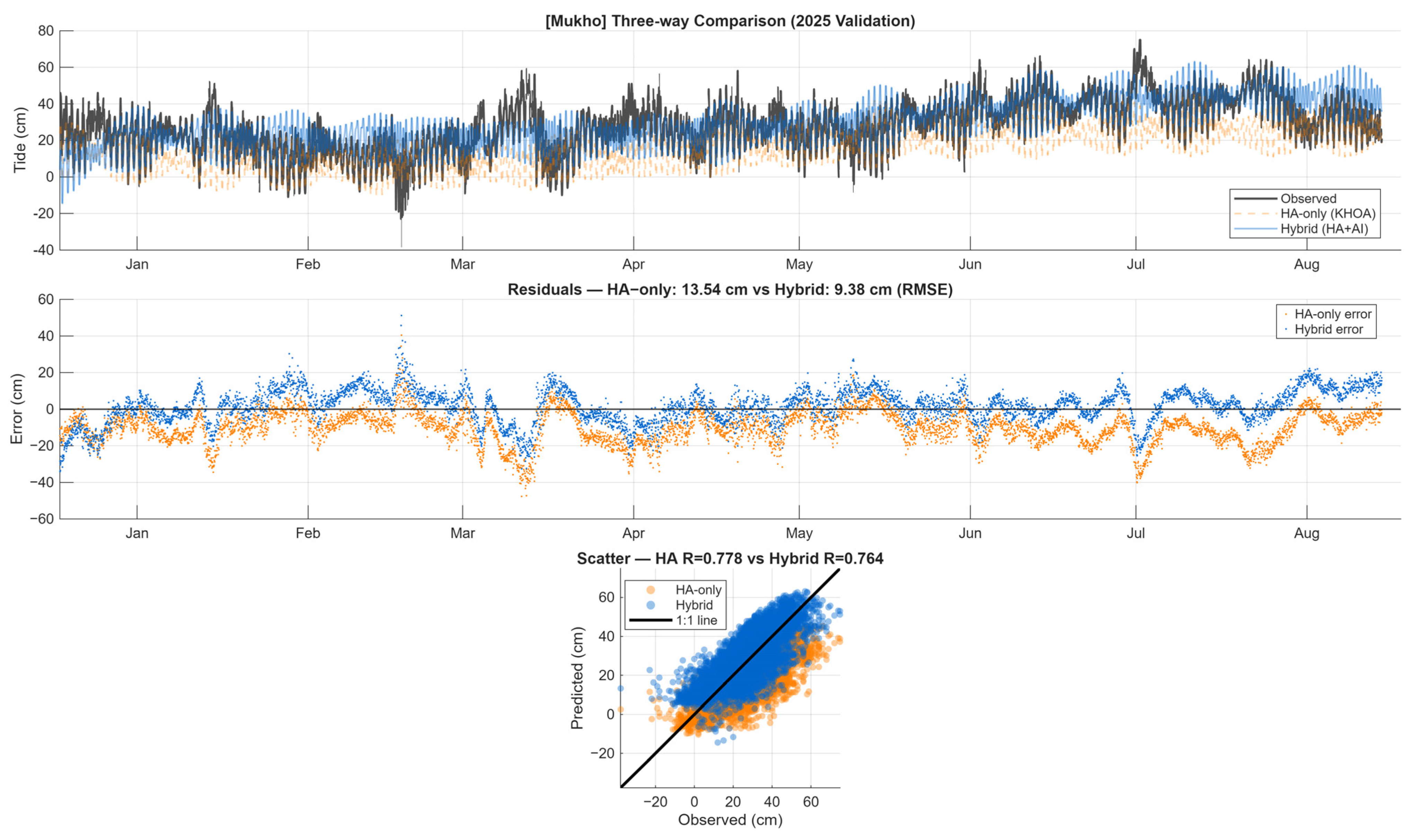
Figure A11. Time series panel (top): Mukho exhibits moderate-to-high tidal variability with pronounced spring–neap modulation. HA-only predictions (orange) show systematic −10.3 cm underprediction, particularly evident during spring tides (January–February, July–August). Hybrid predictions (blue) track observed values (black) with substantially improved accuracy across all tidal phases. Residual panel (middle): HA-only residuals (orange) demonstrate clear spring–neap periodicity with amplitude varying from −5 to −40 cm during successive tidal cycles (RMSE = 13.54 cm). Hybrid residuals (blue) show reduced systematic structure and scatter (RMSE = 9.38 cm, 30.7% improvement). Residual autocorrelation substantially reduced, indicating effective correction of deterministic biases. Scatter panel (bottom): Both methods achieve moderate correlation (HA: R = 0.778; hybrid: R = 0.764), with hybrid showing improved linearity. Orange points reveal consistent negative offset increasing with tidal magnitude; blue points center more closely on 1:1 line. Slight heteroscedasticity (increasing scatter at higher tides) suggests residual nonlinear effects requiring further investigation.
Sustainability 17 09579 g0a11
Figure A12. Error distribution analysis for Mukho station comparing harmonic-only and hybrid (HA + AI) tide predictions during the 2025 validation period. The shaded boxes indicate the interquartile range (IQR, 25–75%), thick horizontal lines mark the median (P50), and dashed lines show the 5th–95th percentile range. Outliers above the 95th percentile are plotted as open circles. The harmonic-only model shows higher median and wider IQR (median = 10.1 cm, IQR = [5.3, 15.6] cm), while the hybrid model demonstrates significantly reduced errors (median = 6.2 cm, IQR = [3.0, 10.8] cm), corresponding to a 37.9% median improvement and a 24.4% reduction in IQR.
Sustainability 17 09579 g0a12
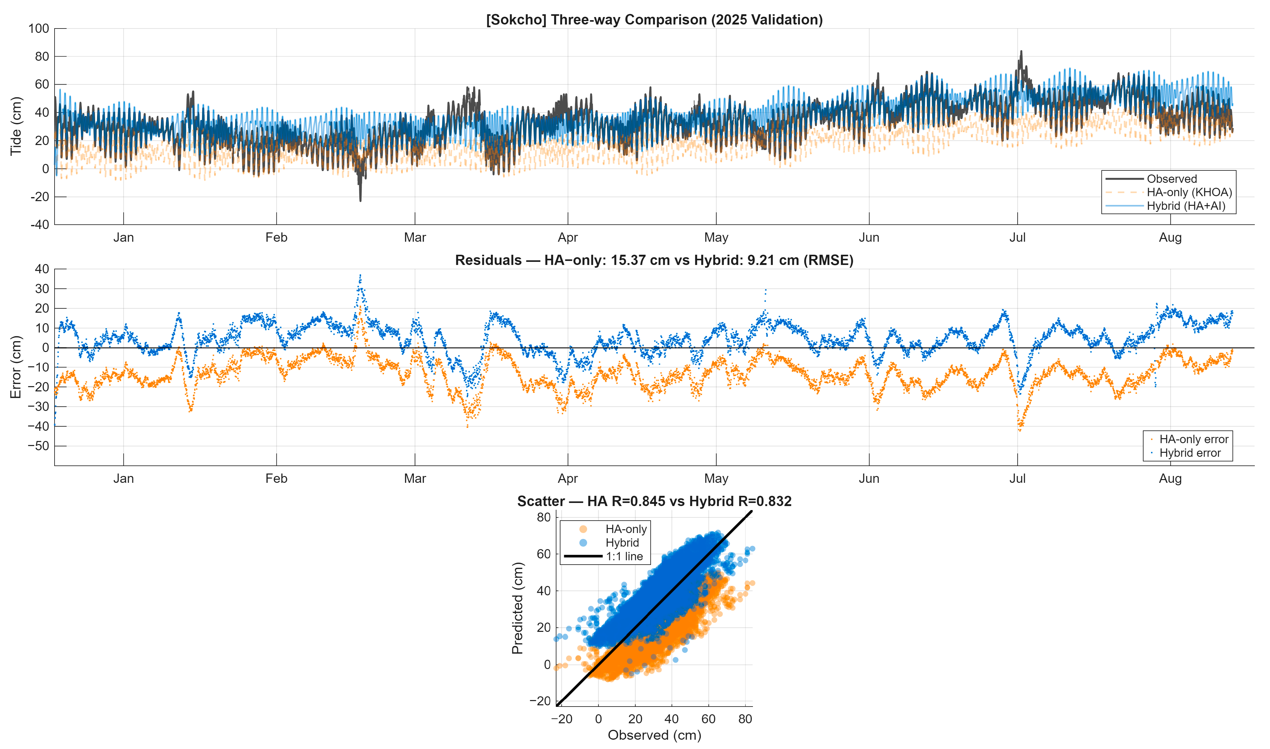
Figure A13. Time series panel (top): Nine-month continuous predictions (January–September 2025) showing observed sea level (black solid line), harmonic analysis alone from KHOA (orange dashed line), and hybrid HA-AI predictions (blue solid line). Sokcho exhibits the highest RMSE improvement (40.1%) among all stations, with hybrid predictions closely tracking observed spring–neap cycles. The persistent negative bias in HA-only predictions (approximately −13 cm) is particularly evident during summer months (July–August) when tidal ranges exceed 60 cm. Residual panel (middle): Error time series demonstrating systematic bias correction. HA-only residuals (orange points) show consistent underprediction with RMSE = 15.37 cm, while hybrid residuals (blue points) distribute more symmetrically around zero (RMSE = 9.21 cm, 40.1% improvement). Notable outlier events in early March and late July correspond to documented storm surge episodes. Scatter panel (bottom): Prediction accuracy comparison against observations. Both methods maintain moderate-to-high correlation (HA: R = 0.845; hybrid: R = 0.832), but hybrid approach shows substantially tighter clustering along the 1:1 line, particularly for mid-range tidal heights (20–50 cm). Orange points reveal systematic offset below the ideal line; blue points demonstrate improved centering.
Sustainability 17 09579 g0a13
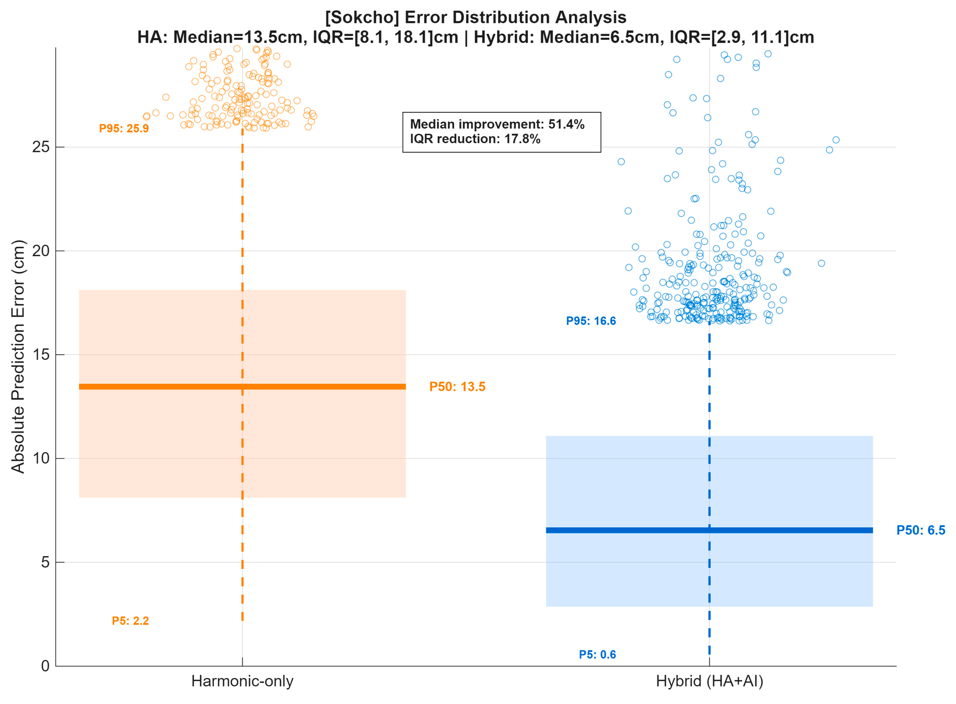
Figure A14. Error distribution analysis for Sokcho station comparing harmonic-only and hybrid (HA + AI) tide predictions during the 2025 validation period. The shaded boxes indicate the interquartile range (IQR, 25–75%), thick horizontal lines mark the median (P50), and dashed lines show the 5th–95th percentile range. Outliers above the 95th percentile are plotted as open circles. The harmonic-only model shows higher median and wider IQR (median = 13.5 cm, IQR = [8.1, 18.1] cm), while the hybrid model demonstrates significantly reduced errors (median = 6.5 cm, IQR = [2.9, 11.1] cm), corresponding to a 51.4% median improvement and a 17.8% reduction in IQR.
Sustainability 17 09579 g0a14
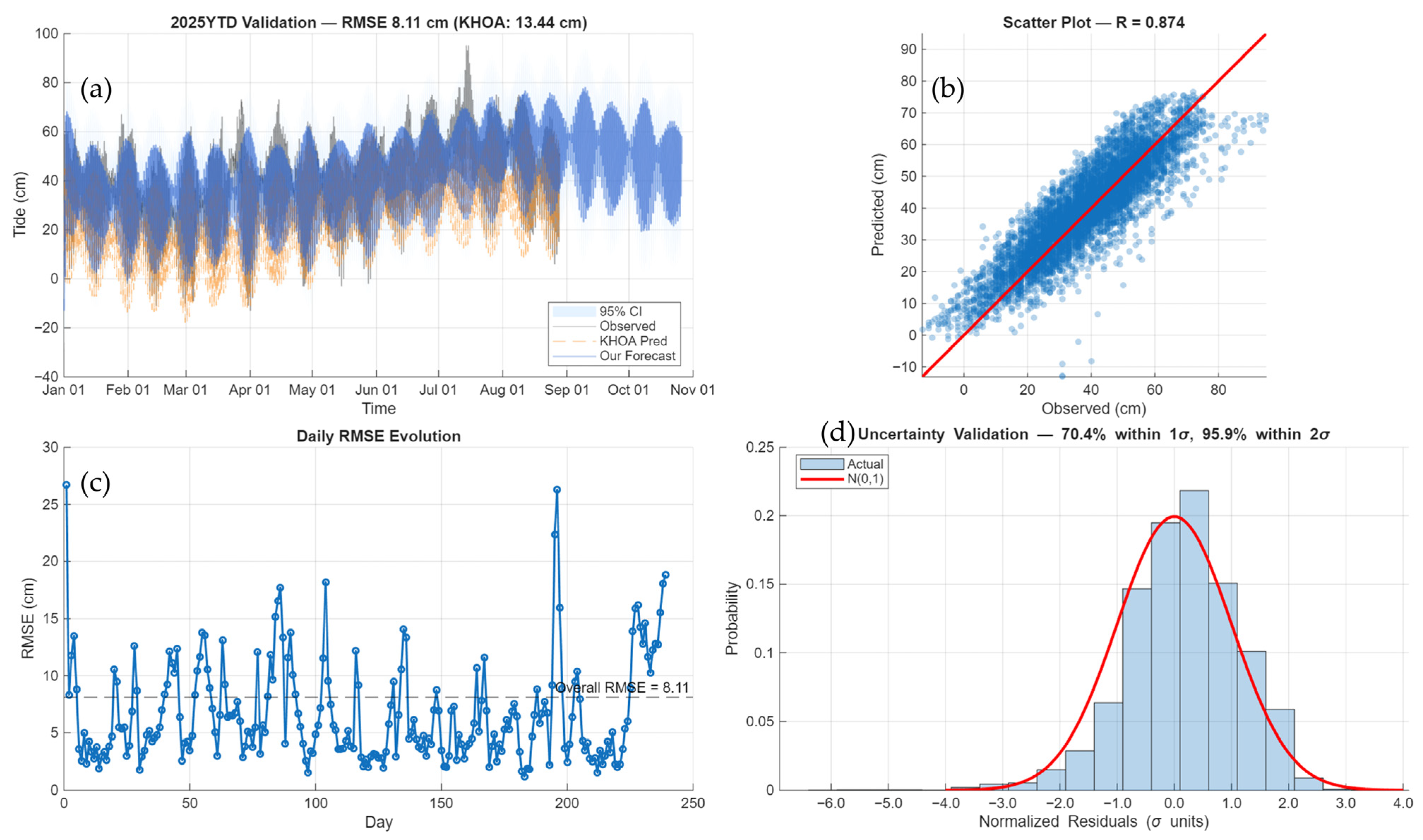
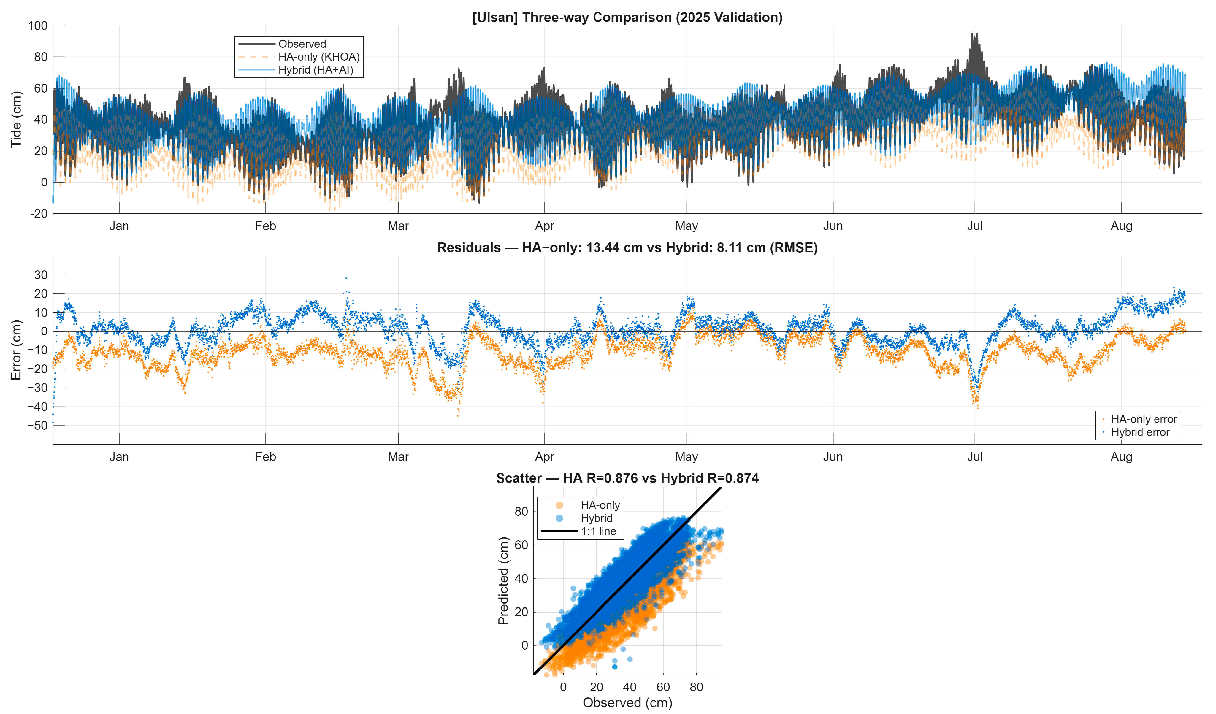
Figure A15. Time series panel (top): Ulsan predictions demonstrate excellent performance across all tidal conditions. Observed values (black) show characteristic East Sea diurnal inequality. HA-only predictions (orange) maintain phase coherence but exhibit persistent −10.7 cm bias. Hybrid predictions (blue) successfully eliminate this offset while preserving tidal phase relationships. Residual panel (middle): HA-only errors (orange) display low-frequency modulation with ~14-day periodicity, indicating incomplete shallow-water constituent representation. Hybrid residuals (blue) show reduced amplitude and less systematic structure (RMSE reduction: 13.44 → 8.11 cm, 39.7% improvement). The near-zero mean of hybrid residuals confirms effective bias correction. Scatter panel (bottom): High correlation maintained for both methods (HA: R = 0.876; hybrid: R = 0.874), with minimal correlation trade-off (ΔR = −0.002). Hybrid points cluster more tightly along 1:1 line across entire observed range (0–80 cm), demonstrating consistent accuracy improvement independent of tidal magnitude.
Sustainability 17 09579 g0a15
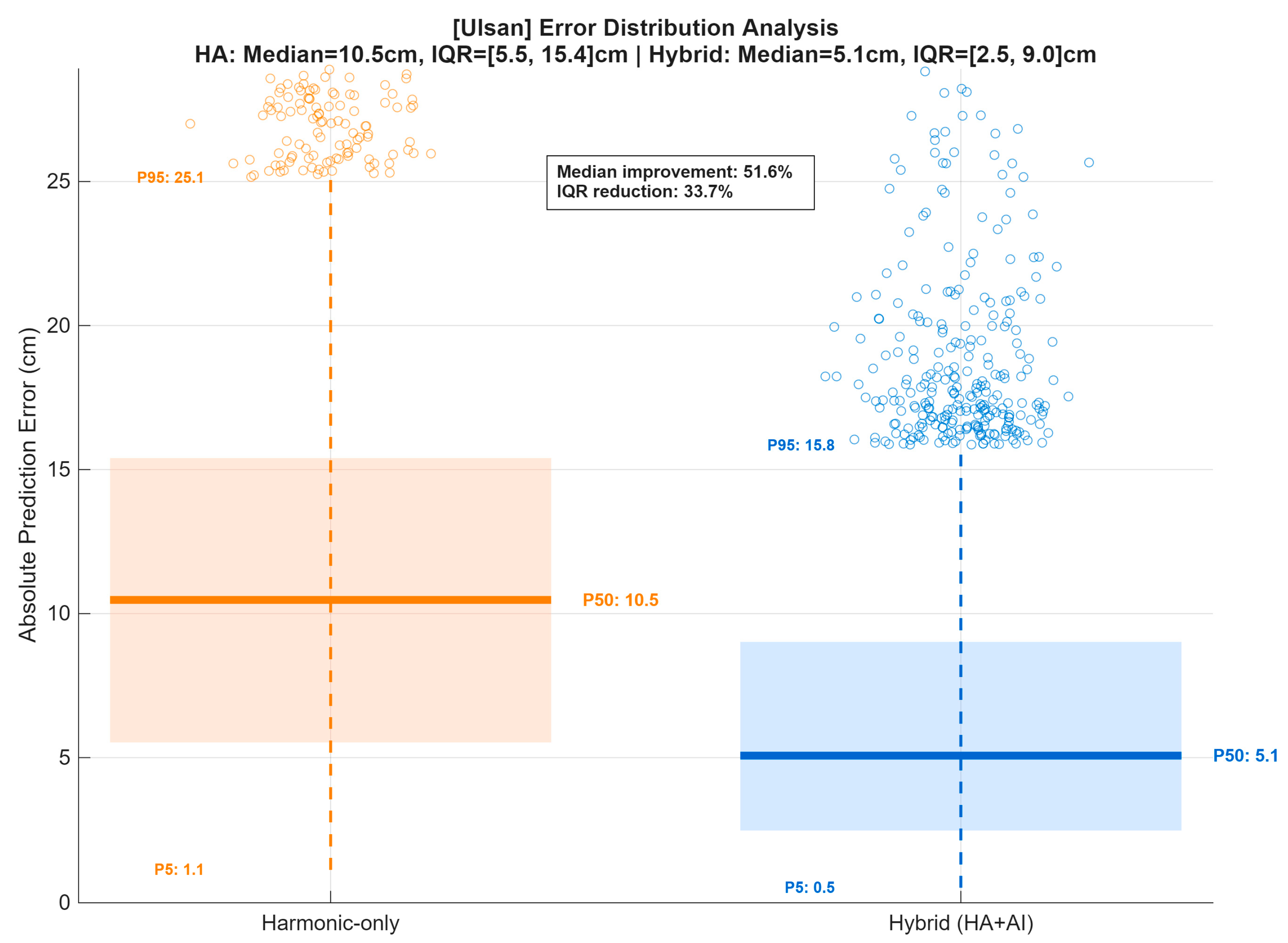
Figure A16. Error distribution analysis for Ulsan station comparing harmonic-only and hybrid (HA + AI) tide predictions during the 2025 validation period. The shaded boxes indicate the interquartile range (IQR, 25–75%), thick horizontal lines mark the median (P50), and dashed lines show the 5th–95th percentile range. Outliers above the 95th percentile are plotted as open circles. The harmonic-only model shows higher median and wider IQR (median = 10.5 cm, IQR = [5.5, 15.4] cm), while the hybrid model demonstrates significantly reduced errors (median = 5.1 cm, IQR = [2.5, 9.0] cm), corresponding to a 51.6% median improvement and a 33.7% reduction in IQR.
Sustainability 17 09579 g0a16
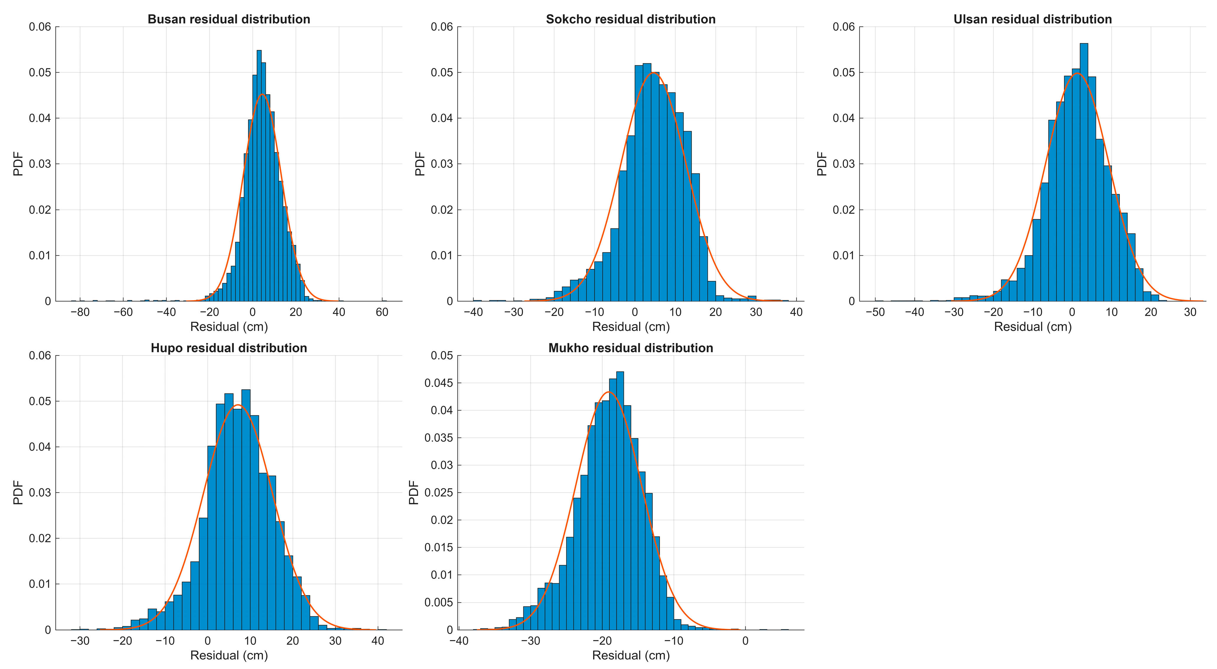
Figure A17. Probability density functions (PDFs) of hybrid model residuals for all five coastal stations during the 2025 validation period. Blue histograms represent empirical residual distributions (bin width: 2 cm); orange curves show fitted Gaussian distributions for reference. All stations demonstrate approximately normal distributions centered near zero, confirming effective bias elimination.
Sustainability 17 09579 g0a17

References

  1. Foreman, M.G.G.; Henry, R.F. The Harmonic Analysis of Tidal Model Time Series. Adv. Water Resour. 1989, 12, 109–120. [Google Scholar] [CrossRef]
  2. Foreman, M.G.G.; Cherniawsky, J.Y.; Ballantyne, V.A. Versatile Harmonic Tidal Analysis: Improvements and Applications. J. Atmos. Ocean. Technol. 2009, 26, 806–817. [Google Scholar] [CrossRef]
  3. Wan, Y. Harmonic Analysis in Tide Analysis. In Proceedings of the Second International Conference on Statistics, Applied Mathematics, and Computing Science (CSAMCS 2022), Nanjing, China, 25–27 November 2022; Jin, S., Dai, W., Eds.; SPIE: Nanjing, China, 2023; p. 134. [Google Scholar]
  4. Abubakar, A.G.; Mahmud, M.R.; Tang, K.K.W.; Hussaini, A.; Md Yusuf, N.H. A review of modelling approaches on tidal analysis and prediction. Int. Arch. Photogramm. Remote Sens. Spat. Inf. Sci. 2019, XLII-4/W16, 23–34. [Google Scholar] [CrossRef]
  5. Monahan, T.; Tang, T.; Roberts, S.; Adcock, T.A.A. Tidal Corrections From and for SWOT Using a Spatially Coherent Variational Bayesian Harmonic Analysis. J. Geophys. Res. Ocean. 2025, 130, e2024JC021533. [Google Scholar] [CrossRef]
  6. Ghamati, E.; Kariman, H.; Hoseinzadeh, S. Experimental and Computational Fluid Dynamic Study of Water Flow and Submerged Depth Effects on a Tidal Turbine Performance. Water 2023, 15, 2312. [Google Scholar] [CrossRef]
  7. Liang, S.X.; Li, M.C.; Sun, Z.C. Prediction Models for Tidal Level Including Strong Meteorologic Effects Using a Neural Network. Ocean Eng. 2008, 35, 666–675. [Google Scholar] [CrossRef]
  8. Liu, J.; Shi, G.; Zhu, K. High-Precision Combined Tidal Forecasting Model. Algorithms 2019, 12, 65. [Google Scholar] [CrossRef]
  9. Zhang, Z.; Zhang, L.; Yue, S.; Wu, J.; Guo, F. Correction of Nonstationary Tidal Prediction Using Deep-Learning Neural Network Models in Tidal Estuaries and Rivers. J. Hydrol. 2023, 622, 129686. [Google Scholar] [CrossRef]
  10. Zhu, Z.; Yan, X.; Wang, Z.; Liu, S. Spatiotemporal Prediction of Tidal Fields in a Semi-Enclosed Marine Bay Using Deep Learning. Water 2025, 17, 386. [Google Scholar] [CrossRef]
  11. Huang, X.; Tang, J.; Shen, Y.; Zhang, C. Predicting and Analyzing the Three-Dimensional Spatiotemporal Evolution Process of Tidal Currents by Using a Brand New Machine Learning Algorithm. Phys. Fluids 2025, 37, 016609. [Google Scholar] [CrossRef]
  12. Ban, W.; Shen, L.; Lu, F.; Liu, X.; Pan, Y. Research on Long-Term Tidal-Height-Prediction-Based Decomposition Algorithms and Machine Learning Models. Remote Sens. 2023, 15, 3045. [Google Scholar] [CrossRef]
  13. Qian, P.; Feng, B.; Liu, X.; Zhang, D.; Yang, J.; Ying, Y.; Liu, C.; Si, Y. Tidal Current Prediction Based on a Hybrid Machine Learning Method. Ocean Eng. 2022, 260, 111985. [Google Scholar] [CrossRef]
  14. Fei, K.; Du, H.; Gao, L. Accurate Water Level Predictions in a Tidal Reach: Integration of Physics-Based and Machine Learning Approaches. J. Hydrol. 2023, 622, 129705. [Google Scholar] [CrossRef]
  15. Wu, J.; Guo, J.; Wu, J. Physics-Informed Hybrid Model for Scour Evolution Prediction around Pile Foundations under Tidal Currents. Phys. Fluids 2025, 37, 047130. [Google Scholar] [CrossRef]
  16. Pugh, D.T.; Woodworth, P.L. Sea-Level Science: Understanding Tides, Surges, Tsunamis and Mean Sea-Level Changes; Cambridge University Press: Cambridge, UK, 2014; ISBN 978-1-107-02819-7. [Google Scholar] [CrossRef]
  17. Peng, D.; Hill, E.M.; Meltzner, A.J.; Switzer, A.D. Tide Gauge Records Show That the 18.61-Year Nodal Tidal Cycle Can Change High Water Levels by up to 30 cm. J. Geophys. Res. Ocean. 2019, 124, 736–749. [Google Scholar] [CrossRef]
  18. Saintilan, N.; Lymburner, L.; Wen, L.; Haigh, I.D.; Ai, E.; Kelleway, J.J.; Rogers, K.; Pham, T.D.; Lucas, R. The Lunar Nodal Cycle Controls Mangrove Canopy Cover on the Australian Continent. Sci. Adv. 2022, 8, eabo6602. [Google Scholar] [CrossRef] [PubMed]
  19. Pan, H.; Wei, Y.; Xu, T.; Wei, Z. A Time-Varying Tidal Form Factor Considering the 18.61-Year Nodal Cycle. Estuar. Coast. Shelf Sci. 2024, 305, 108868. [Google Scholar] [CrossRef]
  20. Coelho, A.D.L.; Gireli, T.Z.; Venancio, K.K.; Garcia, P.D. Exploring Tidal Constituent Trends: Unveiling the Impact of the 18.6-Year Lunar Nodal Cycle through Harmonic Analysis and Long-Term Tide Gauge Records. J. Integr. Coast. Zone Manag. 2024, 24, 41–53. [Google Scholar] [CrossRef]
  21. Pappas, K.; Mackie, L.; Zilakos, I.; Van Der Weijde, A.H.; Angeloudis, A. Sensitivity of Tidal Range Assessments to Harmonic Constituents and Analysis Timeframe. Renew. Energy 2023, 205, 125–141. [Google Scholar] [CrossRef]
  22. Haigh, I.D.; Eliot, M.; Pattiaratchi, C. Global Influences of the 18.61 Year Nodal Cycle and 8.85 Year Cycle of Lunar Perigee on High Tidal Levels. J. Geophys. Res. 2011, 116, C06025. [Google Scholar] [CrossRef]
  23. Monahan, T.; Tang, T.; Adcock, T.A.A. A Hybrid Model for Online Short-Term Tidal Energy Forecasting. Appl. Ocean Res. 2023, 137, 103596. [Google Scholar] [CrossRef]
  24. Yang, C.-H.; Wu, C.-H.; Hsieh, C.-M. Long Short-Term Memory Recurrent Neural Network for Tidal Level Forecasting. IEEE Access 2020, 8, 159389–159401. [Google Scholar] [CrossRef]
  25. Riazi, A. Accurate Tide Level Estimation: A Deep Learning Approach. Ocean Eng. 2020, 198, 107013. [Google Scholar] [CrossRef]
  26. Willard, J.; Jia, X.; Xu, S.; Steinbach, M.; Kumar, V. Integrating Scientific Knowledge with Machine Learning for Engineering and Environmental Systems. ACM Comput. Surv. 2023, 55, 1–37. [Google Scholar] [CrossRef]
  27. Delligatti, A.; Kong, L. Integrating Physics and Machine Learning: A Synergistic Approach to Artificial Intelligence Education. In Proceedings of the 2024 6th International Workshop on Artificial Intelligence and Education (WAIE), Tokyo, Japan, 28–30 September 2024; IEEE: Tokyo, Japan, 2024; pp. 342–346. [Google Scholar]
  28. Dominguez, A.; De La Garza, J.; Quezada-Espinoza, M.; Zavala, G. Integration of Physics and Mathematics in STEM Education: Use of Modeling. Educ. Sci. 2023, 14, 20. [Google Scholar] [CrossRef]
Figure 1. Study area and site locations. (a) Regional setting in Northeast Asia showing the Korean Peninsula and the East Sea sector investigated. (b) Detailed map of Korea’s east coast indicating the five study sites (Sokcho, Mukho, Hupo, Ulsan, and Busan, marked with red circles).
Sustainability 17 09579 g001
Figure 2. Hourly tidal observations from 2015–2024 were preprocessed and decomposed using harmonic analysis with nodal adjustment. Residual signals were extracted and modeled through AI-based techniques, enabling a hybrid forecast that integrates deterministic and adaptive components. The reconstructed 18.6-year equivalent record was then analyzed for long-term sea-level trends using statistical methods, with the final outputs interpreted in the context of coastal resilience and sustainability.
Sustainability 17 09579 g002
Figure 3. Variance partition analysis across five stations. (a) Constituent-wise variance contributions based on nodally adjusted harmonic analysis (HA), showing spatial differences in tidal dynamics across stations. (b) Cumulative variance explained (%) by top-k leading constituents, highlighting rapid saturation at open-coast sites (e.g., Busan) compared to semi-enclosed sites. (c) Residual variance fraction (%) not captured by HA, indicating site-specific non-tidal influences requiring AI-based modeling.
Sustainability 17 09579 g003
Figure 4. Busan long-term forecast and validation. (Top): 18.6-year time series (2015–2025) showing observed tides (black), the hybrid HA–AI forecast (blue), and 95% uncertainty bands (light-blue shading). The red dashed line marks the start of the 2025 validation period. For readability, the time-series curves are down-sampled at plot time (constant stride); all statistics are computed from the full-resolution data. (Bottom): Residual analysis for the 2025 validation period with ±2σ uncertainty bounds (gray lines). Performance: RMSE = 9.87 cm, Bias = 4.43 cm.
Sustainability 17 09579 g004
Figure 5. Global performance of the hybrid HA-AI forecast across five stations during 2025 validation period. (a) 2025YTD validation time series comparing observed (black), KHOA prediction (orange), and hybrid forecast (blue) with 95% uncertainty band (light blue shading). (b) Parity plot showing strong agreement with 1:1 line (R = 0.960). (c) Daily RMSE evolution demonstrating consistent performance throughout validation period. (d) Uncertainty validation histogram with normalized residuals; 24.2% within 1σ and 46.2% within 2σ bounds confirm well-calibrated uncertainty estimates.
Sustainability 17 09579 g005
Figure 6. Three-way comparison of tidal predictions at Busan station (2025 validation period). Top: nine-month time series showing observed (black), harmonic analysis alone (orange), and hybrid HA-AI (blue) predictions. Middle: residual time series demonstrating systematic bias elimination (HA-only RMSE: 15.11 cm; hybrid RMSE: 9.87 cm). Bottom: scatter plots comparing prediction accuracy; hybrid approach maintains high correlation (R = 0.960) while reducing RMSE by 34.7%. Orange points show persistent underprediction bias in HA-only method; blue points demonstrate improved accuracy along 1:1 line.
Sustainability 17 09579 g006
Figure 7. Error distribution analysis for Busan station comparing harmonic-only and hybrid (HA + AI) tide predictions during the 2025 validation period. The shaded boxes indicate the interquartile range (IQR, 25–75%), thick horizontal lines mark the median (P50), and dashed lines show the 5th–95th percentile range. Outliers above the 95th percentile are plotted as open circles. The harmonic-only model shows higher median and wider IQR (median = 12.5 cm, IQR = [7.8, 17.5] cm), while the hybrid model demonstrates significantly reduced errors (median = 6.0 cm, IQR = [2.8, 10.8] cm), corresponding to a 52.3% median improvement and a 17.8% reduction in IQR.
Sustainability 17 09579 g007
Figure 8. Monthly distributions of RMSE, MAE, and correlation coefficient (R) for the hybrid HA–AI model across five tide gauge stations during the validation period.
Sustainability 17 09579 g008
Figure 9. The left panel presents a station–metric heat map of error indicators, including the root mean square error (RMSE), mean absolute error (MAE), and absolute bias (|Bias|) for the five validation stations (Busan, Sokcho, Ulsan, Hupo, and Mukho). The right panel shows the station-wise correlation coefficients (R) in a dotted line plot, as suggested by the reviewer, illustrating the spatial variation in predictive accuracy. The high correlation values (R > 0.75) across all sites indicate that the hybrid LSTM model maintains robust consistency among diverse coastal environments.
Sustainability 17 09579 g009
Table 1. Tidal constituent amplitudes and phases across five tide-gauge stations along the eastern coast of Korea. Harmonic constants for the four dominant constituents (M2, S2, K1, O1) derived from T_Tide (Version 1.4) analysis of hourly sea-level observations (2015–2024). Amplitudes are in centimeters above mean sea level; phases are Greenwich phase lags in degrees with nodal corrections applied. These constants provide the baseline astronomical forcing for hybrid HA–AI tidal modeling.
StationM2 S2 K1 O1
Amp (cm)Phase (°)Amp (cm)Phase (°)Amp (cm)Phase (°)Amp (cm)Phase (°)
Busan35.224512.92784.12351.6252
Sokcho0.78512751.63252.5340
Ulsan10.22603.52802.12701.8315
Hupo1.8850.7903.73252340
Mukho3.2850.4952.83302.5350
Notes: Amplitudes are given in centimeters above mean sea level. Phases are Greenwich phase lags in degrees, referenced to the record midpoint with nodal corrections applied. Values derived from T_Tide (Version 1.4) harmonic analysis of hourly observations (2015–2024) using 68-constituent decomposition. M2 = principal lunar semidiurnal; S2 = solar semidiurnal; K1 = lunar diurnal; O1 = principal diurnal.
Table 2. Comparative Performance: Harmonic Analysis vs. Hybrid Framework (2025 Validation).
StationHA-Only RMSE (cm)Hybrid RMSE (cm)Improvement (%)HA-only RHybrid R
Busan15.119.8734.70.9670.960
Sokcho15.379.2140.10.8450.832
Ulsan13.448.1139.70.8760.874
Hupo12.8910.7816.30.7760.763
Mukho13.549.3830.70.7780.764
Average14.079.4732.30.8480.839
Table 3. Performance metrics for hybrid HA-AI tidal forecasts across five stations during 2025 validation period.
StationRMSE (cm)MAE (cm)Bias (cm)RRMSE_KHOA (cm)Improvement (%)
Busan9.877.524.430.96015.1134.7
Sokcho9.217.424.590.83215.3740.1
Ulsan8.116.311.280.87413.4439.7
Hupo10.788.897.110.76312.8916.3
Mukho9.387.461.800.76413.5430.7
Average9.477.523.840.83914.0732.3
Disclaimer/Publisher’s Note: The statements, opinions and data contained in all publications are solely those of the individual author(s) and contributor(s) and not of MDPI and/or the editor(s). MDPI and/or the editor(s) disclaim responsibility for any injury to people or property resulting from any ideas, methods, instructions or products referred to in the content.