Abstract
(1) Background: Climate change has intensified extreme heat and localized rainfall, exposing South Korea’s protected trees to new risks. Despite their ecological and cultural value, prior research has been largely local or qualitative, leaving little basis for nationwide prioritization. (2) Methods: We developed a composite risk index that integrates heat and rainfall exposure with species sensitivities, covering nearly the entire national inventory (≈10,000 individuals). Risks were calculated at the tree level, aggregated to district, provincial, and national scales, and tested for robustness across weighting and normalization choices. Spatial clustering was assessed with Moran’s I and LISA. (3) Results: High-risk clusters were consistently identified in southern and southwestern regions. Mean and tail indicators showed that average-based approaches obscure extreme vulnerabilities, while LISA confirmed significant High–High clusters. Rankings proved robust across scenarios, indicating that results reflect structural signals rather than parameter settings. Priority areas defined by the presence of extreme-risk individuals emerged as stable candidates for intervention. (4) Conclusions: The study establishes a transparent, operational rule for prioritization and offers tailored strategies—such as drainage infrastructure, shading, and root-zone management—while informing medium-term planning. It provides the first nationwide, empirically grounded framework for conserving protected trees under climate transition.
1. Introduction
1.1. Research Background
Trees provide foundational ecological and socio-cultural functions, yet conservation regimes remain fragmented, especially for trees outside forests and monument trees. Recent syntheses estimate that about 30% of the world’s tree species are threatened with extinction and call for policy toolkits that go beyond forest-centric approaches [1].
The increasing frequency and intensity of extreme heat and localized heavy rainfall due to climate change are generating new types of risks across ecosystems and cultural landscapes. Protected trees (Bohosu) serve as cultural–ecological assets that embody the historical and place-specific identity of their respective regions. Their vulnerability is determined not only by intrinsic physiological characteristics—such as species-specific tolerance to heat and rainfall, root-zone soil conditions, and canopy structure—but also by the degree of climate exposure (e.g., days of extreme heat, records of heavy precipitation) and the effectiveness of management systems (inspection cycles, irrigation and drainage practices, pest and disease control).
Despite this complexity, administrative practice in South Korea has generally relied on averages at the administrative-unit level or post-disaster statistics to assess regional vulnerability. Existing domestic and international studies have similarly tended to report localized conditions of protected trees [2,3,4,5,6,7] or to focus on how to improve the management of individual specimens [8]. In some cases, research has proposed detailed evaluation criteria for protected tree management [9] or examined legal protections [10]. Yet even these studies remain largely qualitative and seldom address the implications of climate transition. Consequently, they provide little guidance for policy-level decision-making on which protected trees or regions should be prioritized in the era of climate crisis.
This limitation has also been noted internationally. Some Authors, like Wyse, Beggs, Burns, and Stanley [11], identified the common shortcoming of approaches that rely exclusively on the protection of individual trees, highlighting the need for strategies at national and local government scales. Similarly, Caiche, Peres, and Schenk [12] explored tree-protection strategies from a historical perspective at the urban level, extending the discussion beyond individual care to a broader spatial scale. Nevertheless, such studies still fall short of quantitatively assessing relative risks at the individual level, spatially organizing those risks, and providing a systematic framework for strategic prioritization in policy and management. While prior global overviews have articulated the importance, tools, and challenges of protecting trees—including TOFs and monument trees—such works remain largely conceptual [1].
To address this gap, the present study integrates the locational and species information of approximately 10,000 protected trees across South Korea with district-level indicators of heat and rainfall. By constructing a composite risk index at the individual-tree level and aggregating it across multiple scales (national, provincial, district, and species), the study establishes a framework for systematic interpretation and prioritization of conservation efforts.
1.2. Research Objectives and Questions
The primary objective of this study is to calculate a composite risk index for protected trees across South Korea by integrating climate exposure (heat and rainfall) with species-specific sensitivities at the individual-tree level, and to systematically describe its spatial distribution. By doing so, the study aims to provide administrative and management authorities with an empirical basis for rationally determining the order of inspection and intervention under limited budgets and personnel. To this end, the following research questions are posed:
RQ1: What species of protected trees exist across South Korea, and what distinctive climate vulnerabilities characterize each region? (Section 3.1)
RQ2: How can a composite risk index—one that incorporates both species-specific sensitivities to heat and rainfall and region-specific climate vulnerabilities—be calculated, and how does it vary at the national, provincial, and district levels? (Section 3.2)
RQ3: Which counties exhibit particularly high levels of composite risk, how can these be categorized by type (heat-driven, rainfall-driven, species-sensitivity-driven, or combined), and how do risks differ across species? (Section 3.3)
RQ4: How can the spatial distribution and clustering patterns of risk be effectively visualized? (Section 3.5)
RQ5: To what extent are regional risk levels and their rankings robust when weighting schemes and normalization methods are altered? (Section 3.6)
RQ6: Based on the available data, which areas can already be identified as priority management districts, and what specific conservation strategies or policies can be most readily applied to these regions? (Section 3.4 and Section 4).
1.3. Academic and Practical Contributions
This study makes contributions on both academic and practical fronts. Academically, it advances research on the conservation of protected trees by moving beyond descriptive or case-specific analyses toward a comprehensive, quantitative, and spatially organized assessment framework. By developing a composite risk index at the individual-tree level and examining its robustness across weighting schemes, normalization methods, and spatial thresholds, the study demonstrates a methodology that can be replicated and extended in future climate-vulnerability assessments of cultural and ecological heritage assets.
Practically, the study provides a transparent and operational framework for prioritizing the management of protected trees at multiple administrative levels. The proposed rule—defining priority districts by the actual presence of extreme-risk individuals—offers decision-makers an immediately applicable criterion under conditions of limited resources. Furthermore, the integration of average and tail indicators, risk-type classification, and spatial clustering enables the design of differentiated management packages, ranging from short-term interventions to medium-term strategic planning. In doing so, the study bridges the gap between academic analysis and actionable conservation policy.
1.4. Structure of the Paper
The remainder of this paper is organized as follows. Section 1 introduces the dataset, including the scope, sources, and procedures for spatial validation. Section 2 outlines the methodology, covering normalization, species sensitivity labeling, the construction of the composite risk index, spatial statistical analysis, and robustness checks. Section 3 presents the results across multiple scales, including descriptive statistics, interregional comparisons, scenario analyses, and species-level differences. Section 4 discusses these findings in light of the research questions, emphasizing both theoretical and policy implications. Finally, Section 5 concludes by summarizing the key contributions, acknowledging limitations, and identifying directions for future research.
2. Materials and Methods
2.1. Materials
2.1.1. Scope and Sources of Data
This study integrates three strands of data. First, the dataset on individual protected trees includes information on location (latitude and longitude), administrative units (province and district), species, and selected characteristics such as height, girth, and crown width. This dataset provides the basic unit of analysis—the individual tree—while also supplying a spatial key (district-level identifier) to be linked with climate indicators. Protected-tree coordinates and attributes were compiled from the Ministry of the Interior and Safety’s portal [13]. We downloaded and merged 17 provincial Excel files that list protected trees by province.
Second, climate-related indicators of heat and rainfall are employed at the district level. These data include indices of exposure, sensitivity, and vulnerability (see Table 1 and Table 2). Since all climate indicators are defined at the district scale, each protected tree is assigned the corresponding values by joining through the district key. We used national climate vulnerability indicators disseminated by Statistics Korea [14]. In our analysis, these indicators were used at the administrative district levels. No additional spatial interpolation was performed by the authors; therefore, uncertainty stems from the source methodology (indicator construction) rather than from author-side resampling.

Table 1.
Examples of heat-related indicators for selected counties. Out of 251 counties in total, ten were randomly selected. Indicators range from 1 to 4, with lower values representing higher vulnerability.

Table 2.
Examples of rainfall-related indicators for selected counties. As with the heat indicators, there are 251 counties in total, and the same ten counties selected in Table 1 are listed here for consistency. Indicators again range from 1 to 4, with lower values indicating greater vulnerability.
Third, species-specific physiological sensitivities to heat and excessive moisture (rainfall/flooding) are quantified on a three-point scale: high (0.9), medium (0.6), and low (0.3) (see Table 3). These sensitivity scores are primarily derived from authoritative and widely used references—Silvics of North America [15,16], PFAF [17], NIBR [18], and an online plant encyclopedia [19]. Where necessary, we also consulted USDA PLANTS [20] and the CABI Compendium [21] for cross-verification. For species lacking direct sensitivity information in our sources, we used a nearest analogue approach: we referenced taxonomically and ecologically similar species (e.g., same genus or closely related species with comparable drought/heat responses) and documented this as an uncertainty source. However, it should be noted that no established reference quantitatively measures the physiological sensitivity of multiple species. Most available data are qualitative and highly limited in number. Consequently, the external validity of the sensitivity chart remains open to debate. This dataset should therefore be regarded as provisional, requiring further refinement and continuous updating through future research.

Table 3.
Examples of species-specific sensitivities to heat and rainfall (waterlogging). Species sensitivities are expressed on a three-point scale.
While national climate trend series are available, standardized time-series data on protected-tree health—necessary to verify the rationality of the model’s risk index—are unfortunately not yet available at the national level in Korea. Current records remain insufficient, sporadic, and localized. Accordingly, this study is inevitably cross-sectional, and we treat the index as a cross-sectional prioritization tool, deferring longitudinal validation to future iterations once systematic health data become available. In Section 4, we propose policy recommendations for establishing a national tree-health monitoring system to enable long-term observation of protected-tree health, mortality, and deterioration patterns.
2.1.2. Consistency of Spatial Keys, Coordinate Validation, and Treatment of Outliers
The district-level identifiers in the protected tree dataset were standardized to ensure a one-to-one correspondence with the naming conventions used in the heat and rainfall indicators. Specifically, parentheses, spaces, and variant notations (e.g., omission or duplication of “eup/myeon/dong”) as well as remnants of outdated administrative names were normalized. For cases where ambiguity remained (e.g., homonymous place names), the provincial name was added as an auxiliary key to prevent confusion.
Tree coordinates were based on WGS84 (latitude and longitude). Quality checks were performed by verifying the physical limits of latitude and longitude values and by identifying duplicate coordinates (exact matches and cases with identical registration numbers). This allowed obvious errors to be detected and corrected.
In some instances, the original dataset recorded multiple trees of different species under a single management number. These entries were variously separated by symbols such as plus signs, commas, blank spaces, or slashes. When proportional information was provided, the most frequently represented species was adopted. Where no proportional information was available, classification was guided by the family-level taxonomy, with the species most consistent with the reported family being selected. If identification remained uncertain even after these steps, the tree was conservatively assigned to the species most sensitive to heat and rainfall, in line with the precautionary principle of protected tree management.
2.2. Method
2.2.1. Normalization of Indicators (Scale Adjustment and Common Metrics)
The indices of heat and rainfall vulnerability and species sensitivity differ in both units and ranges. To facilitate weighting, combination, and comparison, it is necessary to adjust these indicators to a common scale. For the sake of comparability and interpretive consistency, this study employs linear normalization to the [0, 1] range as the default procedure. Specifically, each indicator x is transformed as follows:
Under this transformation, 0 represents relatively low vulnerability (or sensitivity), while 1 represents high vulnerability (or sensitivity). In addition to visualizing the distribution of the raw and normalized data through histograms and overlaid empirical cumulative distribution functions (ECDFs), this study also reports tail mass and quantile tables. For robustness checks, z-standardization (Z = (X − μ)/σ) is additionally employed when necessary. Unless otherwise specified, all indices reported in this study are based on [0, 1] normalization, with z-standardized results referenced only in the robustness analysis section.
2.2.2. Construction of Species Sensitivity
Species sensitivity reflects the physiological limits of individual trees (e.g., thresholds for heat tolerance, vulnerability to excessive moisture), enabling the capture of differential responses among species even under the same local conditions. While traits such as height, girth, and crown width of protected trees can serve as proxies for health status, this study does not focus on tree health per se, and thus these variables are not used as explanatory factors. Species sensitivity is instead assessed at the individual–species level.
The original heat and rainfall (waterlogging) sensitivity tables (continuous values) are first transformed into continuous scores in the [0, 1] range using the normalization method described in Section 3.1 (0 = low, 1 = high). The two dimensions are then averaged with equal weights to yield the integrated sensitivity of individual i:
For policy communication, these continuous scores are additionally summarized into categorical labels (“low,” “moderate,” “high”). However, as noted earlier, most species sensitivities are qualitatively described in the literature, and the available data are too limited to justify scales more granular than a three-level categorization. Therefore, while categorical labels are provided for interpretive clarity, all calculations and aggregations in this study rely on the continuous [0, 1] scores.
2.2.3. Definition of the Composite Risk Index
This study calculates a composite risk index (Riski) for each protected tree by combining the regional indicators of heat and rainfall vulnerability with the species-specific sensitivity of the tree, scaled to the [0, 1] range. Based on this index, priority management districts are identified. The analytical focus is not on the absolute magnitude of values but on their relative rankings and spatial patterns.
The index is constructed from three normalized components: heat vulnerability (Hi), rainfall vulnerability (Ri), and species sensitivity (Si). It takes the form of a weighted sum:
Riski = wH Hi + wR Ri + wS Si, wH + wR + wS =1, w ≥ 0
Weighting schemes are varied under three scenarios (A, B, C) for comparison:
Scenario A: Heat (wH = 0.45), rainfall (wR = 0.30), species sensitivity (wS = 0.25).
Scenario B (baseline): Heat (0.35), rainfall (0.40), species sensitivity (0.25).
Scenario C: Heat (0.50), rainfall (0.25), species sensitivity (0.25).
The rationale for selecting Scenario B is as follows: in recent years, summer rainfall exposure and vulnerability signals in South Korea have shown pronounced spatial gradients, and when coupled with the sensitivities of certain protected tree species, they create a strong need for immediate management action before the summer season. Accordingly, assigning weights in the order of “rainfall ≥ heat > species sensitivity” as the baseline scenario is operationally the most natural choice. Nevertheless, as shown below, even when compared with Scenarios A and C, which assign relatively higher weights to heat, the rank correlations remain high, ensuring that conclusions remain robust when Scenario B is used as the reference.
Scenarios A and C both emphasize heat vulnerability, though A is slightly more balanced, while B emphasizes rainfall vulnerability. The purpose of these alternative weightings is to test robustness: to determine whether the core conclusions hold even when different factors are given relative priority. Unless otherwise specified, all figures and maps in this paper are based on Scenario B.
Although the original data distinguish between exposure, sensitivity, and vulnerability for both heat and rainfall, the vulnerability index itself is already defined as a combination of exposure and sensitivity, thereby serving as a summary signal of regional risk. For the sake of analytical clarity and practical usability, this study therefore employs the regional vulnerability indices for heat and rainfall, together with species sensitivity, as the primary inputs for constructing the composite risk index.
2.2.4. Aggregation of Individual Risk Indices at the Regional Level and Use of Upper Percentiles (Tail Indicators)
The risk indices calculated at the level of individual protected trees are aggregated to the district (g) level for interpretation. To represent the risk distribution of each district, two complementary measures are reported in tandem. The first is the mean risk, which reflects the overall average level of risk within a district. However, mean values alone are insufficient, since they cannot adequately capture the upper tail of the distribution. In particular, extreme-risk individuals may be obscured when only averages are considered.
For this reason, the reporting of district- or province-level results includes not only the mean but also the upper-tail percentile, specifically the share of individuals above the 95th percentile. The 95th percentile (p95) highlights the presence and intensity of high-risk trees situated in the tail of the distribution. Denoting a district by g, the indicators are expressed as follows:
The combined use of these measures—namely the mean and the share of high-percentile individuals—ensures that the analysis does not overreact to a small number of outliers while still recognizing the significance of highly vulnerable cases. In short, this dual approach balances sensitivity to extreme risks with stability in the overall assessment.
2.2.5. Analysis of Spatial Patterns of Risk
As a supplementary step, this study also analyzes the spatial patterns of risk across counties where protected trees are located. In this case, the unit of analysis is not only the individual tree but also the mean risk (Meang) at the district level. The key objective is to examine whether counties with similar levels of risk are geographically clustered and whether the distribution of risk shows evidence of spatial autocorrelation.
The baseline definition of neighbors relies on district centroids with a k-nearest neighbors (kNN) structure, where k = 8 is used as the standard setting. Alternative definitions based on fixed distance thresholds were tested but discarded, since they produced clusters that were either unstable or too sparse to be meaningful. For all kNN specifications, the spatial weight matrix W is row-standardized. In other words, W is constructed using the kNN method (with k varied between 6 and 12) and then standardized by row sums to ensure comparability across counties.
On this basis, both global Moran’s I and Local Indicators of Spatial Association (LISA) are computed. Global Moran’s I tests whether high- or low-risk counties are clustered overall. The formula is as follows:
When row-standardization is applied, S0 = N, so the expression simplifies to:
While global Moran’s I indicates whether clustering exists, LISA provides local detail by identifying specific counties as hot spots (HH), cold spots (LL), or boundary types (HL, LH). For example, a district is classified as an HH cluster if both its own risk and the risk of its neighbors are high, with significance at p < 0.05. Thus, Moran’s I addresses the overall tendency of risky areas to cluster, while LISA pinpoints where those clusters occur geographically.
To assess robustness, the number of neighbors (k) was varied between 6 and 12. The sensitivity of clustering to different neighborhood definitions was evaluated by comparing global Moran’s I values, the number of statistically significant LISA clusters, and the Jaccard similarity of cluster membership across specifications.
In summary, the procedure consists of defining spatial weights with kNN, using global Moran’s I to detect whether similar levels of district risk are clustered, applying LISA to identify which specific counties are classified as hot spots, cold spots, or transitional boundaries, and finally varying the neighborhood definition to evaluate the sensitivity and stability of the identified clusters.
2.2.6. Rule for Priority Management Candidates and Linkage to Policy
For policy application, it is insufficient to designate priority areas solely on the basis of “high averages”. To address this, the study adopts a candidate rule that explicitly requires the actual presence of high-risk individuals as a condition for designation. Under the baseline Scenario B, the 90th- and 95th-percentile thresholds are calculated across the entire dataset. A district is then defined as a priority management district if it contains at least one tree whose risk score exceeds this threshold.
These rules function as a complementary mechanism to the mean indicator by elevating to management priority those regions where tail risks are concretely manifested, rather than only those with high average values. In this way, the rule ensures that extreme but critical vulnerabilities are not overlooked in the decision-making process.
For counties identified as priority management candidates, additional information is also reported: (1) the number and proportion of individuals exceeding the threshold (exceed_n, exceed_rate), (2) the dominant combination of sensitivity labels (i.e., whether the majority of species are classified as vulnerable, moderate, or strong with respect to heat or rainfall), (3) representative species (the two to three most frequently observed), and (4) a bundle of recommended intervention measures (e.g., drainage and permeable pavements, rain gardens, shading infrastructure).
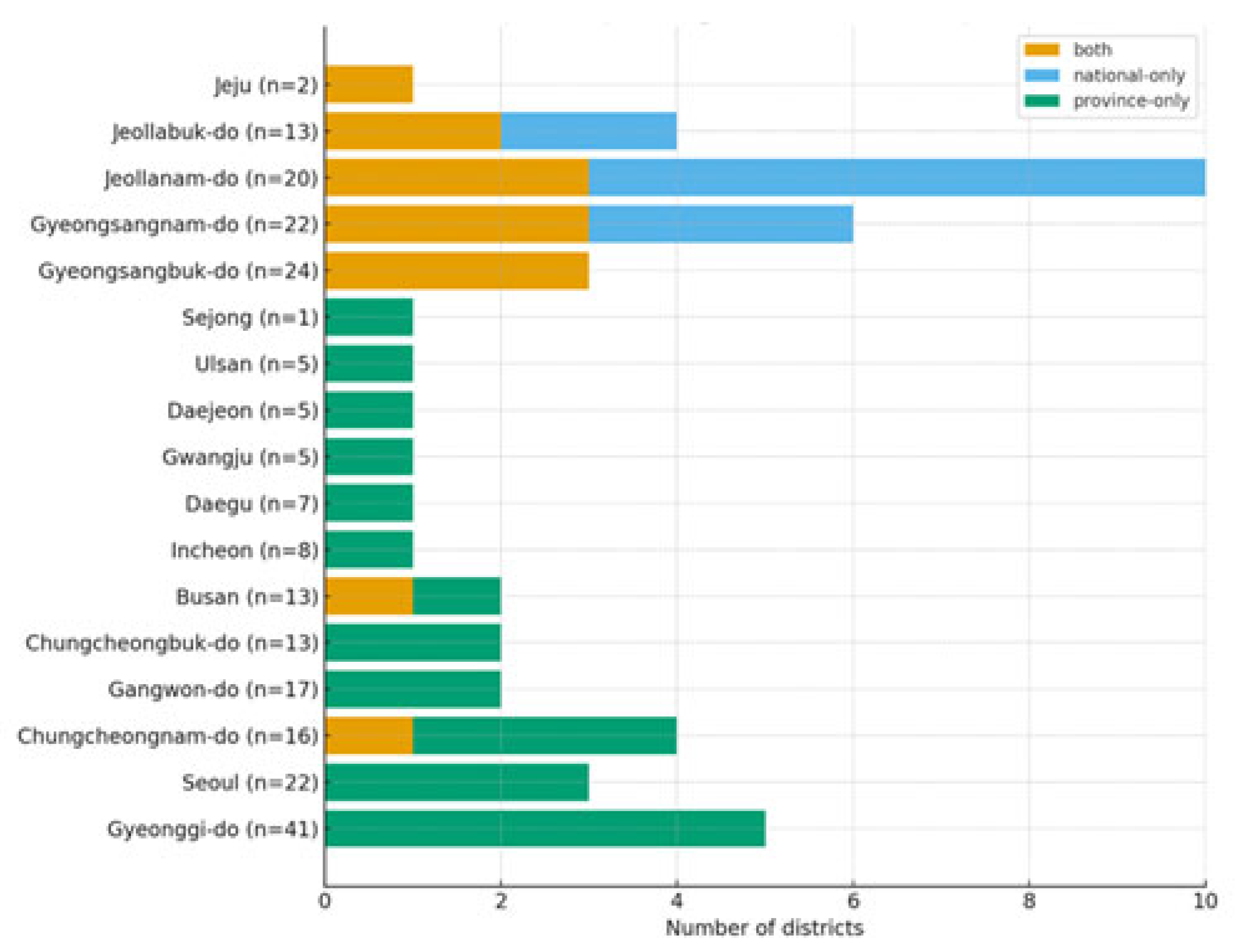
To maintain national comparability while allowing province-level nuance, we apply a dual-cutoff scheme to the same per-district indicator. Specifically, we first compute, for each district, the p95 of per-tree risk under Scenario B (the district-level indicator). We then classify priority status using two p90 cutoffs on that indicator: (i) a national 90th-percentile cutoff (empirical p90 across all districts with ≥1 protected tree), and (ii) a province-specific 90th-percentile cutoff (empirical p90 within each province). Ties at the threshold are included in both cases. Outputs report, for each district, whether it is classified as a priority under the national rule and under the provincial rule, and we flag agreement/disagreement to preserve national comparability while enabling region-tailored targeting. Provinces with very small n are computed but interpreted with caution. No re-estimation of the risk model is performed; only the thresholding rule differs. For visualization, we show counts (both/national-only/province-only) to avoid small-n exaggeration.
2.2.7. Robustness Checks: Weighting Scenarios and Normalization Choices
To ensure that the conclusions of this study are not overly dependent on specific assumptions—such as the choice of weighting schemes or normalization methods—a series of robustness checks was conducted. The common basis for comparison is the ranking of counties according to their mean risk scores. The evaluation proceeds along two dimensions.
First, we assess the effect of changes in weighting scenarios (A/B/C) for heat, rainfall, and species sensitivity on the ranking structure. Second, we examine the impact of switching normalization methods between [0–1] linear normalization and z-standardization on both the composition of the high-risk group and the overall ordering.
For the full set of rankings, stability is consistently summarized by the Spearman rank correlation coefficient (ρ). For the composition of the high-risk group, however, stability is measured differently depending on purpose. Specifically, in the comparison of weighting scenarios, we report the simple retention rate of the top-K group (size of the intersection divided by K). In the comparison of normalization methods, we employ the Top-K Jaccard coefficient, which provides a more conservative and precise measure of compositional agreement. The values of K are standardized at 10, 20, 30, and 50.
- Sensitivity to Weighting Scenario Changes
The three scenarios share identical indicator composition and calculation procedures, differing only in the choice of weights. Accordingly, comparing results across scenarios is equivalent to testing the robustness of the index with respect to weight selection.
For each district, mean risk scores were calculated under each scenario, and the pairwise Spearman correlations (ρ) were computed to evaluate the overall preservation of ranking structure. At the same time, to identify regions relatively sensitive to changes in weights, two supplementary measures were employed: (1) the variance of ranks across the three scenarios, defined as Var (rank A, rank B, rank C) and (2) the total amount of rank movement across scenarios, aggregated as ∣rank A − rank B∣ + ∣rank B − rank C∣ + ∣rank A − rank C∣.
These additional indicators make it possible not only to summarize the degree of stability in aggregate but also to detect particular counties whose relative positions fluctuate most in response to changes in weighting.
- Sensitivity to Normalization Method Changes
To isolate the influence of normalization, we constructed an alternative specification in which the baseline [0–1] linear normalization was replaced entirely with z-standardization. The comparison unit remains the same: district-level rankings of mean risk. For the full distribution of rankings, stability is summarized by Spearman’s ρ, while for the composition of the high-risk group, the Top-K Jaccard coefficient is used.
The Jaccard index is employed here, rather than simple retention rates, for a specific reason. In the case of normalization changes, rescaling of values can generate ties or boundary shifts, leading not only to the entry or exit of counties from the top group but also to reordering within the boundary. As a result, the Jaccard measure—which expresses the intersection relative to the union—serves as a more conservative and sharper diagnostic than simple overlap ratios. In this way, the robustness check captures both membership stability and boundary sensitivity more faithfully.
2.2.8. Boundary Uncertainty via Bootstrap and Fuzzy Boundary
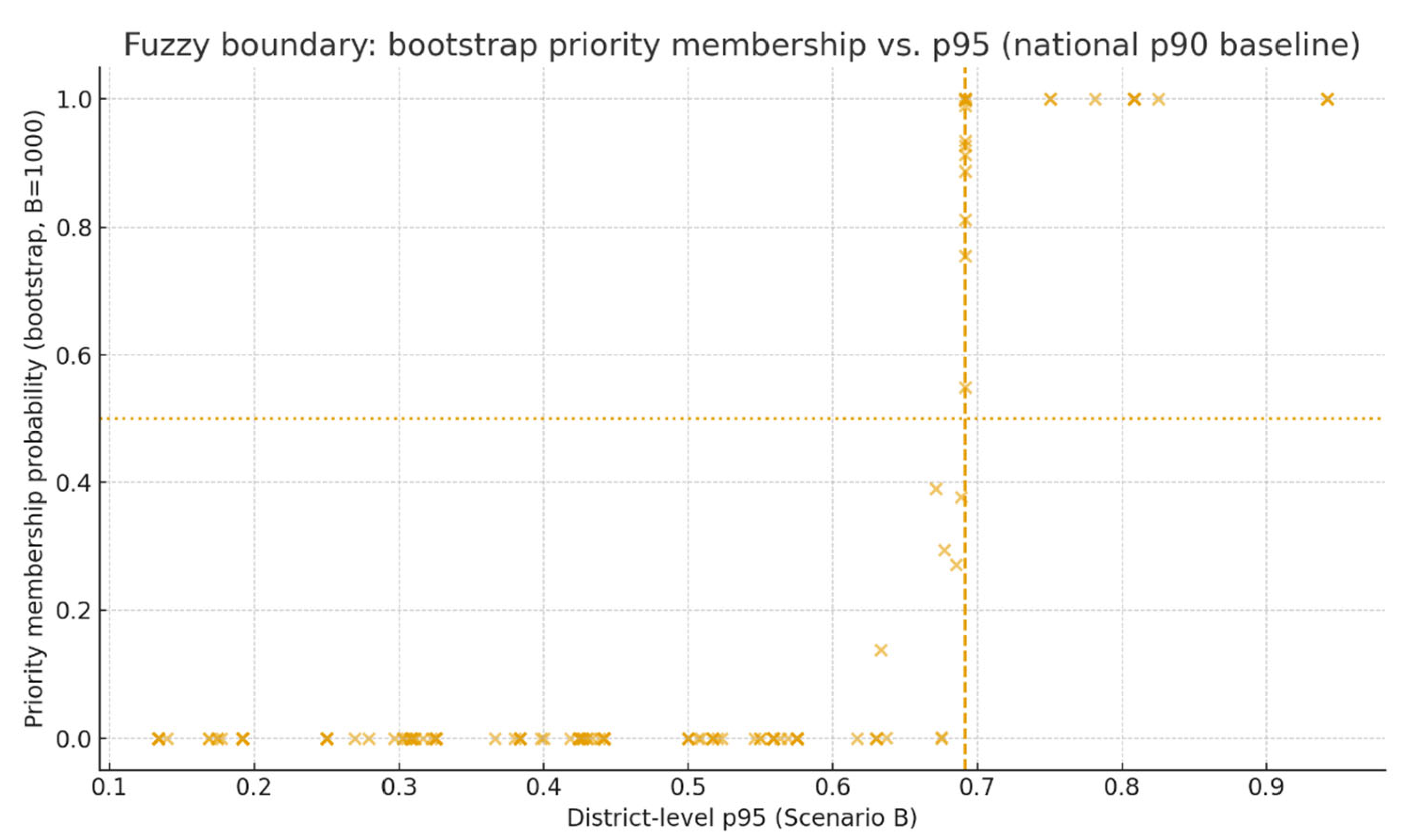
To make the decision boundary explicit, we quantify uncertainty around the national 90th-percentile rule on the same district-level p95 indicator (Scenario B). Each district’s p95 is defined as the 95th percentile of per-tree risk values. Because tail statistics are sensitive to small sample sizes and minor perturbations, we use a nonparametric bootstrap: for each district, we resample trees with replacement and recompute p95 1000 times. On every replicate we also recompute the national 90th-percentile cutoff and record whether the district is classified as priority. The resulting probability of priority status (μ ∈ [0, 1]) is the fraction of replicates in which the district meets the cutoff (higher μ = more robust). We also report 95% confidence intervals for district p95. To identify threshold-sensitive cases, we mark districts that (i) fall within a narrow band around the empirical cutoff (national 90th percentile ±2 percentiles) or (ii) have μ ∈ [0.4, 0.6]. This near-threshold set highlights districts whose priority status is most likely to flip under small changes, without re-estimating the model.
All data analyses and visualizations were conducted in Python (version 3.12.7) using standard scientific libraries (pandas, NumPy, Matplotlib, and GeoPandas).
3. Results
3.1. Descriptive Statistics and Overview of Distributions
3.1.1. Distribution of Protected Tree Individuals and Species Composition
The distribution of protected tree individuals and their species composition provides the background for interpreting subsequent risk assessments. As illustrated in Figure 1, the most frequently occurring species nationwide include Zelkova serrata (zelkova), Celtis sinensis (hackberry), Ginkgo biloba (ginkgo), Pinus densiflora (Korean red pine), and Styphnolobium japonicum (pagoda tree). This pattern reflects both the historical trajectory of designation and regional landscape preferences. Variations in species composition are significant, as they imply that even under identical climatic conditions, differential physiological sensitivities across species can generate heterogeneous responses at the individual risk level. This observation motivates the species-level analysis presented in subsequent sections.
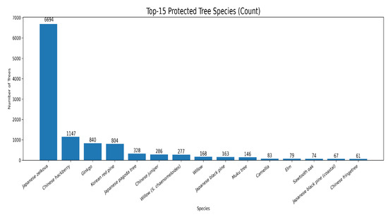
Figure 1.
Top-15 protected tree species (count). Extremely right-skewed; Japanese Zelkova (S01) dominates the inventory, followed by Chinese hackberry (S02). Species mix implies heterogeneous risk response even under similar climate exposure.
3.1.2. Standardization of Indicators onto a Common Scale
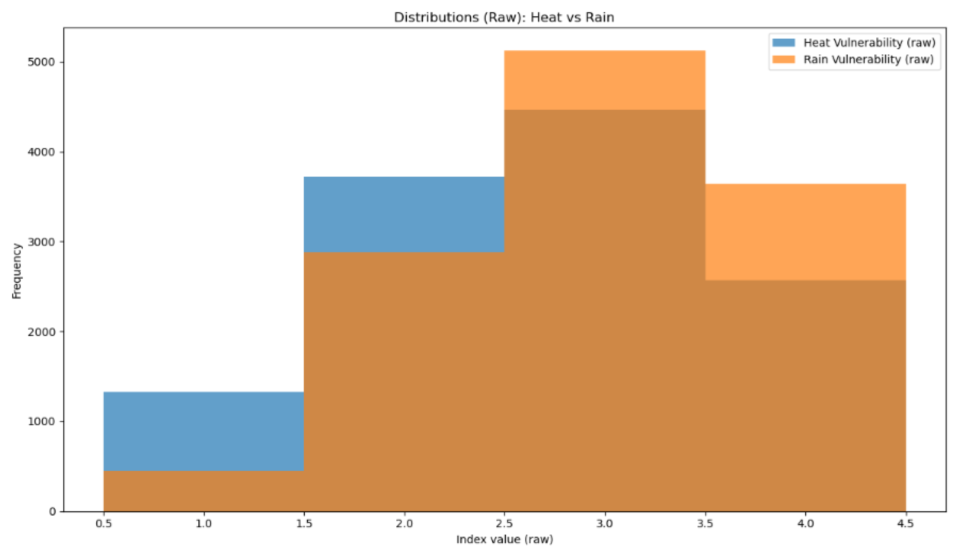
This section demonstrates, using two representative indicators, that normalization preserves the substantive meaning of the original variables. Figure 2 and Figure 3 overlay histograms of the raw and normalized distributions of the heat and rainfall indicators, showing that the transformation does not distort their interpretive content.

Figure 2.
Distributions before min-max normalization (raw indices). The darker brown areas are simply the overlap of the two histograms (alpha = 0.7), not a separate series requiring its own legend. This overlap visually indicates bins where Heat (blue) and Rain (orange) have simultaneously high frequencies.
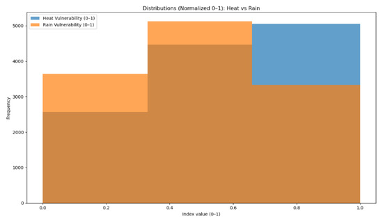
Figure 3.
Distributions after min–max normalization to [0, 1]. Min–max normalization preserves ranks while aligning scales.
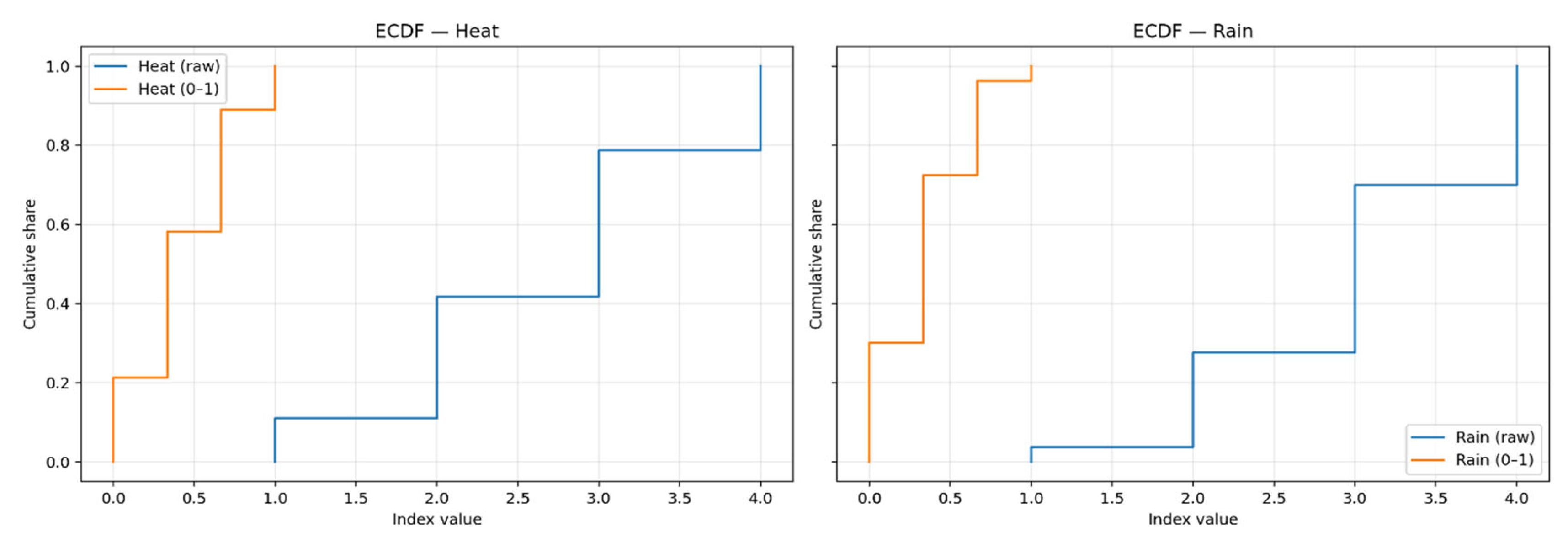
As shown in Figure 3, the exposure indicators for heat and rainfall, as well as species sensitivity scores, were all adjusted to the [0, 1] scale. Missing values and extreme outliers were treated minimally, at a level sufficient to stabilize the tails of the distributions. Nevertheless, under such simple linear normalization, the shapes of the distributions do not change markedly—indeed, this invariance is precisely the reason for applying linear normalization in the first place. To complement the histograms and to provide a clearer visualization of rank preservation, Figure 4 adds overlaid empirical cumulative distribution functions (ECDFs).
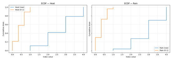
Figure 4.
ECDF (Empirical Cumulative Distribution Function) overlays. These plots allow a visual check of how the positions of tail segments (e.g., the top 10%) in the original data correspond to those in the normalized [0, 1] scale.
To numerically verify how identical percentiles in the raw and normalized scales correspond to one another, Table 4 presents tail mass and percentile statistics.

Table 4.
Tail mass and percentile summary. The table reports 50th percentile, 90th percentile, and 99th percentile, the proportion of individuals in the top 10% (raw scale vs. 0–1 scale), and skewness. Because normalization is intended to adjust scales rather than alter distributional shape, skewness is generally preserved before and after normalization. Indeed, the table confirms that the distribution of individual-level risk values retains a similar skewness pattern after normalization.
As shown in Figure 4 and Table 4, the top 10% set in the raw scale corresponds one-to-one with the ≥0.9 segment in the normalized scale. This confirms that percentile-based thresholds can be interpreted consistently on the [0, 1] axis, and that indicators on different scales can be compared on a unified scale without distortion. Taken together, these findings demonstrate that, after [0, 1] linear normalization, the median and upper percentiles of the heat and rainfall exposure indicators continue to reflect the same ranking order as in the raw scale. At the same time, the original distributions of heat and rainfall vulnerability are observed to have right-skewed tails, and the presence of these high-risk tails is preserved even after normalization. For this reason, subsequent aggregation at the regional level consistently reports not only mean values but also upper-tail proportions.
3.2. National, Provincial, and District-Level Risk Landscapes
This section examines the configuration of risk at national and regional scales. Using Scenario B as the baseline, the analysis first presents an overview of mean risk nationwide in the form of a map. This is followed by inter-provincial comparisons to highlight broader macro-regional differences. Next, the analysis turns to district-level patterns under Scenario B, reporting more detailed numerical values. Finally, across all scenarios, those counties that consistently rank among the highest-risk districts are identified and compared.
3.2.1. National Risk Map (Based on Scenario B)
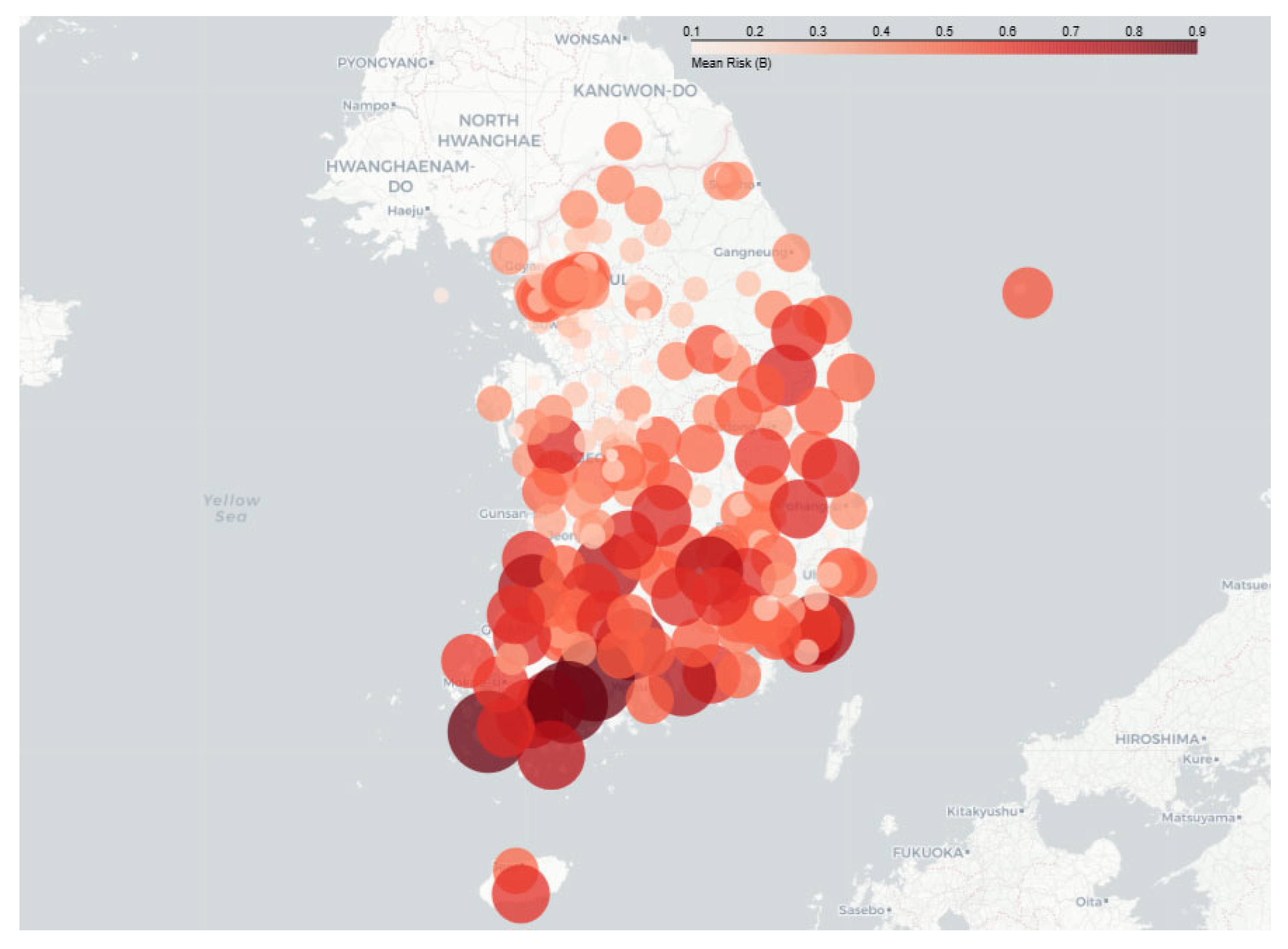
When the composite risk index is visualized at the district level using Scenario B, a distinctive high-risk belt emerges, concentrated along the southern coast and the southwestern region, as shown in Figure 5. Metropolitan areas, by contrast, tend to exhibit relatively lower levels of risk or heterogeneous, localized patterns. In addition, several isolated high-risk pockets are also observed in inland mountainous areas.
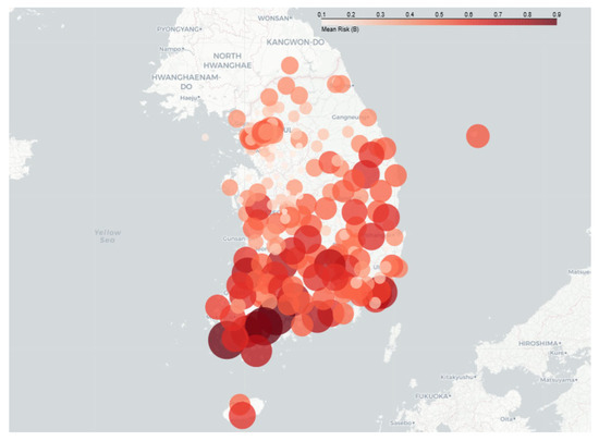
Figure 5.
National mean risk map under Scenario B (kNN = 8, permutations = 199, p < 0.05). Statistically significant clusters are observed in the southwestern region and in certain inland mountainous areas.
This map should be interpreted as a relative assessment: it does not, by itself, determine the specific causes of risk. Rather, it serves as a signal indicating where priority monitoring and inspections should be directed, and where resources and personnel may most effectively be allocated.
3.2.2. Provincial-Level Comparison
(Throughout this subsection, “provincial mean risk” refers to a regional indicator aggregated stepwise from individual protected trees to counties and then to provinces. Thus, the values are attached not to individual species or trees but to regions, reflecting both the climatic exposures to heat and rainfall and the species composition, i.e., the distribution of sensitivities, in each province).
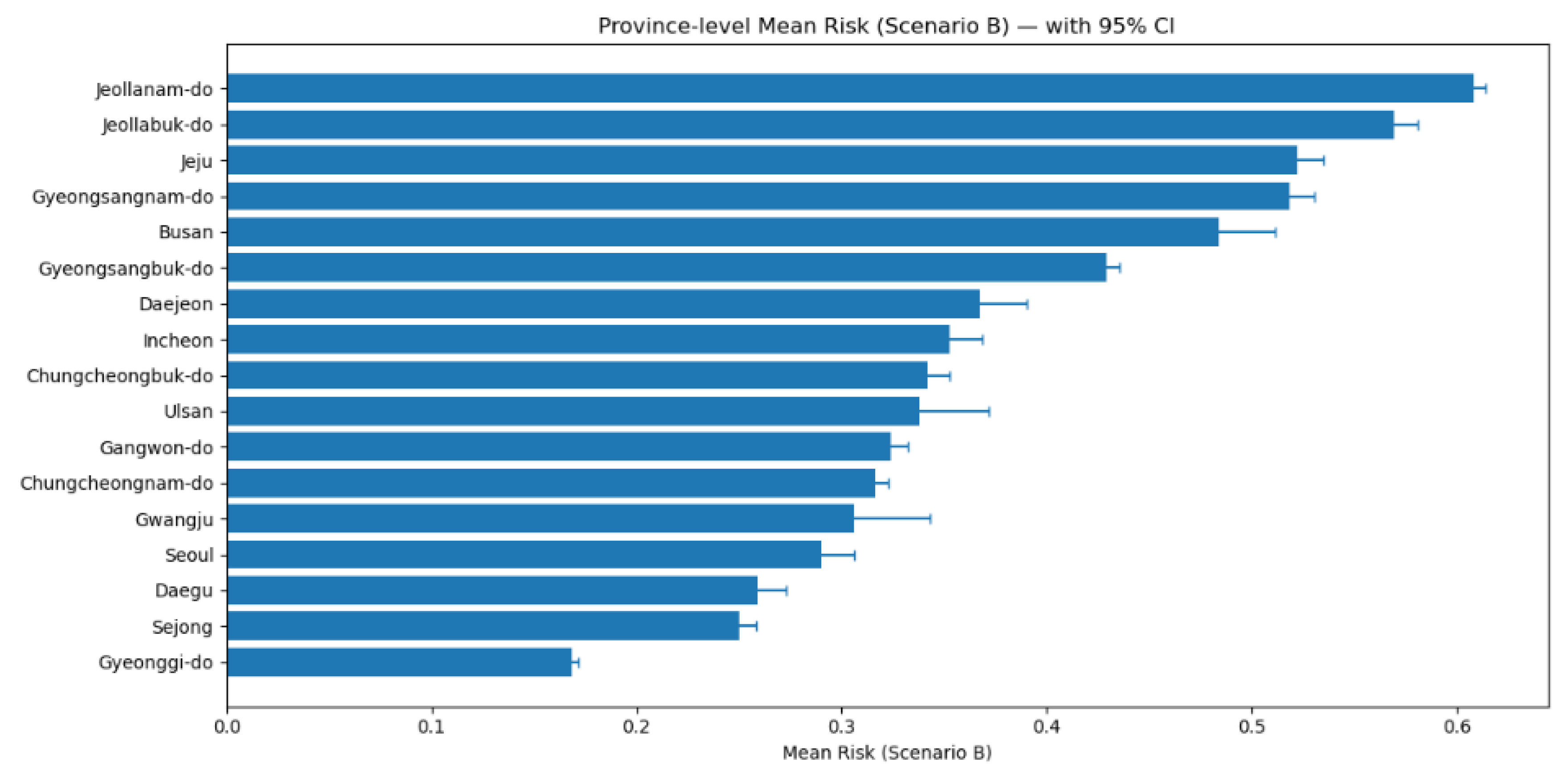
At the provincial level, mean risk exhibits a pronounced spatial gradient. As illustrated in Figure 6, Jeollanam-do and Jeollabuk-do consistently record the highest mean risks, remaining significantly above all other provinces even when confidence intervals are considered. Next in rank is a group consisting of Gyeongsangnam-do, Jeju, Busan, and Gyeongsangbuk-do, followed by the mid-range group of the Chungcheong region, Gangwon, and Incheon. By contrast, the major metropolitan areas—Seoul, Gyeonggi, Daegu, and Sejong—exhibit relatively lower values.
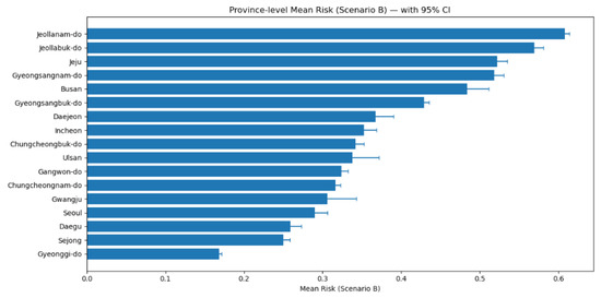
Figure 6.
Provincial-level mean risk (Scenario B, 95% CI). Horizontal axis shows provincial means with 95% confidence intervals. Jeollanam-do, Jeollabuk-do, and Gyeongsangnam-do occupy the highest ranks, while metropolitan areas exhibit comparatively low values.
This pattern can be interpreted as the combined outcome of (i) greater rainfall vulnerability in the southern coastal zones and (ii) the prevalence of species particularly sensitive to flooding and heat stress in those same regions. Although the 95% confidence intervals for some provinces overlap, the superiority of Jeollanam-do and Jeollabuk-do is evident, with differences that extend beyond the overlap ranges.
These differences in mean risk are also reflected in the summary tables (Table 5 and Table 6) below.

Table 5.
Provincial summary (Scenarios A/B/C: mean, standard error, Δrank). Provincial means, standard errors, and rank-order tables.

Table 6.
Provincial summary (Top 15 provinces by mean risk under Scenario B; wH = 0.35, wR = 0.4, wS = 0.25). Same format as Table 5.
3.2.3. Mean Risk Under Scenario B
When counties are ranked by mean risk and by upper percentiles (e.g., p95) under Scenario B, a consistent set of core candidates emerges, including Jangheung, Jindo, Boseong, and Hadong. In other words, Jeollanam-do, Jeollabuk-do, and Gyeongsangnam-do are repeatedly found at the top of the rankings, with Jangheung, Jindo, and Boseong serving as “apex” counties that score high on both mean and p95 indicators (See Table 7 and Table 8 below).

Table 7.
Top 20 counties by mean risk under Scenario B (wH = 0.35, wR = 0.4, wS = 0.25).

Table 8.
Top 20 counties by p95 risk under Scenario B (wH = 0.35, wR = 0.4, wS = 0.25). These figures highlight the upper-tail distribution of risk. Unlike simple averages, the p95 criterion identifies which regions should be prioritized for management when the focus is on extreme events such as sustained heat waves or localized heavy rainfall.
As discussed in more detail below, the Top-20 list of mean risk and the High–High clusters identified by LISA did not overlap, as the two capture different measurement concepts: LISA reflects spatial clustering, whereas the Top-20 list highlights absolute risk levels. From a management perspective, the two criteria can thus be regarded as complementary in setting conservation priorities.
3.2.4. Counties Consistently Ranked at the Top Across All Scenarios
How do results change under alternative scenarios? When considering the intersection of the Top 20 counties across Scenarios A, B, and C, a consistent set emerges that includes Jangheung, Jindo, and Boseong (Jeollanam-do), Hadong and Namhae (Gyeongsangnam-do), and Gochang and Imsil (Jeollabuk-do) (see Table 7, Table 8 and Table 9).

Table 9.
Intersection of Top 20 counties across Scenarios A, B, and C (based on both mean and p95 rankings).
At the same time, comparison of the Top 20 counties by mean risk across Scenarios A, B, and C reveals a repeated set including Jangheung, Jindo, and Boseong (Jeollanam-do), Hadong and Namhae (Gyeongsangnam-do), Gochang and Imsil (Jeollabuk-do), as well as Haenam and Wando (Jeollanam-do). This consistency indicates that even when the emphasis among weights shifts, the top ranks remain largely unchanged, underscoring the robustness of the highest tier. In particular, the southern coast and southwestern inland regions form a persistent high-risk zone, shaped by the combined influence of heat and rainfall vulnerabilities together with the composition of species highly sensitive to these stresses.
By contrast, counties such as Sunchang and Buan (Jeollabuk-do) or Uiseong (Gyeongsangbuk-do) appear in the Top 20 under only two of the scenarios. These are interpreted as boundary cases, whose rankings shift modestly depending on whether greater weight is given to species sensitivity or other factors.
Inspection of Table 10 shows that heat (H) is the dominant driver in most repeatedly included counties, such as Hadong, Namhae, Gochang, and Imsil. Rainfall (R) plays a leading role in certain lowland or coastal areas, exemplified by Suyeong-gu (Busan) and Gangjin (Jeollanam-do). In some cases, multiple factors operate at comparable magnitudes, producing a “Mixed” classification. Notably, even among counties appearing in all three scenarios (e.g., Jangheung, Jindo, Boseong in Jeollanam-do, and Bonghwa in Gyeongsangbuk-do), several are categorized as Mixed. This indicates the presence of compound risk, requiring simultaneous attention to heat, rainfall, and species management.

Table 10.
Scenario-specific Top 20 counties. driver_this_scenario indicates the dominant factor in a given district under the specified scenario (A, B, or C). driver_mode_across_selected denotes the modal dominant factor across all scenarios in which the district appears. ‘Scenarios included’ specifies the number of scenarios (0–3) in which the district is included in the Top 20. For example, a value of 3 indicates that the district appears under all three scenarios, suggesting a robust high-risk status independent of weighting assumptions.
From a practical standpoint, it is reasonable to propose the following prioritization: counties included in all three scenarios (3/3) form the first-tier inspection group; those included twice (2/3) constitute the second tier, to be conditionally prioritized; and those appearing once (1/3) are treated as third-tier candidates, to be considered in light of additional contextual information.
3.3. Species-Specific Patterns and Cross-Regional Interactions
3.3.1. Species-Specific Patterns
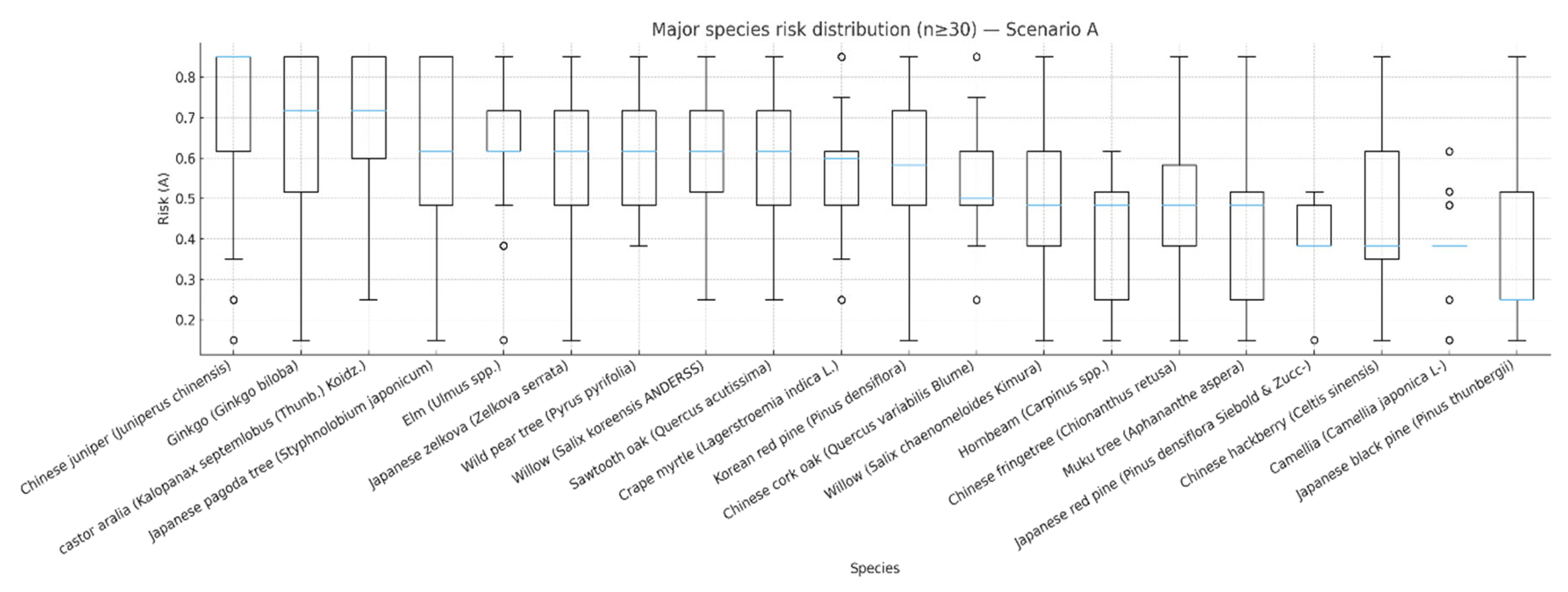
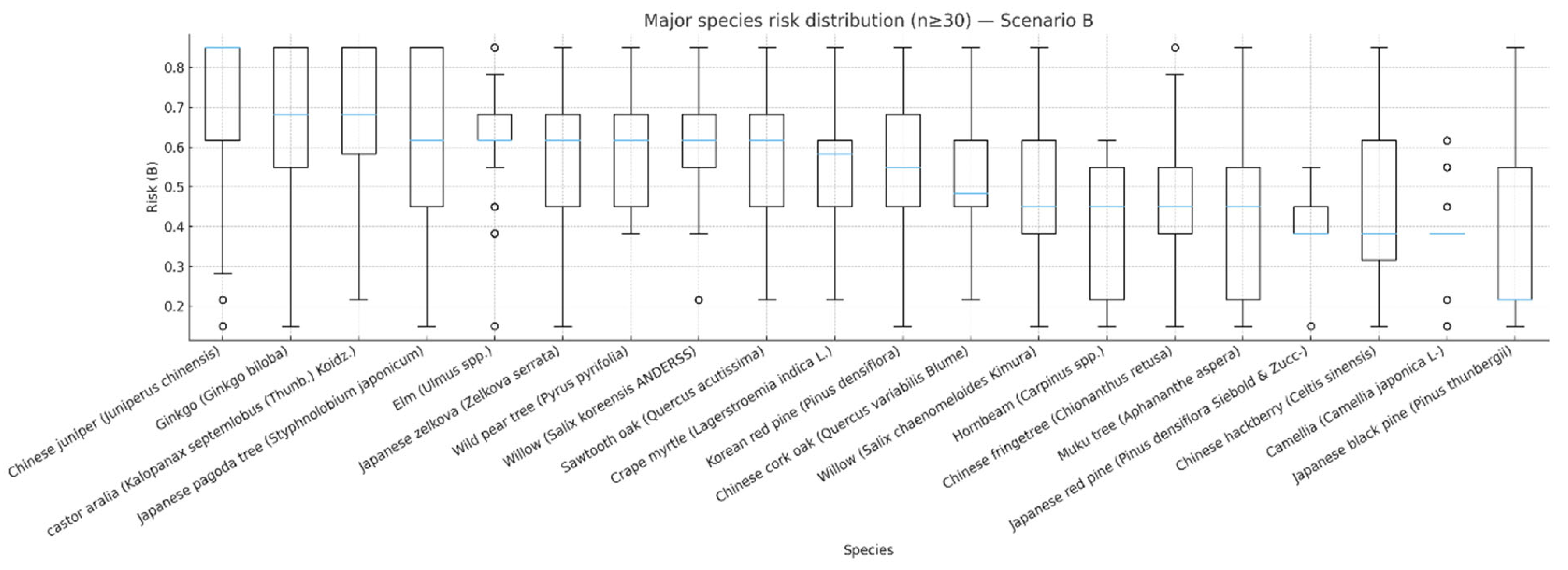
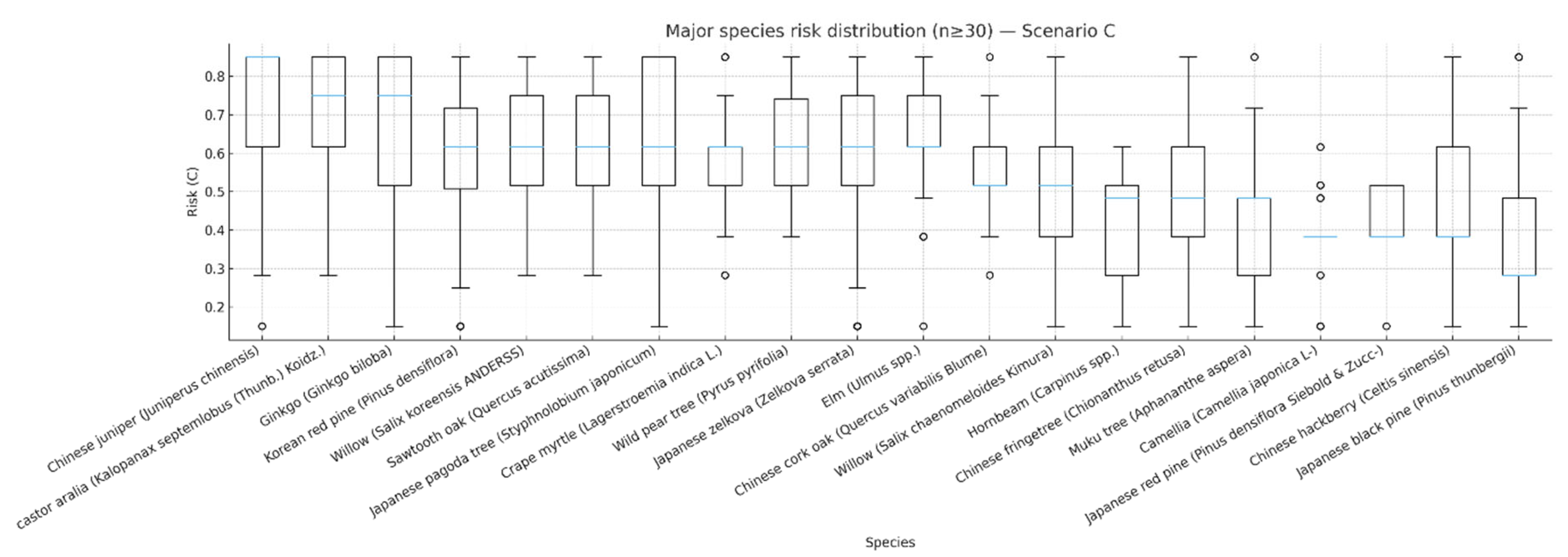
We begin by examining several major species with sample sizes of at least 30 individuals, in order to identify species-specific vulnerabilities reflected in the distribution of risk scores. As illustrated in Figure 7, Figure 8 and Figure 9, the boxes represent interquartile ranges (IQR), the central lines denote medians, and whiskers are drawn using the 1.5 × IQR rule. Species with higher overall risk levels show elevated medians and thicker upper tails. The clear differences in medians and dispersions across species confirm the presence of species-specific vulnerabilities. For species with large variance, management carries greater uncertainty, while for those with smaller variance, risk management is relatively more predictable.
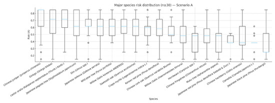
Figure 7.
Distribution of risk scores for major species under Scenario A (n ≥ 30). The absence of a box indicates that the data for this species have little variation or too few observations to form an interquartile range. The blue line marks the median, and the circles denote outliers.
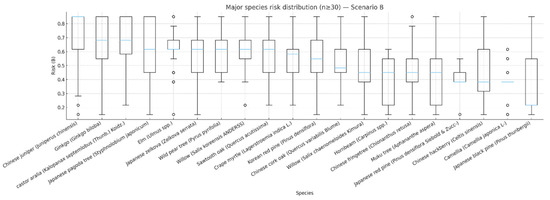
Figure 8.
Distribution of risk scores for major species under Scenario B (n ≥ 30). While relative rankings are largely preserved across scenarios, species sensitive to rainfall exhibit slightly higher medians and thicker upper tails under Scenario B compared to Scenario A. Please refer to the explanation in Figure 7 for the meaning of the absence of a box.
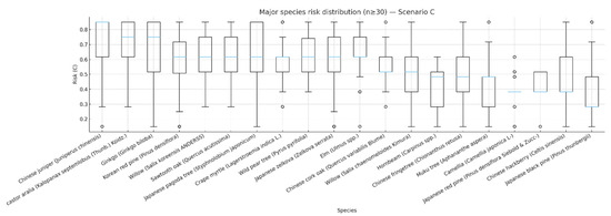
Figure 9.
Distribution of risk scores for major species under Scenario C (n ≥ 30). For some heat-sensitive species, medians are relatively higher than under Scenario A, and variance is enlarged in certain cases. Please refer to the explanation in Figure 7 for the meaning of the absence of a box.
Table 11 summarizes the risk profiles of major species under each scenario, numerically confirming the patterns observed in Figure 7, Figure 8 and Figure 9. Here, n denotes the sample size; smaller sample sizes warrant more cautious interpretation. The mean and standard deviation capture overall levels and variability, while top10_X (for each scenario X) indicates the proportion of individuals in the top 10% of risk scores—that is, the thickness of the high-risk tail.

Table 11.
Species-level summary of major species (n ≥ 30) across Scenarios A, B, and C. Includes sample size, mean, standard deviation, and proportion in the top 10% for each scenario. Relative rankings are generally stable across scenarios, though certain species exhibit more pronounced high-risk tails.
For instance, Zelkova serrata (zelkova) shows high mean scores across all three scenarios (0.58–0.60) with a top 10% proportion of about 0.18. Juniperus chinensis (Chinese juniper) records not only high mean values but also a very thick high-risk tail (top 10% ≈ 0.58). By contrast, Pinus thunbergii (black pine) exhibits both a lower mean and smaller variance (top 10% ≈ 0.01), positioning it closer to the low-risk group. These top 10 indicators provide practical implications, as they suggest the actual intensity of on-the-ground risk management required.
In addition, Table 12 aggregates the species-sensitivity label combinations (heat/flood) of only those protected trees that fall above the 90th-percentile risk threshold, within the counties that consistently appear in the Top 20 across Scenarios A, B, and C.

Table 12.
Distribution of sensitivity labels (heat vs. flood) for high-risk individuals (≥90th percentile) in species located within the Top 20 counties common to all three scenarios.
As revealed in Table 12, when focusing exclusively on those high-risk individuals (≥90th percentile) within the counties that consistently rank in the Top 20 across all scenarios, a common pattern emerges irrespective of scenario: these individuals tend to be strong against heat but vulnerable to rainfall/flooding. The predominance of the “heat-resistant but flood-sensitive” combination has important implications, as it directly informs which management strategies should be prioritized for effective policy design.
3.3.2. Cross-Analysis of Species and Regions
Across Scenarios A, B, and C, a total of 37 counties are consistently classified as hot spots (HH). When species are cross-tabulated with regions under Scenario B, the leading species in these high-risk counties can be identified (see Table 13). For consistency, the analysis is restricted to major species with sufficient sample sizes (n ≥ 30).

Table 13.
Differences in species-level median risk values within counties that are hot spots (HH) across all three scenarios (A, B, C). Here, n_nat denotes the number of individuals of the species nationwide, while n_hot is the number of individuals of that species located within counties that are consistently HH across scenarios. The table reports the median risk within the hot-spot set (med_hot) and compares it with the nationwide median (med_nat), with the difference expressed as Δmed. This allows identification of species that are disproportionately elevated in high-risk areas.
Species-level medians within the HH counties common to Scenarios A, B, and C are significantly higher than the corresponding nationwide medians. For example, Ginkgo biloba shows a median increase of +0.38, Juniperus chinensis +0.37, Pinus densiflora +0.25, and Zelkova serrata +0.23. To illustrate, the row for Ginkgo biloba can be read as follows: nationwide, there are 840 individuals of this species with a median risk of 0.25; within the HH counties common to all three scenarios, there are 70 such trees, whose median risk rises to 0.6333, representing a difference of +0.3833 compared to the nationwide level.
3.4. Decomposition of Vulnerability Components in Key Regions and Policy Prioritization
3.4.1. Decomposition of Vulnerability Components in Key Regions
Table 14 presents a decomposition of average risk components for counties that consistently appear in the Top 20 across all three scenarios (A, B, C). These counties were first identified by extracting the Top 20 under each scenario and then intersecting the sets.

Table 14.
Component decomposition summary of counties included in the Top 20 across all scenarios (based on mean risk). Includes normalized values for heat, rainfall, and species sensitivity components.
This table illustrates whether a given district is predominantly “heat-driven,” “rainfall-driven,” or characterized by particular species sensitivities (heat/flood). In doing so, it captures the relative configurations of high heat vulnerability, high rainfall vulnerability, and species-specific sensitivities. These distinctions can be directly translated into policy prescriptions. For example, decomposition of several specific counties shows that Hadong and Namhae are primarily heat-vulnerable, while Boseong, Jangheung, and Jindo exhibit combined high vulnerabilities to both heat and rainfall. In the latter case, effective interventions must integrate both types of measures—such as shading, ventilation, and soil depth improvements for heat mitigation, alongside drainage and permeable pavements to alleviate rainfall-related risks.
3.4.2. Policy and Priority Lists
For practical application, a policy priority list was generated under Scenario B by adopting the global 90th-percentile threshold (q = 0.90) as the criterion (see Table 15). For each district, the table records the number and proportion of individuals exceeding the threshold, the dominant species sensitivity label (heat/rain), the representative species list (top three species), and the corresponding recommended interventions.

Table 15.
Policy and priority list based on Scenario B (90th-percentile threshold applied nationwide). In the recommendation field, X refers to “drainage channel maintenance/permeable paving and rain gardens/securing soil depth/improving root respiration of flood-sensitive species (through soil aeration and mounding)”, while Y refers to “providing shade/installing shade nets and managing evapotranspiration (e.g., mulching)/optimizing irrigation schedules/protecting trunks with reflective coatings/monitoring soil moisture.”
By jointly presenting both the rationale (“why this district should be prioritized”) and the corresponding action plan (“what should be done once prioritized”), the table provides an immediate and actionable basis for the selection of management priorities and the formulation of implementation strategies. For conciseness, only the top 30 counties are reported here.
Recommended measures are listed for the top counties, with treatments tailored to the specific vulnerabilities observed. For example, in counties with a high prevalence of rainfall-sensitive species, prescriptions emphasizing drainage, soil depth, and permeable infrastructure are repeatedly proposed. Although general maintenance measures—such as sustaining tree vigor, controlling pests and diseases, and maintaining soil fertility—were available, these high-risk areas were not recommended for such generic prescriptions, given their elevated risk levels.
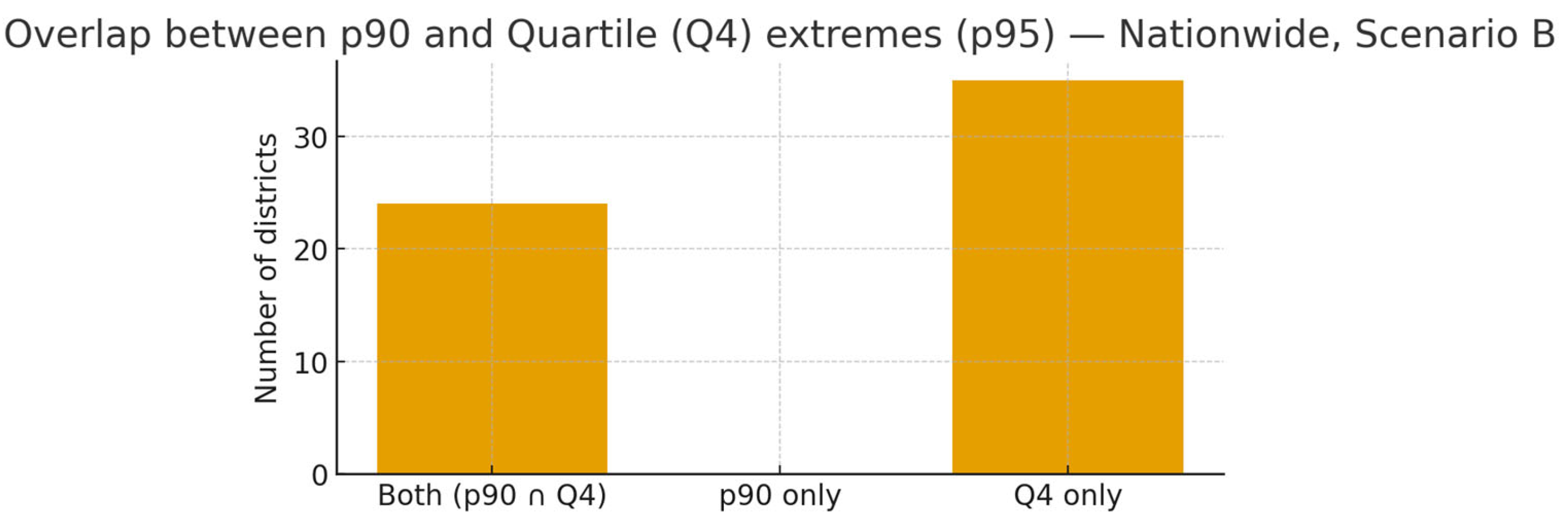
Using quartiles as an alternative extreme definition on the district-level p95 indicator yields a broader but still consistent picture relative to the p90 rule. Under the national p90 threshold (p95 ≥ 0.9234), the top decile of districts is classified as extreme (n = 24), reflecting a conservative notion of the tail. By contrast, the quartile rule (Q4, p95 ≥ 0.8290) admits a wider slice (n = 59) and fully contains the p90 set (intersection = 24; p90-only = 0; Q4-only = 35; Jaccard = 0.407). In practical terms, p90 pinpoints the very highest-risk cases, whereas Q4 expands the candidate pool by adding mid-tail districts for screening (Figure 10; Table 16). All thresholds come from the national distribution with ties included.
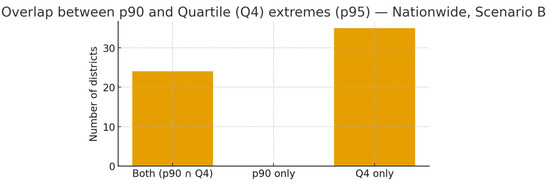
Figure 10.
Overlap between p90 (top decile) and quartile (Q4, top quartile) extremes on district-level p95 (Scenario B). A simple overlap view shows that the p90 extreme set is fully nested within the Q4 set: p90 provides a conservative tail while Q4 broadens coverage to the mid-tail. Thresholds are computed on the national distribution (ties included).

Table 16.
Extreme-risk membership by definition (p90 vs. Q4) on district-level p95 (Scenario B). Under the national p90 rule (top decile), districts with p95 ≥ 0.9234 are classified as extreme (n = 24). Under the quartile rule (Q4, top quartile), districts with p95 ≥ 0.8290 are classified as extreme (n = 59). Q4 fully contains p90 (intersection = 24; p90-only = 0; Q4-only = 35; Jaccard = 0.407). The table lists members only (both/Q4-only), ordered by p95. All thresholds are based on the national distribution (ties included). The analysis covers 234 districts with ≥1 protected tree.
Using identical p95 values, we compare the national 90th percentile (baseline, cross-region comparability) with the province-specific 90th percentile (within-province targeting). The pattern is consistent: the national rule preserves a stable priority core, whereas province-specific thresholds add a small province-only set at the margins, most visibly in provinces with higher within-province dispersion (cf. CV/IQR). We present the number of districts in each category (both/national-only/province-only) by province to avoid small-n distortion (Figure 11). A province-level summary table reports agreement rate (share of districts where the two rules agree, i.e., both priority or both non-priority) and dispersion indicators (Table 17). All thresholds include ties; only districts with ≥1 protected tree are considered.

Figure 11.
National vs. province-specific 90th percentile on district-level 95th percentile (Scenario B)—counts. Each row is a province (labeled with n), and the bar length shows the number of districts (not shares). Orange (“both”) are districts classified as priority by both rules and therefore indicate the size of the priority core; blue (“national-only”) are districts priority by the national rule but not by the province rule, indicating cases that look extreme nationally but are not top-decile within their own province; green (“province-only”) are districts priority only under the province rule, i.e., additional screening workload that emerges when within-province thresholds are used. Practically, a long orange segment means strong agreement and a sizable core; a long green segment means province-specific thresholds add many margin cases and are therefore most informative in that province (often where within-province dispersion is higher). A long blue segment suggests districts that rank high nationally but not within their province, informing potential re-prioritization at the provincial level.

Table 17.
Province-level comparison of national vs. province-specific 90th-percentile thresholds (district p95, Scenario B)—counts. For each province (labeled with n), we report the number of districts classified as priority by both rules, national-only, and province-only, together with the agreement rate (share of districts where the two rules agree: both priority or both non-priority) and dispersion indicators (CV/IQR). Using counts avoids small-n exaggeration (e.g., Sejong n = 1; Jeju n = 2).
A national 90th-percentile cutoff is essential for comparability across regions and time. Yet provinces differ in climate and management capacity; consistent with our dispersion findings, the province-specific 90th percentile is most informative in high-dispersion provinces, where it broadens screening without overturning the national priority core. In low-dispersion provinces, province-specific thresholds bring little change, so the national rule alone generally suffices
3.5. Spatial Patterns and Visualization of Risk
3.5.1. Spatial Autocorrelation and Clusters (LISA)
As noted earlier, this study defines neighbors using district centroids with a k-nearest neighbors (kNN) structure, where k = 8 serves as the baseline. Based on this definition, the global Moran’s I was computed and revealed a statistically significant positive autocorrelation. Specifically, under Scenario B, Moran’s I was estimated at 0.476 (p ≈ 0.001, permutations = 999, k = 8). A value of I = 0.476 indicates moderate-to-strong positive spatial autocorrelation, meaning that neighboring counties tend to have more similar mean risk values than would be expected under spatial randomness. This result statistically corroborates the visual patterns observed in Section 4.2, namely that high-risk areas exhibit clustering rather than random dispersion.
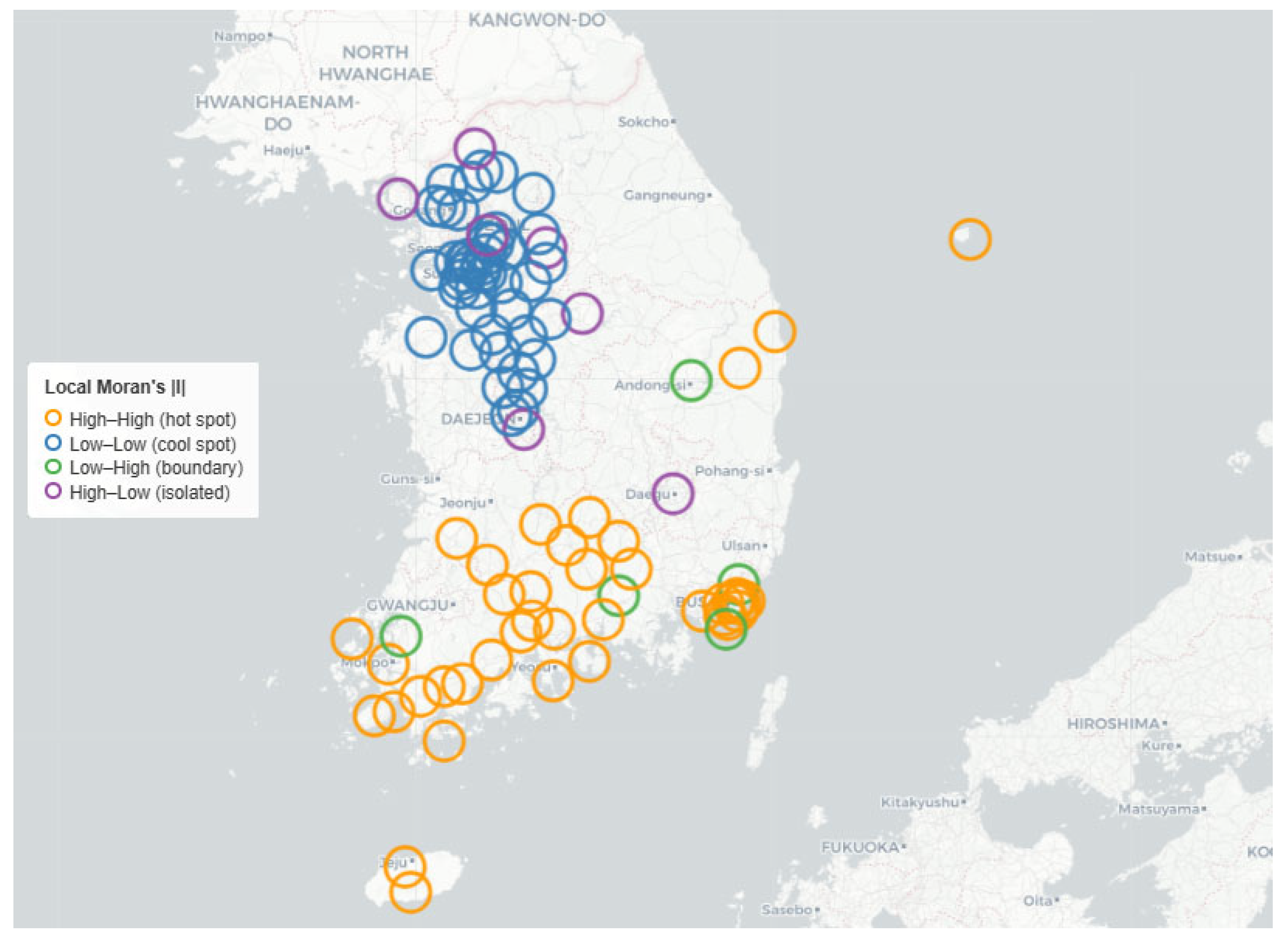
Figure 12 presents the results of LISA analysis with the mean risk layer removed (i.e., with the mean-risk layer turned off), showing only LISA outcomes. Hot spots (HH) are evident in the southern coastal regions, Jeju, and Busan. In the visualization, regardless of color palette, each circle marks a statistically significant LISA location (p < 0.05), with only the type and position of cluster emphasized. Orange indicates high-risk counties clustered with high-risk neighbors (High–High hot spots). Blue indicates low-risk counties clustered with low-risk neighbors (Low–Low cool spots). Green indicates boundary zones where low-risk counties are surrounded by high-risk neighbors (Low–High). Purple indicates isolated zones where high-risk counties are surrounded by low-risk neighbors (High–Low). This representation makes it possible to clearly identify where hot spots cluster in particular regions, and where boundary or isolated zones (Low–High, High–Low) are distributed.
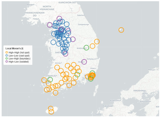
Figure 12.
Spatial patterns indicated by LISA under Scenario B. Multiple regional clusters are shown in distinct colors. Concentrated HH clusters are observed in much of Jeollanam-do and parts of Gyeongsangnam-do (including Hadong, Namhae, and Hapcheon).
Numerical results provide further detail. Under Scenario B, the number of statistically significant Local Moran’s I points (p < 0.05) totaled 93, distributed across categories as follows: 40 HH, 5 LH, 42 LL, and 6 HL. The top 30 counties identified by LISA are summarized in Table 18.

Table 18.
Summary of Local Moran’s I (a form of LISA) under Scenario B. mean_r indicates the mean risk in Scenario B for each district. local_I is the Local Moran’s I statistic, representing the degree to which a district’s value moves in tandem with its neighbors (higher values indicate stronger similarity, such as “I am high and my neighbors are also high”). p_local reports the p-values of Local Moran’s I obtained through permutation tests (two-sided). Significance is set at p < 0.05, based on 999 permutations.
Figure 13 overlays district-level mean risks with significant LISA High–High clusters. Mean risk is represented by bubble size and color, while significant High–High clusters are shown as hollow outlines. This dual visualization enables simultaneous interpretation of both “where risk is high” and “whether high risk is spatially connected.”
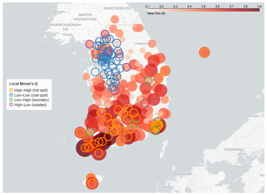
Figure 13.
National composite risk map under Scenario B. District-level mean risks (bubbles) are partially overlain with outlines of LISA High–High clusters (k = 8, permutations = 199, p < 0.05). Significant clustering is observed in the southwestern region and certain inland mountainous areas.
3.5.2. Sensitivity of Spatial Autocorrelation to Neighbor Definitions
At the national scale, spatial autocorrelation proved robust to alternative neighbor definitions. As shown in Table 19, when the number of kNN neighbors was varied from 6 to 12, the global Moran’s I remained statistically significant (p = 0.001) across all specifications, ranging from 0.494 (k = 6) to 0.414 (k = 12). The HH (39 counties) and LL (43 counties) clusters identified under the baseline k = 8 were largely reproduced at other values of k. In other words, district-level mean risk consistently displayed strong positive spatial clustering regardless of the choice of neighbor definition, while the slight decline in Moran’s I as k increased reflected the typical pattern of greater spatial smoothing when larger neighborhoods are used.

Table 19.
LISA neighbor sensitivity summary (α = 0.05, permutations = 999, Scenario B). n_sig indicates the number of significant LISA locations; HH, LH, LL, and HL refer to the counts of significant clusters by type. global_I and global_p denote the global Moran’s I and its significance level, respectively. jaccard_vs_k8 reports the Jaccard similarity of HH/LL locations compared with the baseline k = 8.
Relative to the baseline (k = 8), the Jaccard similarity for HH clusters was very high, ranging from 0.86 to 0.97 for k = 6–10, and remaining high at 0.70 even for k = 12. For LL clusters, Jaccard similarity was similarly high, ranging from 0.83 to 1.00 for k = 6–10, and still 0.77 at k = 12. This confirms that the positions of the core HH and LL clusters are highly robust, with changes in k leading only to minor local adjustments along the boundaries.
The number of significant LISA locations increased from 90 (k = 6) to 120 (k = 12), displaying the expected pattern of enhanced statistical power with neighborhood expansion. Since larger k values incorporate more neighbors, the increased detection of significant clusters under higher k values is a natural outcome.
3.5.3. Quantifying Spatial Inequality of Risk Across Provinces
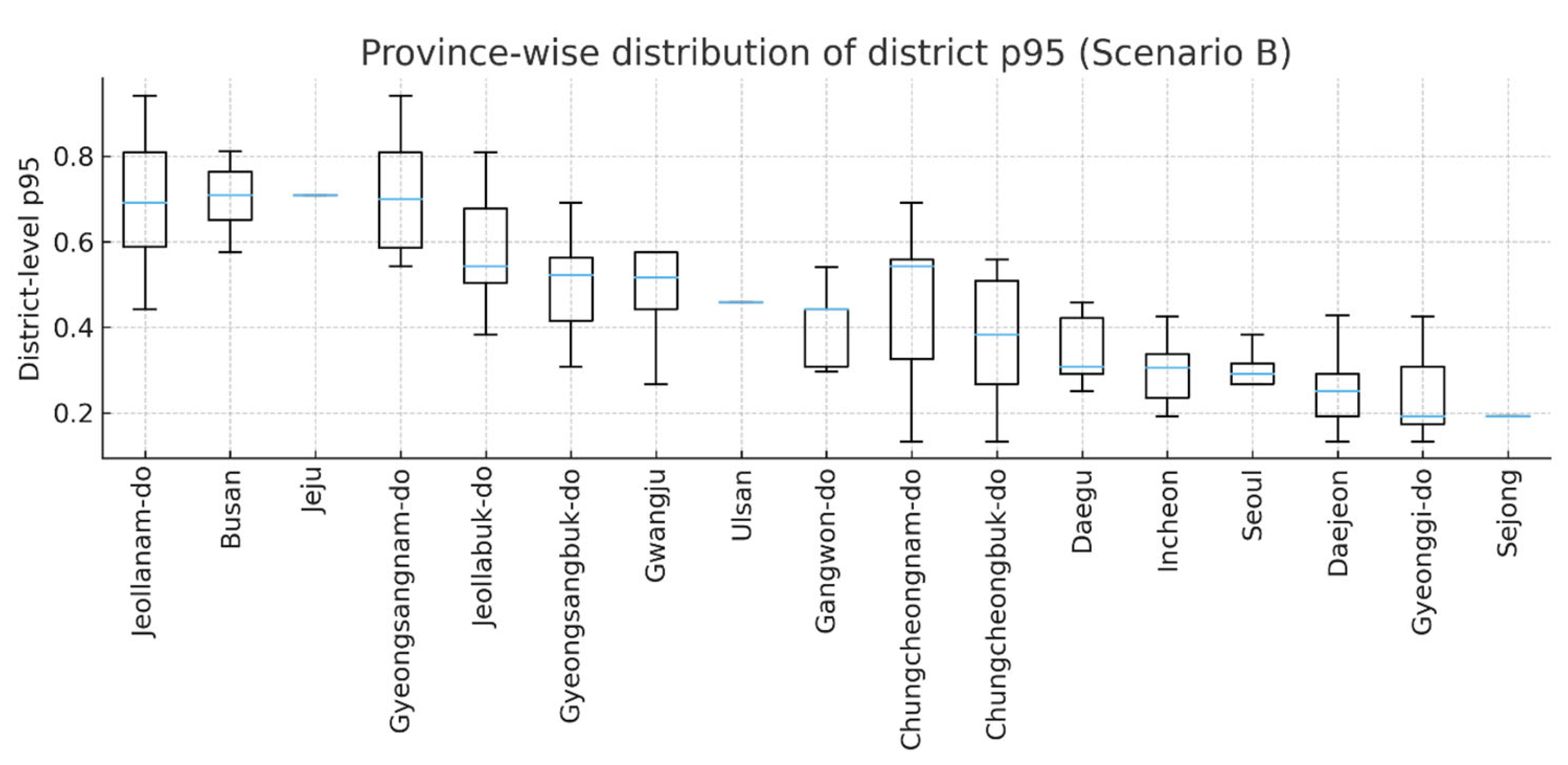
Beyond spatial autocorrelation (Moran’s I/LISA), we quantify spatial inequality of risk across provinces. Province-wise boxplots of the district-level p95 (Scenario B) reveal clear spatial inequality across regions. The interquartile range (IQR) of p95 differs markedly between provinces, indicating that some provinces contain districts with much wider spreads of risk, whereas others display comparatively compact distributions: provinces such as Gyeonggi-do, Daejeon, and Chungcheongbuk-do exhibit wide spreads (high IQR/CV), whereas Busan and Jeju show tighter distributions (low IQR/CV). Median levels also vary by province, pointing to systematic between-province differences in risk (Figure 14; see Table 20).
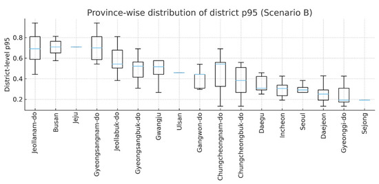
Figure 14.
Province-wise distribution of district-level p95 (Scenario B). Boxplots summarize p95 across districts within each province (ordered by provincial mean). The central line denotes the median; boxes span the interquartile range (Q1–Q3); whiskers extend to 1.5 × IQR; outliers are suppressed for readability. Computed from districts with ≥1 protected tree under Scenario B weighting (wH = 0.35, wR = 0.40, wS = 0.25). These province-wise boxplots (Scenario B) also indicate pronounced between-province inequality and within-province heterogeneity of district-level p95. The blue line for Jeju indicates the p95 value of a single district (no box is shown).

Table 20.
Province-level dispersion highlights (district p95, Scenario B). Top and bottom provinces by district-level p95 dispersion (CV). Values are computed under Scenario B; ordered within each group by CV. Interpret Jeju (n = 2) with caution due to small sample size.
Provinces in the high-dispersion group (top-quartile CV; e.g., Gyeonggi-do, Daejeon, Chungcheongbuk-do) contain districts that differ widely in risk, implying the need for sub-provincial targeting of inspections and adaptation measures. By contrast, low-dispersion provinces (bottom-quartile CV; e.g., Busan, Jeollanam-do) show comparatively compact distributions, for which province-wide programs may be more efficient (Figure 14; Table 20).
3.6. Robustness Checks for Weighting and Normalization Schemes
3.6.1. Scenario Sensitivity (Based on District-Level Mean Risk)
As noted earlier in Section 3.2.4, a preliminary sensitivity check was conducted by examining the Top 20 high-risk counties across scenarios. Here, the scenario sensitivity test is extended through a more rigorous statistical procedure, namely Spearman’s rank correlation analysis of district-level mean risk across scenarios.
The results confirm robustness: Spearman’s ρ was 0.9826 between Scenarios A and B, 0.9985 between Scenarios A and C, and 0.9764 between Scenarios B and C (all p ≤ 0.05), as shown in Table 21. These values demonstrate that the rankings are largely insensitive to scenario choice.

Table 21.
Scenario-based sensitivity (Spearman ρ). Scenario-based sensitivity checks indicate that district rankings are highly stable across weighting schemes (Spearman’s ρ: A–B = 0.983, A–C = 0.999, B–C = 0.976; all p < 0.001). These results suggest that our substantive conclusions are robust to reasonable changes in the relative weights of heat, precipitation, and species sensitivity.
However, as shown in Table 22, a few counties (e.g., Gunsan and Dong-gu, Daegu) exhibited relatively large shifts in rank depending on scenario, and these may reasonably be classified as boundary cases.

Table 22.
Top 20 counties with the largest rank fluctuations across scenarios.
It should also be noted that because the scenarios differ only in weighting schemes, the scenario sensitivity test simultaneously serves as a robustness test against changes in weight composition.
3.6.2. Normalization Schemes
When the normalization method was changed from [0–1] linear normalization to z-standardization (applied to H, R, and S alike), the district-level rankings of mean risk remained nearly identical (Spearman’s ρ = 0.995, p < 10−220, n = 234). In other words, the ordering of mean risks was preserved almost perfectly across normalization methods.
At the same time, Top-K Jaccard analysis revealed a more nuanced picture. For the Top 10, the Jaccard index was only 11.1% (with just 2 counties overlapping). For the Top 20, overlap rose to 48.1% (13 counties in common, about half). For the Top 30, the overlap increased to 71.4% (25 counties in common, a substantial degree of stability). By the Top 50, the rankings under the two normalization methods were completely identical (J = 1.00).
This demonstrates that while overlap increases with K, making the rankings considerably robust from the Top 30 onward, the very uppermost tier (Top 10) remains relatively sensitive. Therefore, for purposes of policy prioritization, it is most appropriate to base decisions on the intersection of the Top 20–30, where results are both stable and substantively meaningful.
3.7. Boundary Visualization and Interpretation
Using the same district-level p95 (Scenario B), the fuzzy boundary view (x: p95; y: probability of priority status μ, B = 1000) shows that the bulk of high-p95 districts cluster at μ ≈ 1, indicating robust priority under the national rule. By contrast, a small near-threshold set (n = 4) lies very close to the empirical cutoff and exhibits μ ≈ 0.5 together with wider p95 confidence intervals, signaling threshold sensitivity. These cases are most appropriate for province-specific screening or contextual judgment, while the remainder are stably prioritized. The empirical national 90th-percentile cutoff was p95 ≥ 0.6917 (ties included). See Figure 15 for the scatter and Table 23 for the near-threshold set.
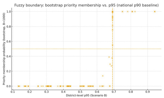
Figure 15.
Fuzzy boundary for national 90th percentile on district-level p95 (Scenario B; B = 1000). Scatter of districts (x: p95; y: probability of priority status μ, i.e., the fraction of bootstrap replicates in which the district is classified as priority). The vertical dashed line marks the empirical national 90th-percentile cutoff (p95 = 0.6917); the horizontal dotted line marks μ = 0.5. Points near the intersection denote threshold-sensitive districts likely to flip under small perturbations; upper-right points indicate robust priority (μ ≈ 1). Values are computed from per-tree risk (Scenario B); ties at the threshold are included.

Table 23.
Threshold-sensitive (near-threshold) districts under the national 90th-percentile rule (Scenario B; B = 1000). Districts identified by either criterion—within ±2 percentiles of the national 90th-percentile cutoff or with μ ∈ [0.4,0.6]. Columns: n (trees), p95, 95% CI, Priority status (national 90th-percentile rule) [0/1], Probability of priority status (μ, bootstrap B = 1000), and Percentile rank of p95 in the national distribution. This shortlist is intended for targeted review of threshold-sensitive cases.
Making the decision boundary explicit improves transparency and operational use. For robust districts (μ ≈ 1), the national 90th-percentile priority is stable, so action can proceed with confidence. For threshold-sensitive districts (μ ≈ 0.5), local authorities and inspection teams may (i) consult province-specific 90th percentile as a secondary screen, (ii) incorporate site context (e.g., drainage, staffing/management capacity), or (iii), where resources allow, seek targeted stakeholder input specifically for this small near-threshold set.
4. Discussion
4.1. On the Interaction Between Species Distribution and Regional Vulnerabilities—In Relation to RQ1
The nationwide distribution of protected trees and the region-specific climatic vulnerabilities presented in this study clearly demonstrate that risk landscapes emerge at the intersection of species’ physiological thresholds and regional climate regimes. The continuous high-risk belt observed along the southern and southwestern coasts corresponds closely to patterns of heatwave frequency and localized heavy rainfall. Even within this same macro-region, however, variations in species composition and micro-environmental conditions (e.g., soil aeration and drainage, degree of paving, and urban heat island effects) result in substantially different levels of experienced risk. Ultimately, vulnerability can only be adequately explained when the three levels—individual, species, and region—are considered in combination. Section 4.1’s descriptive statistics and distributional overview provide a consolidated framework for capturing this multilayered structure.
4.2. On the Construction of the Composite Risk Index and Scale-Level Differences—In Relation to RQ2
The composite risk index, computed at the level of individual trees by combining heat and rainfall exposures with species sensitivities, was aggregated to provincial and district scales, where both means and tails (e.g., 90th percentile, p95) were analyzed. The preservation of rank order during normalization and the absence of excessive distortion in the upper-tail mass (Figure 2, Figure 3 and Figure 4; Table 4) ensure fairness in relative comparisons across national, provincial, and district scales. Consequently, counties with disproportionately thick tails—despite having similar mean values—emerge as more vulnerable to extreme events, offering signals of priority that differ from those based on mean values alone. This highlights the study’s contribution in moving beyond the “mean-centered” convention toward a “tail-sensitive” decision-making paradigm.
4.3. On the Location, Typology, and Species Differences in High-Risk Counties—In Relation to RQ3
Counties with high composite risks cluster in specific regions, and these can be classified into heat-driven, rainfall-driven, species-sensitivity-driven, and composite types. Each type entails different priorities and prescriptions. For instance, rainfall-driven counties require immediate interventions in drainage, permeability, and soil depth; heat-driven counties prioritize shading, evaporative cooling, and soil moisture retention; while composite counties necessitate combined treatment packages addressing both. At the species level, clear differences in tolerance to heat and excess moisture indicate that even within the same region, management intensity must vary depending on the dominant tree species present.
4.4. On the Meaning of Spatial Patterns and Visualization—In Relation to RQ4
The spatial distribution of risk is not random scatter but a structured pattern. Global Moran’s I confirmed the presence of positive spatial autocorrelation, while LISA maps identified the specific locations of High–High hot spots and Low–Low cold spots (Figure 10 and Figure 11). By overlaying mean-risk bubbles with HH cluster boundaries, one can simultaneously interpret “where risk is high” and “whether those high values are spatially connected.” This joint view enables the identification of boundary and isolated zones—areas of higher management complexity—that cannot be captured by single global statistics alone. Moreover, the fact that cluster locations are reproduced with high similarity even when the neighbor definition (k) is varied indicates that the outlines of the core high-risk regions are not unduly dependent on analytical settings.
The mapped variable represents the district-level p95—the 95th percentile of per-tree risk—derived from heat exposure, precipitation exposure, and species sensitivity. Because p95 is explicitly climate-driven by design, positive global autocorrelation (Moran’s I) indicates that geographically adjacent districts experience similarly high climatic stress (e.g., warmer coastal belts or rainfall-intense corridors), rather than coincidental similarity in administrative rankings. Local indicators of spatial association (LISA) further refine this pattern: “high–high” clusters reveal regional pockets where both heat and precipitation pressures jointly elevate the upper tail, whereas “low–low” clusters correspond to areas of shared climatic mildness. Mixed zones (“high–low”/”low–high”) frequently occur at ecological or management boundaries and warrant on-the-ground validation. This ecological interpretation follows directly from the construction of p95 and its input variables. At finer spatial scales, land-use factors such as urban heat island intensity, canopy fraction, and impervious surface coverage may further modulate the signal. Although such layers are beyond the current national-scale scope, their integration represents a clear next step for future iterations.
4.5. On Robustness to Weighting and Normalization Changes—In Relation to RQ5
District-level risk rankings showed very high consistency across the three weighting scenarios (A/B/C), while shifts in normalization methods did not substantively alter the identification of extremes. This demonstrates that the interpretability of results is not undermined by design choices in indicator construction, thereby greatly enhancing predictability for policy applications. However, micro-ordering in intermediate ranges was somewhat sensitive to weighting changes, suggesting that policymakers should explicitly articulate “policy-weighting profiles” (e.g., prioritizing heat vs. rainfall vulnerability) and present results in parallel tables. From this follows a natural allocation principle: robust high-ranking regions are assigned to immediate intervention portfolios, while more volatile regions are targeted for enhanced monitoring and experimental interventions within an adaptive portfolio framework.
4.6. Confirming Priority Areas and Implementation Strategies—With Particular Emphasis on RQ6
Even with the current dataset, priority management areas can be identified by applying a rule that requires not only high mean values but also the actual presence of “high-risk individuals.” In this study, a district was defined as a priority area if, under the baseline Scenario B, it contained at least one tree exceeding the nationwide 90th-percentile threshold. This rule explicitly incorporates tail risks that may be obscured by averages. The criterion is straightforward, making field application practical, and is directly linked to the tabular and cartographic outputs that summarize the number and proportion of threshold-exceeding individuals, dominant sensitivity labels (heat/rain/composite), representative species, and recommended interventions (see Table 7, Table 8, Table 9 and Table 10).
The geographic core of priority areas emerges consistently. Counties in the southwestern and southeastern regions repeatedly rank high by both mean and tail criteria, and they reappear across scenarios, forming a robust top group. This set is suitable both as the starting point for short-term projects and as anchor sites for medium-term planning. In these priority zones, it is rational to rapidly deploy “combined packages” that integrate individual-level treatments with site-based infrastructure interventions. For rainfall-driven areas, key measures include drainage maintenance, conversion to permeable pavements, and installation of rain gardens and detention basins. For heat-driven areas, shading structures, canopy management, mulching, and fine mist sprinklers are central. Composite-type areas require simultaneous deployment of both sets. For species-sensitivity-driven zones, strategies should emphasize intensive care for heat- or flood-intolerant species, grafting and trial planting of substitute species, and microhabitat improvements that enhance long-term resilience.
Boundary and isolated zones require fine-tuning. Where LISA identifies Low–High clusters, tree-level risks may be amplified by spillovers from adjacent high-risk regions, making it necessary to preemptively reinforce soils, moisture, and shading while designing management routes that connect with the “core” zones. Conversely, in High–Low areas, localized bottlenecks—such as pest outbreaks, soil salinity, or root-space constraints—must first be diagnosed, followed by tailored interventions combining tree health recovery programs with improvements in physical site conditions. Because administrative boundaries do not always align with spatial-cluster boundaries, it is advisable to link layered visualizations such as Figure 13 directly to on-site inspection checklists.
Budget allocation can follow a staged design grounded in robustness. Counties that remain consistently high-ranked across scenarios and normalization methods should receive “execution-oriented” budgets, while those with volatile rankings should be allocated “monitoring- and experiment-oriented” budgets first. The former category directly feeds into short-term implementation lists, while the latter reduces uncertainty through additional measurements (e.g., surface temperature, soil moisture, irrigation volume) and pilot interventions. This dual allocation is grounded on two axes of evidence—Spearman rank correlations and LISA Jaccard similarities—thereby enhancing both the transparency and legitimacy of policy decision-making.
Finally, a notable strength of the priority selection rule lies in its “open structure.” As more data accumulate, the resolution can naturally be scaled up from district to township and plot levels, while integrating species-specific physiological thresholds and site-based indicators such as urban heat profiles and soil permeability coefficients. This will simultaneously improve the precision of candidate identification and the tailoring of prescriptions. Even at this stage, the tabulated outputs can be directly converted into “priority management cards” (containing fields such as district name, exceedance rate, dominant driver, representative species, recommended interventions, and responsible agency), enabling immediate operational use by local authorities.
In sum, the framework presented here enables the operation of a full “selection–implementation–evaluation” cycle under resource constraints. Robust high-ranking regions receive immediate intervention packages, volatile regions are assigned to observation and experimental portfolios, and boundary/isolated zones undergo fine-tuned adjustments. This tripartite strategy is grounded in the complementary signals provided by mean and tail metrics, spatial clusters, and robustness checks. Rather than eliminating uncertainty, such a structure progressively narrows it into manageable categories, serving as a platform for adaptive policy experimentation.
Building upon this selection–implementation–evaluation framework, the next essential step is to establish a systematic monitoring system that can provide standardized, longitudinal evidence for model validation and policy feedback.
4.7. Building a National Monitoring Framework: International Alignment and Practical Pathways
While standardized time-series data on protected-tree health are not yet available at the national level, establishing such a system has become an urgent next step for policy and research, as it would enable longitudinal verification of the model’s risk index and strengthen its empirical rationality.
Many countries already register and protect monumental or heritage trees within established legal and administrative programs. Italy maintains a national register of monumental trees under Law 10/2013 and the 2014 Ministerial Decree, with periodic updates and publicly available datasets [22]. Japan combines Natural Monuments under the Cultural Properties Protection Law with a protected-tree system administered across national, prefectural, and municipal levels, and utilizes regular national forest inventories (NFI) to update management plans [23,24,25]. Greece—especially in relation to ancient olive trees—emphasizes standardized dossiers and local or academic documentation [26].
Building upon these systems, our study introduces a district-level risk layer derived from individual-tree data: for each district, the 95th percentile of per-tree risk highlights the upper tail of climate stress. This quantitative layer does not replace existing legal or cultural criteria; rather, it complements them by identifying where current climatic risk is comparatively higher, thereby supporting inspection plans and resource allocation with transparent evidence.
At the practical level, the national distribution of district-level p95 values suggests a three-tier management framework. Districts in the top 10 percent nationally (≥90th percentile) may be designated as Priority zones, those in the upper 10–25 percent as Watchlist, and all others as Routine. These categories can guide inspection frequency and budget allocation: Priority districts require more frequent checks, Watchlist districts require periodic verification, and Routine districts require regular rounds. Where within-province variation is large (e.g., higher CV or IQR), inspection frequencies can be adjusted accordingly. This adaptive rule integrates smoothly with Japan’s periodic surveys and Italy’s registry updates, maintaining existing legal frameworks while enriching them with a climate-risk perspective.
A long-term monitoring scheme can begin modestly and remain cost-efficient. Routine inspections can collect a standardized, lightweight metadata set—condition class four to five levels, photograph, location tags, and brief incident notes—using a unified form. Periodic recomputation of p95 and related percentiles every one to two years would capture key trends without excessive data burden, while event-triggered updates can follow major climatic extremes. Every five years, a more comprehensive review could reassess model assumptions, data quality, and local linkages, similar to Japan’s NFI rhythm, establishing a balanced two-layer schedule of short-term updates and periodic strategic evaluation. Municipal dashboards and concise operating guidelines can further support implementation without the need for large IT investments, specifying inspection frequencies and emergency response procedures.
Such a framework allows phased, realistic national roll-out. Initial efforts could compute district-level p95 from existing data, formalize the three-tier rule, and test it in pilot provinces. Monitoring operational indicators—inspection workload, findings, and incident responses—would inform gradual scaling. As resources permit, five-year review cycles and richer dossier standards can be institutionalized.
Overall, this monitoring framework complements existing legal and cultural systems by adding a quantitative climate-risk dimension. It aligns with Italy’s MASAF registry, Japan’s protected-tree and NFI systems, and Greece’s dossier-based documentation, showing both international coherence and domestic feasibility within Korea’s current administrative and budgetary constraints.
5. Conclusions
5.1. Summary of Key Findings and Contributions
This study developed a composite risk index at the individual-tree level by combining climatic exposures (heat and rainfall) with species-specific sensitivities, and analyzed it across multiple scales—national, provincial, and district. In doing so, it not only provided rankings but also illuminated the patterns and underlying drivers of risk, while simultaneously pointing toward actionable directions for immediate management. The academic and policy contributions are significant, particularly in that this is a large-scale empirical analysis encompassing virtually the entire population of protected trees across South Korea, rather than being limited to selected case studies.
The conclusions are supported by the structural signals inherent in the data rather than by arbitrary assumptions, as supported by the preservation of rankings and tail distributions across normalization methods, the high consistency observed across different weighting scenarios, and the robust reproduction of spatial cluster structures regardless of analytical settings. This study used both mean and tail (upper quantile) indicators, along with LISA-based core–boundary classifications. These combined approaches reveal extreme and concurrent risks that mean-centered decision-making had previously overlooked. They also connect these risks directly to a cycle of selection, implementation, and evaluation that can be applied in practice.
Most notably, this study defined priority management areas not simply as those with high averages but as those where threshold-exceeding individuals actually exist. This rule is clear, straightforward to apply, and flexible enough to increase precision as new data are integrated. As a result, both short-term intervention targets and medium-term strategic hubs can be identified simultaneously. Information that integrates mean and tail signals with risk typologies—such as heat, rainfall, composite, and species sensitivity—provides practical guidance. It helps design site-based infrastructure measures, including drainage, permeable surfaces, water retention, and shading. At the same time, it informs tree-level interventions such as canopy and root management, pest control, substitute species trials, and grafting. In boundary and isolated zones, where administrative and spatial-cluster boundaries may not align, the framework prompts fine-tuned adjustments, while in volatile regions it recommends strengthened monitoring and pilot interventions to reduce uncertainty, thereby constituting an adaptive portfolio.
The methodological contributions are also clear. First, by implementing an individual-based index that captures concurrent extremes, the study highlighted the policy significance of risks masked by averages. Second, robustness checks for weighting and normalization were incorporated as integral parts of the interpretation process, clarifying the stability of extremes and the adjustability of intermediate regions. This separation of “normative choices” (what to prioritize) from “technical choices” (how to combine indicators fairly) enhances transparency and reproducibility in indicator use. Third, by combining spatial autocorrelation with cluster visualization, the study confirmed that risks are structured signals rather than random noise, thereby providing policy tools to design both regional-scale priorities and fine-grained boundary adjustments.
5.2. Limitations and Future Directions
Nevertheless, the study has clear limitations. First, the use of a nationwide single threshold (90th percentile) may not fully capture local differences in management capacity, microclimate, or land cover. Second, introducing regional or climate-zone-specific thresholds and integrating stakeholder preferences through multi-criteria decision analysis (MCDA) would be essential for enhancing fairness and acceptability in implementation, but this was not undertaken here. Third, the species sensitivity labels remain at the prototype stage. They are based on literature and data base expressed in categorical terms; however, if extended in the future to incorporate continuous physiological and growth indicators (e.g., tree vigor, water stress, pest history) and site-specific environmental metrics (e.g., surface temperature, soil permeability and aeration, proportion of paved or shaded area), the precision of risk estimation would be substantially improved. To strengthen the current three-point proxy (0.3/0.6/0.9) without launching a large-scale data program, we plan two low-cost measures in the near term. (i) A focused expert calibration will be conducted for the top 10–15 species in Priority districts using a concise one-page rubric, allowing minor score adjustments (±0.1) where justified. (ii) Routine inspections in Priority districts will include lightweight field metadata—condition class (four to five levels), photograph, and geotag—to build a small but consistent longitudinal dataset for proxy calibration. As resources permit, this framework will be expanded to incorporate trait- or physiology-based metrics and richer site covariates. Fourth, strengthened data integration—combining field inspections, remote sensing, and citizen science—together with longitudinal monitoring will be required to iteratively adjust boundaries and to trace the cumulative effects of climate trajectories, urbanization, and management interventions.
Despite these limitations, the policy implications are clear. Robust high-risk regions should receive immediate execution-oriented packages; regions with volatile rankings should be allocated observation- and experiment-oriented budgets; and boundary or isolated zones should be prioritized for fine-tuned strategies. To support this, coordination across central, provincial, and local levels should establish (1) standardized on-site checklists (region × factor × species × recommended measure), (2) a regular data management system (updated 1–2 times per year, with open-access mapping services), and (3) ex-post evaluation metrics (e.g., reduction in exceedance rates, recovery of tree vigor, avoidance of damage during extreme events). Particularly, the rule of “presence of threshold-exceeding individuals” is an immediately applicable operational criterion, and its resolution can be gradually scaled up (district → township → plot) and refined as data accumulate.
In sum, this study considered multiple signals simultaneously—means and tails, clusters and boundaries, robustness and volatility—and translated them into differentiated strategies of execution, observation, and fine-tuning. This framework provides a pathway for maximizing tangible risk reduction effects even under resource constraints. Future research that integrates localized thresholds, continuous physiological data, high-resolution environmental indicators, and long-term time series will help advance the conservation of protected trees from short-term projects toward becoming a sustainable component of public infrastructure.
Author Contributions
Conceptualization, S.K.; methodology, S.K.; software, S.K.; validation, S.K.; formal analysis, S.K.; investigation, S.K.; resources, S.K.; data curation, S.K.; writing—original draft preparation, S.K.; writing—review and editing, S.K.; visualization, S.K.; supervision, Y.N.; project administration, Y.N.; funding acquisition, Y.N. All authors have read and agreed to the published version of the manuscript.
Funding
This research was supported by the Ministry of Education of the Republic of Korea and the National Research Foundation of Korea (NRF), grant number NRF-2023S1A5C2A02095114. The APC was funded by the Ministry of Education of the Republic of Korea and the National Research Foundation of Korea (NRF).
Institutional Review Board Statement
Not applicable.
Informed Consent Statement
Not applicable.
Data Availability Statement
The original contributions presented in this study are included in the article. Further inquiries can be directed to the corresponding author.
Conflicts of Interest
The authors declare no conflicts of interest.
References
- Kozlowski, G.; Song, Y.G. Importance, Tools, and Challenges of Protecting Trees. Sustainability 2022, 14, 13107. [Google Scholar] [CrossRef]
- Seo, J.Y.; Lee, Y.Y.; Lee, J.K. A Study on the Improvement of Environment through the Analysis of Rearing Status of Law-Protected Trees—With Focus on Law-Protected Trees in Hwasung City. J. Korean Inst. Tradit. Landsc. Archit. 2009, 27, 93–102. Available online: https://www.kci.go.kr/kciportal/ci/sereArticleSearch/ciSereArtiView.kci?sereArticleSearchBean.artiId=ART001427646 (accessed on 20 October 2025).
- Kim, K.H. Analysis of Current Status and Utilization of Protected Trees in Gyeongsan City. J. Agric. Life Sci. 2011, 45, 69–83. Available online: https://www.kci.go.kr/kciportal/ci/sereArticleSearch/ciSereArtiView.kci?sereArticleSearchBean.artiId=ART001550106 (accessed on 20 October 2025).
- Yoon, Y.H.; Ju, J.H. Assessment of Growth Conditions and Maintenance of Law-Protected Trees in Je-Cheon City. J. Korean Inst. Tradit. Landsc. Archit. 2010, 28, 67–74. Available online: https://www.kci.go.kr/kciportal/ci/sereArticleSearch/ciSereArtiView.kci?sereArticleSearchBean.artiId=ART001463281 (accessed on 20 October 2025).
- Heo, S.H.; Ha, J.H. A Study on Growth Conditions of the Protected Trees in Gyeongju-si. J. Environ. Sci. Int. 2004, 13, 883–890. Available online: https://www.kci.go.kr/kciportal/ci/sereArticleSearch/ciSereArtiView.kci?sereArticleSearchBean.artiId=ART000937590 (accessed on 20 October 2025). [CrossRef]
- Doo, C.E.; Lee, J.B.; Lee, J.K. A Study on Growth Condition and Management of Protected Trees in Kimpo. J. Korean Inst. Tradit. Landsc. Archit. 2012, 30, 125–134. Available online: https://www.kci.go.kr/kciportal/ci/sereArticleSearch/ciSereArtiView.kci?sereArticleSearchBean.artiId=ART001649537 (accessed on 20 October 2025).
- Kim, H.R.; Kim, D.Y.; Park, J.S.; Lee, K.E.; Park, W.J. A Study on Current Status and Management of Protected Trees in Gangwon-Province. J. Korean Inst. Tradit. Landsc. Archit. 2010, 28, 12–26. Available online: https://www.kci.go.kr/kciportal/ci/sereArticleSearch/ciSereArtiView.kci?sereArticleSearchBean.artiId=ART001437257 (accessed on 20 October 2025).
- Lee, S.H.; Ko, D.S. Protective Tree Management Technique Using LiDAR 3D Scan Data. J. Korean Inst. Inf. Technol. 2020, 18, 99–106. [Google Scholar] [CrossRef]
- Lee, S.O.; Lee, J.Y.; Kim, C.S. A Study on the Investigation and Evaluation Standards for the Management of a Protected Tree. J. Korean Inst. Tradit. Landsc. Archit. 2024, 42, 55–66. [Google Scholar] [CrossRef]
- Schmied, A.; Pillmann, W. Tree Protection Legislation in European Cities. Urban For. Urban Green. 2003, 2, 115–124. [Google Scholar] [CrossRef]
- Wyse, S.V.; Beggs, J.R.; Burns, B.R.; Stanley, M.C. Protecting Trees at an Individual Level Provides Insufficient Safeguard for Urban Forests. Landsc. Urban Plan. 2015, 141, 112–122. [Google Scholar] [CrossRef]
- Caiche, D.T.; Peres, R.B.; Schenk, L.B.M. Protected Trees: The Experience of the City of São Carlos/SP. Rev. Gest. Ambient. Sust. 2022, 11, e22995. [Google Scholar] [CrossRef]
- Ministry of the Interior and Safety. LOCAL DATA. Available online: https://www.localdata.go.kr/lif/lifeCtacDataView.do (accessed on 19 October 2025).
- Statistics Korea. Climate Change and Disaster Vulnerability. 2023. Available online: https://kostat.go.kr/boardDownload.es?bid=12311&list_no=428842&seq=3 (accessed on 19 October 2025).
- USDA Forest Service. Silvics of North America Vol. 1. Conifers (Agriculture Handbook 654). Washington, DC, USA. 1990. Available online: https://www.srs.fs.usda.gov/pubs/misc/ag_654_vol1.pdf (accessed on 19 October 2025).
- USDA Forest Service. Silvics of North America Vol. 2. Hardwoods (Agriculture Handbook 654). Washington, DC, USA. 1990. Available online: https://www.srs.fs.usda.gov/pubs/misc/ag_654_vol2.pdf (accessed on 19 October 2025).
- Plants For A Future. PFAF Plant Database. Available online: https://pfaf.org/ (accessed on 19 October 2025).
- National Institute of Biological Resources. Species Portal. Available online: https://species.nibr.go.kr/ (accessed on 19 October 2025).
- PictureThis. Online Plant Encyclopedia. Available online: https://www.picturethisai.com/wiki/plants (accessed on 19 October 2025).
- USDA Natural Resources Conservation Service. PLANTS Database. Available online: https://plants.usda.gov/ (accessed on 19 October 2025).
- CABI. CABI Compendium: Forestry. Available online: https://www.cabidigitallibrary.org/product/QF (accessed on 19 October 2025).
- Ministero dell’Agricoltura, della Sovranità alimentare e delle Foreste (MASAF). Elenco degli alberi monumentali d’Italia ai sensi della Legge n. 10/2013 e del Decreto 23 ottobre 2014. 2025. Available online: https://www.masaf.gov.it/flex/cm/pages/ServeBLOB.php/L/IT/IDPagina/11260 (accessed on 20 October 2025).
- Forestry Agency (Japan). State of Japan’s Forests and Forest Management—3rd Country Report of Japan to the Montréal Process; Forestry Agency, Government of Japan: Tokyo, Japan, 2019; Available online: https://www.maff.go.jp/e/policies/forestry/attach/pdf/index-8.pdf (accessed on 20 October 2025).
- Ministry of the Environment (Japan). Protected Areas in Japan; Government of Japan: Tokyo, Japan, 1995; Available online: https://www.env.go.jp/earth/coop/coop/document/ttmnc_e/08-ttmnce-4.pdf (accessed on 20 October 2025).
- Yasuhara, K.; Nakasizuka, T.; Nagae, Y.; Kumagai, Y. A Study on Forest Protection Management in Forest Reserve and Its Changes. J. Jpn. Inst. Landsc. Archit. 1992, 56, 187–192. [Google Scholar] [CrossRef][Green Version]
- Koniditsiotis, S. Registration and promotion of monumental olive trees in Greece. Adv. Soc. Sci. Res. J. 2020, 7, 107–121. [Google Scholar] [CrossRef]
Disclaimer/Publisher’s Note: The statements, opinions and data contained in all publications are solely those of the individual author(s) and contributor(s) and not of MDPI and/or the editor(s). MDPI and/or the editor(s) disclaim responsibility for any injury to people or property resulting from any ideas, methods, instructions or products referred to in the content. |
© 2025 by the authors. Licensee MDPI, Basel, Switzerland. This article is an open access article distributed under the terms and conditions of the Creative Commons Attribution (CC BY) license (https://creativecommons.org/licenses/by/4.0/).


