Using Dimensionality Reduction Methods to Explore the Social, Cultural and Geographical Reasons Behind Food Waste in the European Union

Abstract

The paper investigates disparities in food waste generation across European Union countries between 2020 and 2022, focusing on spatial and sustainability dimensions. It utilizes data for six key food waste parameters and a broad range of environmental, social and economic indicators. A combination of statistical methods, including correlation analysis, cluster analysis and Principal Component Analysis, uncovers multivariate patterns and identifies groups of countries with similar food waste characteristics and related factors. The paper highlights the temporal and spatial dynamics of food waste over the three-year period, particularly in light of the COVID-19 pandemic. While the total volume of food waste remained relatively stable across the EU, notable shifts occurred in waste sources. Household food waste peaked in 2021, likely due to increased time spent at home during pandemic-related lockdowns. Conversely, waste from retail, restaurants and food service sectors showed a consistent increase. The paper identifies non-trivial correlations between food waste and socio-economic variables, suggesting that differences in food waste generation across EU countries are influenced by a complex interplay of factors, including policy effectiveness, cultural practices, consumer behaviour and economic conditions. This comprehensive analysis of food waste patterns across EU countries and over time offers valuable insights for policymakers aiming to reduce waste and promote sustainability.

1. Introduction

The onset of the COVID-19 pandemic in early 2020 triggered unforeseen disruptions in global food systems [1,2]. Initial lockdowns led to rapid shifts in food availability, characterized by empty shelves in certain regions and significant surpluses of unsold produce in others [3,4]. This public health crisis quickly tested the resilience of the entire food supply chain [5]. Our recent food waste studies that utilized correlation analysis and cluster analysis [6], as well as Principal Component Analysis and one- and multidimensional linear regression [7], reveal a contrasting dynamic, in which the pandemic not only exposed systemic vulnerabilities but also prompted rapid adaptation and innovative responses, while reflecting and reinforcing existing patterns of socio-economic disparity.

The relationship between the COVID-19 pandemic and food waste proved to be multifaceted [8]. Specifically, supply chains experienced interruptions, consumer behaviours changed rapidly, and established patterns of production, distribution and consumption were disrupted [9,10]. Initial global reports indicated widespread disturbances, with farms facing challenges in delivering products to markets, processors encountering obstacles and retailers struggling to adapt to fluctuating demand [3,11,12]. Consequently, food that decays quickly, such as dairy, fruits and vegetables, was especially vulnerable. In fact, prior studies have indicated that some producers were compelled to dispose of substantial amounts of produce that could not be stored or redirected [13,14,15].

In contrast to the consistency observed in food waste patterns at earlier stages of the supply chain, household behaviours exhibited greater variability [16,17]. Initially, responses to the crisis involved widespread stockpiling, motivated by uncertainty rather than scarcity, leading to increased expiration of unused food [18,19]. However, as the pandemic progressed, a shift towards more careful meal planning and home cooking was observed, coupled with a decreased reliance on dining out [20,21]. Simultaneously, the closure of hospitality and institutional food service sectors resulted in substantial stock losses. To mitigate these losses [22], food donation networks and community-based programs expanded their operations, redirecting surplus food to vulnerable populations [23]. Food waste generation is influenced not only by proximal disruptions but also by deeper social, cultural and geographical determinants. For example, differences in diet, family size and composition, and urban versus rural residential contexts have been shown to influence the quantity and quality of waste.

Our ongoing work takes these observations further, exploring how crises like COVID-19 shape not only waste patterns but also the resilience and adaptability of food systems. Early results suggest that pandemic-era waste patterns reflected pre-existing socio-economic differences as much as they did the virus’s direct impact. This paper seeks to address existing research gaps by analysing how varied policy frameworks and cultural practices across European Union member states interact with food supply chains, thereby influencing food waste outcomes. Furthermore, it employs advanced dimensionality reduction techniques to uncover latent data structures, overcoming the limitations of previous studies that often lacked multivariate statistical approaches for disentangling complex interactions. The paper uses a comprehensive approach to explore the relationships between structural vulnerabilities, community-level coping mechanisms and socio-economic inequalities, which collectively shape both the intensity of disruptions and the rate of recovery. Initial results indicate that waste trends identified during the pandemic were not exclusively a direct consequence of the virus; instead, they mirrored and, in certain instances, intensified pre-existing disparities grounded in the social, cultural and economic frameworks of individual countries.

Against this backdrop, the paper analyses food waste trends in the European Union; by using six key indicators and applying dimensionality reduction methods, it explores how national trajectories cluster or diverge, and how social, cultural and geographical factors may have shaped these patterns. To better understand these patterns, this study focuses exclusively on EU member states, as coherent and comparable datasets for other regions are not available; this limitation is acknowledged as an important constraint of the research. Two guiding hypotheses inform our approach:

–

H-1: Variations in food waste generation across EU member states can be linked to underlying social, cultural and geographical characteristics, which influence both the scale and type of waste produced.

–

H-2: Changes in consumer behaviour, supply chain dynamics and institutional practices during the study period reflect deeper structural drivers that predate the pandemic but were brought into sharper focus by it.

By identifying these relationships, this research aims to contribute actionable insights for designing targeted waste reduction strategies, strengthening resilience and fostering sustainable food systems that are better equipped to withstand future crises. The paper underscores the innovative approach of distinguishing system-level factors from individual behaviours using Principal Component Analysis, thereby enabling policymakers to devise more effective interventions and tackle the underlying causes of food waste rather than merely its manifestations.

2. Literature Review

2.1. Food Waste: Definition, Origin and Effect

The EU Waste Framework Directive [24] provides a definition of food waste as all food, as defined in the General Food Law [25], which has become waste. Food is considered as a whole and applies throughout the entire food supply chain, from production through to consumption. Food includes inedible parts which are not separated from edible parts during production. According to this definition, it is not technically possible to completely eliminate food waste for several reasons: consumers cannot typically consume or reuse certain inedible parts (e.g., bones), some food must be discarded for safety reasons, and preventing food waste should not compromise food safety, or animal or human health. The EU’s definition of food waste excludes items that were not classified as “food” at the time of being discarded or removed from the supply chain (e.g., losses before harvest or slaughter) and does not encompass non-waste material such as surplus donated foods or by-products used for other purposes (e.g., animal feed). Food wastage occurs at every stage of the supply chain, including primary production; processing and manufacturing; retail and distribution; restaurants and food services; and households, both within homes and in out-of-home settings. Therefore, stages relating to residential properties/restaurants/services together constitute what is termed the “consumption” stage [26].

Food waste can be attributed to a number of causes, including losses in food production and processing, outdated quality standards, over-packaging, consumer perceptions and the influence of market trends [27]. In addition, food waste is often a consequence of consumer habits, convenience and economic considerations [28]. Overproduction and inefficient distribution systems, consumer attitudes and preferences [29], and lack of awareness and education about food waste can also play a significant role [29,30,31,32]. Furthermore, improper storage and handling, confusion over expiry dates (marked as “use by” or “best before” dates) and food labelling, as well as advertising and marketing strategies that encourage overconsumption, can also contribute to an increase in food waste. Lastly, cultural and social norms and aesthetic preferences for foods further compound this issue.

The effectiveness of food waste reduction initiatives is influenced by socio-cultural acceptance and public awareness, emphasizing the need for targeted communication strategies and policy instruments that consider local contexts.

2.2. Overview of EU Action for Preventing Food Waste

Preventing food waste became a specific political priority at the EU level in 2015, reflecting EU commitments made in the context of the 2030 Sustainable Development Agenda to reduce food waste by 50% and decrease food loss by the year 2030. The EU has implemented a specific strategy to decrease the amount of food that is lost or wasted that involves both regulatory and non-regulatory actions, first as part of the 2015 Circular Economy Action Plan and, more recently, under the 2020 Farm to Fork Strategy (a strategy that connects food production on farms directly to consumption by minimizing the distances food travels and the processes it undergoes between its origin in the fields and the final consumer). Since 2015, the Commission has been working on initiatives to clarify and harmonize relevant legislation. They have also supported the development and sharing of best practices and solutions to reduce food waste across the EU. Article 9 (Prevention of Waste) of 2018/851, amending Directive 2008/98/EC on waste, requires member states to implement measures aimed at decreasing food waste at all stages of the food supply chain [24]. It also promotes food donation and other forms of redistribution for human consumption, giving priority to human use over animal feed and the conversion of surplus food into non-food products [24]. Several guidelines, recommendations and informational publications have been published recently. While the European Union provides a standardized policy framework, its efficacy and practical application vary considerably among member nations. These disparities result in differing outcomes and highlight the significant impact of contextual factors on food waste dynamics.

The European Commission Directorate-General for Environment published guidelines on the preparation of food waste prevention programmes. This document is intended to serve as a valuable tool for waste management organizations, businesses, institutions, local authorities and environmental protection agencies. It covers the European policy framework concerning bio-waste, with a specific focus on food waste, and applies the waste hierarchy to food waste prevention and includes discussions on methods for measuring food waste, setting targets and implementing prevention strategies [33].

The EU Platform on Food Losses and Food Waste was established in 2016 to support all stakeholders in defining measures to prevent food waste, sharing best practices and evaluating progress made over time [34]. In 2019, the Commission adopted a common methodology for measuring food waste as a basis for monitoring food waste in the EU countries [35].

As part of the Circular Economy Action Plan, the European Commission has implemented EU 2017/C 361/01 Guidelines on food donations [36] to promote the efficient collection and distribution of safe and edible food to individuals facing food insecurity. This guidance clarifies provisions in EU legislation and helps remove barriers to food redistribution within the current EU regulatory framework. The main aspects involve following food safety and hygiene laws, keeping food at proper storage and transport temperatures, and permitting the donation of imperfect or expired foods.

The 2018/C 133/02 Guidelines for the feed use of food no longer intended for human consumption [37] address issues regarding feed utilization of food which is no longer intended for human consumption for commercial reasons or due to problems of manufacturing or certain defects, but which can be used in animal nutrition without compromising animal or public health. It helps prevent the nutrients in food from being composted, converted into biogas, or disposed of through incineration or landfill.

The recommendations for action in food waste prevention were compiled by the EU Platform on Food Losses and Food Waste to offer crucial guidance to all players in efforts to prevent food losses and waste, including EU citizens themselves [38]. The forward-looking recommendations include a set of horizontal or cross-cutting measures, as well as recommendations for action for primary production and food donation, for action at manufacturing, retail and consumer levels in hospitality/food services. The recommendations target both public and private entities, suggesting relevant actions for each group while emphasizing the need for cooperation among stakeholders. Despite existing EU guidelines, empirical research evaluating their effectiveness in reducing food waste remains scarce, underscoring the necessity for systematic assessment and standardized monitoring of member states’ results.

To guide effective actions, the authors of [39] present a framework for the evaluation of food waste prevention actions and explain its use in assessing the effectiveness and efficiency of such actions. To facilitate the continuous sharing of resources, latest developments and best practices, the Commission has set up a digital platform called the EU Food Loss and Waste Prevention Hub. This serves as a comprehensive resource for all stakeholders involved in food waste prevention [40].

Research and innovation aimed at tackling the prevention of food waste are supported by the European Commission, including the development of blueprints for the establishment of national public–private partnerships (e.g., Voluntary Agreements) to reduce food waste throughout the entire food supply chain [41]. The EU Research and Innovation Framework Programme Horizon 2020 and Horizon Europe are offering new opportunities for research and innovation to address food loss and waste [26].

3. Materials and Methods

3.1. Data

Our research is based on the datasets of the Statistical Office of the European Union published on the Eurostat website.

Table 1. Food waste absolute parameters.

Abbreviation	Indicators [kg/year/capita]
FP	Food waste from primary production of food—agriculture, fishing and aquaculture
MFP	Food waste from manufacture of food products and beverages
RDF	Food waste from retail and other distribution of food
RFS	Food waste from restaurants and food services
HHA	Food waste from total activities by households
TOTAL	Total food waste production, FP + MFP + RDF + RFS + HHA

contains the relevant tabular data about food waste datasets, while

Table 2. Structural indicators (types of indicators: environmental (EN), economic (EC), social (S) and geographical (G).

Abbreviation	Indicators	Unit	Type	Reference
AREA	Total area of the country	[km2]	G
CMR	Circular material use rate	[%]	EN	[42]
COFP	Consumption footprint index, year 2010 = 100	[dimensionless]	EN	[43]
ELET	Early leavers from education and training by sex	[%]	S	[44]
FECH	Final energy consumption in households per capita	[kg of oil equivalent]	EC	[45]
GDP_PC	GDP per capita value	[EUR/capita]	EC	[46]
GVAEGS	Gross value added in environmental goods and services sector, reference year 2010, chain-linked volumes at 2010 exchange rates	[EUR/capita]	EN	[47]
IAF	Inability to afford a meal with meat, chicken or fish (or vegetarian equivalent) every second day—EU-SILC survey	[%]	S	[48]
MF	Material footprint	[tonne/capita]	EN	[49]
MSDR	Severe material and social deprivation rate	[%]	S	[50]
MWG_PC	Municipal waste by waste management operations	[kg/capita]	EN	[51]
NSFT	Nights spent in tourist accommodation establishments by residents/non-residents	[number]	EC	[52]
POP	Population on 01.01.	[capita]	EC	[53]
POPDENS	Population density of the country (POP/AREA)	[capita/km2]	EC	[54]
PPGDP	Purchasing power adjusted GDP per capita, in purchasing power standards	[EUR/capita]	EC	[55]
PUKHW	Population unable to keep home adequately warm by poverty status	[%]	S	[56]
REG_BOR_PC	Border type area per capita	[km2/capita]	G	[57]
REG_COA_PC	Coastal type area per capita	[km2/capita]	G	[57]
REG_INT_PC	Intermediate type area per capita	[km2/capita]	G	[57]
REG_ISL_PC	Island type area per capita	[km2/capita]	G	[57]
REG_MOU_PC	Mountain type area per capita	[km2/capita]	G	[57]
REG_RUR_PC	Rural type area per capita	[km2/capita]	G	[57]
REG_URB_PC	Urban type area per capita	[km2/capita]	G	[57]
RMRPG	Relative median at-risk-of-poverty gap	[%]	S	[57]
RPS_PC	People at risk of poverty or social exclusion	[%]	S	[58]
TEA	Tertiary educational attainment by sex	[%]	S	[59]

summarizes the twenty-six selected structural indicators (environmental, social, economic and geographical parameters) that were collected for the EU-27 member states from 2020 to 2022. The downloaded data were directly used with no cleaning criteria. A rescaling to kg/year/capita units was applied before analysis. The total amount of food waste (TOTAL) is the sum of five distinct food waste parameters (Equation (1)): food waste from primary production of food (FP), manufacture of food products and beverages (MFP), retail and other distribution of food (RDF), restaurants and food services (RFS), and the total activity of households (HHA):

$$\mathrm{T}\mathrm{O}\mathrm{T}\mathrm{A}\mathrm{L}=\mathrm{F}\mathrm{P}+\mathrm{M}\mathrm{F}\mathrm{P}+\mathrm{R}\mathrm{D}\mathrm{F}+\mathrm{R}\mathrm{F}\mathrm{S}+\mathrm{H}\mathrm{H}\mathrm{A}$$

(1)

Relative food waste parameters were calculated by dividing the absolute parameters by the TOTAL value (FP_REL = FP/TOTAL, MFP_REL = MFP/TOTAL, etc.). Absolute parameters are quantified in kg/year/capita, indicating the annual per person amount in kilograms. Relative parameters represent the percentage distribution of the specific waste types at the country level.

3.2. Methods

The correlation and cluster analyses were performed by a self-developed Python language program that used Scikit-Learn and Scientific Python modules. PCA for the dataset was carried out using SciKit-Learn software (version 1.4.1).

3.2.1. Correlation Analysis

Linear (Pearson-type) and rank (Spearman-type) correlation tests were used to identify relationships between pairs of food waste parameters and structural indicators. The former are sensitive to approximately linear connection between the two variables, whereas the latter are capable of finding nonlinear but monotonic relationships. As the results did not reveal any non-trivial connections (see details in Section 4.1), Principal Component Analysis (PCA) and statistical tests for comparing clusters of countries were used to investigate the existence of multivariate and nonlinear connections.

3.2.2. Principal Component Analysis

The food waste dataset includes five independent variables for each country per year, theoretically allowing data points to be visualized in a five-dimensional space. To overcome this difficulty, Principal Component Analysis method was applied to reduce the number of dimensions of the dataset [60]. PCA initiates by calculating the average vector of the dataset and then determining the difference between each vector and the mean vector. The subsequent step involves identifying the direction in which the set of these difference vectors exhibits the greatest elongation—representing the “most important” direction—and describing it with a unit-length vector. Then, the subsequent (second, third, etc.) most important directions that are orthogonal to the previous ones are calculated.

In the case of food waste data, the original five dimensions were reduced to two dimensions using PCA, achieving a good approximation. Therefore, the principal component coefficients for each country and year were calculated and the temporal changes of the EU countries were visualized on a two-dimensional plot, with coordinates representing the PCA coefficients. This resulting plot was used to identify countries exhibiting similar behavioural patterns. In contrast to our prior similar PCA investigation [7], which was restricted to the year 2020 due to data limitations, the current research covers a three-year period from 2020 to 2022. All the three-year data (81 five-dimensional vectors) were used for a unique PCA-base vector calculation, and these were used to calculate the PCA components.

Given that the PCA method is based on linear operations, it was only applied to absolute food waste data, as absolute values in kg/capita/year units are additive, while relative components cannot be linearly combined.

3.2.3. Cluster Analysis

Cluster analysis is a multivariate statistical method used to find groups of similar items based on multidimensional numerical data. Our research applied this method to find subsets of EU members with comparable food waste characteristics. Clustering calculations were performed for the five-dimensional vectors of absolute (FP, MFP, RDF, RFS and HHA) and relative (FP_REL, MFP_REL, RDF_REL, RFS_REL and HHA_REL) food waste parameters. Linear scaling for the parameters was applied to obtain the same standard deviation in every coordinate. This standardization step was necessary because the average values for different parameters vary significantly. For example, household food waste (HHA) typically ranges from 50 to 100 kg/capita/year, while food waste generated during primary food production (FP) is commonly under 20 kg/capita/year. Therefore, a 10 kg/capita/year change in HHA represents a small change, while the same difference in FP is a dramatic alteration.

The K-means clustering method [61] was applied with N = 2–7 clusters. The elbow method was utilized to determine the optimal cluster number. According to the results, N = 5 appears to be the best choice. Qualitative analysis of various cluster numbers also confirmed that N = 5 represents the optimal selection. The classification of a country seemed forced when N was less than five; conversely, when N exceeded five, it led to an unwarranted fragmentation of clusters. The cluster members were listed and stacked histograms of absolute and relative food waste parameters were generated, where the EU members were grouped based on the clusters. Similar calculations were performed in our previous study [6], but then food waste data were only available for the year 2020. The present investigation expands the temporal scope to 3 years.

Following the identification of the groups of countries with similar food waste characteristics, structural indicators for each group were collected. The Mann and Whitney test (U test) was used to find statistically significant differences between these parameter-sets. Significant differences suggest a connection between the examined structural indicator and the food waste values. The advantage of this complex approach over the simple correlation analysis is two-fold. First, the comparison in this case is based on more data points, thereby minimizing the impact of uncorrelated measurement errors. Second, comparing only specific subsets of EU members can reveal connections that are not valid for the whole EU, while correlation analysis tries to find globally true connections.

4. Results and Discussion

4.1. Results of Correlation Analysis

Pearson- and Spearman-type correlation coefficients were calculated between all food waste parameters and the examined structural indicators. In all cases, the correlation coefficients did not exceed 0.7, leading to the conclusion that there is no simple dependence between such pairs. However, in some cases the coefficients were between 0.5 and 0.7, which indicates a possible connection, but this is not accepted as statistically well established. The absence of statistically significant results does not mean that there is no relationship between the amount of food waste and other parameters. It is possible that such a relationship only exists between certain groups of countries or that the correlation coefficient is reduced by a large measurement error for the parameters.

4.2. Results of Principal Component Analysis

Reducing the number of dimensions with PCA is a significant help in overviewing multidimensional data, but it inherently implies an approximation. The required level of precision should be determined by considering both the data’s accuracy and the research objectives.

Table 3. PCA reconstruction error in kg/year/capita units and relative explained variance values of percentages as a function of number of dimensions (D).

D	0	1	2	3	4	5
Accuracy	11.8	7.7	4.9	3.2	1.4	0.0
Rel. expl. var.		60.4	23.8	7.7	6.4	1.7

presents the average difference of the original components and the reconstructed values, depending on the number of dimensions retained. Naturally, increasing the number of dimensions results in smaller reconstruction error.

D = 2 was selected for analysis. This case has an accuracy of 4.9 kg/capita/year, falling within the expected range of measurement error. Relative explained variance values show that the third PCA component gives only a 7.7% improvement. While increasing to D = 3 offers a marginal reduction in average deviation, it complicates visualization. Since the numerical values provided by PCA are not used for further analysis in this article, but rather to review the nature of the changes, the accuracy provided by the two components is considered to be sufficient.

The results of the PCA algorithm contain the “mean vector” (m) and two “base vectors” (s1 and s2). All data points can be approximated as a linear combination of them, as is written in Equation (2).

$$foodwastevector\approx m+s_1\cdot P_1+s_2\cdot P_2$$

(2)

For each data point, the PCA coefficients, represented by the dimensionless quantities P₁ and P₂, are computed and used to characterize the food waste values for a specific country in a given year. This approach reduces the dimensionality of the data from the original five components (FP, MFP, RDF, RFS and HHA) to just two.

The numerical results are summarized in Equation (3). Figure 1 illustrates the graphical representation of the mean and base vectors.

$$\begin{gathered} FP\approx 13.2+0.148\cdot P_1+0.134\cdot P_2 \\ MFP\approx 30.2+0.970\cdot P_1-0.066\cdot P_2 \\ RDF\approx 11.6+0.186\cdot P_1+0.134\cdot P_2 \\ RFS\approx 15.1+0.043\cdot P_1+0.130\cdot P_2 \\ HHA\approx 69.4+0.014\cdot P_1+0.971\cdot P_2 \end{gathered}$$

(3)

Numeric values in equation (3) indicate that the first primary component (P₁) is mainly composed of food waste generated from manufacturing for food production (MFP), which carries the highest weight, followed by primary food production (FP) and the distribution of food production (RDF) components, which have smaller, but still considerable weights. These activities exhibit less dependence on individual behaviours and instead reflect the specificity of the economic sector (like agriculture, industry and transportation). Conversely, the P₂ component encompasses waste generated in households (HHA) as the most predominant factor; alongside restaurants and other food services (RFS) with a higher weight than in P₁, the other three components have smaller coefficients. Consequently, the second principal component is more heavily influenced by individual consumption, eating and cooking habits than the first one. It is worth noting that this separation of economic system-level parameters and individual behaviour parameters is an automatic result of PCA. This demonstrates that the method was capable of separating parameters that behave differently. According to these, a positive value for P₁ or P₂ means above-the-average economic system-level or individual food waste production, respectively.

Figure 2 illustrates the countries in the P₁-P₂ plane. Symmetrical logarithmic scaling was applied on the axes to show the extremely large values and to resolve the high-density part of the diagram near the origin on the same plot.

Each country is represented by a distinct colour and characterized by three data points of different sizes, corresponding to the years 2020 (small), 2021 (medium) and 2022 (large). These data points are interconnected by straight lines to allow for the observation of value trends across the specified period.

According to their P₁ and P₂ values, the countries can be divided into three groups:

• P₁ > 0: Belgium, Cyprus, Denmark, Greece, Ireland and the Netherlands. Their differences from the average food waste characteristics are mainly in the s1 direction, which means high excess in food waste from manufacture of food products (MFP) and significant excess in food waste from primary production (FP) and food waste from distribution of food production (RDF) components.
• P₁ < 0 and P₂ > 0: Austria, Germany, Italy, Latvia, Lithuania, Luxembourg, Malta, Portugal and Romania. They have below-average values for FP, MFP and RDF, but excessive values for food waste from households (HHA) and food waste from restaurants and other food services (RFS).
• P₁ < 0 and P₂ < 0: Bulgaria, Croatia, Czech Republic, Estonia, Finland, France, Hungary, Poland, Slovakia, Slovenia, Spain and Sweden. All of their food waste components are smaller than or equal to the average.

The examined period from 2020 to 2022 reveals two principal trends in the movement of individual countries within the P₁-P₂ plane. For a few countries, the differences across the three years are negligible (Croatia and Portugal) or marginal (Germany, Greece, Italy, Portugal, Slovenia and Slovakia). Conversely, half of the countries exhibit a notable shift from 2020 to 2021, but a much smaller shift from 2021 to 2022 (Austria, Belgium, Bulgaria, Cyprus, Czech Republic, Estonia, Latvia, Lithuania, Luxembourg, Malta, Poland, Romania, Spain and Sweden).

4.3. Results of Cluster Analysis

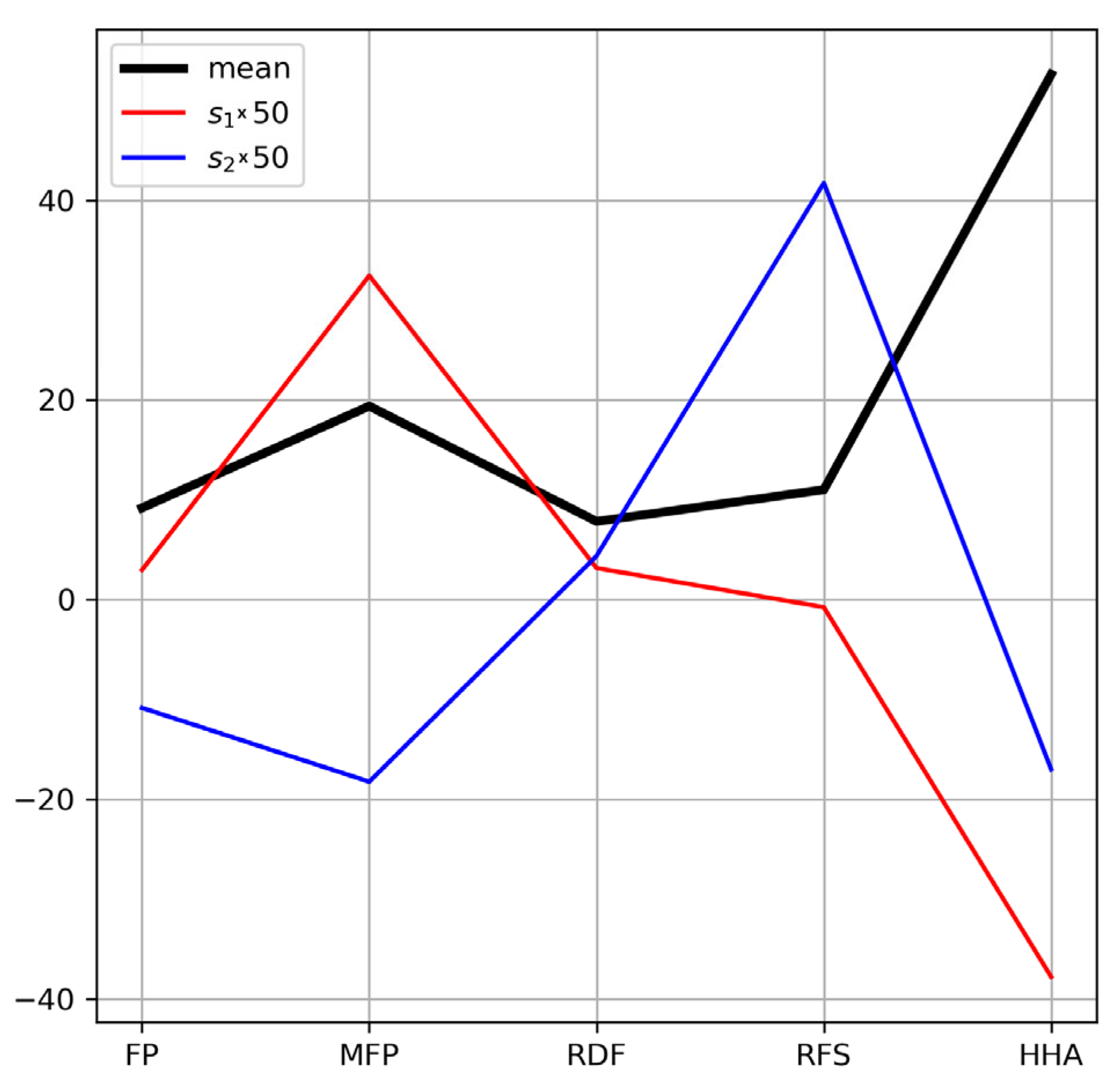
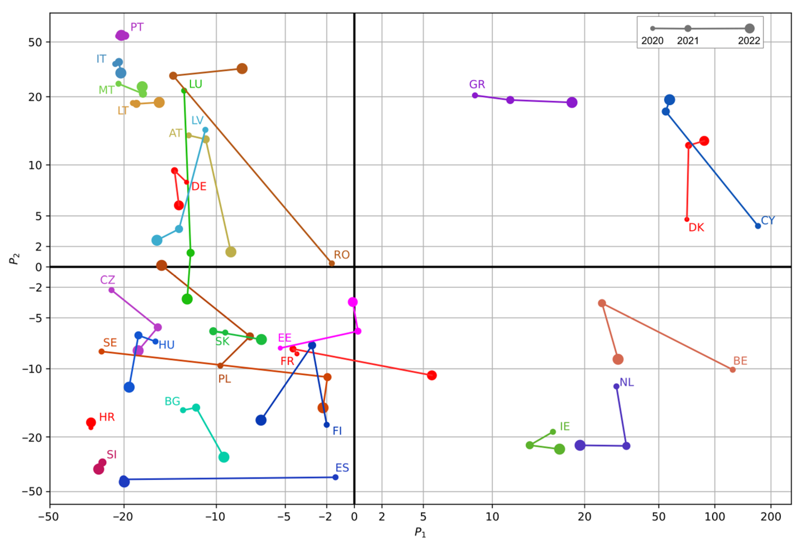
Absolute and relative food waste datasets contain five-dimensional vectors for the 27 EU members for the 3 years. One objective of our research was to detect patterns in these datasets. The widely used K-means clustering method was applied to find the groups of similar countries with standard scaling, i.e., applying a linear transformation on the data to obtain a standard deviation of 1 for each component. Without this normalization, changes in the components with the highest average values (HHA and MFP) would dominate the clustering and the effect of the other components would be negligible.

Calculations were performed for cluster sizes of N = 3, 4 and 5. Several similar patterns can be observed across these versions: Cyprus is typically isolated as a separate cluster and the former socialist states tended to group together. Investigating the results, we determined that N = 5 provided the most informative clustering. Therefore, the results for five groups are presented in this article.

The results of the K-means clustering calculations consist of N vectors: the so-called “cluster centres” and a labelling of each vector indicating its nearest cluster centres. This way the cluster centres represent the “typical” food waste parameter sets, while the cluster labels of the countries denote which cluster they most resemble.

4.3.1. Clusters of Absolute Food Waste Data

Clustering calculations were performed independently for each of the 81 food waste parameter vectors (27 countries for 3 years). Therefore, if the food waste profile of an EU member presents a significant shift during the 3-year period, data from different years for the same country may belong to different clusters.

The next list contains the members of the five clusters. When all three-year data for a specific country are grouped into the same cluster, only the two-letter abbreviation is displayed. Otherwise, the years are appended to the country code. Clusters are denoted by “ACL1”, “ACL2”, …, where “A” indicates that this clustering is based on the absolute food waste parameters. Figure 3 displays this clusterization on a color-coded map.

• ACL1 (1 member): CY.
• ACL2 (2 members): BE (2020) and DK.
• ACL3 (5 members): AT, DE, IE, MT and SI.
• ACL4 (7 members): GR, IT, LT, LU (2020), LV (2020), PT and RO (2021, 2022).
• ACL5 (16 members): BE (2021, 2022), BG, CZ, EE, ES, FI, FR, HR, HU, LU (2021, 2022), LV (2021, 2022), NL, PL, RO (2020), SE and SK.

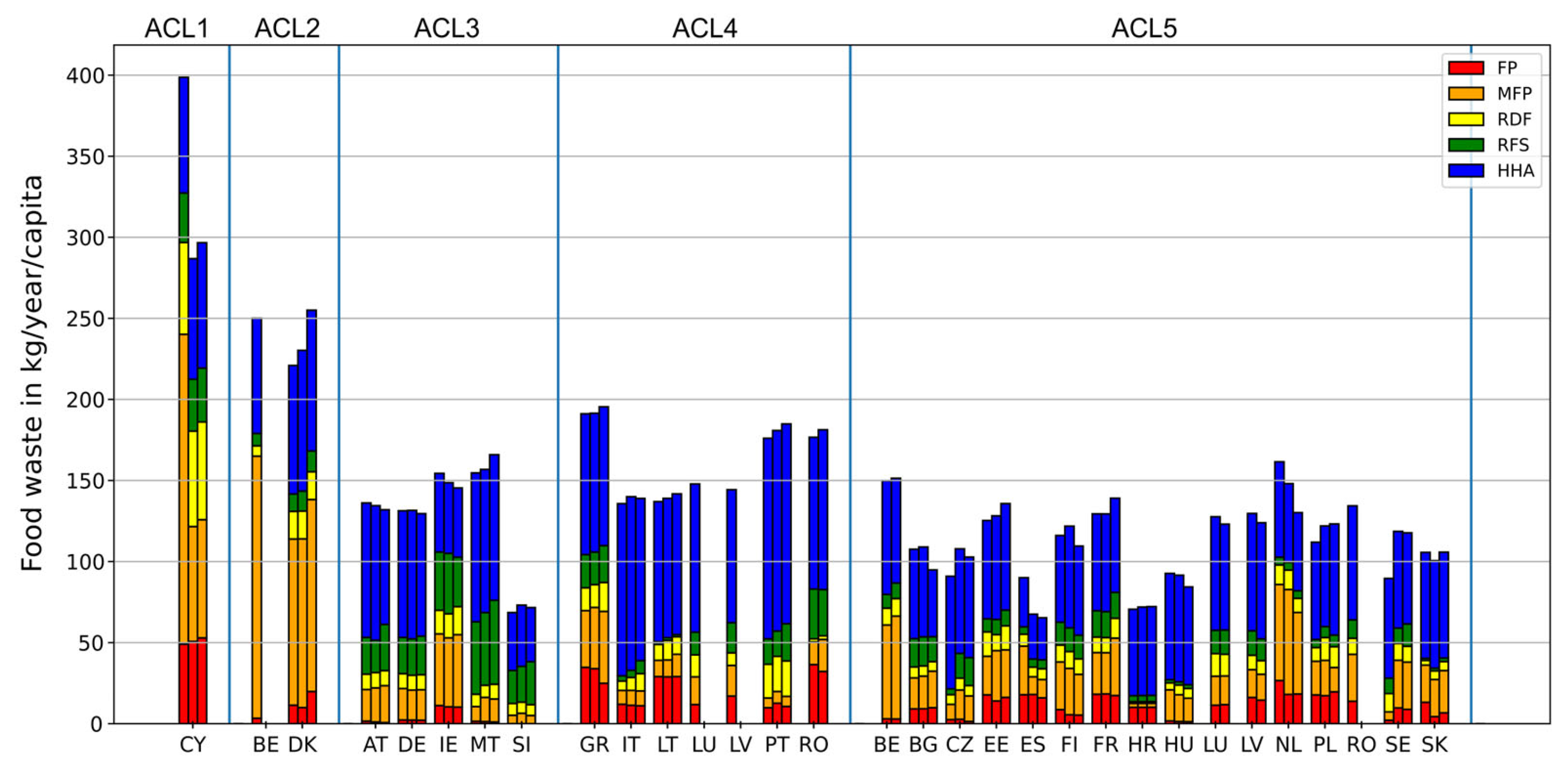
A graphical representation of this clustering is presented in Figure 4. The columns are sorted to reflect the results of the clusterization, and the blue vertical lines represent the barriers of clusters.

The analysis revealed that most countries preserved their respective cluster affiliations during the examined 3-year period. This indicates that the fundamental characteristics of these countries, as determined by the comprehensive and sectoral distribution of food waste, remained largely stable despite the COVID-19 pandemic. However, Belgium, Latvia, Luxembourg and Romania deviate from this pattern. In all these cases, the data from 2020 were grouped distinctly from the other two years. More specifically, the 2020 data for Luxembourg and Latvia are categorized in cluster ACL4, and for Belgium they are in ACL2, while their data from 2021 and 2022 are in ACL5. Conversely, Romania shifted from ACL5 in 2020 to ACL4 in 2021 and 2022.

Outlier data, such as those observed for Cyprus or Belgium in 2020, can be partly ascribed to methodological idiosyncrasies within specific reporting systems and highlight the need for increased harmonization in food waste data collection.

It is notable that the historical background aligns with the observed clustering patterns. For instance, almost all countries formerly belonging to the Eastern Bloc are in the ACL5 cluster (Figure 3 and Figure 4). The prevalence of the former Eastern Bloc nations in the same cluster indicates that previous consumption patterns and economic histories continue to affect present-day food wastage trends.

Table 4. Sectoral distribution of cluster centre values based on food waste per capita data in kg/capita/year units. Yellow background indicates the column-wise maximum.

	FP	MFP	RDF	RFS	HHA
ACL1	50.9	111.6	58.6	32.0	74.3
ACL2	11.1	121.6	14.4	10.9	81.0
ACL3	3.0	20.4	9.8	30.2	65.4
ACL4	21.6	16.7	12.1	14.4	97.9
ACL5	11.1	24.5	8.6	9.2	58.8

presents the cluster centre values, which serve as multivariate indicators representing the “typical” food waste characteristics of EU members. A yellow background highlights the maximum value in each column. In the line of ACL1, there are three of them, which indicates exceptionally large food waste production in three categories. On the other hand, ACL3 and ACL5 lack any yellow cells, indicating that these clusters comprise countries with low levels of food waste. Households are the primary contributors across all clusters, underscoring that changes in individual consumer habits are key to minimizing food waste in the EU.

The ACL5 nations have the lowest average total food waste quantity, with the lowest amounts of food waste originating from households (HHA), restaurants (RFS), retail and other food distribution channels (RDF). Cyprus, Belgium and Denmark, as members of ACL1 and ACL2, exhibit the highest total food waste levels, the waste being generated particularly in the manufacture of food products and beverages (MFP). The countries in ACL4 are characterized by large amounts of household food waste (HHA), while those in ACL1 and ACL3 experience higher volumes of food waste originating from restaurants and related services (RFS).

4.3.2. Clusters of Relative Food Waste Data

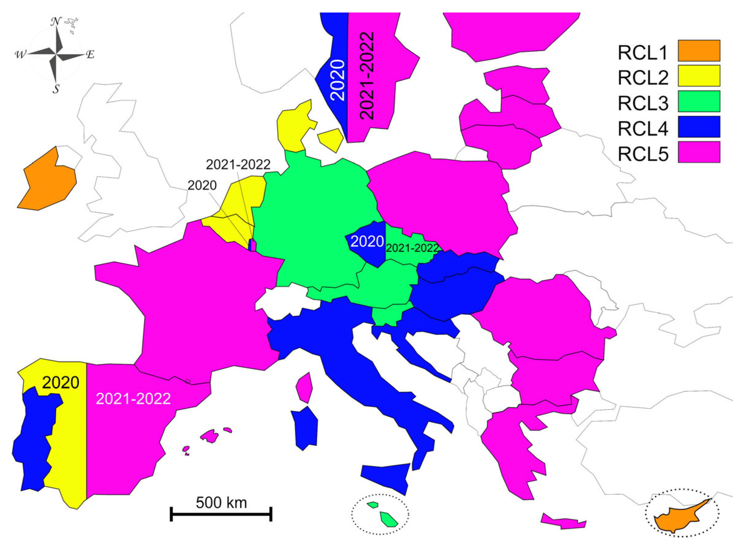
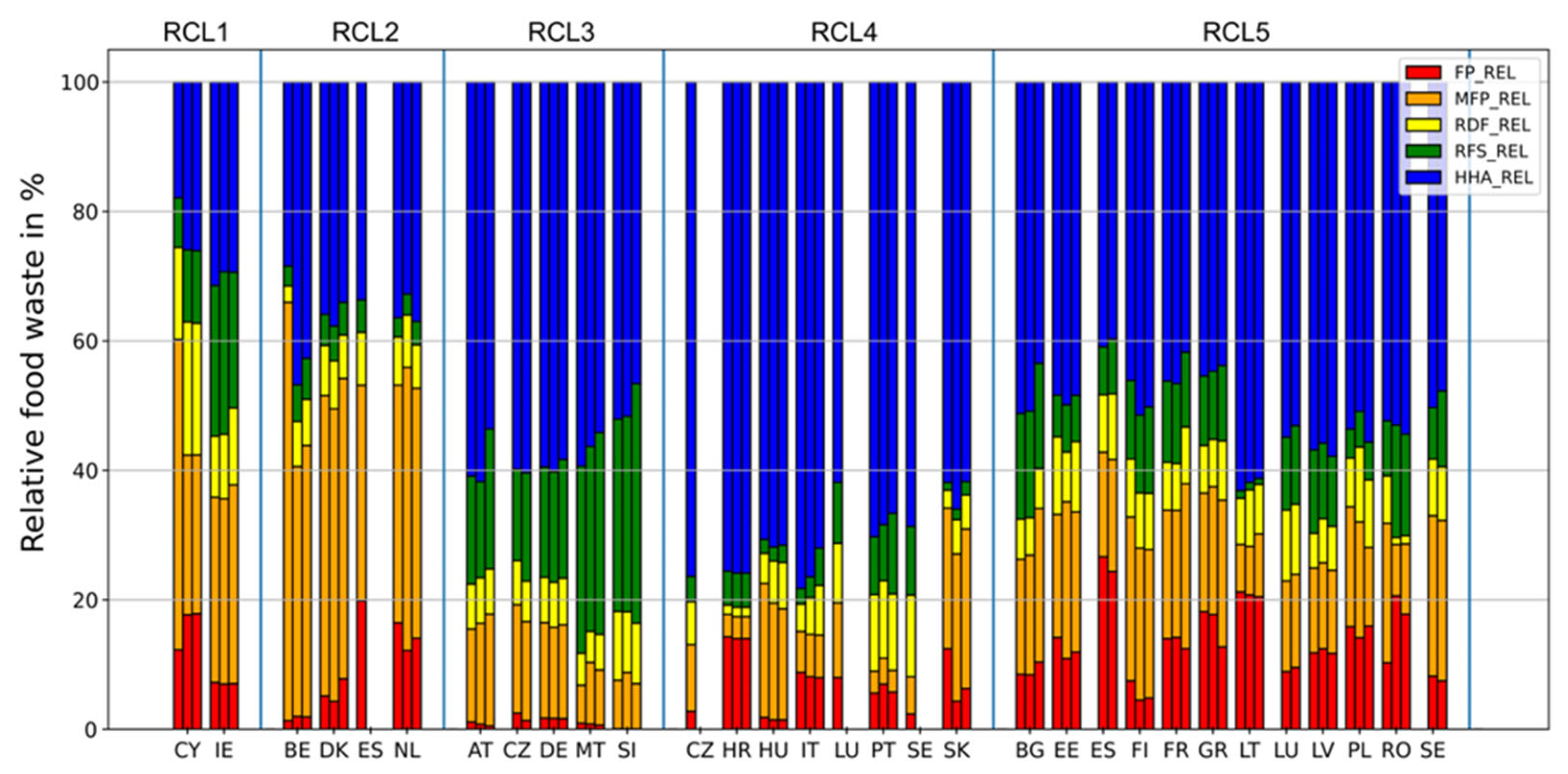
Cluster analysis was also performed on the relative food waste data. The next list presents the members of clusters in text, and in Figure 5 they are presented in a color-coded map, while Figure 6 shows the relative food waste parameters in a stacked histogram. The initial letter “R” of the cluster identifiers indicates the relative parameters.

• RCL1 (2 members): CY and IE.
• RCL2 (4 members): BE, DK, ES (2020) and NL.
• RCL3 (5 members): AT, CZ (2021, 2022), DE, MT and SI.
• RCL4 (8 members): CZ (2020), HR, HU, IT, LU (2020), PT, SE (2020) and SK.
• RCL5 (12 members): BG, EE, ES (2021, 2022), FI, FR, GR, LT, LU (2021, 2022), LV, PL, RO and SE (2021, 2022).

The analysis demonstrates that 23 out of 27 countries maintained their cluster affiliations over the three-year period. This significant stability confirms that the composition of food waste sources remains consistent despite short-term fluctuations. Moreover, similarly to the results of the absolute value-based clustering, the year 2020 is the standout year in all such cases (Spain, Czech Republic, Luxembourg and Sweden).

Table 5. Sectoral distribution of cluster centre values based on food waste relative values in percentages. Yellow background indicates the column-wise maximum.

	FP	MFP	RDF	RFS	HHA
RCL1	11.5	30.9	14.4	16.6	26.7
RCL2	8.5	43.5	6.9	4.5	36.5
RCL3	1.0	12.1	7.1	23.0	56.8
RCL4	7.0	10.7	6.5	5.2	70.5
RCL5	13.6	17.8	7.9	10.1	50.6

presents the cluster centre values for each cluster, representing the distribution of food waste relative data in different sectors. The maximum values within each column are highlighted with a yellow background. It is remarkable that each cluster features exactly one yellow cell, which means that all five clusters can be characterized by one of the relative food waste parameters. However, for all clusters except RCL1 and RCL2 the majority of waste is generated from household activities. Household food waste (HHA) alone represents 70% of the total in RCL4, showing that in these countries household activities are the dominant source of food waste production. In contrast, manufacture of food and beverages (MFP) makes up the largest portion in RCL2. RCL3 is primarily characterized by a higher proportion of food waste originating from restaurants and food services (RFS) compared to other clusters. Agricultural-origin food waste is almost 14% in RCL5, which is the highest ratio compared to the other clusters. This implies that policy interventions have to be tailored: for instance, restaurant-based interventions for RCL3 and household-based interventions for RCL4 nations.

Clustering results based on absolute and relative food waste parameters differ significantly. This is understandable, considering their distinct approaches to defining “similarity”. The purpose of research should guide the selection of the more relevant method. Absolute unit groups focus on the similarity of average food waste production among individual persons, whereas relative unit groups concentrate on the distribution of a country’s food waste production generated by various sectors. For example, in terms of relative parameters, the food waste profile of Ireland is similar to that of Cyprus, while their absolute values differ significantly. This may indicate that food waste-generating processes have a similar structure in Ireland and Cyprus, but Ireland has a greater degree of economic efficiency overall. The similar behaviour of Ireland and Cyprus in terms of relative values, despite great differences in absolute values, also shows that patterns of food waste can coincide across economies of highly different sizes.

4.3.3. Relationship Between Food Waste Clusters and the Structural Indicators

The structural (environmental, social, economic and geographical) indicators corresponding to the clusters identified in the preceding analysis were gathered, and a statistical analysis was conducted to determine which parameters present significant differences between the clusters. The Mann and Whitney U test was used to compare the distributions. Given the high number of possible relationships examined, strict significance levels were used to minimize the incidence of false-positive signals. Specifically, a p-value threshold of 0.01 was designated for “weak”, and a threshold of 0.001 was designated for “strong” connections. Considering that there are ten possible pairs with the five group (clusters), 10 significance tests were performed per parameter. For the 26 parameters examined, this amounts to a total of 260 tests, meaning that on average there will be 2.6 cases where the test incorrectly indicates a weak correlation and 0.26 cases where a false strong correlation signal will be obtained. These numbers have been verified by trial calculations involving the random dividing of the countries’ annual data into five groups.

The results of the 260 statistical tests are transparently presented in

Table 6. Indicators with significant differences between clusters, based on food waste per capita data. (Abbreviations of indicators: see Table 2). Empty columns (ACL1—ACL2 and ACL2—ACL3) are not displayed.

	ACL1—ACL3	ACL1—ACL4	ACL1—ACL5	ACL2—ACL4	ACL2—ACL5	ACL3—ACL4	ACL3—ACL5	ACL4—ACL5
AREA			<	<	<
CMR								<
COFP				>	>		>
ELET
FECH				>				<
GDP_PC				>	>	>>	>
GVAEGS		<	<<
IAF	<	<	<	<
MF
MSDR
MWG_PC		>	>	>>	>>	>	>
NSFT
POP		<	<
POPDENS					>
PPGDP				>	>	>>	>
PUKHW	>		>	<		<<		>>
REG_BOR_PC		<	<		<		<
REG_COA_PC
REG_INT_PC	>					<<	<<
REG_ISL_PC		>	>>					>
REG_MOU_PC
REG_RUR_PC		<	<
REG_URB_PC		<	<
RMRPG		<		<		<<		>
RPS_PC		<		<		<<		>>
TEA			>

and

Table 7. Indicators with significant differences between clusters based on relative food waste data.

	RCL1—RCL2	RCL1—RCL3	RCL1—RCL4	RCL1—RCL5	RCL2—RCL3	RCL2—RCL4	RCL2—RCL5	RCL3—RCL4	RCL3—RCL5	RCL4—RCL5
AREA						<	<<
CMR	<<	<<				>	>>	>	>>
COFP			>	>
ELET
FECH
GDP_PC			>	>	>	>>	>>	>
GVAEGS	<<					>
IAF	<<	<<	<<	<<	<<	<<	<<
MF							<			<
MSDR
MWG_PC						>	>	>>	>>
NSFT
POP	<<		<	<
POPDENS	<<	<<				>	>>		>>	>
PPGDP			>			>>	>>	>>	>
PUKHW						<
REG_BOR_PC			<	<		<	<<		<
REG_COA_PC	>>	>>	>>		>				<<
REG_INT_PC						<	<<	<	<<
REG_ISL_PC	>>	>>	>>	>>
REG_MOU_PC		<	<	<	<	<
REG_RUR_PC						<	<<		<
REG_URB_PC		<		<
RMRPG	<	<	<<	<<		<	<	<	<
RPS_PC							<		<<
TEA	>>	>>	>>	>>	>>	>>				<

. Columns correspond to cluster pairs, and each row is for a specific structural indicator. The cells are empty if no significant difference was found, but contain “>” or “<” signs for weak differences (0.001 < p-value <= 0.01) and “>>” or “<<” signs for strong differences (p-value <= 0.001). The direction of the relational signs indicates whether the first or the second cluster within a pair exhibits higher average values.

Table 6 presents the results for absolute food waste parameters, while Table 7 shows the results for relative food waste parameters. For instance, in Table 6 the row corresponding to “GDP_PC” has “>” symbols in the ACL2—ACL4, ACL2—ACL5 and ACL3—ACL5 columns and a “>>” symbol in the ACL3—ACL4 column. This row indicates that the per capita GDPs of cluster 2 and cluster 3 are greater than those of cluster 4 and 5. This suggests a statistical connection between per capita GDP and absolute food waste parameters. However, this is not a simple, monotonic connection. For example, cluster 3 exhibits higher average per capita GDP values compared to cluster 4, yet their total food waste production is approximately the same, with lower average total food waste in the case of cluster 3 compared to cluster 4. The difference between these two clusters can be found in the characteristics of their food waste as represented by the five parameters.

Cluster analysis reveals significant differences in social–economic parameters among the five clusters. The results presented in Table 6 suggest that food waste levels per person are strongly linked to socio-economic inequalities. The ACL1–ACL5, ACL1–ACL4 and ACL2–ACL4 cluster pairs show the most significant differences in terms of the examined parameters, with distinctions found across 10–11 structural indicators. Additionally, there is a noticeable contrast between the ACL2–ACL5, ACL3–ACL4, ACL3–ACL5 and ACL4–ACL5 clusters in terms of 6–7 distinct indicators.

Countries belonging to ACL2 and ACL3 are richer than countries in ACL4 and ACL5, as they have a higher GDP per capita and a higher purchasing power adjusted GDP per capita. In parallel, they have a higher consumption footprint index (COFP) and higher municipal waste generation (MWG_PC), showing a connection between stronger economies and higher overall waste output (not limited to food).

The poorer countries of ACL4, in contrast, have higher PUKHW (population unable to keep home adequately warm), IAF (inability to afford a meal), RMRPG (at risk of poverty) and RPS_PC (people at risk of poverty or social exclusion) values than the other clusters have, indicating severer social vulnerabilities in the countries in this group.

According to the values, there is no evident relationship between educational status (like ELET and TEA values) and the food waste per capita characterization of a country. The effect of geographical factors (region types) can be observed mainly in the case of Cyprus (ACL1).

The results in Table 6 indicate that absolute food waste patterns are linked to macro-economic strength and social vulnerability indicators. Wealthier countries, characterized by higher GDP per capita, higher municipal waste and lower deprivation indicators, form a distinct cluster. Conversely, poorer clusters exhibit greater social challenges and relatively lower waste per capita. This suggests that the extent of absolute food waste reflects broader socio-economic inequalities across the EU.

Table 7 compares the cluster results of the analysis performed using relative food waste values (% of total waste per sector). This shifts the focus from how much waste per capita is generated to which sectors dominate food waste in each country. This comparison reveals much greater differences between the individual clusters. The RCL2–RCL4 (15 differences) and RCL2–RCL5 (13 differences) cluster pairs present the most significant differences, but between the RCL1–RCL2, RCL1–RCL3, RCL1–RCL4, RCL1–RCL5 and RCL3–RCL5 cluster pairs there also high dissimilarities (9–11 cases).

Countries belong to RCL1, RCL2 and RCL3 have higher GDP per capita and purchasing power adjusted GDP per capita values than countries in RCL4 and RCL5. This suggests that sectoral distribution of food waste (e.g., manufacturing vs. households) is also influenced by national wealth. Meanwhile, RCL2 and RCL3 demonstrate a higher circular material use rate (CMR) compared to RCL1, RCL4 and RCL5. However, the amount of municipal waste (MWG_PC) is also higher in the countries of RCL2 and RCL3 than those of RCL4 and RCL5.

Significant differences exist in IAF (inability to afford a meal) and RMRPG (relative median at-risk-of-poverty-gap) values, with the best values observed in RCL1 and RCL2 and considerably higher values in RCL4 and RCL5. A significantly higher percentage of people in RCL5 countries face the risk of poverty or social exclusion (RPS_PC) compared to those in RCL2 and RCL3. RCL4 and RCL5 are predominantly characterized by household-level waste (70% in RCL4 and 50% in RCL5), indicating that food waste structure reflects social inequalities.

Tertiary educational attainment (TEA) is strongly connected with relative food waste patterns, with educational status being significantly better in countries within RCL1 and RCL2. People in rural and border regions dominate countries belonging to RCL4 and RCL5 (Eastern and Southern Europe).

To sum up, the results based on relative food waste data highlight structural and sectoral food waste differences. Wealthier clusters (RCL1, RCL2 and RCL3) tend to have higher food waste in manufacturing (RCL1 and RCL2) and restaurant services (RCL3), while in poorer clusters (RCL4 and RCL5) households are the primary source of food waste. This latter pattern may be attributed to weaker redistribution infrastructures, cultural habits and socio-economic vulnerabilities. Geographical context (e.g., rural vs. urban areas) further reinforces these patterns.

As was mentioned above, absolute and relative food waste parameters characterize the food waste production of the countries in different ways. Comparing Table 6 to Table 7 shows a significant difference: the former contains 13 strong and 47 weak connections, while in the latter there are 48 strong and 45 weak connections. This indicates that the clusterization based on relative data has a stronger relationship with the structural parameters than that based on absolute data. Uncovering the reason behind this difference can be a topic of further research, but the observation may be important in understanding the connection between food waste production and structural parameters.

5. Conclusions

The paper investigates patterns of food waste generation across the 27 EU member states between 2020 and 2022, with particular attention paid to the period of the COVID-19 pandemic. Eurostat data for five main food waste sources (primary production, food manufacturing, retail–distribution, food services and households) were analysed and compared with over twenty social, economic, environmental and geographical indicators. Correlation analysis, Principal Component Analysis (PCA) and cluster analysis were applied to identify multivariate relationships, to reveal similarities and differences and to classify countries according to their waste generation profiles.

The results indicate that the total volume of food waste in the EU remained relatively stable during the observed three years, but its composition changed significantly. Household food waste peaked in 2021 during lockdowns, while food waste originating from distribution and food services increased steadily. Principal Component Analysis revealed a clear distinction between system-level (linked to agriculture, industry and distribution) and individual-level (households and food services) food waste. Cluster analysis identified five groups of countries with largely stable food waste patterns, even under pandemic-related disruptions.

According to the results derived from absolute and relative food waste data, the level and structure of food waste are strongly linked to the economic strength and social inequalities of the EU countries. Higher-income Western and Northern European states tend to generate greater amounts of total food waste and more waste in manufacturing and food service sectors, while in Eastern and Southern Europe household food waste is the dominant factor.

Households represent the most important target for EU-wide food waste reduction policies. However, country-specific strategies are required to differentiate according to national and regional contexts. In higher-income states, efficiency improvements in the manufacturing and food service sectors should be prioritized, while in Eastern and Southern states household-level awareness campaigns and stronger social support systems should be prioritized. Future EU strategies must account for regional and social disparities in order to shift forward a more sustainable food system.

The key contribution of this paper is the demonstration that PCA facilitates obtaining a clean differentiation between system-level and individual-level drivers of food waste, which is a methodological contribution, in contrast to the descriptive analyses that are ubiquitously used in the area. Nevertheless, this approach is not without its limitations. First, relying on a three-year Eurostat dataset constrains detection capacity in capturing long-term structural changes, particularly in relation to residual effects from the COVID-19 pandemic. Second, the lack of harmonized datasets outside of the EU impedes a global comparative setting, which would situate EU trends within the wider context. Third, even though PCA and clustering were deemed useful, further statistical confirmation (e.g., robustness tests, regression or hierarchical models) could enhance the robustness of outcomes.