Article

Ecosystem Service Value Dynamics in the Yellow River Delta National Nature Reserve, China: Conservation Implications from Two Decades of Change

1
College of Resources and Environment, Shandong Agricultural University, Tai’an 271018, China
2
Yantai Institute of Coastal Zone Research, Chinese Academy of Sciences, Yantai 264003, China
3
Department of Fundamental Courses, Shandong University of Science and Technology, Tai’an 271019, China
*
Author to whom correspondence should be addressed.
Sustainability 2025, 17(20), 9291; https://doi.org/10.3390/su17209291 (registering DOI)
Submission received: 21 August 2025 / Revised: 12 October 2025 / Accepted: 16 October 2025 / Published: 19 October 2025

Abstract

Yellow River Delta National Nature Reserve plays a critical role in ecological conservation, and assessing its ecosystem service value (ESV) is essential for guiding sustainable management strategies that harmonize development and preservation. This study was motivated by the need to generate actionable insights for adaptive conservation planning in this vulnerable coastal region. We evaluated the spatiotemporal dynamics of ESV from 2000 to 2020 using a combination of remote sensing, geographic information system analyses, and statistical modeling. Primary drivers influencing the spatial heterogeneity of ecosystem service value were identified through geographical detector analysis, and future trends were projected based on historical patterns. The results revealed that (1) ESV showed a clear spatial gradient, with higher values in coastal zones, moderate values along river channels, and lower values inland, and exhibited an overall significant increase over the two decades, primarily driven by improvements in regulating services; (2) wetland area and precipitation were the most influential factors, though socio-economic elements and environmental conditions also contributed to ESV distribution; and (3) future ESV is expected to follow current trends, reinforcing the importance of current management practices. Given that the continuous increase in ESV from 2000 to 2020 was predominantly attributed to water body expansion, future conservation strategies should prioritize the protection and restoration of these water resources.

1. Introduction

Ecosystem services, as the key link between the natural environment and human society, refer to the material and non-material benefits that humans directly or indirectly obtain from the functions and processes of natural ecosystems [1,2]. Current international frameworks, such as the one proposed by IPBES, have further expanded this concept, defining it as “all the benefits or harms contributed by nature to individuals, communities, societies, nations, or humanity as a whole” (referred to as Nature’s Contributions to People, NCP) [3]. This framework emphasizes the role of diverse knowledge systems and cultural contexts in understanding ecosystem services. Meanwhile, the European Union’s Mapping and Assessment of Ecosystems and their Services (MAES) [4] has also advanced ecosystem services from a conceptual stage to practical application in spatial integration and decision support. Classified into four categories, namely, supporting, provisioning, regulating, and cultural services, they have a profound impact on human well-being [5]. The coordinated management of the multiple objectives of ecosystem services represents a significant challenge for the sustainable development of social–ecological systems, requiring adaptive trade-off choices based on different stages of socioeconomic development [5,6]. The concept of ecosystem service value (ESV) provides a quantitative measure of an ecosystem’s capacity to support human well-being and serves as a critical indicator in spatial planning and policy-making [7]. To more clearly clarify the conceptual chain from ecosystem functions to services, and further to the assessment of their values, this study constructs the conceptual framework shown in Figure 1, which systematically presents the logical connection between ES and ESV.
Land use change critically shapes the supply and spatial distribution of ecosystem services [8,9,10,11], as alterations to land cover types fundamentally drive shifts in ecosystem structure and function [12,13]. Given the central role of land in shaping ecological dynamics, precise monitoring of land use change is essential for robust ESV assessment and for achieving a sustainable balance between ecological conservation and regional development [14].
Globally, coastal wetlands are among the most productive ecosystems, delivering indispensable services such as storm buffering [15], water purification [16], and carbon sequestration [17], yet they are disproportionately threatened by human activities and climate change [18]. These global challenges underscore the critical urgency of understanding and preserving such vulnerable ecosystems. Within this international context, the Yellow River Delta National Nature Reserve (YRDNNR) serves as a critical case study. The YRDNNR, shaped by dynamic land–sea interactions, represents one of China’s youngest, most extensive, and most intact coastal wetland ecosystems [19]. This area supports a diverse bird population, providing critical habitat for rare species and serving as a vital waterfowl hotspot [20,21]. However, due to long-term natural and human-induced pressures, the ecological environment of the YRDNNR is extremely fragile [22]. The health of the wetland landscape pattern in the Yellow River Delta has declined, marked by increasing fragmentation, although it exhibits a trend of initial decline followed by a subsequent recovery [23]. Coastal wetlands exhibit moderate ecological vulnerability, which declines gradually with increasing distance inland from the shoreline [24]. Human disturbance intensity in the Yellow River Delta has been continuously increasing, exhibiting pronounced spatial heterogeneity, with the proportions of moderately, severely, and extremely severely disturbed areas steadily [25]. Against this backdrop, this study seeks to decipher the spatiotemporal evolution, drivers, and future trajectories of ESV in the YRDNNR, thereby informing conservation strategies under global environmental change. By addressing this question, we aim to advance the exploration of future development pathways for human ecological reserves under the dual pressures of climate change and human activities.
ESV assessment is a hotspot research focus in the fields of ecology and environmental science. Costanza et al. pioneered the classification of global ecosystem services into 17 sub-categories of ecosystems and employed various methods to estimate the global value, significantly advancing ESV research [26,27,28]. Their foundational work catalyzed a vital field of study, spurring the development of influential frameworks such as the Millennium Ecosystem Assessment [29]. These international initiatives have helped establish standardized methodologies for quantifying and valuing ecosystem services, which are now widely applied across a variety of ecosystems worldwide. Since then, studies on the ESV of the Yellow River Delta have become increasingly enriched [30,31,32]. However, most existing research focuses on the Yellow River Delta as a whole, while investigations specifically targeting the YRDNNR, a core area of ecological significant, remain relatively limited. Furthermore, current studies frequently employ quantitative indicators including the land use dynamic degree and land use transfer matrices, complemented by simulation models such as FLUS-Markov, to project future ESV evolution [33].
Process-based models such as InVEST, ARIES, and ECOSERV have become mainstream standard tools in the current field of ESV assessment. These models possess both the advantage of high spatial explicitness and the ability to conduct in-depth analysis of the formation mechanisms of ecosystem services. The equivalence factor method was ultimately chosen in this study, not only to address practical needs related to data availability, but more crucially due to the method’s compatibility with the specific assessment context of this research. Its core advantages are mainly reflected in two aspects: First, it exhibits prominent comprehensiveness and standardization: the method enables simultaneous assessment of multiple ecosystem services and provides a unified assessment framework. This facilitates comparative analysis of ESV results across different regions and studies, effectively avoiding the problem of incomparable results caused by differences in assessment systems. Second, it emphasizes a macro-level assessment perspective: it can accurately identify the trade-off effects and synergistic relationships between land use changes and the evolution of total ESV, helping to clearly grasp the overall change patterns of regional ecosystem services and aligning with the core needs of macro-scale research.
From the perspective of this study’s core objectives, the research aims to conduct a long-term, regional-scale assessment of ESV dynamics under past and future land use change scenarios in the YRDNNR. In this context, the advantages of the equivalence factor method in terms of result comparability, method repeatability, and multi-scenario simulation analysis are sufficient to offset its shortcomings relative to process-based models in spatial resolution. Furthermore, the equivalence factor method is already well-established in domestic ESV assessment research, with a clear technical path and strong adaptability of its parameter system. It is particularly suitable for quickly identifying the overall trends of regional ESV changes, thereby providing scientific support for formulating macro ecological conservation strategies and optimizing land use planning in the reserve.
Building on the current research landscape and existing gaps, this study focuses on the YRDNNR, analyzing ESV for the years 2000, 2005, 2010, 2015, and 2020. The methodology incorporates Theil-Sen trend analysis, the Mann–Kendall test, and the Hurst exponent to assess temporal and spatial changes. The study aims to (1) reveal the spatial distribution characteristics of ESV in the YRDNNR; (2) analyze the spatiotemporal changes in ESV in the YRDNNR; (3) explore the driving factors influencing ESV using the Geo-Detector model; and (4) predict the future ESV trends within the reserve. Based on the reserve’s conservation context, we formulated the following testable hypotheses: The spatial-temporal evolution of ESV is primarily driven by the conversion of other land types to water bodies and wetlands, a process largely attributable to ecological restoration policies. Through these analyses, this study seeks to provide scientific and strategic support for ecological conservation and management in the YRDNNR.

2. Materials and Methods

2.1. Study Area

The YRDNNR is situated in the northern part of the Shandong Peninsula, bordering the Bohai Sea to the north [34]. The region features a temperate monsoon climate, marked by distinct seasons and a pronounced concurrence of rainfall and heat [35]. The total area of the reserve is 153,000 ha, with the specific area of each functional zone as follows: the core zone covers 59,420 ha, the buffer zone 11,230 ha, and the experimental zone 82,350 ha [36]. In terms of land cover characteristics, wetlands are the dominant surface type in the region, accounting for an average of approximately 48.52%, followed by agricultural land, which accounts for an average of 20.02%. In terms of biodiversity, the region is home to 21 species of rare and endangered birds, highlighting its prominent ecological value [36]. Strategically positioned along major migratory bird routes, the reserve functions as a critical node in avian migration, providing essential stopover and habitat resources [37]. The Yellow River Delta is endowed with abundant oil and natural gas resources. As the location of Shengli Oilfield, China’s second-largest oilfield, it serves as a crucial pillar supporting the nation’s petrochemical industry system [38]. The region supports a population of over 10.53 million and has contributed 403.75 billion US dollars to the regional GDP in recent years [39]. In response to national ecological policies, the removal of 300 oil and water wells from the core and buffer zones was initiated in 2017 following an environmental inspection. This decommissioning process was carried out in phases and was fully completed by the end of 2020.
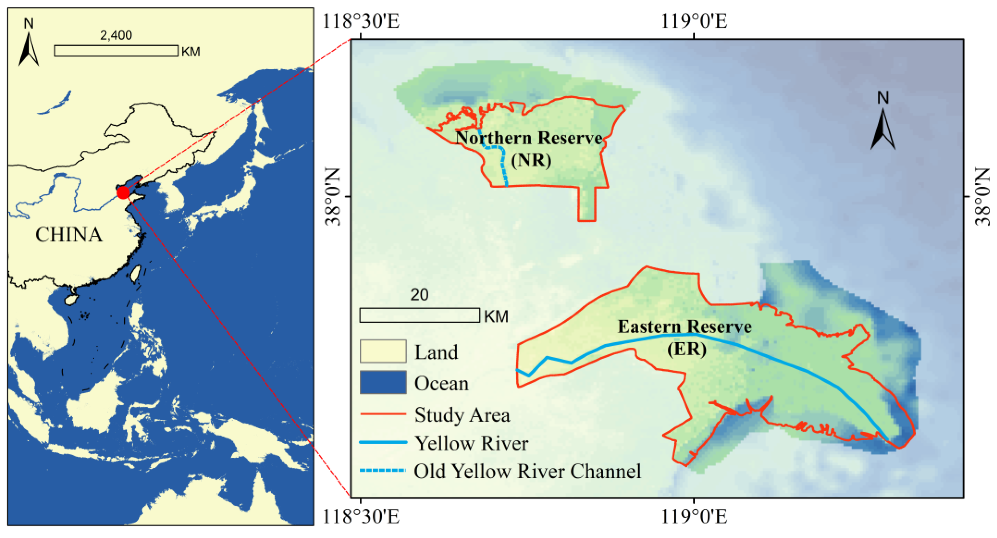
The YRDNNR consists of two sections: the Yellow River estuary and the old river channel previously used for flood diversion before 1976. These two parts referred to as the Eastern Reserve (ER) and the Northern Reserve (NR), respectively [21]. The reserve is composed of both marine and terrestrial ecosystems. However, due to the incomplete nature of the marine data and the fundamental differences in material cycling, energy flow, and species composition between marine and terrestrial systems, this study focuses solely on terrestrial ecosystems to ensure the accuracy and reliability of our assessment (Figure 2). Excluding marine ecosystems may indeed introduce a bias, as their substantial ESV is absent from our total estimate. Work such as Barbier [40] establishes that the ecosystem services provided by estuarine and coastal ecosystems (ECEs) are of extremely high value. Consequently, our terrestrial ESV is a conservative, lower-bound figure. Our focused approach prioritized methodologically sound and data-driven analysis of the terrestrial component, which is a critical and quantifiable part of the reserve’s total value. Future studies incorporating robust marine data are needed for a complete assessment.

2.2. Data Sources

The main data used in this study covers three major categories: land use, agricultural economy, and driving factors of ESV, spanning five-time nodes: 2000, 2005, 2010, 2015, and 2020, with the spatial scope covering the entire study area. Specifically, the data includes land use data and the planting area, yield, and market price data of major food crops in the study area during the same period.
To explore the driving forces behind ESV changes, we selected 8 categories of natural and socioeconomic factors by comprehensively referencing existing studies and regional characteristics [14,35]. These factors mainly include indicators of topography (DEM), climate (precipitation), vegetation coverage (NDVI), socioeconomic factors (GDP, population), and spatial distance and pattern (wetland area, distance to construction land, distance to roads), among others. For wetland area, in addition to the water bodies (Rivers and Canals, Lakes, Reservoirs and Ponds, Tidal Flats, and Riparian Beaches) from the multi-temporal land use remote sensing monitoring dataset for China (CNLUCC), we also incorporated marshland. DEM data were resampled, and their spatial resolution was uniformly adjusted to 1 km. The wetland area was directly calculated from the reclassified land use data. The variables of distance to construction land and distance to roads were computed as Euclidean distances. Details regarding the data sources and resolutions are as follows (Table 1).
The data were sourced from the authoritative Data Center for Resources and Environmental Sciences, Chinese Academy of Sciences (RESDC), and the socioeconomic data were obtained from the official National Statistical Yearbooks. While these represent the most credible and widely used data sources for research on this scale, it is acknowledged that potential uncertainties, such as the spatial resolution of imagery or inter-annual calibration in statistical reporting, persist. These uncertainties primarily influence the accuracy of provisioning services valuation, such as the estimation of crop yields. To ensure consistency and minimize their impact, uniform pre-processing and classification protocols were rigorously applied across all study periods. The findings of this study should therefore be interpreted with an awareness of these inherent data constraints.

2.3. Research Methods

2.3.1. Data Processing Flow

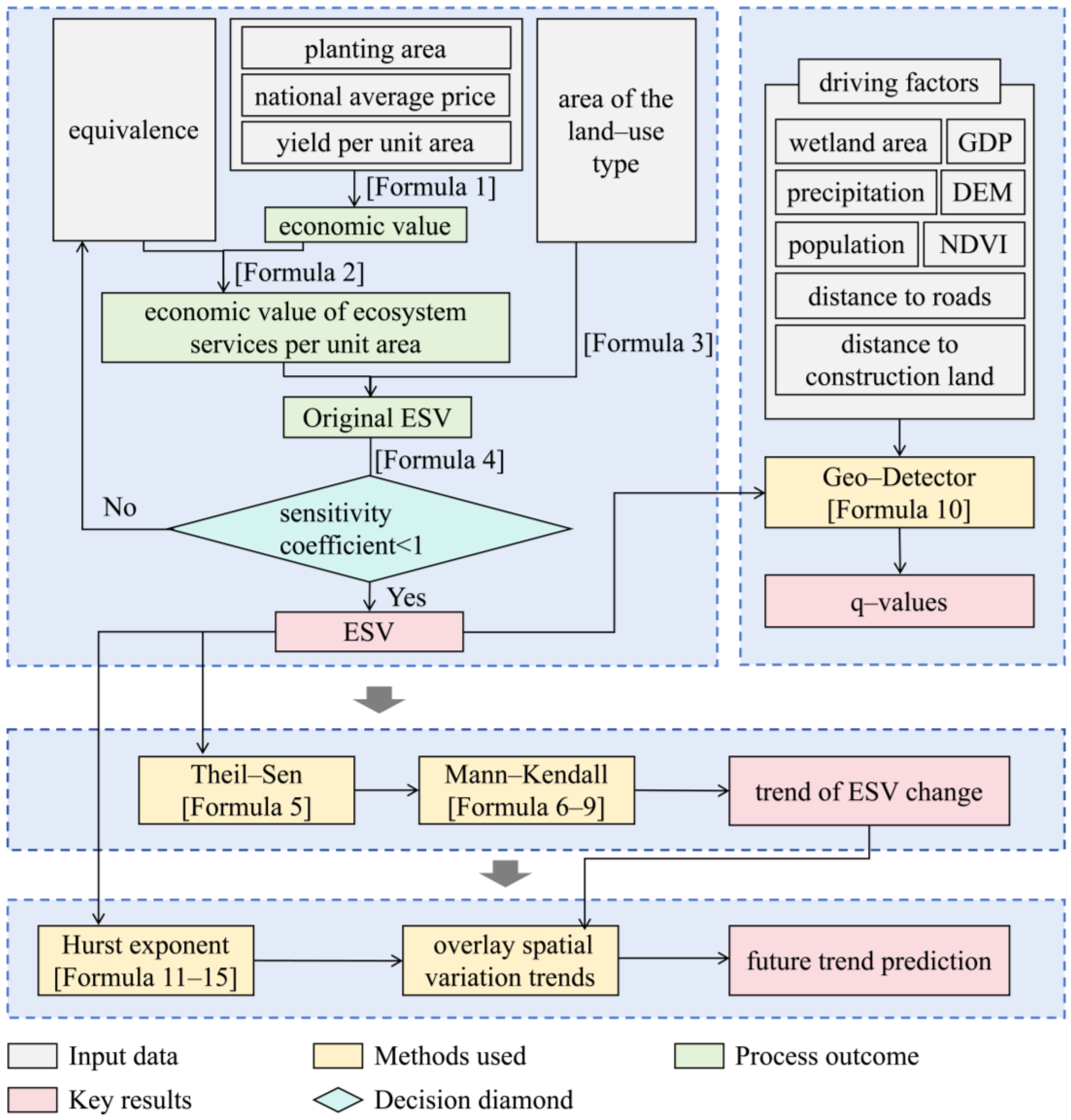
The data processing workflow centers on the research of ESV and comprises four key steps: First, by integrating basic data such as land use and equivalent factors, conduct standardized evaluation and calculation of ESV to define the core base value; Second, analyze the spatiotemporal variation trends of ESV to accurately capture the patterns of increase and decrease across different time periods and regions; Third, explore driving factors, not only identifying the causes of annual differences but also summarizing the long-term average dominant factors; Fourth, predict the future spatial distribution of ESV by coupling the Hurst exponent with the existing spatial distribution status, thereby providing a scientific basis for ecological protection and planning. The specific flow chart is shown in Figure 3.

2.3.2. ESV Calculation Methods

In this study, we adopted the equivalence factor method, primarily due to its advantages in data accessibility, suitability for macro-level assessment of ESV over long time series, and wide application in the field of ESV assessment [41,42,43]. Unlike the InVEST model, which, while capable of providing fine-grained physical quantity assessments for single services, requires high-precision parameters and data that are difficult to fully obtain in this research field, this method is more appropriate for macroscopic evaluation of ESV across long time series. The equivalence factor method offers a standardized and practical framework for regional ESV assessment and comparison. A recognized limitation of this approach, however, is its reliance on unit value factors derived from broader spatial scales, which may not fully capture the site-specific ecological complexities of the YRDNNR; additionally, it involves a degree of subjectivity in value assignments. It is therefore emphasized that the calculated ESV should be interpreted not as an absolute monetary measure, but as a robust relative estimate for tracking temporal and spatial changes within the study area.
The equivalent factor method employs a standardized quantitative framework. Based on existing equivalence factors of ecosystem service functions and combined with the economic value of agricultural products for corresponding years, it calculates the economic value of the food production service function provided by a unit area of farmland ecosystem. Subsequently, by integrating the spatial distribution areas of various ecosystems, it comprehensively computes the ecosystem service value of the study region [26]. The equivalence factor refers to a coefficient that measures the relative importance of ESV in comparison to the value of food production from farmland [44]. It serves as a standardized metric to quantify how each type of ecosystem service contributes proportionally to the economic value provided by farmland food production [12,13]. By establishing this relative importance, equivalence factors enable the conversion and aggregation of diverse ecosystem services into a comparable framework, facilitating the comprehensive valuation of ecosystem services across different spatial scales and ecological types.
For the regional applicability of the equivalence factors, instead of directly using the national unified coefficients, we targeted the modification of the equivalence factors for farmland ecosystems based on the research data of Zhang and combined with the measured regional grain yield data [45]. Based on existing research and the specific land use types within the reserve, we refined the ESV equivalents per unit area to obtain the unit-area equivalence factors (Table 2), which were then used to estimate the ESV [33,45]. The estimation was conducted using a grid-based approach, with a spatial resolution of 1 km × 1 km.
Wheat, paddy rice, corn, soybeans, and tuberous crops are the major food crops cultivated in the study area. The ESV per unit area of farmland is determined based on the principle that it is equivalent to one-seventh of the market economic value of the average grain yield per unit area [46]. This study adopts this rule, primarily based on the following considerations: The method proposed by Xie has been widely used and well-established in the academic community. The assessment results derived from this method can be effectively compared with most existing studies within the study area that adopt the same framework, this comparability advantage helps to more clearly reveal the macro-scale characteristics of ecosystem service values in the study area. Meanwhile, within the assessment framework of this study, which focuses on macro-trend analysis, the “one-seventh rule” can meet the study’s basic needs for standardized assessment processes and referable results. The calculation formula is as follows:
E a = 1 7 i = 1 n a i p i q i A
where E a is the economic value of the food production service function provided by a unit area of farmland ecosystem (US dollars per hectare); i is the type of crop; a i is the planting area of the i-th crop (hectares); p i is the national average price of the i-th crop in a given year (US dollars per ton); q i is the yield per unit area of the i-th crop (tons per hectare); A is the total planting area of all crops.
The economic value of ecosystem services per unit area in the study area is calculated using the equivalence factor in combination with the average economic value per unit area. The calculation formula is as follows:
V C = k × E a
where VC is the economic value of ecosystem services per unit area in the YRDNNR (US dollars per hectare); E a is the economic value of the food production service function provided by a unit area of farmland ecosystem (US dollars per hectare); k is the unit area equivalence factor for ecosystem services [47].
After adjusting the corresponding coefficients, the calculation formula for ESV of the nature reserve is:
E S V = S × V C i
where ESV is the total value of ecosystem services (US dollars); VC is the total economic value per unit area of the i-th type of ecosystem service (US dollars per hectare); S is the area of the land use type (hectares) [43].

2.3.3. Sensitivity Coefficient

The sensitivity coefficient quantifies the responsiveness of ESV to land use change. The reliability of the adjusted ESV results may be compromised. In order to scientifically determine the credibility of the adjusted assessment results of ESV, we introduce a sensitivity coefficient to test the interdependence between ESV and the economic value per unit area of various land use types. We adjusted the economic value per unit area of different land types by 50% to calculate the sensitivity coefficient [48], and the calculation formula is as follows:
C S = E S V b E S V a / E S V a V C b V C a / V C a
where CS is the sensitivity coefficient; E S V a and E S V b are the ESV before and after adjustment, respectively; V C a and V C b are the total economic values per unit area of different land use types before and after adjustment. When CS > 1, ESV demonstrates sensitivity to changes in VC, indicating lower confidence in VC accuracy. Conversely, when CS < 1, ESV exhibits insensitivity to VC variations, suggesting higher result credibility [41].

2.3.4. Trend of ESV Change

The combined use of the Theil-Sen median trend analysis and the Mann–Kendall (MK) test enhances robustness against measurement errors and outliers, effectively minimizing interference and enabling the scientific identification of long-term trends in time series data. This approach provides a reliable basis for analysis. The Theil-Sen trend analysis offers several advantages: it imposes no distributional assumptions on the data, exhibits robustness against missing values and outliers, and precisely identifies trend direction with high tolerance to noise [49]. The calculation formula is as follows:
β = m e d i a n x j x i j i , j > i > 1
where β is the slope used to measure the trend of ESV change; median () is the median value; i and j are time indices; x i and x j are the index values in the i-th and j-th years of the time series, respectively. When β > 0 , ESV demonstrates a long-term increasing trend; when β < 0 , ESV exhibited a downward trend over time; when β = 0 , ESV remains essentially unchanged.
The MK test is non-parametric and does not require the sample data to follow a specific distribution. Moreover, it exhibits strong robustness to outliers, making it well-suited for reliably extracting change information from time series data [49].
The calculation formula for the test statistic S in the MK test is:
S = b = 1 n - 1 a = b + 1 n s g n x b x a
where a and b are time indices; x a and x b are the index values in the a-th and b-th years of the time series, respectively; sgn () is the sign function, which is calculated as follows:
s g n x b x a = 1 , x b x a > 0 0 , x b x a = 0 - 1 , x b x a < 0
The significance of the trend is judged using Z, which is calculated as follows:
Z = S 1 f ( S ) , S > 0 0 , S = 0 S + 1 f ( S ) , S < 0
f(S) is the variance of S, which is calculated as follows:
f ( S ) = n ( n 1 ) ( 2 n + 5 ) 18
where n represents the number of data points in the sequence.
The significance level α was set at 0.05. By consulting the standard normal distribution table, the critical value Z 1 α / 2 = ± 1.96 can be determined. If the test statistic Z > 1.96 , the trend is considered to have met the significance criterion at the 95% confidence level, suggesting that the trend change in ESV is statistically significant. The classification of trend characteristics following the MK test is presented in Table 3.

2.3.5. Geo-Detector

Utilizing the Geo-Detector—a statistical model examining ESV spatial heterogeneity and its driving mechanisms [50]—this study applies the factor detector module, and the calculation formula is given as follows:
q = 1 h = 1 L N h σ h 2 N σ 2
where q ( 0 q 1 ) quantifies the explanatory capacity of individual driving factors regarding ESV’s spatial heterogeneity. The magnitude of q is proportional to the factor’s explanatory capacity for ESV spatial heterogeneity: Higher q-value reflects stronger explanatory power of the factor over ESV spatial variation, while lower q-value indicates diminished influence. L is the number of stratified area; N h is the number of samples within the stratified area h; N is the total number of samples in the study area; σ h 2 is the variance of the stratified area; and σ 2 is the variance of the entire region [51].
The Geo-Detector model is powerful for detecting spatial stratified heterogeneity and factor interactions. Its primary methodological consideration lies in the discretion needed for classifying continuous independent variables, as both the classification method and the number of categories can significantly influence the results. To ensure the robustness of the study results, we conducted a systematic comparative analysis of multiple classification methods (including quantiles and equal interval and so on) and schemes with different numbers of classes. Ultimately, we uniformly adopted the “natural breaks (Jenks)+5 classes” scheme for all driving factors: this scheme not only best aligns with the inherent distribution characteristics of the data but also achieves an optimal balance between model simplicity and explanatory power.

2.3.6. Hurst Exponent

As a fractal dimension estimator, the Hurst exponent (H), computed through rescaled range (R/S) analysis, assesses scale-invariant temporal correlations, measuring both long-memory effects and persistent behavior in stochastic processes [52]. It is important to note that the Hurst exponent indicates persistence but does not forecast the magnitude of future changes. The main calculation procedures were as follows:
Let T t be a time series, where t = 1, 2, …, n. For any integer τ greater than or equal to 1, τ = 1, 2, …, n, define the mean value series as:
T ¯ t = 1 τ t = 1 τ T t
Then, the cumulative deviation at time t is:
X ( t , τ ) = t = 1 τ ( T t - T ¯ t ) , 1 t τ
Define the range sequence R τ as:
R τ = m a x 1 t τ X ( t , τ ) - m i n 1 t τ X ( t , τ )
Define the standard deviation sequence S τ as:
S τ = 1 τ t = 1 τ ( T t - T ¯ t ) 2
Then, the Hurst exponent is:
H = l o g ( R / S ) l o g ( t )
where τ is the length of the time series; T ¯ t is the average value of the time series T t over the time scale τ ; X ( t , τ ) is the cumulative deviation of the time series T t from time point 1 to time point τ with respect to the mean T ¯ t ; R τ denotes the range of cumulative deviations within time scale τ , calculated as the difference between the maximum and minimum values of the deviations over this interval; S τ is the standard deviation of the time series T t relative to its average value over the time scale τ ; H is the Hurst exponent, where 0 H 1 .
When 0 H < 0.5 , the time series demonstrates anti-persistence, implying that future trends will likely contrast with historical patterns, and the proximity of H to 0 enhances the intensity of anti-persistent dynamics. Managers need to make advance plans for responding to trend reversals and implement adaptive dynamic management strategies. When H = 0.5 , the series behaves like a random process, indicating that past trends exert no influence on future developments, consistent with statistical independence. The uncertainty regarding the future evolution trend of ecosystem services in such areas is the highest among all regional types. Therefore, in relevant planning practices, it is necessary to focus on strengthening ecological monitoring and adjust response strategies in real time based on monitoring feedback, to better address potential risks. When 0.5 < H 1 , the time series demonstrates persistence, meaning that future trends tend to follow the direction of past trends, reflecting long-term dependence in the series. This means that for areas currently in a state of degradation, their degradation trends will persist for the long term in the absence of effective human intervention measures; in contrast, areas with good current ecological conditions exhibit greater stability in their ecosystem health status. Therefore, in spatial planning, it is necessary to place the restoration and management of continuously degrading areas at a high priority, while implementing the strictest protection for ecological function zones with high ecological stability, to ensure their long-term and stable ecosystem service supply capacity.

3. Results

3.1. Analysis of the Spatial Distribution Characteristics of ESV

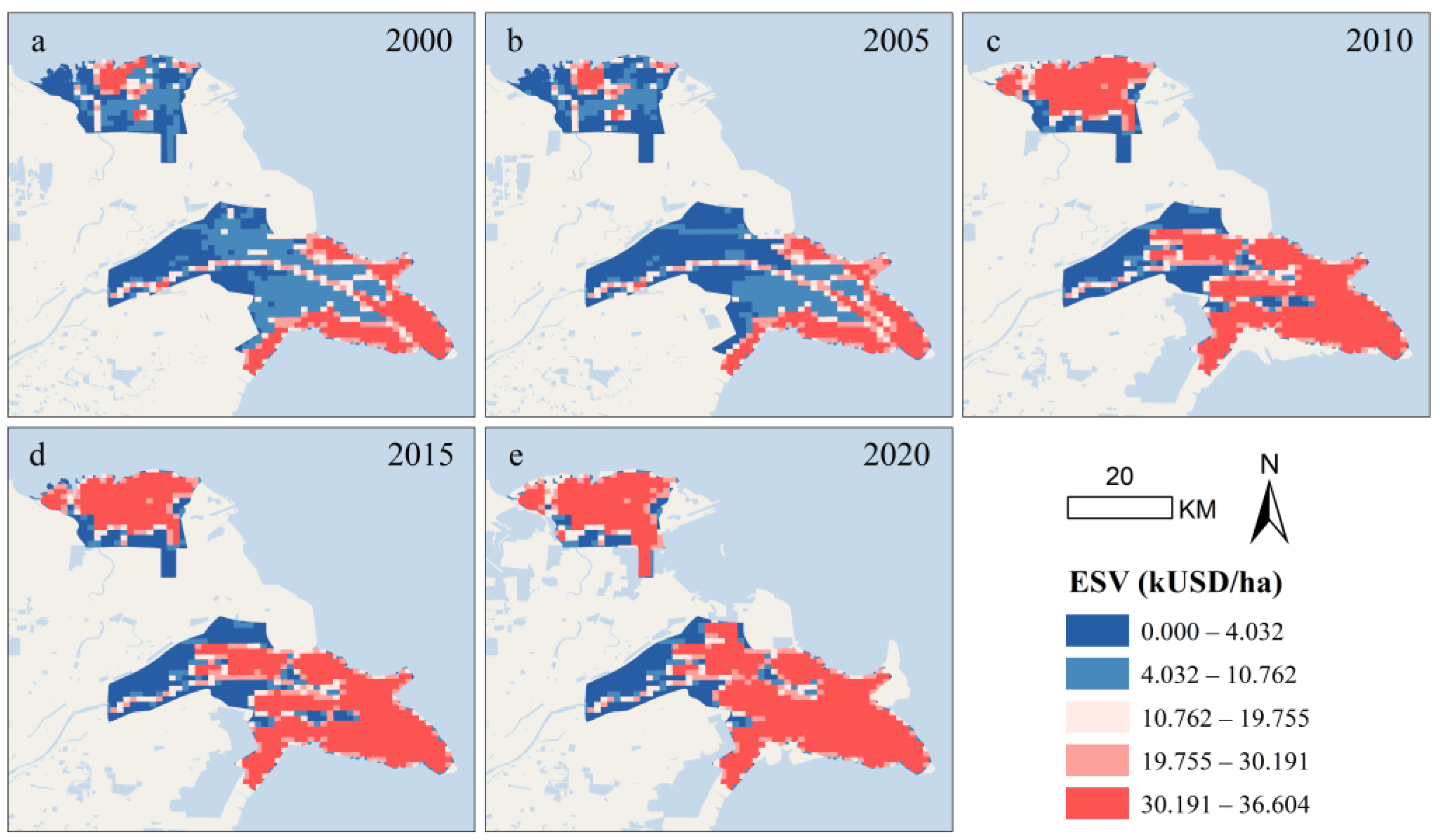
According to the calculations based on Formula 1, the economic value of the food production service function provided by a unit area of farmland ecosystem for the years 2000, 2005, 2010, 2015, and 2020 was determined to be 196.01 US dollars per hectare. In this study, ESV was classified into three tiers: low (0–10,762 kUSD/ha), medium (10,762–19,755 kUSD/ha), and high (>19,755 kUSD/ha). It can be known from the calculation results of Formula 2 and Formula 3, during 2000 to 2020, the ESV of the YRDNNR exhibited significant spatial characteristics: coastal ecosystems consistently demonstrated high ESVs, while inland areas showed relatively lower values, and riverine regions maintained intermediate levels (Figure 4). From the perspective of regional distribution, the coastal areas of ER and the northern side of NR stood out with particularly high ESVs. In these areas, the ESV per hectare exceeded 30,191.304 US dollars. In contrast, the western side of ER and the southern side of NR had significantly lower ESVs, falling below 4031.884 US dollars per hectare. Ecosystems adjacent to the Yellow River channel and its historical courses sustained moderate service values, with an average ESV of approximately 19,754.928 US dollars per hectare.
For the sensitivity analysis (Formula 4), the results (Table 4) indicated that the sensitivity coefficient (CS) for all land use types were less than 1, suggesting that the adjusted equivalent factor table for ESV from 2000 to 2020 (Table 2) was applicable for evaluating ESV within the reserve, and that the resulting calculations were robust and reliable. Overall, the CS for farmland and grassland exhibited a declining trend, implying that the accuracy of their corresponding coefficients had a progressively diminishing impact on the overall ESV of the reserve. The CS for forest and unutilized land remained consistently below 0.1, indicating that uncertainties in these land categories had a minimal effect on the ESV outcomes. In contrast, the CS for water bodies exhibited a sustained increase, rising from 0.82 to 0.99 over the study period. This indicated that for every 1% increase in the sensitivity coefficient of water bodies, the ESV of the reserve will correspondingly increase by 0.82–0.99%, highlighting a significantly greater influence compared to other land use types. Specifically, after 2015, affected by the dramatic landscape transformation, the grassland cover was reduced to an extremely low level, and its calculated CS consequently dropped below 0.005; after rounding off in accordance with the unified format of “retaining two decimal places”, this value is displayed as 0.00 in the table. Furthermore, construction land was excluded from the ESV calculation, resulting in a CS value of 0.

3.2. Analysis of the Variation Trend of ESV

3.2.1. Temporal Variation Trend of ESV

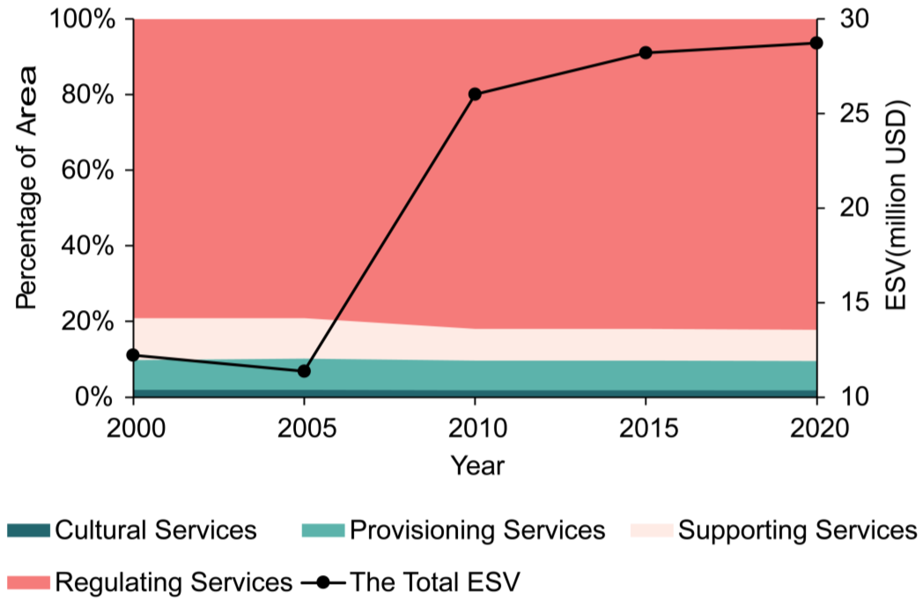
From the perspective of total ESV, the values for the years 2000, 2005, 2010, 2015, and 2020 were 1.2205 billion US dollars per hectare, 1.1363 billion US dollars per hectare, 2.6013 billion US dollars per hectare, 2.8212 billion US dollars per hectare, and 2.8725 billion US dollars per hectare, respectively. Between 2000 and 2020, the ESV of the nature reserve showed a pattern of decline in the early stage and subsequent steady growth, as shown in Figure 5. The lowest ESV was recorded in 2005, primarily due to a substantial reduction in the areas of grasslands and water bodies (Table 5). As these two ecosystems provide significant services in various aspects such as provision and regulation, their contraction directly contributed to the sharp drop in total ESV.
From the perspective of service value composition, regulating services dominated in YRDNNR, accounting for an average of 80.83%. This is primarily attributed to the extensive wetland resources within the reserve. Owing to their inherent characteristics, wetlands played a significant role in regulatory functions such as gas exchange, climate change, environmental purification, and hydrological balance. Supporting and provisioning services followed, accounting for 9.42% and 7.88%, respectively, while cultural services represented the smallest proportion at only 1.87%.

3.2.2. Spatial Variation Trends of ESV

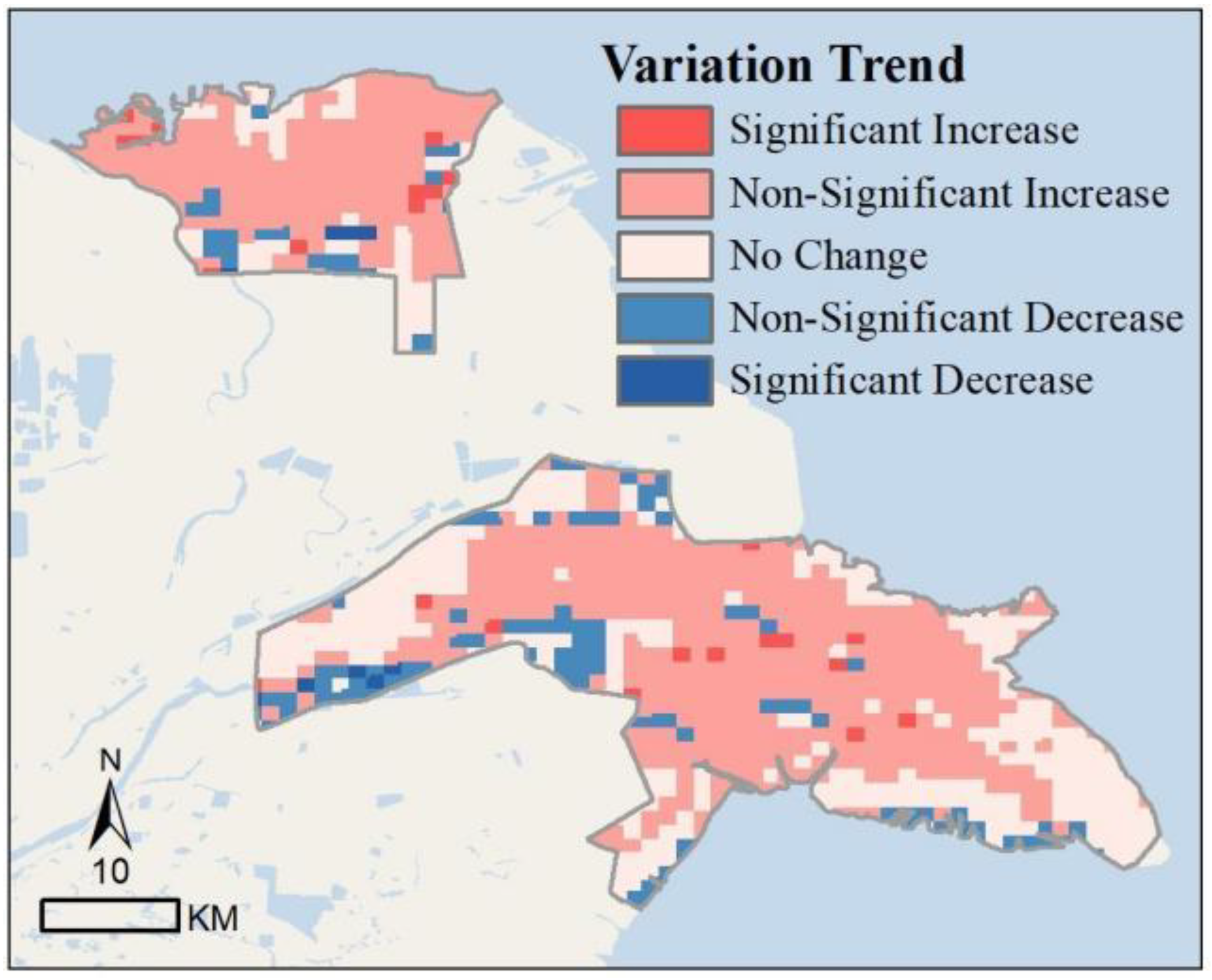
Spatially, based on the results of Formula 5–9, the overall ESV of the YRDNNR had shown an upward trend, with notable regional variations and diverse spatial characteristics (Figure 6). Among these, areas exhibiting a non-significant increase dominated the reserve, accounting for 59.24% of the area. Although the growth rate in these regions was relatively moderate, they contributed substantially to the overall increase in the reserve’s ESV. Areas with no change accounted for 28.54% of the total, predominantly located along the western and eastern coastal zones of the ER, and in the southern and northern sections of the NR. Areas with a non-significant decrease accounted for 9.46%, concentrated primarily in the southern sectors of both the ER and NR. Areas with significant increases and significant decreases were scattered throughout the reserve.

3.3. Driving Factor Analysis

We have conducted a collinearity analysis of all the impact factors. The results show that the VIF values (Variance Inflation Factor, commonly used to assess the correlation of independent variables in linear regression models) of all variables are less than 5, which is within the acceptable range (VIF < 5 indicates low collinearity risk). This demonstrates that the current system of impact factors is statistically reasonable and can be used for subsequent analyses. Using Formula 10, we calculated the q-values of each driving factor. Based on the data from 2000 to 2020, significant differences were observed in the average explanatory power (q-values) of different driving factors affecting the ESV of the reserve (Figure 7). Among them, the average q-value of wetland area reached as high as 0.98, indicating that it has persistently served as the primary determinant of ESV dynamics throughout the study period. The average q-value of precipitation was 0.22, suggesting a moderate level of explanatory influence, which ranked second only to wetland area among all factors. The average q-values for GDP, NDVI, distance to roads, and population were 0.17, 0.16, 0.15, and 0.14, respectively. Meanwhile, the average q-values of DEM was 0.12. Distance to urban land exhibited relatively lower q-values of 0.11. Overall, as a natural factor, wetland area exerted predominant control over ESV dynamics in the YRDNNR, while the effects of other factors were comparatively limited.
Through a comparative analysis of data across different time periods, it could be observed that the q-values of wetland area, GDP, NDVI, and population in relation to changes in ESV of the reserve showed a significant upward trend. This indicated that these factors had been assuming an increasingly prominent role in the dynamic changes in the reserve’s ESV, with their influence strengthening over time. In contrast, the q-value of DEM remained relatively stable with minimal fluctuation, indicating a consistent and steady impact on ESV changes. Conversely, factors such as precipitation, distance to construction land, slope, aspect, and distance to roads exhibited a gradual decline in their q-values, reflecting a weakening influence on the ESV of the reserve over time.

3.4. The Future Trend Prediction of ESV

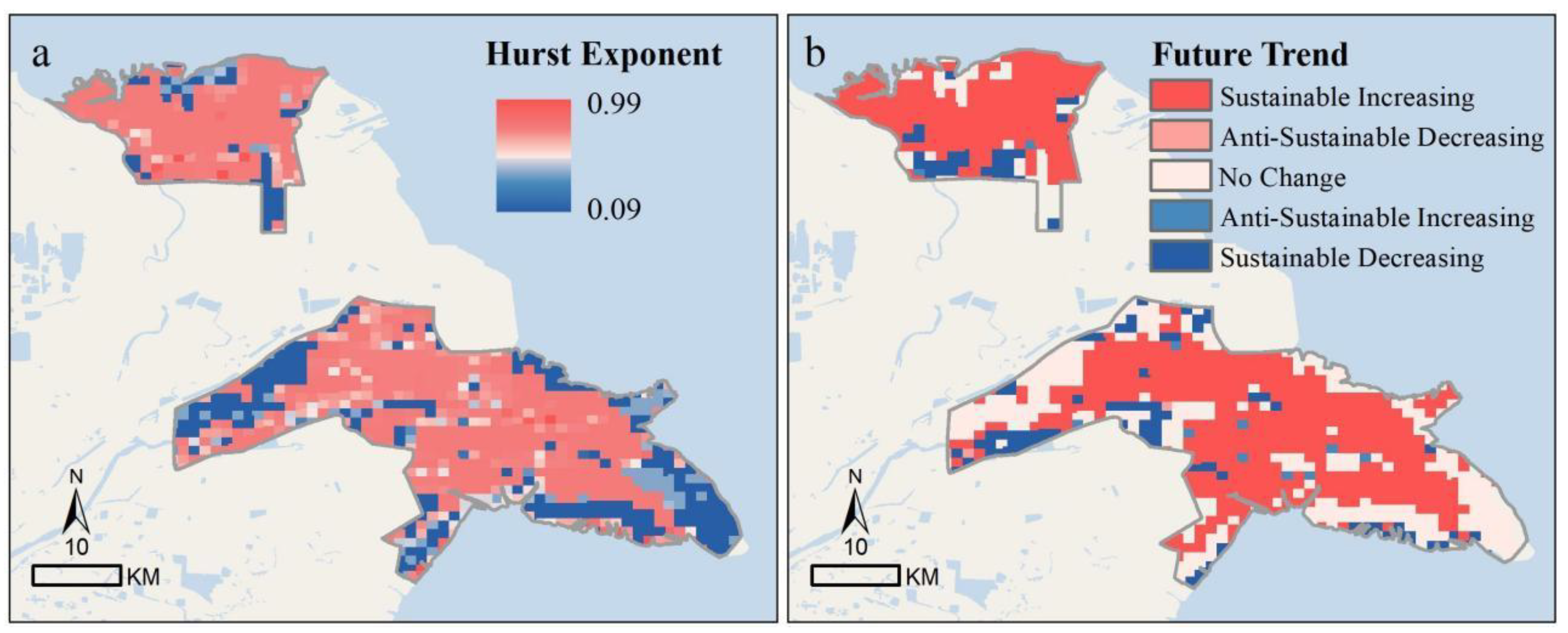
Based on Formulas 10-15, we have calculated the Hurst exponent. We conducted an overlay analysis combining the Hurst exponent and Theil-Sen trend, both of which passed the MK test, to analyze the future trends of the ESV. As presented in Figure 8 and Table 6. In the study area, the Hurst exponent (H) ranges from 0.09 to 0.99, with an average value of 0.75. Notably, 92.31% of the reserve exhibited H > 0.5, confirming the spatial predominance of persistent ESV dynamics. This suggests that, regardless of whether the current trend of the ESV is increasing or decreasing, it is highly probable that the existing trend will persist in the near future.
In the future, regions in the YRDNNR with a sustained increase in ESV account for 64.35%, the highest proportion. These areas are predominantly in the central part of ER and the northern and central regions of NR. Areas where ESV remains largely unchanged will make up 23.85% of the total area, predominantly concentrated in the western and eastern coastal regions of ER. The areas experiencing a sustained decrease in ESV will cover 10.36% of the area, mainly located in the southern parts of ER and NR. Additionally, areas with a reverse sustained increase and a reverse sustained decrease in ESV will constitute the smallest proportions, at 1.18% and 0.26%, respectively.

4. Discussion

4.1. The Spatial Distribution Characteristics of ESV

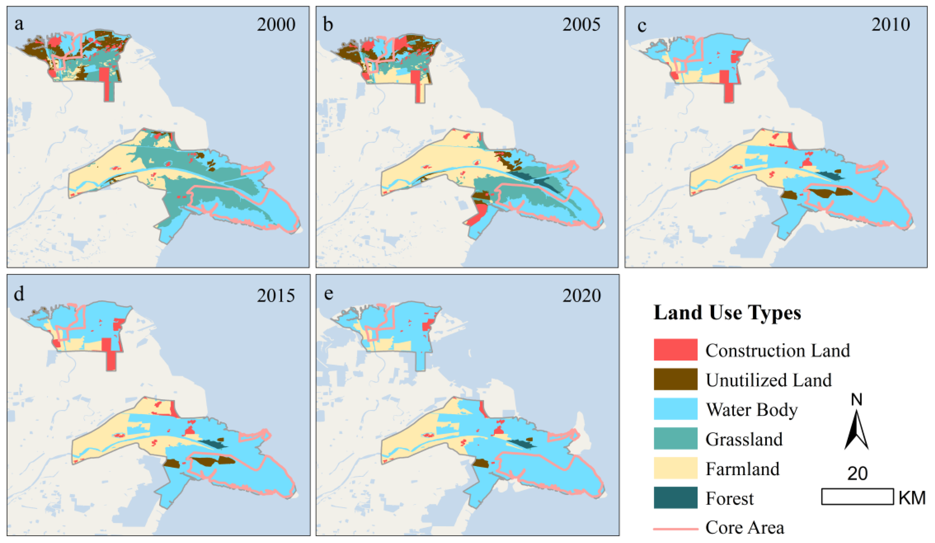
During the 2000–2020 period, the ESV of the YRDNNR exhibited a distinct spatial distribution structure, with coastal areas featuring the highest values, relatively lower values in inland areas, and moderate values in river channel areas. In this regard, Zhao et al. [35] further pointed out that the high ESV in the coastal areas of this region is mainly driven by wetland area, especially the expansion of “reservoir-pond wetlands”—a process that significantly enhances the regional water conservation and biodiversity maintenance functions. This phenomenon is consistent with previous studies where wetland-dominated zones exhibit elevated ESV due to strong regulatory functions, while farmland dominance suppresses ESV through reduced ecosystem services (Figure 9) [14,53,54]. Specifically, the low ESV in the western part of the ER and the southern NR farmland areas reflects the limited regulating services of intensive agriculture, consistent with global cropland ESV assessments [55]. This land use conversion represents a classic trade-off, where the provisioning service is enhanced at the expense of regulating and supporting services. Conversely, high ESV in eastern ER and northern NR water bodies correlate with stable aquatic ecosystems, mirroring wetland ESV patterns observed in the Qilian Mountain National Park [56]. It is the synergistic interactions among these varied land use types that have collectively shaped the unique spatial configuration of ESV in the YRDNNR.
Given this spatially heterogeneous distribution, a hierarchical and spatially differentiated governance framework is imperative. In the areas with high ESV mainly dominated by wetlands (Figure 9), which coincide with the core area of the reserve, the marine ecological redline system must be strictly enforced, with a complete prohibition on land reclamation [57,58]. Furthermore, managed flood releases from upstream reservoirs must be used to maintain the natural sedimentation rhythm on which the delta wetland’s distinctive successional trajectory depends. This conclusion should be grounded in measured data on sediment flux and accretion rates: long-term sediment monitoring at hydrological stations combined with elevation-change measurements from RSET stations can quantitatively assess the depositional effectiveness of regulated flood events [59]. Only data-driven, fine-tuned reservoir operations can ensure that flood releases genuinely enhance the ecosystem’s self-renewal capacity through natural sediment deposition.
For the inland agricultural areas with low ESV, where soil salinization further degrades ecosystem functions, we recommend an “engineering–ecological” collaborative restoration model [60]. This involves deploying subsurface drainage for desalination coupled with large-scale cultivation of salt-tolerant crops (such as suaeda salsa) [61], which can simultaneously improve soil health (a regulating service) and provide economic benefits (a provisioning service). This approach consciously manages the trade-off between intensive agriculture and ecological health by transitioning towards a more sustainable and symbiotic land use practice.

4.2. The Variation Trend of ESV

Between 2000 and 2020, the ESV of YRDNNR generally revealed an upward movement, exhibiting a growth rate of 27.694% per five years, indicating a relatively rapid increase. However, there were declines in the total ESV in both 2005 and 2015. Analysis using land use transition matrices (Table 7 and Table 8) revealed that from 2000 to 2005, a substantial amount of grassland was transformed into land use types with lower ESV, such as unutilized land, construction land, and farmland, contributing to the decline in ESV. This finding is consistent with the work of Shi et al., who found that land use changes, particularly the conversion of natural habitats to agricultural land, can lead to a decrease in ESV [62]. In addition, although the reduction in water body area is relatively small, wetlands have still experienced a slight decrease due to their unique ecological regulation function (q = 0.98). This phenomenon is consistent with the findings of Zhao et al. [35], whose study also reported that wetland area has high explanatory power for ecosystem service value (q = 0.81). Despite the small magnitude of wetland reduction, this change has still significantly lowered the total regional ESV, a result that confirms Barbier’s research conclusions regarding the high value of wetland ecosystem services [40].
These dynamics highlight the critical need for integrated land use planning and ecosystem conservation strategies in ecologically sensitive regions such as the YRDNNR. The overall recovery post-2015 likely benefits from the strengthened implementation of China’s national ecological civilization policies, such as the Ecological Redline System, which began to curb unsustainable land conversions and promote restoration. This suggests that top-down policy intervention is a potent mechanism for reversing ESV degradation. Policymakers should prioritize restricting the transformation of high ESV land types—most notably wetlands—into low-value land uses, while implementing ecological restoration programs for degraded areas [63]. Future monitoring efforts should focus on mitigating abrupt fluctuations in ESV through early-warning mechanisms for critical ecosystem transitions.

4.3. Trade-Offs, Synergies, and Integrated Management Implications

The spatiotemporal dynamics of ESV in the YRDNNR are ultimately a manifestation of trade-offs and synergies between different ecosystem services. The conversion of grassland to farmland is a clear trade-off, enhancing food provision but reducing carbon sequestration, habitat quality, and water flow regulation. Conversely, the protection and expansion of wetlands create a synergy, simultaneously enhancing a suite of services including storm buffering, carbon sequestration, water purification, and biodiversity conservation.
For managers, this implies that actions cannot be considered in isolation. Promoting salt-tolerant agriculture in low-ESV areas not only provides a new provisioning service but can improve soil regulation and create habitat, thereby creating a positive feedback loop. Conversely, any proposed infrastructure project that encroaches on wetlands must be evaluated not just for the direct loss of habitat, but for the potential collapse of multiple, synergistic regulatory services. A holistic management strategy must therefore map these service interactions to anticipate cascading effects. For instance, conserving coastal wetlands directly supports the maintenance of fisheries by providing nursery grounds, demonstrating how managing for one service can benefit another.

4.4. Study Limitations

Progress in ESV evaluation and influencing factor analysis in the YRDNNR notwithstanding, research limitations remain. Specifically, when calculating the ESV of the nature reserve, the limited availability and scope of data posed challenges in obtaining detailed information for the reserve. Therefore, the overall statistical data from Dongying City substituted for the sown area and yield of food crops, as well as the grain price. However, the ecological conditions of Dongying City may not align with those of the nature reserve. This substitution of regional data for reserve-specific data may introduce discrepancies between the calculated results and the actual ESV of the YRDNNR, potentially affecting the accuracy of the conclusions.

5. Conclusions

We have analyzed the changes in the ecosystem service value (ESV) of the terrestrial part of the Yellow River Delta National Nature Reserve (YRDNNR) from both spatial and temporal perspectives, explored the driving factors, and predicted the future trends. This research documented a continuous increase in the study area’s ESV. Detailed conclusions are presented below:
The spatial distribution of ESV demonstrates a stable and distinct coastal-inland gradient, with the highest values consistently located in coastal wetlands, the lowest in inland agricultural zones, and moderate values along river corridors. The temporal trajectory of ESV is characterized by initial decline followed by sustained growth, revealing a system highly sensitive to the conversion of key ecosystems like grasslands and water bodies.
The driving force analysis from 2000 to 2020 reveals that different driving factors have distinct average q-values for the ESV in the YRDNNR. These driving factors are ranked as follows: wetland area > precipitation > distance to construction land > Gross Domestic Product > Normalized Difference Vegetation Index > population > Digital Elevation Model > distance to roads. The YRDNNR is expected to continue its current trend into the future. Notably, the sustained ESV growth from 2000 to 2020 stemmed primarily from the continuous expansion of water bodies, underscoring the need to prioritize water body protection as a critical focus.
During the construction of the Geo-Detector model, the unique geographical environment of the study area imposed constraints on data availability, leading to incomplete environmental datasets that hindered the comprehensive identification of driving mechanisms. In the preprocessing stage for environmental variables, we conducted comparative analyses of multiple interpolation methods. Through accuracy validation, the radial basis functions (RBF) interpolation method was selected as the optimal approach for data imputation. Although this method demonstrated favorable performance in spatial data reconstruction, the interpolated results may still contain localized biases due to the scarcity of original data and regional heterogeneity, thus potentially affecting the accuracy of the driving force analysis.
Future research could incorporate a broader range of environmental and socioeconomic variables into the Geo-Detector model. Such an expansion would facilitate a more nuanced understanding of the complex interactions between natural processes and human activities in shaping the value of ecosystem services.
The comprehensive research framework applied in this study, which integrates GIS, remote sensing, the equivalent factor method, and the Geo-Detector model, demonstrates significant broad applicability. While specific equivalent factors and driving variables need to be adjusted based on the local geographical environment, its core analytical logic and model structure are transferable. Thus, this method can serve as a powerful tool for policymakers to conduct rapid ecological assessments in other regions, thereby providing support for sustainable ecosystem management.

Supplementary Materials

The following supporting information can be downloaded at: https://www.mdpi.com/article/10.3390/su17209291/s1, Table S1: The Change Curve of the Total ESV and the Proportion Diagram of Each Service. (The original data of Figure 5); Table S2: The q-value of driving force. (The original data of Figure 7).

Author Contributions

Conceptualization, S.S. and Z.M.; methodology, S.S.; formal analysis, S.S.; investigation, S.S.; resources, Z.M.; data curation, S.S.; writing—original draft preparation, S.S.; writing—review and editing, S.S., S.X. and Z.M.; visualization, S.S.; supervision, Z.M.; project administration, Z.M.; funding acquisition, Z.M. All authors have read and agreed to the published version of the manuscript.

Funding

This research was funded by the Shandong Provincial Natural Science Foundation, grant number ZR2024QD177 and Special Funds of Taishan Scholar of Shandong Province, China, grant number No. tsqnz20231205.

Data Availability Statement

The original data presented in the study are openly available in Mendeley Data at https://doi.org/10.17632/6THN49HzT8.1 (accessed on 12 October 2024).

Acknowledgments

We would like to express our gratitude to everyone who has contributed to this research, including those who have made contributions in aspects such as data collection and manuscript review.

Conflicts of Interest

The authors declare no conflicts of interest.

References

  1. Brander, L.M.; de Groot, R.; Schägner, J.P.; Guisado-Goñi, V.; van ‘t Hoff, V.; Solomonides, S.; McVittie, A.; Eppink, F.; Sposato, M.; Do, L.; et al. Economic values for ecosystem services: A global synthesis and way forward. Ecosyst. Serv. 2024, 66, 101606. [Google Scholar] [CrossRef]
  2. Costanza, R.; de Groot, R.; Sutton, P.; van der Ploeg, S.; Anderson, S.J.; Kubiszewski, I.; Farber, S.; Turner, R.K. Changes in the global value of ecosystem services. Glob. Environ. Chang. 2014, 26, 152–158. [Google Scholar] [CrossRef]
  3. Moreira, M.; Alves, J.; Frazão, L.; Gouveia, A.C.; Freitas, H. A systematic review of Nature’s Contributions to People: Impacts on science, policy, and sustainability. Sustain. Sci. 2025. [Google Scholar] [CrossRef]
  4. Czúcz, B.; Haines-Young, R.; Kiss, M.; Bereczki, K.; Kertész, M.; Vári, Á.; Potschin-Young, M.; Arany, I. Ecosystem service indicators along the cascade: How do assessment and mapping studies position their indicators? Ecol. Indic. 2020, 118, 106729. [Google Scholar] [CrossRef]
  5. Zhang, X.; Li, S.; Yu, H. Analysis on the ecosystem service protection effect of national nature reserve in Qinghai-Tibetan Plateau from weight perspective. Ecol. Indic. 2022, 142, 109225. [Google Scholar] [CrossRef]
  6. Liu, P.; Jiang, S.; Zhao, L.; Li, Y.; Zhang, P.; Zhang, L. What are the benefits of strictly protected nature reserves? Rapid assessment of ecosystem service values in Wanglang Nature Reserve, China. Ecosyst. Serv. 2017, 26, 70–78. [Google Scholar] [CrossRef]
  7. Xie, G.; Zhang, C.; Zhen, L.; Zhang, L. Dynamic changes in the value of China’s ecosystem services. Ecosyst. Serv. 2017, 26, 146–154. [Google Scholar] [CrossRef]
  8. Hasan, S.S.; Zhen, L.; Miah, M.G.; Ahamed, T.; Samie, A. Impact of land use change on ecosystem services: A review. Environ. Dev. 2020, 34, 100527. [Google Scholar] [CrossRef]
  9. Tolessa, T.; Senbeta, F.; Kidane, M. The impact of land use/land cover change on ecosystem services in the central highlands of Ethiopia. Ecosyst. Serv. 2017, 23, 47–54. [Google Scholar] [CrossRef]
  10. Turner, K.G.; Anderson, S.; Gonzales-Chang, M.; Costanza, R.; Courville, S.; Dalgaard, T.; Dominati, E.; Kubiszewski, I.; Ogilvy, S.; Porfirio, L.; et al. A review of methods, data, and models to assess changes in the value of ecosystem services from land degradation and restoration. Ecol. Model. 2016, 319, 190–207. [Google Scholar] [CrossRef]
  11. Gong, J.; Xie, Y.; Cao, E.; Huang, Q.; Li, H. Integration of InVEST-habitat quality model with landscape pattern indexes to assess mountain plant biodiversity change: A case study of Bailongjiang watershed in Gansu Province. J. Geogr. Sci. 2019, 29, 1193–1210. [Google Scholar] [CrossRef]
  12. Russo, D.; Bosso, L.; Ancillotto, L. Novel perspectives on bat insectivory highlight the value of this ecosystem service in farmland: Research frontiers and management implications. Agric. Ecosyst. Environ. 2018, 266, 31–38. [Google Scholar] [CrossRef]
  13. Feng, X.; Li, Y.; Wang, X.; Yang, J.; Yu, E.; Wang, S.; Wu, N.; Xiao, F. Impacts of land use transitions on ecosystem services: A research framework coupled with structure, function, and dynamics. Sci. Total Environ. 2023, 901, 166366. [Google Scholar] [CrossRef] [PubMed]
  14. Xue, S.; Yao, L.; Xu, Y.; Li, C. Spatiotemporal Dynamics and Driving Factors of Ecosystem Services in the Yellow River Delta, China. Sustainability 2024, 16, 3466. [Google Scholar] [CrossRef]
  15. Temmerman, S.; Horstman, E.M.; Krauss, K.W.; Mullarney, J.C.; Pelckmans, I.; Schoutens, K. Marshes and Mangroves as Nature-Based Coastal Storm Buffers. Annu. Rev. Mar. Sci. 2023, 15, 95–118. [Google Scholar] [CrossRef]
  16. Somay-Altas, M.; Sanli, E. Urban Wetlands as EcoHaven Oasis: Hydrogeochemical Insights from the Inciralti-Cakalburnu Urban Wetland (ICUW) in Izmir, Turkiye. Water Air Soil Pollut. 2025, 236, 208. [Google Scholar] [CrossRef]
  17. Hansen, V.D.; Nestlerode, J.A. Carbon sequestration in wetland soils of the northern Gulf of Mexico coastal region. Wetl. Ecol. Manag. 2014, 22, 289–303. [Google Scholar] [CrossRef]
  18. Rodríguez-Santalla, I.; Navarro, N. Main Threats in Mediterranean Coastal Wetlands. The Ebro Delta Case. J. Mar. Sci. Eng. 2021, 9, 1190. [Google Scholar] [CrossRef]
  19. Wang, X.; Lian, Y.; Huang, C.; Wang, X.; Wang, R.; Shan, K.; Pedroli, B.; van Eupen, M.; ElMahdi, A.; Ali, M. Environmental flows and its evaluation of restoration effect based on LEDESS model in Yellow River Delta wetlands. Mitig. Adapt. Strateg. Glob. Chang. 2011, 17, 357–367. [Google Scholar] [CrossRef]
  20. Huang, Z.; Lu, Y.; Meng, W.; Mo, X.; Xu, W.; Yun, H.; He, M.; Wang, Y. Study on suitability assessment of waterbird habitats along the Bohai Rim. Ecol. Indic. 2023, 150, 110229. [Google Scholar] [CrossRef]
  21. Zhang, B.; Zhang, Q.; Feng, Q.; Cui, B.; Zhang, S. Simulation of the spatial stresses due to territorial land development on Yellow River Delta Nature Reserve using a GIS-based assessment model. Environ. Monit. Assess. 2017, 189, 331. [Google Scholar] [CrossRef]
  22. Cai, Z.; Zhang, Z.; Zhao, F.; Guo, X.; Zhao, J.; Xu, Y.; Liu, X. Assessment of eco-environmental quality changes and spatial heterogeneity in the Yellow River Delta based on the remote sensing ecological index and geo-detector model. Ecol. Inform. 2023, 77, 102203. [Google Scholar] [CrossRef]
  23. Dou, X.; Guo, H.; Zhang, L.; Liang, D.; Zhu, Q.; Liu, X.; Zhou, H.; Lv, Z.; Liu, Y.; Gou, Y.; et al. Dynamic landscapes and the influence of human activities in the Yellow River Delta wetland region. Sci. Total Environ. 2023, 899, 166239. [Google Scholar] [CrossRef]
  24. Shi, H.; Lu, J.; Zheng, W.; Sun, J.; Li, J.; Guo, Z.; Huang, J.; Yu, S.; Yin, L.; Wang, Y.; et al. Evaluation system of coastal wetland ecological vulnerability under the synergetic influence of land and sea: A case study in the Yellow River Delta, China. Mar. Pollut. Bull. 2020, 161, 111735. [Google Scholar] [CrossRef] [PubMed]
  25. Chi, Y.; Shi, H.; Zheng, W.; Sun, J.; Fu, Z. Spatiotemporal characteristics and ecological effects of the human interference index of the Yellow River Delta in the last 30 years. Ecol. Indic. 2018, 89, 880–892. [Google Scholar] [CrossRef]
  26. Costanza, R.; de Groot, R.; Braat, L.; Kubiszewski, I.; Fioramonti, L.; Sutton, P.; Farber, S.; Grasso, M. Twenty years of ecosystem services: How far have we come and how far do we still need to go? Ecosyst. Serv. 2017, 28, 1–16. [Google Scholar] [CrossRef]
  27. Li, C.; Wu, Y.; Gao, B.; Zheng, K.; Wu, Y.; Li, C. Multi-scenario simulation of ecosystem service value for optimization of land use in the Sichuan-Yunnan ecological barrier, China. Ecol. Indic. 2021, 132, 108328. [Google Scholar] [CrossRef]
  28. Song, W.; Deng, X. Land-use/land-cover change and ecosystem service provision in China. Sci. Total Environ. 2017, 576, 705–719. [Google Scholar] [CrossRef]
  29. Kibria, A.S.M.G.; Costanza, R.; Gasparatos, A.; Soto, J. A composite human wellbeing index for ecosystem-dependent communities: A case study in the Sundarbans, Bangladesh. Ecosyst. Serv. 2022, 53, 101389. [Google Scholar] [CrossRef]
  30. Liu, J.; Chen, X.; Chen, W.; Zhang, Y.; Wang, A.; Zheng, Y. Ecosystem Service Value Evaluation of Saline—Alkali Land Development in the Yellow River Delta—The Example of the Huanghe Island. Water 2023, 15, 477. [Google Scholar] [CrossRef]
  31. Yan, J.; Zhu, J.; Zhao, S.; Su, F. Coastal wetland degradation and ecosystem service value change in the Yellow River Delta, China. Glob. Ecol. Conserv. 2023, 44, e02501. [Google Scholar] [CrossRef]
  32. Zhang, X.; He, S.; Yang, Y. Evaluation of wetland ecosystem services value of the yellow river delta. Environ. Monit. Assess. 2021, 193, 353. [Google Scholar] [CrossRef]
  33. Qi, B.; Yu, M.; Li, Y. Multi-Scenario Prediction of Land-Use Changes and Ecosystem Service Values in the Lhasa River Basin Based on the FLUS-Markov Model. Land 2024, 13, 597. [Google Scholar] [CrossRef]
  34. Kong, D.; Miao, C.; Borthwick, A.G.L.; Duan, Q.; Liu, H.; Sun, Q.; Ye, A.; Di, Z.; Gong, W. Evolution of the Yellow River Delta and its relationship with runoff and sediment load from 1983 to 2011. J. Hydrol. 2015, 520, 157–167. [Google Scholar] [CrossRef]
  35. Zhao, Y.; Luo, L.; Zhang, L.; Sun, J.; Lu, Z. Spatiotemporal evolution and driving forces of ecosystem service values in the Yellow River Delta. Ecol. Indic. 2025, 173, 13432. [Google Scholar] [CrossRef]
  36. Zhou, D.; Zhang, H.; Zhang, X.; Zhang, W.; Zhang, T.; Lu, C. Habitat changes in the most important stopover sites for the endangered red-crowned crane in China: A large-scale study. Environ. Sci. Pollut. Res. 2021, 28, 54719–54727. [Google Scholar] [CrossRef] [PubMed]
  37. Cui, Y.; Xiao, R.; Zhang, M.; Wang, C.; Ma, Z.; Xiu, Y.; Wang, Q.; Guo, Y. Hydrological connectivity dynamics and conservation priorities for surface-water patches in the Yellow River Delta National Nature Reserve, China. Ecohydrol. Hydrobiol. 2020, 20, 525–536. [Google Scholar] [CrossRef]
  38. Yin, Y.; Yang, R.; Song, Z.; Lu, Y.; Zhang, Y.; Zhang, L.; Sun, M.; Li, X. Simulation of wetland carbon storage in coastal cities under the coupled framework of socio-economic and ecological sustainability: A case study of Dongying city. Sustain. Cities Soc. 2024, 108, 105481. [Google Scholar] [CrossRef]
  39. Sun, B.; Wang, H.; Wu, X.; Bi, N.; Wang, G.; Wang, M.; Wang, B. Dual impacts of human activities on land cover and carbon storage in the Yellow River Delta (1986–2023). Ocean. Coast. Manag. 2025, 267, 107655. [Google Scholar] [CrossRef]
  40. Barbier, E.B.; Hacker, S.D.; Kennedy, C.; Koch, E.W.; Stier, A.C.; Silliman, B.R. The value of estuarine and coastal ecosystem services. Ecol. Monogr. 2011, 81, 169–193. [Google Scholar] [CrossRef]
  41. Gong, Y.; Cai, M.; Yao, L.; Cheng, L.; Hao, C.; Zhao, Z. Assessing Changes in the Ecosystem Services Value in Response to Land-Use/Land-Cover Dynamics in Shanghai from 2000 to 2020. Int. J. Environ. Res. Public Health 2022, 19, 12080. [Google Scholar] [CrossRef]
  42. Kindu, M.; Schneider, T.; Teketay, D.; Knoke, T. Changes of ecosystem service values in response to land use/land cover dynamics in Munessa–Shashemene landscape of the Ethiopian highlands. Sci. Total Environ. 2016, 547, 137–147. [Google Scholar] [CrossRef]
  43. Zheng, Y.; Sang, X.; Li, Z.; Zhang, S.; Chang, J. Ecological services value of ‘natural-artificial’ water cycle: Valuation method and its application in the Yangtze River Basin of China. Ecol. Indic. 2024, 158, 111324. [Google Scholar] [CrossRef]
  44. Liu, M.; Fan, J.; Wang, Y.; Hu, C. Study on Ecosystem Service Value (ESV) Spatial Transfer in the Central Plains Urban Agglomeration in the Yellow River Basin, China. Int. J. Environ. Res. Public Health 2021, 18, 9751. [Google Scholar] [CrossRef] [PubMed]
  45. Zhang, Z.; Han, L.; Feng, Z.; Zhou, J.; Wang, S.; Wang, X.; Fan, J. Estimating the Past and Future Trajectory of LUCC on Wetland Ecosystem Service Values in the Yellow River Delta Region of China. Sustainability 2024, 16, 619. [Google Scholar] [CrossRef]
  46. Yuan, D.; Du, M.; Yan, C.; Wang, J.; Wang, C.; Zhu, Y.; Wang, H.; Kou, Y. Coupling coordination degree analysis and spatiotemporal heterogeneity between water ecosystem service value and water system in Yellow River Basin cities. Ecol. Inform. 2024, 79, 102440. [Google Scholar] [CrossRef]
  47. Li, R.; Xu, Q.; Yu, J.; Chen, L.; Peng, Y. Multiscale assessment of the spatiotemporal coupling relationship between urbanization and ecosystem service value along an urban–rural gradient:A case study of the Yangtze River Delta urban agglomeration, China. Ecol. Indic. 2024, 160, 111864. [Google Scholar] [CrossRef]
  48. Xiao, J.; Zhang, Y.; Xu, H. Response of ecosystem service values to land use change, 2002–2021. Ecol. Indic. 2024, 160, 111947. [Google Scholar] [CrossRef]
  49. Bhuyan, M.; Singh, B.; Vid, S.; Jeganathan, C. Analysing the spatio-temporal patterns of vegetation dynamics and their responses to climatic parameters in Meghalaya from 2001 to 2020. Environ. Monit. Assess. 2023, 195, 94. [Google Scholar] [CrossRef]
  50. Zhang, X.; Zheng, Z.; Sun, S.; Wen, Y.; Chen, H. Study on the driving factors of ecosystem service value under the dual influence of natural environment and human activities. J. Clean. Prod. 2023, 420, 138408. [Google Scholar] [CrossRef]
  51. Chen, T.; Feng, Z.; Zhao, H.; Wu, K. Identification of ecosystem service bundles and driving factors in Beijing and its surrounding areas. Sci. Total Environ. 2020, 711, 134687. [Google Scholar] [CrossRef]
  52. Peng, J.; Liu, Z.; Liu, Y.; Wu, J.; Han, Y. Trend analysis of vegetation dynamics in Qinghai–Tibet Plateau using Hurst Exponent. Ecol. Indic. 2012, 14, 28–39. [Google Scholar] [CrossRef]
  53. Wang, W.; Xu, J.; Luan, X.; Zhang, Z. Wetland ecosystem service values in Beijing significantly increased from 1984 to 2020: Trend changes, type evolution, and driving factor. Ecol. Indic. 2024, 166, 112235. [Google Scholar] [CrossRef]
  54. Wen, X.; Wang, J.; Han, X. Impact of land use evolution on the value of ecosystem services in the returned farmland area of the Loess Plateau in northern Shaanxi. Ecol. Indic. 2024, 163, 112119. [Google Scholar] [CrossRef]
  55. Li, Y.; Shangguan, S.; Li, W.; Liu, S.; Li, Y.; Han, R.; Xu, J. Spatial–temporal distribution of farmland occupation and compensation and its impact on ecological service value in China from 1990 to 2021. Sci. Rep. 2025, 15, 14010. [Google Scholar] [CrossRef] [PubMed]
  56. Zhang, B.; Feng, Q.; Lu, Z.; Li, Z.; Zhang, B.; Cheng, W. Ecosystem service value and ecological compensation in Qilian Mountain National Park: Implications for ecological conservation strategies. Ecol. Indic. 2024, 167, 112661. [Google Scholar] [CrossRef]
  57. Chan, K.K.Y.; Ren, Z.; Liu, Y.; Song, H.; Bai, Y.; Xu, B. Land Cover Change and Fragmentation Within China’s Ramsar Sites. Remote Sens. 2025, 17, 896. [Google Scholar] [CrossRef]
  58. Guo, X.; Zhang, Y.; Guo, D.; Lu, W.; Xu, H. How does ecological protection redline policy affect regional land use and ecosystem services? Environ. Impact Assess. Rev. 2023, 100, 107062. [Google Scholar] [CrossRef]
  59. Bornman, T.G.; Schmidt, J.; Adams, J.B.; Mfikili, A.N.; Farre, R.E.; Smit, A.J. Relative sea-level rise and the potential for subsidence of the Swartkops Estuary intertidal salt marshes, South Africa. S. Afr. J. Bot. 2016, 107, 91–100. [Google Scholar] [CrossRef]
  60. Wang, J.; Ding, J.; Wang, Y.; Ge, X.; Lizaga, I.; Chen, X. Soil salinization in drylands: Measure, monitor, and manage. Ecol. Indic. 2025, 175, 113608. [Google Scholar] [CrossRef]
  61. Cao, C.; Su, F.; Song, F.; Yan, H.; Pang, Q. Distribution and disturbance dynamics of habitats suitable for Suaeda salsa. Ecol. Indic. 2022, 140, 108984. [Google Scholar] [CrossRef]
  62. Shi, Z.; Pu, W.; Dong, J. Spatiotemporal Changes of Land Use and Their Impacts on Ecosystem Service Value in the Agro-pastoral Ecotone of Northern China. Environ. Sci. 2025, 46, 2373–2384. [Google Scholar] [CrossRef]
  63. Bryan, B.A.; Gao, L.; Ye, Y.; Sun, X.; Connor, J.D.; Crossman, N.D.; Stafford-Smith, M.; Wu, J.; He, C.; Yu, D. China’s response to a national land-system sustainability emergency. Nature 2018, 559, 193–204. [Google Scholar] [CrossRef] [PubMed]
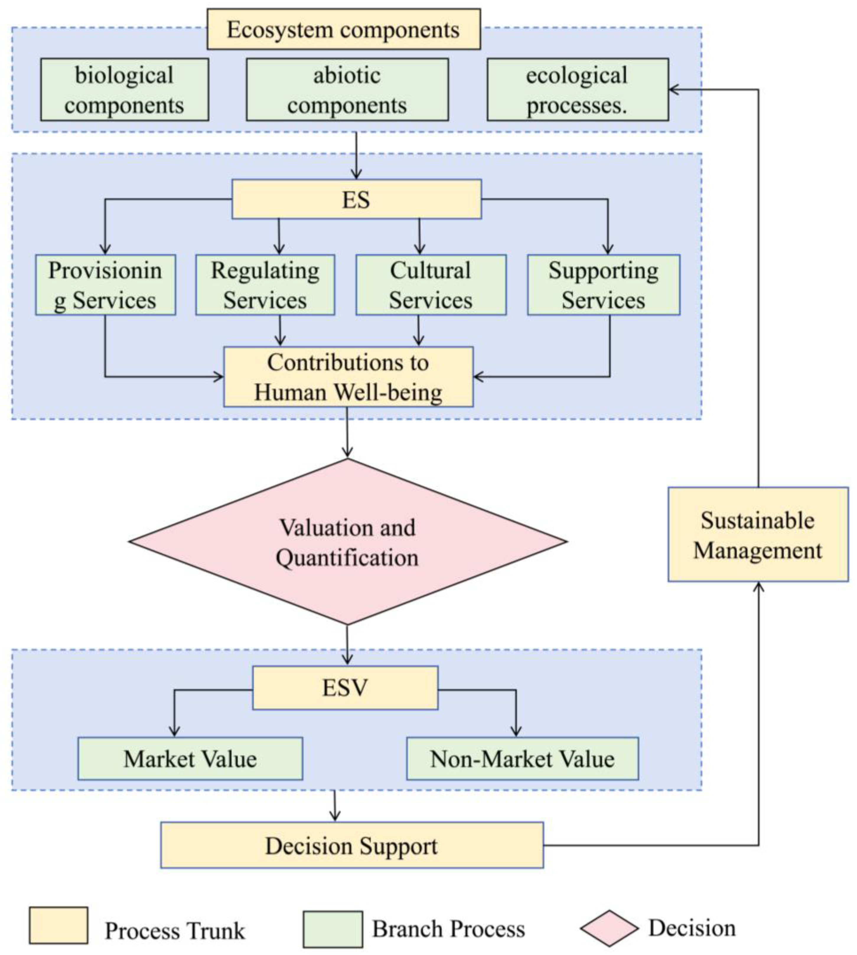
Figure 1. Conceptual framework from ecosystems to ecosystem service value assessment.
Sustainability 17 09291 g001
Figure 2. Overview of the study area.
Sustainability 17 09291 g002
Figure 3. Data processing flowchart.
Sustainability 17 09291 g003
Figure 4. Spatial distribution maps of ESV. In the figure, (ae) represent the years 2000, 2005, 2010, 2015, and 2020, respectively.
Sustainability 17 09291 g004
Figure 5. The change curve of the total ESV and the proportion diagram of each service. Note: The left vertical axis is the coordinate for the area stacked chart, and the right vertical axis is the coordinate for the line chart. Specific data can be found in Table S1 of the Supplementary Data.
Sustainability 17 09291 g005
Figure 6. The change trend of ESV from 2000 to 2020.
Sustainability 17 09291 g006
Figure 7. The q-value of each driving factor. Note: All of the interactions were significant (p value less than 0.05). Specific data can be found in Table S2 of the Supplementary Data.
Sustainability 17 09291 g007
Figure 8. The Hurst exponent and the future development trends of ESV. (a) The Hurst exponent of ESV. (b) The future development trends of ESV.
Sustainability 17 09291 g008
Figure 9. Land use types distribution maps. In the figure, (ae) represent the years 2000, 2005, 2010, 2015, and 2020, respectively.
Sustainability 17 09291 g009
Table 1. Data source and spatial resolution.
Data NameData SourcesSpatial Resolution/m
Reserve boundaryhttps://www.resdc.cn/
URL (accessed on 12 October 2024)
-
Land usehttps://www.resdc.cn/
URL (accessed on 13 October 2024)
30
Sown area and yield of food cropsShandong Statistical Yearbook-
Grain priceNational Agricultural Product Cost and Benefit Data Compilation-
NDVIhttps://www.resdc.cn/
URL (accessed on 15 October 2024)
1000
DEMhttps://www.gebco.net/
URL (accessed on 19 October 2024)
12.5
Precipitationhttps://www.resdc.cn/
URL (accessed on 27 October 2024)
1000
Populationhttps://hub.worldpop.org/
URL (accessed on 27 October 2024)
1000
GDPhttps://www.resdc.cn/
URL (accessed on 23 October 2024)
1000
Roadhttps://download.geofabrik.de/
URL (accessed on 10 April 2025)
-
Table 2. The equivalents of the ESV per unit area in the YRDNNR.
Ecosystem ClassificationUnit area ESV Equivalents
PrimarySecondaryFarmlandForestGrasslandWater BodyConstruction LandUnutilized Land
Provisioning servicesFood1.730.510.611.340.000.00
Materials0.821.180.920.750.000.00
Water0.040.610.5111.100.000.00
Regulating servicesGas1.373.883.182.730.000.04
Climate0.7311.638.406.010.000.00
Purification0.203.412.779.330.000.20
Hydrology0.557.636.16129.000.000.06
Supporting servicesSoil conservation2.104.733.883.310.000.04
Maintaining nutrient cycling0.240.370.310.260.000.00
Biodiversity0.274.323.5310.630.000.04
Cultural
services
Esthetic landscape0.060.930.763.310.000.02
Table 3. Trend characteristics of ESV.
β ZTrend of ESV
β > 0 Z 1.96 Significant Increase
Z < 1.96 Non-Significant Increase
β = 0 Z 1.96 No Change
β < 0 Z < 1.96 Non-Significant Decrease
Z 1.96 Significant Decrease
Table 4. Table of the sensitivity coefficient (CS) of ESV.
LULCYear
20002005201020152020
Farmland0.020.040.020.020.01
Forest0.000.010.000.000.00
Grassland0.160.100.000.000.00
Water body0.820.850.980.980.99
Construction land0.000.000.000.000.00
Unutilized land0.000.000.000.000.00
Table 5. ESV of each land use type (in millions of USD).
LULCYear
20002005201020152020
Farmland27.29044.31041.61645.15834.775
Forest0.00011.3806.6617.2426.536
Grassland192.450113.0590.1920.2090.203
Water body1000.217967.1182553.4722768.5242830.986
Construction land0.0000.0000.0000.0000.000
Unutilized land0.6160.6720.2360.2730.072
Total1220.5731136.5392601.7772821.4262872.572
Table 6. The prediction table of ESV’s future development trend.
Future TrendDevelopment DirectionPercentage of Area/%
Continuously increasingContinuously increasing64.35
Anti-Sustainable decreasingDecreased in the past but increasing in the future0.26
Anti-Sustainable increasingIncreased in the past but decreasing in the future1.18
Continuously decreasingContinuously decreasing10.36
No changeEssentially unchanged23.85
Table 7. The land use transfer matrix from 2000 to 2005 (hectare). Note: Matrix diagonal elements represent unchanged LULC areas, while off-diagonal elements represent LULC changes between 2000 and 2005.
LULC2005
GrasslandFarmlandConstruction LandForestWater BodyUnutilized LandTotal
2000Grassland20,184.6810,829.901324.661668.33220.021897.6436,125.23
Farmland41.1219,522.907.490.0012.7811.9419,596.23
Construction land18.2418.884781.580.009.2924.214852.20
Water body742.4580.05860.324.0331,055.2446.2832,788.38
Unutilized land9.981038.00242.030.0049.237689.379028.62
Total20,996.4731,489.747216.081672.3631,346.579669.44102,390.65
Table 8. The land use transfer matrix from 2010 to 2015 (hectare). Note: Matrix diagonal elements represent unchanged LULC areas, while off-diagonal elements represent LULC changes between 2005 and 2010.
LULC2015
GrasslandFarmlandConstruction LandForestWater BodyUnutilized LandTotal
2010Grassland29.720.000.000.000.350.0030.07
Farmland0.0024,374.6741.930.3538.910.0024,455.85
Construction land0.008.865892.360.009.070.005910.29
Forest0.460.000.00805.732.880.00809.07
Water body0.0027.1514.002.7668,209.33151.6968,404.93
Unutilized land0.000.000.110.008.972771.352780.44
Total30.1824,410.685948.40808.8468,269.512923.04102,390.65
Disclaimer/Publisher’s Note: The statements, opinions and data contained in all publications are solely those of the individual author(s) and contributor(s) and not of MDPI and/or the editor(s). MDPI and/or the editor(s) disclaim responsibility for any injury to people or property resulting from any ideas, methods, instructions or products referred to in the content.