Water Quality Prediction Model Based on Temporal Attentive Bidirectional Gated Recurrent Unit Model

Abstract

Water pollution has caused serious consequences for human health and aquatic systems. Therefore, analyzing and predicting water quality is of great significance for the early prevention and control of water pollution. Aiming at the shortcomings of the Gated Recurrent Unit (GRU) water quality prediction model, such as the low utilization rate of early information and poor deep feature extraction ability of the hidden state mechanism, this study combines the temporal attention (TA) mechanism with the bidirectional superimposed neural network. A time-focused bidirectional gated recurrent unit (TA-Bi-GRU) model is proposed. Taking the actual water quality data of the water source reservoir in Xiduan Village as the research object, this model was used to predict four core water quality indicators, namely pH, ammonia nitrogen (NH₃N), total nitrogen (TN), and dissolved oxygen (DOX). Predictions are made within multiple time ranges, with prediction periods of 7 days, 10 days, 15 days, and 30 days. In the long-term prediction of the TA-Bi-GRU model, its average R² was 0.858 (7 days), 0.772 (10 days), 0.684 (15 days), and 0.553 (30 days), and the corresponding average MAE and MSE were both lower than those of the comparison models. The experimental results show that the TA-Bi-GRU model has higher prediction accuracy and stronger generalization ability compared with the existing GRU, bidirectional GRU (Bi-GRU), Time-focused Gated Recurrent Unit (TA-GRU), Convolutional Neural Network-Long Short-Term Memory (CNN-LSTM) and Deep Temporal Convolutional Networks-Long Short-Term Memory (DeepTCN-LSTM) models.

1. Introduction

In recent years, with the continuous acceleration of urbanization, industrialization and the rapid improvement of economic level, domestic sewage, industrial sewage and farmland drainage will have a great impact on the water quality environment [1,2,3]. The increasing pollution and degradation of water resources will pose a threat to human survival, and the post-treatment of water pollution is difficult, so the prevention and control of water pollution pay more attention to prevention [4]. In order to reduce water pollution effectively and prevent it in time, the accuracy of water quality prediction becomes very important [5].

With the continuous development of information technology, many traditional machine learning models have been applied to water quality models [6]. For example, artificial intelligence neural Network (ANN) [7,8], Support Vector Machine model (SVM) [9,10], Adaptive Neural Fuzzy Reasoning System (ANFIS) [11,12], gray system [13] and autoregressive composite moving average (ARIMA) are commonly used modeling method [14].

However, in the face of the state and characteristics of water quality data with periodic changes over time, the former methods have poor generalization ability, lack of memory of historical input data, and low accuracy for long-term prediction [15,16]. Traditional machine learning models are no longer suitable for the prediction of complex models, and deep learning has gradually become the mainstream of prediction.

Recurrent neural networks (RNN), as an important branch of deep learning, can predict the state of the next moment based on the information of the previous moment by adding memory functions, and have shown application potential in water quality time series prediction [17,18]. However, RNNS have problems such as vanishing or exploding gradients, making it difficult to capture long-distance temporal dependencies [19,20,21,22]. Wongburi [23] also confirmed this limitation in his research on water quality prediction in sewage treatment plants. He found that standard RNN are difficult to handle both short-term fluctuations and long-term trends simultaneously. By introducing long short-term memory (LSTM) cells to construct the RNN-LSTM model, potential disturbances during operation were successfully detected. The effectiveness of the gating mechanism in addressing the inherent defects of RNNS has been verified. The gated recurrent unit (GRU) developed on the basis of RNN integrates short-term and long-term memory through a gated system, which to a certain extent alleviates the vanishing gradient problem [24,25]. Li et al. [26] applied GRU to the prediction of dissolved oxygen (DOX), achieving higher accuracy than traditional RNNS, demonstrating its superior performance and generalization ability in water quality prediction. However, the hidden state mechanism of a single GRU model has a low utilization rate of historical information, limited feature extraction ability, and is prone to interference from noise features as the time series increases, resulting in a decrease in accuracy. The attention-enhanced GRU (attention-GRU) proposed by Niu et al. [27] highlights key information by assigning feature weights, but still fails to solve the problem of insufficient utilization of historical information. To break through the bottleneck of a single model, researchers have begun to explore hybrid deep learning frameworks. The EEMD-MLR-LSTMNN multivariable prediction model constructed by Eze et al. [28], through the integration of ensemble empirical mode decomposition and machine learning, confirmed that the combined model can complement each other’s advantages to make up for the shortcomings of a single model and significantly improve the prediction effect of complex water quality scenarios. Similarly, Xu [29] combined the Convolutional Neural Network (CNN) with LSTM, leveraging the spatial feature extraction capability of CNN to enhance local correlations, and then capturing temporal dependencies through the memory units of LSTM. The results indicated that this combined structure could more accurately identify the dynamic patterns of water quality changes. Meanwhile, in response to the issue of insufficient utilization of historical information, researchers have attempted to adopt a bidirectional stacking structure to enhance performance. The bidirectional gated recurrent unit (Bi-GRU) model established by Li et al. [30] has been confirmed through comparative experiments that its performance is superior to that of the unidirectional GRU model and it can provide complete historical and future information for each point in the input sequence [31,32,33,34].

This paper proposes a model named TA-Bi-GRU, which incorporates the temporal attention mechanism (TA) into the Bi-GRU model and combines the advantages of the above-mentioned models. The main framework of this article is: (1) Interpolation and normalization preprocessing of water quality data; (2) Utilize the TA mechanism to assign weights to the input features and filter out useless information; (3) Utilize Bi-GRU to enhance features from two directions and capture long-term dependency states; (4) Then, the results of different prediction periods were compared with those of GRU, Bi-GRU, TA-GRU, CNN-LSTM, and DeepTCN-LSTM to prove the superiority of the TA-Bi-GRU model.

2. Study Area and Data

2.1. Study Area Profile

This study takes the Xiduan Village Reservoir in Shanzhou District, Sanmenxia City, Henan Province as the research object. The reservoir is located on the northeastern edge of the Loess Plateau, with geographical coordinates ranging from 111°20′~112°00′ E, 34°30′~34°35′ N, It is a medium-sized regulating reservoir of the Huaipa Yellow River Water Lifting Project and also one of the key water conservancy projects in Henan Province. The topography of the reservoir area is influenced by the landform of the Loess Plateau, presenting an overall undulating feature of being higher in the northwest and lower in the southeast. According to the Digital elevation Model (DEM) monitoring, the elevation range around the reservoir area is 226 to 1454 m, while the reservoir itself controls a drainage area of 38.4 square kilometers, with a total storage capacity of 29.7 million cubic meters. The average elevation of the lakebed is approximately 8 to 10 m. The average water depth is 3.2 m and the maximum water depth is 5.8 m. As the main centralized drinking water source of Mianchi County, this reservoir also undertakes the functions of water supply for the surrounding industries, irrigation for 12,000 mu of farmland and ecological water replenishment for the downstream river. Its water source replenishment mainly relies on the water lifted by the Yellow River and the water convergence around the reservoir area. There are no large natural tributaries flowing in, but there are five small agricultural irrigation drainage channels. It is a key hub connecting the water supply for “life-production-ecology” in the region.

The population growth and the expansion of facility agriculture around the Xiduan Village Reservoir have led to the reclamation of sloping land, the runoff of chemical fertilizers and pesticides, and the discharge of untreated sewage into the lake. As a result, the levels of nutrients and organic pollutants in the reservoir area have risen, posing a risk of eutrophication. According to the monitoring from 2020 to 2022, the average TN value was 0.982 mg/L, close to the Class III limit of the “Surface Water Environmental Quality Standards”. The NH₃N value rose sharply to 0.55 mg/L during the rainy season, and in 2021, the local DOX was lower than 5 mg/L. The stability of water quality is being challenged. Based on this, this study selects DOX, pH, NH₃N, and TN as core indicators: Academically, the four are internationally recognized water quality parameters. DOX reflects the self-purification and ecological activity of water bodies, pH affects the form of pollutants, NH₃N is a marker of domestic and agricultural pollution, and TN indicates eutrophication, covering the “physical-chemical-ecological” dimensions. At the local level, NH₃N represents sewage input, TN corresponds to fertilizer loss, DOX warns of algal blooms and oxygen deficiency, and pH ensures the safety of drinking water. It can accurately capture changes in water quality and provide a basis for the protection of water sources. The spatial distribution characteristics of the Xiduancun Reservoir are shown in Figure 1.

2.2. Data and Processing

2.2.1. Dataset Condition

The experimental data of this study are derived from the Shuiyuan Reservoir in Xiduan Village, Henan Province. All water quality data were collected daily through the automatic water quality monitoring station (model: YSI EXO2 multi-parameter water quality monitoring station) set up in the reservoir area. The collection period was from 1 January 2020 to 2 March 2022. The main monitoring indicators were dissolved oxygen (DOX), pH, ammonia nitrogen (NH₃N), and total nitrogen (TN), and a total of 785 valid samples were obtained. To ensure the accuracy of the data, the monitoring system strictly conducts quality control in accordance with the “Technical Specification for Automatic Water Quality Monitoring”: The sensors are comprehensively calibrated every quarter. DOX uses saturated sodium sulfite solution for zero-point calibration, and pH uses standard buffer solutions with pH values of 4.01, 7.00 and 10.01 for range calibration. The reading deviations of NH₃N and TN are verified by replacing the original factory calibration reagents. To ensure the validity of the data, the dataset was subsequently divided into a training set (the first 635 samples) and a test set (the last 150 samples) in an 8:2 ratio. The training set was used for model weighting and bias optimization, while the test set was only used to evaluate the generalization performance of the model after training. Among them, the original time series characteristics of the four indicators are shown in Figure 2. This figure visually presents the fluctuation trends of each water quality parameter during the monitoring period from 1 January 2020 to 2 March 2022, clearly reflecting the original change state of the data.

The statistical characteristics of the above water quality data are quantitatively summarized in

Table 1. Descriptive statistics of water quality data.

Index	Min	Max	Mean	SD
DOX	5.5	12.05	8.933	1.320
NH3N	0.03	0.55	0.158	0.078
pH	6.79	8.94	8.25	0.420
TN	0.38	2.21	0.982	0.251

, covering the minimum value (Min), maximum value (Max), average value (Mean), and standard deviation (SD) of each indicator, providing a basic reference for subsequent data distribution analysis and model training.

2.2.2. Data Processing

(1) Value processing is missing. During the data collection period, due to factors such as quarterly equipment calibration and short-term power outages caused by extreme weather, the water quality data of Xiduan Village Reservoir was missing for some days in April and October 2020 and March and July 2021. After statistics, a total of 32 missing samples were found, accounting for 4.1% of the total valid data (785 samples). To verify whether the missing mechanism introduces bias, we conducted the Little’s missing at random (MCAR) test on the dataset, and the test results are shown in

Table 2. Little’s MCAR test results.

Chi-Square Value	Degrees of Freedom	p-Value	Accept/Reject the Null Hypothesis
0.0556	6561	1.0	Accept

.

As shown in Table 2, the test p value is 1.0, which is greater than the significance level of 0.05. Accepting the null hypothesis of completely random data missing indicates that the missing values of water quality data at all monitoring points are not affected by other observed values (such as measured values of DOX, NH₃N, etc.), and the subsequent filling process will not introduce systematic bias. Based on this, this study adopts the third-order Lagrange interpolation method to fill in the missing values: compared with linear interpolation and polynomial interpolation, this method has lower computational complexity and higher accuracy, and is suitable for the continuous characteristics of reservoir water quality time series data. When interpolating, polynomials are constructed only based on 3 to 5 consecutive day-scale samples before and after the missing points. This approach not only avoids the problem that low-order interpolation cannot fit the fluctuations in water quality, but also prevents the Runger phenomenon when interpolating high-order polynomials (with the number of nodes ≥ 7), which could cause severe oscillations near the endpoints and increase errors.

The error term formula of Lagrange interpolation is

$$R_{n }(x)={\displaystyle \frac{f(n+1)(\xi )}{(n+1)!}}\cdot {\omega }_{n+1} (x)$$

(1)

Here, n represents the degree of the interpolation polynomial in this study, and $f(n+1)(\xi )$ is the (n + 1) th derivative of the time series function of the water quality index at a certain point $\xi$ within the interval $(t_i-2,t_i+2)$; ${\omega }_{n+1} (x)$ is the basis function product term of the interpolation node. Based on the data characteristics of this study, the value of this error term is extremely small. After estimation, the interpolation errors of indicators such as DOX and pH are all less than 0.05 mg/L or 0.02 pH units, which are far below the allowable error range of water quality monitoring data and will not interfere with the accuracy of subsequent model training.

(2) Normalized Processing. To prevent the model from experiencing convergence failure due to outliers and enhance the accuracy and stability of the model, the sample data was normalized. This normalization process transformed the data to be within the range [0, 1]. The method employed for this was the Min–Max normalization technique. Among them, to avoid using full dataset normalization to make the model know the extreme values of the test set in advance, this study follows the principle of first dividing the dataset and then normalizing it separately, ensuring the objectivity and authenticity of the subsequent model evaluation results.

3. Model Construction

3.1. Gated Recurrent Unit (GRU)

Gated Recurrent Unit (GRU) is a recurrent neural network structure based on a gating mechanism, and is a common type of RNN network structure [35]. Similarly to the LSTM model, GRU reduces the input and forget gates, and uses only update and reset gates. These gates are combined into a single gate control unit, which can use the same gate to complete the forgetting and memory of information. Additionally, the cell state and hidden state are integrated, reducing the complexity of the model and improving computational efficiency. This prevents gradient explosion or vanishing defects during LSTM backpropagation [36,37,38].

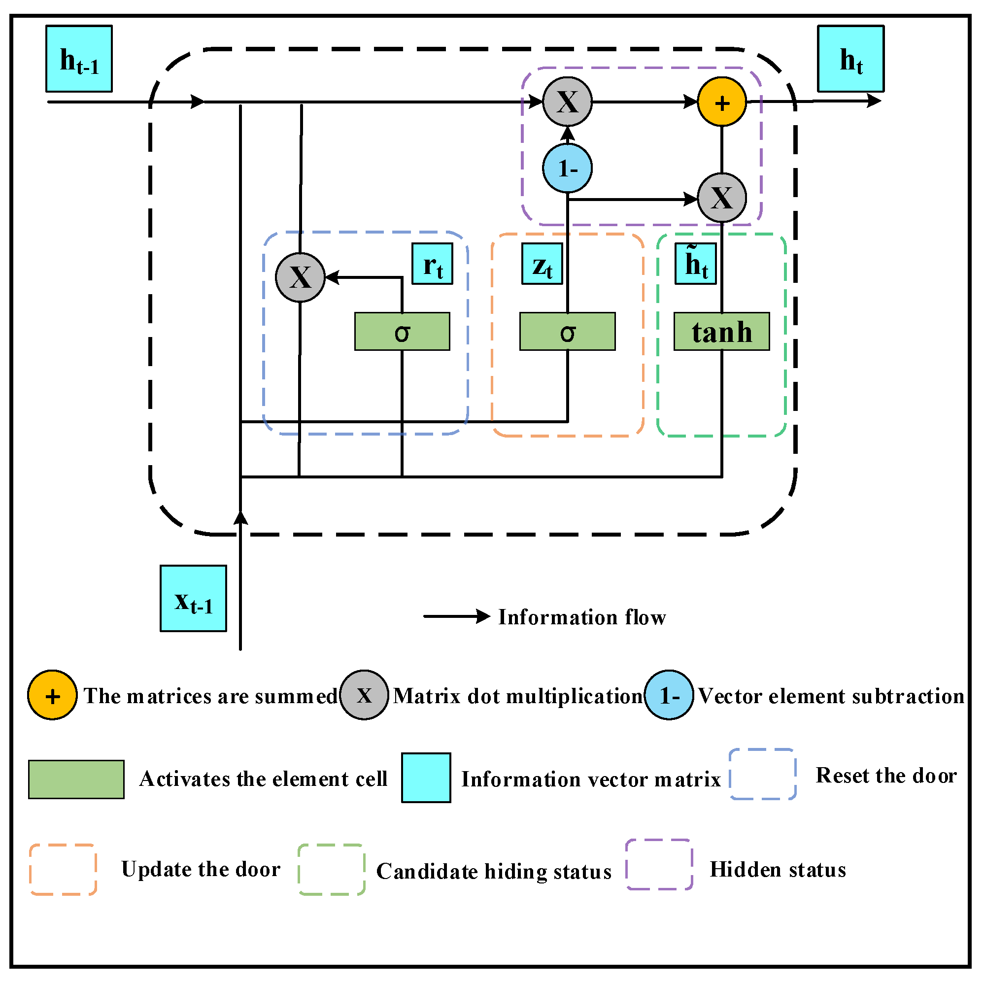
The role of the Reset Gate is to control how the input from the current moment and the hidden state from the previous moment are used to generate a new candidate hidden state. The reset gate can decide to ignore some information from the previous moment, allowing the capture of a different context. The Update Gate is a value calculated using the sigmoid function. It indicates how much of the network’s state information from the previous time and input information from the current time needs to be retained when calculating the state information for the current time. The model structure is shown in Figure 3.

The formula for calculating each parameter in the GRU network diagram is as follows:

$$z_t=\sigma (W_z\cdot [h_{t-1},x_t])$$

(2)

$$r_t=\sigma (W_r\cdot { [\mathrm{h}}_{t-1},x_t])$$

(3)

$$\begin{array}{c}{\tilde{h}}_t=\tanh \left(W_{\tilde{h}}\left[r_t\cdot h_{t-1},x_t\right]\right)\end{array}$$

(4)

$$\begin{array}{c}{h}_t=\left(1-z_t\right)\cdot h_{t-1}+z_t\cdot {\tilde{h}}_t\end{array}$$

(5)

In the above formula, $x_t$ represents the input at the current moment t. $h_{t-1}$ is the activation value output by the hidden layer of t−1 at the previous moment; $z_t$ and $r_t$ are the outputs of the reset gate and update gate at the current moment t, respectively. ${\tilde{h}}_t$ represents the candidate hidden layer output at time t, and $h_t$ is the final hidden layer output at time t (historical information is retained through $h_{t-1}$, and new information is updated through ${\tilde{h}}_t$); $W_z$, $W_r$, and $W_{\tilde{h}}$ are the corresponding learnable weight matrices, respectively.

3.2. Bi-Directional GRU (Bi-GRU)

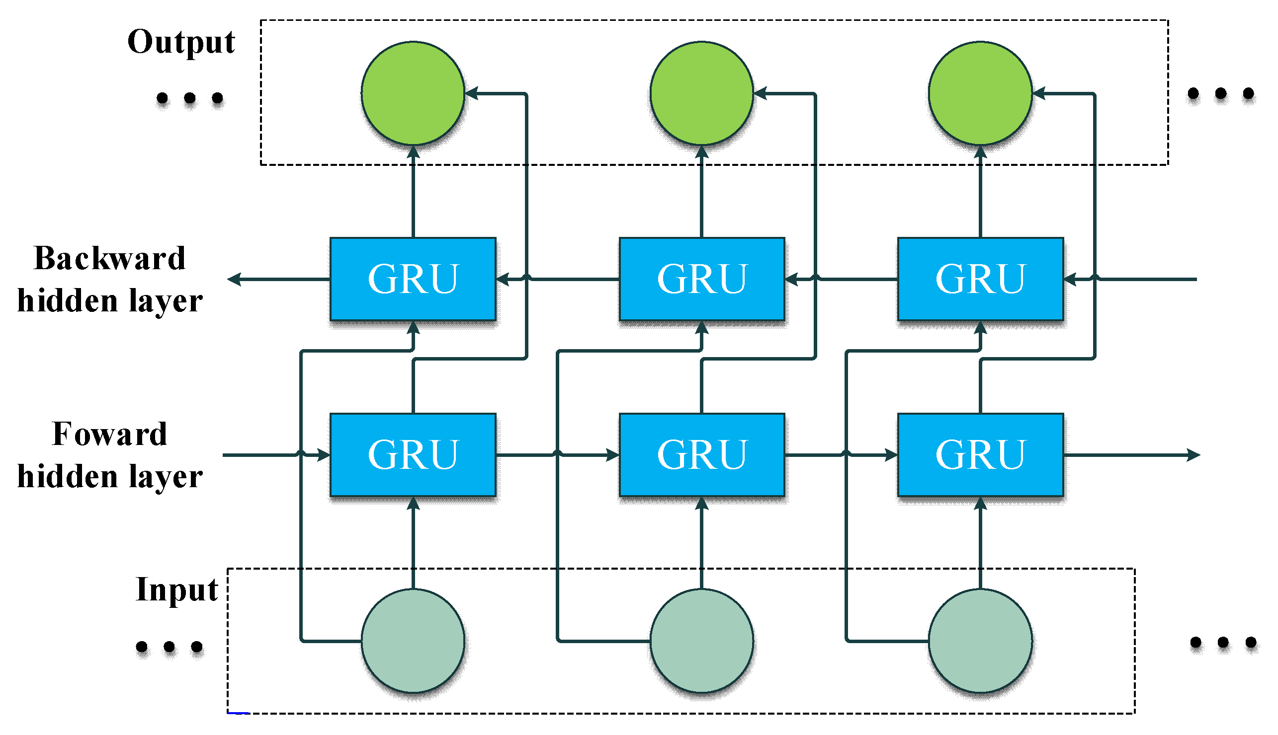
Bi-directional GRU (Bi-GRU) combines two one-way GRU models, one reading the input sequence from the front and the other from the back. By considering both past and future contextual information, Bi-GRU models are better able to capture dependencies and semantic information in sequences [39].

When using Bi-GRU for sequential modeling, the input sequence is first processed through a forward GRU model, and the hidden state of each time step is recorded. Then, the input sequence is processed through a reverse GRU model, and the hidden state of the reverse time step is recorded. Finally, the hidden states of the two models are combined to form a representation of the entire sequence.

By using Bi-GRU, models can take full advantage of past and future context information to extract richer feature representations, thereby improving the performance of sequence modeling tasks. The model structure is shown in Figure 4.

A layer of GRU is added to the basic GRU model, and the two-layer network works simultaneously to obtain both forward and backward feature information, which is able to capture the influence of input information from the past and future on the current state. The horizontal forward GRU hidden layer vector ${\overrightarrow{h}}_t$ and backward GRU hidden layer vector ${\overleftarrow{h}}_t$, are calculated at the same time on each time step t. The signal transmission in the two directions is independent of each other, and the vertical direction represents the unidirectional transmission from the input layer to the hidden layer and then to the output layer. Then the two hidden states are connected to calculate the final result as follows:

$$\begin{array}{c}{\overrightarrow{h}}_t=\mathrm{GRU}\left(x_t,{\overrightarrow{h}}_{t-1}\right)\end{array}$$

(6)

$$\begin{array}{c}{\overleftarrow{\mathrm{h}}}_{\mathrm{t}}=\mathrm{GRU}\left(x_t{,\overleftarrow{\mathrm{h}}}_{\mathrm{t}-1}\right)\end{array}$$

(7)

$$\begin{array}{c}{y}_t=W_t{\overrightarrow{h}}_t+V_t{\overleftarrow{h}}_t+b_y\end{array}$$

(8)

In the formula, GRU (x) represents the GRU function, $W_t$ and $V_t$ are the weights of the forward GRU and the backward GRU, respectively, b_y is the biased representation of the output layer. Bidirectional GRUs can process data features from forward 1→T training and the same data features from reverse T→1 training to better understand time series data features from two different directions, providing an additional environment for neural networks to even fully learn prediction problems.

3.3. Temporal Attention Mechanism (TA)

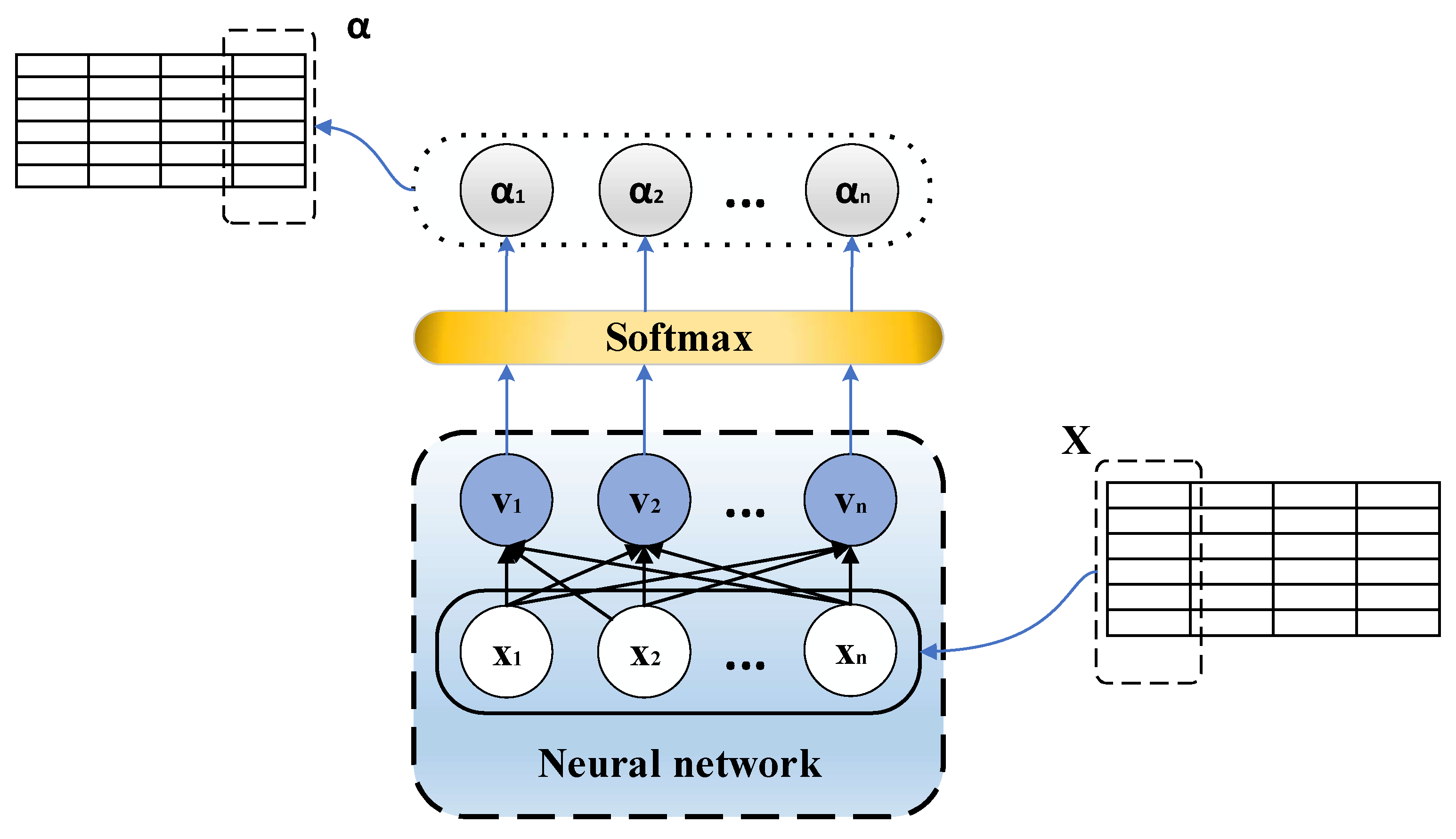
TA (temporal attention) is an mechanism used in sequence modeling that takes into account position information when calculating attention weights [40]. It is commonly utilized for natural language processing (NLP) tasks like machine translation and text summarization. Traditional attention mechanisms compute attention weights by comparing the query vector, typically derived from the hidden state at the previous time step, with each element in the sequence. In contrast, TA not only computes similarity but also considers location information specific to the current time step. The structure of TA’s attention mechanism is depicted in Figure 5.

As shown in the figure above, TA’s attention mechanism has three main stages.

(1)

First, the similarity of the query vector (usually the hidden state from the previous time step, denoted Q) to each element in the sequence is calculated by the formula:

$$\begin{array}{c}\mathrm{similarity}=F(X)\end{array}$$

(9)

(2)

The similarity is normalized to obtain the attention weight (denoted as α). The calculation formula of attention weight is as follows:

$${\alpha }_i\mathrm{softmax}\left(\mathrm{similarity}\right)$$

(10)

The softmax (similarity) function is used to normalize the similarity such that the sum of the attention weights is 1.

(3)

Finally, the attention weight is weighted and summed with each element in the sequence to obtain the output of the attention mechanism. The formula for calculating attention output is:

$$\begin{array}{c}\mathrm{AttentionX}, \mathrm{Source}={\displaystyle \sum _{\mathrm{i}=1}^{{\mathrm{L}}_{\mathrm{x}}}}{\mathsf{\alpha }}_{\mathrm{i}}{*\mathrm{Value}}_{\mathrm{i}}\end{array}$$

(11)

where V represents the value of each element in the sequence, and * represents multiplication at the element level. Through the above calculation formula, TA mechanism considers the similarity between the query vector and each element in the sequence and the similarity of the query vector, and obtains the attention weight of the current time step, and then carries out weighted summations of the sequence to obtain the final output of the attention mechanism.

From the perspective of TA’s functional characteristics, it can effectively focus on the time steps that play a decisive role in prediction in water quality time series data through weighted position information and key feature screening, reducing the interference of irrelevant noise on the model. However, when TA is used alone, it can only allocate weights based on local sequence information and is unable to mine the long-term contextual associations of water quality parameters from both the forward and reverse dimensions as described in Bi-GRU in Section 3.2. The functional shortcomings of the two complement each other precisely—when constructing the TA-Bi-GRU model subsequently, comprehensive bidirectional temporal features can be obtained by relying on Bi-GRU, providing a more complete feature basis for TA. Meanwhile, by enhancing the model’s attention to key water quality change nodes through TA, it compensates for the deficiency of Bi-GRU in focusing on key information, thereby better adapting to the characteristics of nonlinearity and strong temporal correlation of water quality data and providing support for improving prediction accuracy.

3.4. Temporal Attentive Bidirectional Gated Recurrent Unit (TA-Bi-GRU)

TA-Bi-GRU (Temporal Attentive Bidirectional Gated Recurrent Unit) is a time series modeling-oriented deep learning model that integrates two core components: the Bidirectional Gated Recurrent Unit (Bi-GRU, detailed in Section 3.2) and the temporal attention mechanism (TA, detailed in Section 3.3).

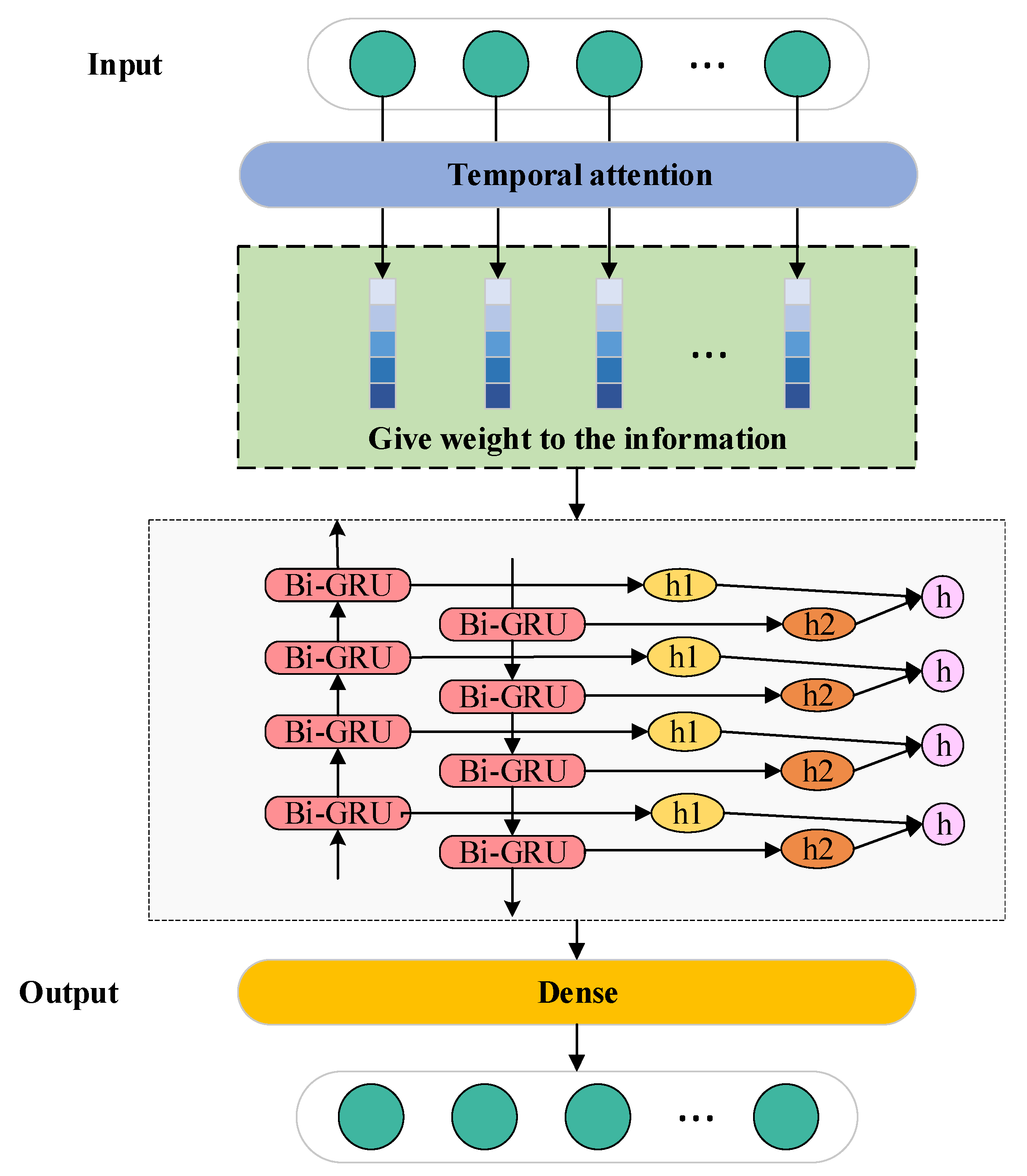
As elaborated in Section 3.2, Bi-GRU’s core advantage lies in its ability to capture bidirectional context dependencies of time series via forward and backward GRUs. TA-Bi-GRU builds on this foundation—instead of redefining Bi-GRU’s structural details, it directly leverages Bi-GRU to extract comprehensive temporal features of water quality data. On this basis, the TA mechanism is introduced to optimize feature selection: it takes the hidden state output by Bi-GRU at each time step as the query vector, calculates attention weights for different time steps, and adaptively enhances the contribution of key temporal information while suppressing irrelevant noise. Finally, the weighted features from the TA mechanism are fused to generate the model’s final output. This integration retains Bi-GRU’s strength in long-term bidirectional dependency capture and complements it with TA’s ability to focus on critical time steps, effectively addressing the limitation of single Bi-GRU in ignoring important temporal details. The structure of the TA-Bi-GRU prediction model is shown in Figure 6.

In addition, to adapt to the characteristics of the water quality data of Xiduan Village Reservoir, which are “limited sample size and strong heterogeneity of index fluctuations”, the structural design parameters of TA-Bi-GRU are centered around “avoiding overfitting and strengthening the capture of key features”: Its Bi-GRU module adopts a 2-layer stacked structure (1 layer of forward GRU+1 layer of reverse GRU). This number of layers can fully explore the bidirectional dependence relationship between short-term fluctuations such as DOX daily dicircadian variation and long-term trends such as TN quarterly accumulation in water quality data, without the need to add additional layers. It can also avoid the overfitting problem and the decline in computational efficiency caused by the sharp increase in model parameter scale when increasing to three layers or more, and is suitable for the training requirements of small and medium-sized water quality datasets. The activation functions are selected based on the characteristics of the functional modules. Among them, the ReLU activation function is selected for the Bi-GRU layer. By taking advantage of its sparse activation characteristics, the vanishing gradient problem of the deep network is alleviated, and at the same time, the sensitivity of the model to cross-time step correlations such as the temporal coupling of pH fluctuations and NH₃N input is enhanced. The Time Distributed layer used for feature dimension matching selects the Tanh activation function and uses its output range of [−1, 1] to compress the water quality data normalized to [0, 1] into the symmetric interval. Effectively alleviate the characteristic transfer shift caused by extreme fluctuations such as the sudden increase of NH₃N from 0.1 mg/L to 0.55 mg/L during the rainy season.

3.5. Prediction Steps for TA-Bi-GRU

The prediction steps of TA-Bi-GRU can be summarized as follows:

(1) In the data preprocessing and input format adaptation stage, the water quality data of Xiduancun Reservoir after preprocessing needs to be reshaped in the format of time step (T) × feature number (F), and the training set (and test set) are divided and compressed to the [0, 1] interval through Min-Max normalization. This operation can avoid the interference of index magnitude differences in the attention weight distribution of TA. Lay the foundation for the collaborative work between TA and Bi-GRU.

(2) The bidirectional temporal feature extraction stage of Bi-GRU is the feature source for TA implementation. Formatted data needs to be input into the two-layer stacked Bi-GRU: the forward GRU traverses the input data in chronological order (t = 1→T), and outputs the forward hidden state sequence ${\overrightarrow{h}}_t$ to focus on the “historical temporal correlation”. The reverse GRU traverses the input data in reverse chronological order (t = T→1) and outputs the reverse hidden state sequence ${\overleftarrow{h}}_t$ to focus on future time series associations. Subsequently, for each time step t, ${\overrightarrow{h}}_t$ and ${\overleftarrow{h}}_t$ are concatenated according to the feature dimension to form the feature output matrix a $H={[h_1^{\text{Bi-GRU}},h_2^{\text{Bi-GRU}},\dots ,h_T^{\text{Bi-GRU}}]}^T\in {ℝ}^{T\times 64}$ of Bi-GRU. This matrix is the core input of the TA mechanism (Query, Key, and Value all come from here), ensuring that TA allocates weights based on the bidirectional temporal features extracted by Bi-GRU. Rather than the original data independent of Bi-GRU.

(3) The specific implementation of TA within the Bi-GRU framework is the core link. It needs to take the hidden state matrix H of Bi-GRU as input and advance according to the logic of “similarity calculation → weight normalization → weighted feature fusion”: For each prediction time step t, taking the Bi-GRU hidden state ${h_t}^{\mathit{\text{Bi-GRU}}}$ of the current time step as the Query (query vector), and the hidden state matrix H of the full time step as the Key (key vector) and Value (value vector), the similarity is calculated using the dot product formula $S_{t\hspace{1em}}=Q\cdot K^T/\sqrt{d}\hspace{1em}={h_t}^{\mathit{\text{Bi-GRU}}}\hspace{1em}\cdot H^T/64$ ($\sqrt{d}$ is the scaling factor). To avoid the disappearance of softmax gradients due to overly large dot product results in high dimensions, the key time steps are initially identified. Then, the similarity vector $S_t$ is normalized by softmax, and the attention weights in the 0–1 interval are obtained through ${\alpha }_t=Softmax(S_t)={\displaystyle \frac{exp(s_{ti})}{{\displaystyle {\sum }_{\mathrm{k}=1}^{T}exp(s_{tk})}}}\hspace{1em}$. High weights (${\alpha }_{ti}=0.82$) are assigned to the time step of the accumulation stage, and low weights (${\alpha }_{tj}=0.04$) are assigned to the time step of the noise stage. At the same time, ${\alpha }_{\min }=0.05$ is set to filter the noise. Finally, the weights ${\alpha }_t$ are weighted and summed with the Value vector H, and the fusion features are output through ($h_t^{\text{TA-Bi-GRU}}={\alpha }_t\cdot V={\displaystyle \sum _{i=1}^T{\alpha }_{ti}}\cdot h_i^{\text{Bi-GRU}}$). Moreover, at the time step of the critical water quality state, the update step size of the TA weights is magnified by 1.2 times to accelerate the model’s learning of the risk of exceeding the standard.

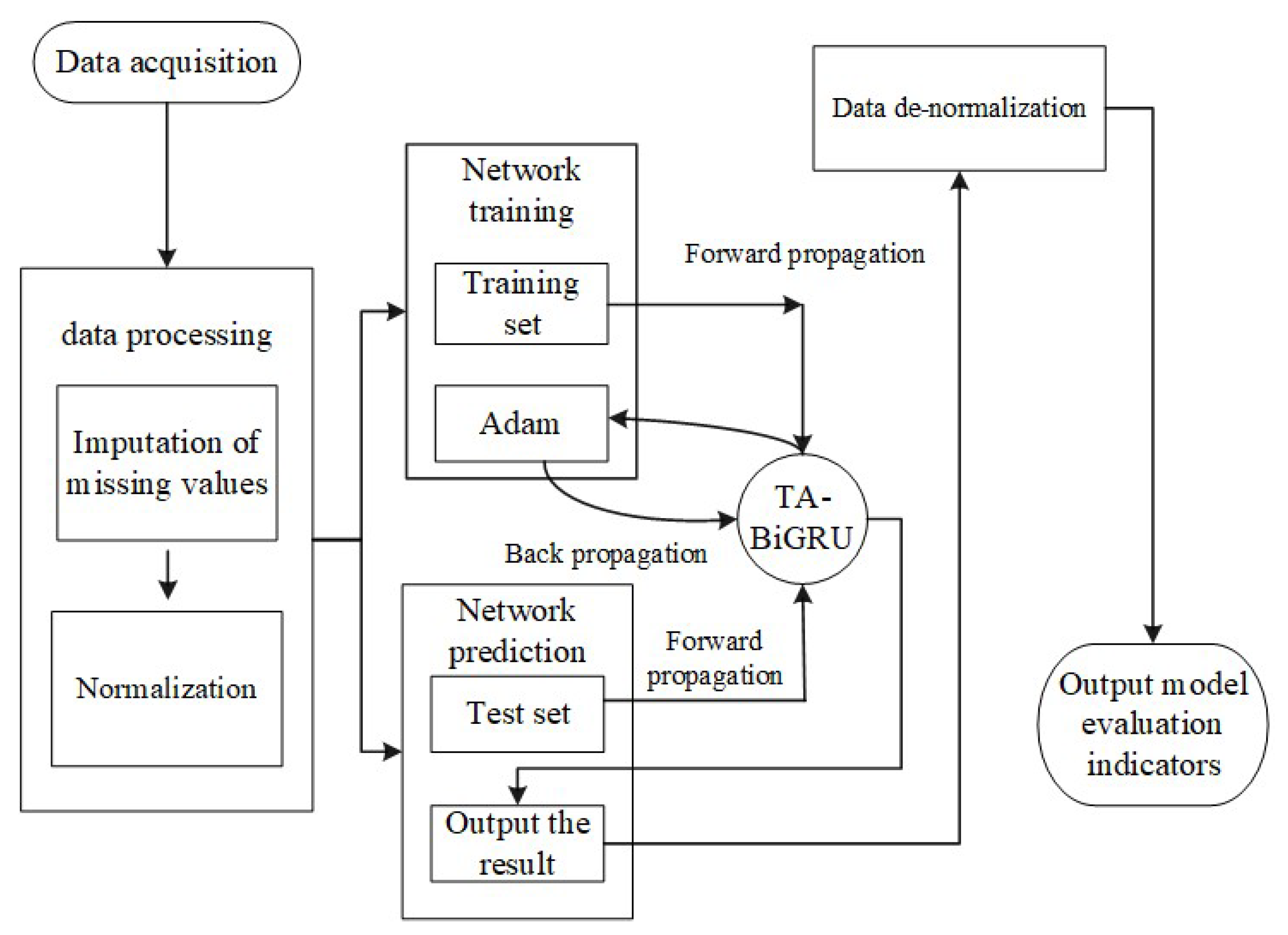
(4) In the model training and prediction output stage, the ${h_t}^{\mathit{\text{TA-Bi-GRU}}}$ feature matrices of all time steps need to be input into the fully connected layer. With MSE as the loss function and Adam as the optimizer, the model weights and bias are optimized using the training set. After the training is completed, the test set data is processed according to the above Bi-GRU feature extraction steps to TA implementation, and the predicted values of DOX, pH, NH₃N, and TN are output. Finally, the data is restored to the original data scale through reverse normalization and compared with the real values to calculate the evaluation indicators such as MAE, MSE, and R². The process of TA-Bi-GRU prediction model is shown in Figure 7.

4. Case Verification

In this paper, four variables including oxygen content (DOX), pH, ammonia nitrogen (NH₃N) and total nitrogen (TN) of water quality data were selected to train GRU, Bi-GRU, TA-GRU, CNN-LSTM, and DeepTCN-LSTM, respectively, and then the test set was predicted to obtain evaluation indicators of each model, so as to compare the superiority of the model.

4.1. Evaluation Index

In this paper, the mean absolute error (MAE), mean square error (MSE) and decision coefficient (R²) are cited as three evaluation indexes. The prediction error of each time series prediction model on the test set can be fully evaluated.

MAE refers to the average distance between the predicted value ${\widehat{y}}_i$ and the true value $y_i$ of the samples. MAE can accurately reflect the true error of the predicted value. From the perspective of the practical significance of water quality prediction, the smaller the MAE value, the smaller the overall prediction deviation of the model for water quality indicators, which can more accurately reflect the daily fluctuations of water quality. A smaller MAE can narrow the absolute error range between the predicted value and the true value, reduce the probability of misjudgment of water quality exceeding standards, and provide a more reliable basis. The calculation formula of MAE is shown in Equation (12).

$$\begin{array}{c}\mathrm{MAE}={\displaystyle \frac{1}{\mathrm{m}}}{\displaystyle \sum _{\mathrm{i}=1}^{\mathrm{m}}}\left|{\mathrm{y}}_{\mathrm{i}}{-\widehat{\mathrm{y}}}_{\mathrm{i}}\right|\end{array}$$

(12)

In the above formula, m represents the number of samples in the test set, $y_i$ and ${\widehat{y}}_i$ represent the true value and predicted value of the i-th sample, respectively,

MSE refers to the expected value of the square of the difference between the estimated value and the true value of the parameter, which can be used to evaluate the degree of data variation. From the practical significance of water quality prediction, MSE amplifies the weight of larger deviations by squaring the deviations, and thus is more sensitive to extreme water quality changes. The smaller the MSE value is, the higher the prediction accuracy of the model for such key extreme value changes is. If the MSE value is large, it indicates that there are many prediction results with significant deviations, which may misjudge abnormal water quality conditions and thereby affect the scientific nature of water quality governance decisions. The MSE calculation is as shown in Equation (13).

$$\begin{array}{c}\mathrm{MSE}={\displaystyle \frac{1}{\mathrm{m}}}{\displaystyle \sum _{\mathrm{i}=1}^{\mathrm{m}}}{\left({\mathrm{y}}_{\mathrm{i}}{-\widehat{\mathrm{y}}}_{\mathrm{i}}\right)}^2\end{array}$$

(13)

R-squared (R²) represents the goodness of fit of the model, with a value range of [0, 1]. The closer it is to 1, the better the consistency between the predicted value and the actual value.

$$\begin{array}{c}{R}^2=1-{\displaystyle \frac{{{\displaystyle \sum }}_{j=1}^{n_d}{\left(y_{observed}\left(j\right)-y_{pred}\left(j\right)\right)}^2}{{\displaystyle {\sum }_{j=1}^{n_d}}{\left(y_{observed}\left(j\right)-\overline{y}\right)}^2}}\end{array}$$

(14)

In the formula, $y_{observed}$ is the actual measured value corresponding to the test sample; $y_{pred}$ is the predicted value; $\overline{y}$ is the sample mean calculated according to the actual measured value of the sample; $n_d$ is the number of test samples.

4.2. Model Parameters and Experimental Environment

This section focuses on the core hyperparameter Settings, selection basis, and system adjustment process. All hyperparameters are tested and optimized within the preset range through the “control variable method” to ensure they meet the requirements of water quality prediction tasks. All hyperparameters are optimized through “single-variable control + cross-validation” First, fix the basic parameters, test a single hyperparameter within the preset range, and record the test set MSE and R² of the model under different values. After a single hyperparameter is determined, fix that parameter and optimize the next one. Eventually, the combination of “stable training convergence and optimal test generalization” is screened out. For instance, the cross-test of the learning rate and batch size shows that when the learning rate is 0.001 and the batch size is 32, the model converges within 100 epochs and has the highest prediction accuracy. Therefore, this combination is determined. The specific parameters and explanations are shown in

Table 3. Hyperparameters of four prediction models.

Model	Argument	Selection Basis and System Adjustment Process
Time Distributed activation (inputs)	Tanh	It is more stable than Sigmoid, ADAPTS to the feature transmission of water quality data, and alleviates the impact of extreme value fluctuations.
Time Distributed activation (attention)	Softmax	The standard normalization method of the temporal attention mechanism ensures that the sum of the attention weights is 1.
Weighted_inputs axis	2	Match the characteristic dimensions of four core water quality indicators.
Weighted_sum axis	1	Align the time step dimension and test that the temporal correlation breaks when axis = 0, so set it to 1.
Bi-GRU layer activation function	ReLU	It can alleviate gradient vanishing better than Sigmoid and Leaky ReLU and improve the capture accuracy of key temporal correlation.
Optimizer	Adam	Compared with SGD and RMSprop, it achieves a better balance between convergence speed and stability, adapting to the heterogeneity of exponential fluctuations.
Loss function	MSE	Amplifying the errors related to water quality safety is more in line with the early warning requirements of water sources than MAE.
Learning rate	0.001	[0.01, 0.001, 0.0001] In the test, 0.001 has the best generalization.
batch_size	32	[16, 32, 64] In the test, 32 training stability and data diversity.
Epoch	100	In the tests of [100, 200, 300], the training loss for 100 years was stable and there was no overfitting.
Weight attenuation	1 × 10−5	In the [1 × 10−4, 1 × 10−5, 1 × 10−6] tests, 1 × 10−5 can optimally increase R2 by 0.02 to 0.03.

.

4.3. Training Loss

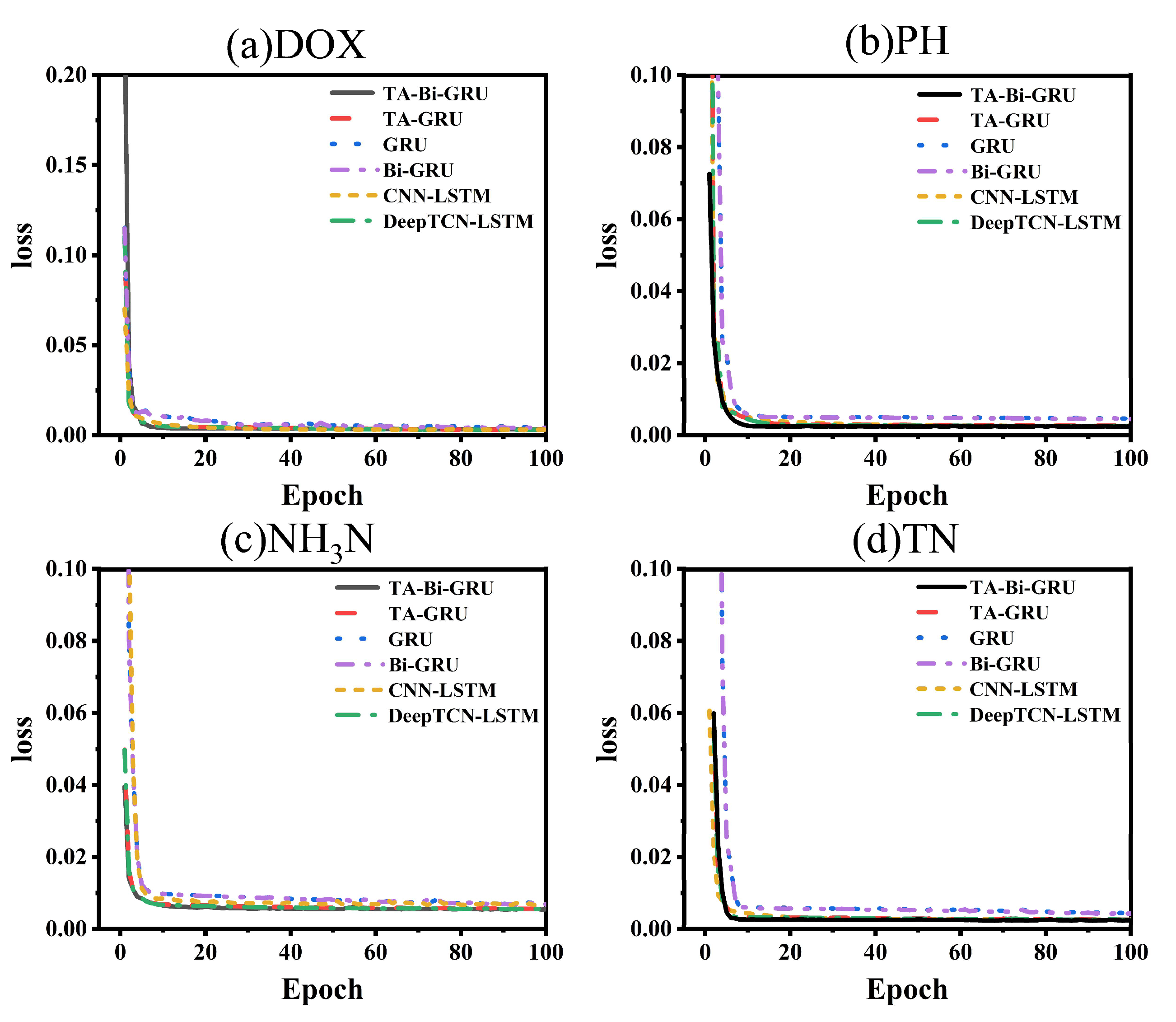
With the advancement of training iterations, the training losses of the six types of models, namely GRU, Bi-GRU, TA-GRU, CNN-LSTM, DeepTDN-LSTM and TA-Bi-GRU, for the four indicators of DOX, pH, NH₃N and TN have gradually decreased and stabilized. Overall, it follows the pattern of rapid decline in the early stage and gentle stability in the later stage. Figure 8 clearly presents the differences among various models. Moreover, TA-Bi-GRU always maintains the fastest convergence and the lowest final loss. Although CNN-LSTM and DeepTDN-LSTM are superior to the traditional basic models, they are not as good as TA-Bi-GRU.

In terms of convergence speed, the performance of different models in the four types of indicators is consistent, and the characteristics of the indicators have a significant impact on the convergence efficiency. The pH index has the smallest daily fluctuation range, and the overall convergence speed of each model is the fastest. The TA-Bi-GRU is stable in the first 10 iterations. CNN-LSTM and DeepTDN-LSTM require 15–18 iterations, and TA-GRU requires 12 iterations. The basic models Bi-GRU and GRU require 20 and 25 times, respectively. In DOX, TA-Bi-GRU is stable for the first 20 times. Deeptdn-lstm and CNN-LSTM require 28 and 30 times, respectively, TA-GRU requires 35 times, and the basic model GRU and Bi-GRU require 50 and 40 times, respectively. In NH₃N and TN (long-term accumulation), TA-Bi-GRU is stable for the first 20–25 times, DeepTCN-LSTM and CNN-LSTM require 28–35 times, TA-GRU requires 35–40 times, and the basic model requires 45–60 times. From the perspective of the final loss of iteration, the TA-Bi-GRU has the lowest full indicators (DOX 0.0031, pH 0.0024, NH₃N 0.0068, TN 0.0027); The losses of the basic models were significantly higher (such as GRU DOX 0.0062, pH 0.0056, NH₃N 0.0094, TN 0.0046), while Bi-GRU was slightly lower than GRU (DOX 0.0053, pH 0.0042, NH₃N 0.0094, TN 0.0046). TA-GRU, due to the integration of the attention mechanism, has improved losses compared to the basic model (DOX 0.0043, pH 0.0036, NH₃N 0.0077, TN 0.0035). CNN-LSTM and DeepTCN-LSTM each have adaptation advantages but limitations: CNN-LSTM is good at capturing short-term local fluctuations. Its DOX loss is 0.0039 and pH is 0.0028. However, the unidirectional cyclic structure cannot utilize future time series information, resulting in higher losses of NH₃N (0.0085) and TN (0.0038). Deeptdn-lstm has better adaptability to long-period indicators with dilated convolution, with NH₃N loss of 0.0081 and TN loss of 0.0035. However, fixed convolution kernels are difficult to adapt to nonlinear fluctuations, and the losses of DOX (0.0042) and pH (0.0030) are slightly higher than those of CNN-LSTM. The final loss of TA-Bi-GRU is at the lowest level among the four types of indicators: DOX is 0.0031, pH is 0.0024, NH₃N is 0.0068, and TN is 0.0027. The experimental results show that TA-Bi-GRU, through the synergy of Bi-GRU and TA mechanisms, solves the problems of slow convergence and high loss of the basic model and breaks through the limitations of the combined model. Verify the adaptability and rationality of its structure to the time series data of water quality.

4.4. Analysis of Experimental Results

4.4.1. Performance Verification and Analysis of the Model

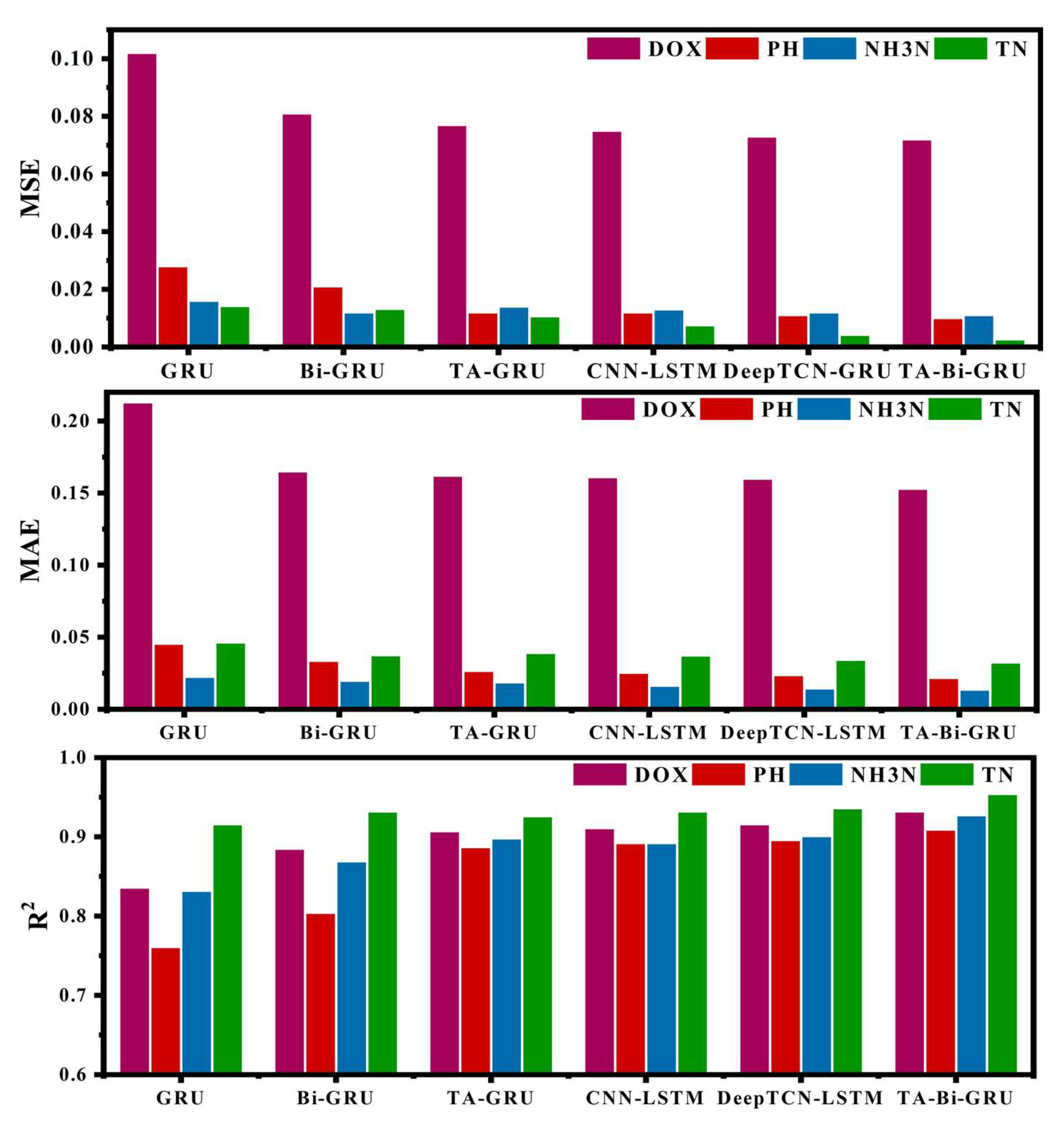
To assess the predictive superiority of the TA-Bi-GRU model, predictions were made for pH, ammonia nitrogen (NH₃N), total nitrogen (TN), and dissolved oxygen (DOX). The predicted results were then compared and analyzed against those of the other models.

Table 4. Model evaluation index.

	Model	MSE	MAE	R2
DOX	GRU	0.102	0.213	0.836
	Bi-GRU	0.081	0.165	0.885
	TA-GRU	0.077	0.162	0.907
	CNN-LSTM	0.075	0.161	0.911
	DeepTCN-LSTM	0.073	0.160	0.916
	TA-Bi-GRU	0.072	0.159	0.932
pH	GRU	0.028	0.0454	0.761
	Bi-GRU	0.021	0.0336	0.804
	TA-GRU	0.012	0.0266	0.887
	CNN-LSTM	0.012	0.0253	0.892
	DeepTCN-LSTM	0.011	0.0237	0.896
	TA-Bi-GRU	0.010	0.0217	0.909
NH3N	GRU	0.016	0.0104	0.882
	Bi-GRU	0.012	0.0082	0.899
	TA-GRU	0.014	0.0102	0.908
	CNN-LSTM	0.013	0.0093	0.902
	DeepTCN-LSTM	0.012	0.0082	0.901
	TA-Bi-GRU	0.011	0.0072	0.917
TN	GRU	0.0142	0.0463	0.916
	Bi-GRU	0.0132	0.0375	0.932
	TA-GRU	0.0106	0.0391	0.926
	CNN-LSTM	0.0075	0.0372	0.932
	DeepTCN-LSTM	0.0042	0.0343	0.936
	TA-Bi-GRU	0.0026	0.0325	0.964

presents the evaluation and comparison results using the MSE, MAE, and R² statistical indicators. Figure 9 provides a more intuitive representation of the indicators for the four models.

Table 4 presents the evaluation results of the prediction performance of six types of models, namely GRU, Bi-GRU, TA-GRU, TA-Bi-GRU, and the newly added CNN-LSTM and DeepTDN-GRU, on the four core water quality indicators of DOX, pH, NH₃N, and TN. From the perspective of the overall model, TA-Bi-GRU still performs the best in the prediction of all water quality indicators and consistently shows a stable trend of performance improvement. Compared with the GRU model used as the baseline, the MAE of TA-Bi-GRU decreased by 15–35% in each indicator, the MSE decreased by 25–45%, and the R² increased by 8–12%. Even compared with TA-GRU, which integrates unidirectional GRU and TA mechanisms, and Bi-GRU, which has bidirectional timing capture capabilities, the advantages of TA-Bi-GRU remain significant. Its MAE is 5–15% lower than that of TA-GRU and 10–20% lower than that of Bi-GRU MSE decreased by 8–20% compared with TA-GRU and by 12–25% compared with Bi-GRU, while R² increased by 1–3% and 2–5%, respectively, compared with the two. The newly added CNN-LSTM and DeepTDN-GRU have overall performance that lies between TA-GRU/Bi-GRU and TA-Bi-GRU. CNN-LSTM, with its ability to extract local time series features of water quality data through convolutional layers, reduces MAE in DOX and pH indicators by 24–31% compared to GRU, reduces MSE by 26–33%, and increases R² by 8–10% compared to GRU. Slightly better than Bi-GRU but slightly inferior to TA-GRU; Deeptdn-gru enhances the ability to capture long sequence dependencies by leveraging the dilation characteristics of temporal convolution kernels. It has better adaptability to indicators with long-period cumulative features such as NH₃N and TN. For instance, the MSE of the TN indicator drops to 0.0042 and the R² reaches 0.936, with performance approaching that of TA-GRU. But still not as good as TA-Bi-GRU.

Further observation of the specificity of the indicators reveals that the improvement of TA-Bi-GRU in TN and DOX indicators is particularly prominent, and this advantage is even more evident when compared with the newly added models: TN, as a key indicator reflecting eutrophication of water bodies, its R² reached 0.964 in the TA-Bi-GRU model, which was nearly 5 percentage points higher than that of GRU and 3.4 percentage points higher than that of CNN-LSTM (0.932). It was 2.8 percentage points higher than DeepTCN-LSTM (0.936); DOX, as a core parameter characterizing the self-purification capacity of water bodies, the MAE predicted by TA-Bi-GRU decreased to 0.159, which was 1.2% and 0.6% lower than that of CNN-LSTM (0.161) and DeepTDN-GRU (0.160), respectively. MSE decreased by 4.0% and 1.4%, respectively, compared with the two. Although the decrease was not significant, combined with R², it can be known that TA-Bi-GRU has better fitting stability for the long-term fluctuation trend of DOX. The core reason for this difference lies in: The unidirectional cyclic structure of CNN-LSTM cannot utilize future temporal information to correct the current prediction bias. The fixed convolution kernel of DeepTCN-LSTM is difficult to dynamically adapt to the nonlinear mutation characteristics of water quality indicators, while TA-Bi-GRU captures bidirectional temporal correlations through Bi-GRU. At the same time, with the help of the TA mechanism, key time step information is precisely screened. The two work together to make up for the deficiencies of the single-structure model in feature extraction and information focus. Even when compared with the newly added high-performance hybrid model, it can still achieve better prediction accuracy and stability.

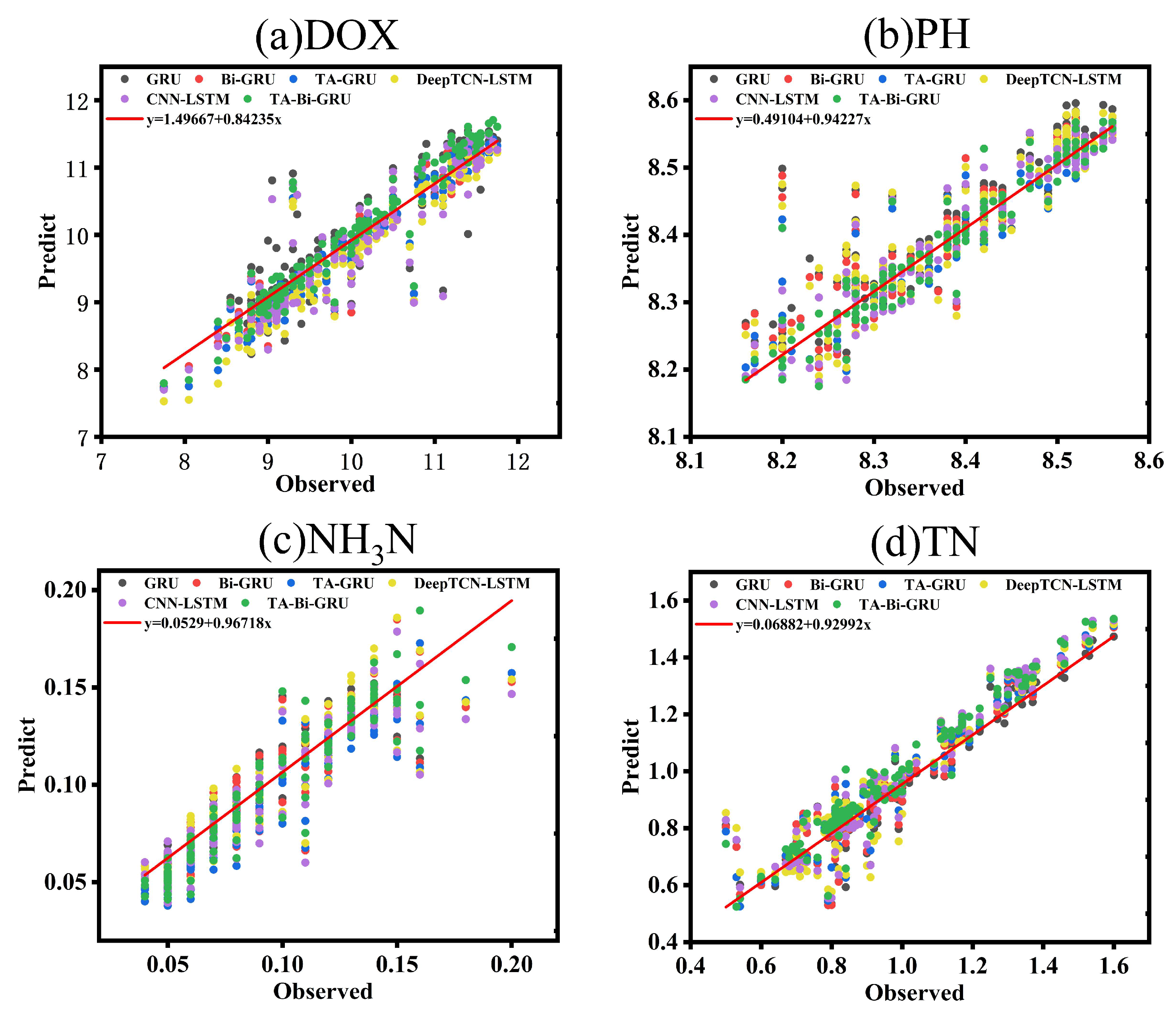
Figure 10 presents the scatter plots and linear fitting of pH, ammonia nitrogen (NH₃N), total nitrogen (TN), and dissolved oxygen (DOX) predicted by six different prediction models. Compared with the GRU model, Bi-GRU model, TA-GRU, CNN-LSTM and DeepTCN-LSTM models, the linear fitting result of the TA-Bi-GRU model is closer to the true value. This observation further supports the superior predictive performance of the TA-Bi-GRU model.

4.4.2. Experiment on the Influence of Training Set Size on Model Performance

To verify the robustness of the TA-Bi-GRU model in the scenario of small sample data, this experiment keeps the total sample size (785 day-scale samples) unchanged. By adjusting the division ratio of the training set and the test set (30%/70%, 50%/50%, 70%/30%, compared with 80%/20% in the original experiment), Analyze the performance variation patterns of each model under different training data volumes. In the experiment, keep the model hyperparameters (learning rate 0.001, batch_size = 32, epoch = 100) and evaluation indicators (MAE, MSE, R²) unchanged, and focus on the average values of the four core indicators: DOX, pH, NH₃N, and TN. The results are shown in

Table 5. The average predictive performance of each model under different training set scales.

Training Set Ratio	Model	Average MAE	Average MSE	Average R2
30%	GRU	0.122	0.108	0.515
	Bi-GRU	0.107	0.088	0.583
	TA-GRU	0.102	0.083	0.613
	CNN-LSTM	0.100	0.082	0.622
	DeepTCN-LSTM	0.096	0.079	0.645
	TA-Bi-GRU	0.087	0.073	0.692
50%	GRU	0.104	0.087	0.605
	Bi-GRU	0.085	0.069	0.672
	TA-GRU	0.080	0.065	0.704
	CNN-LSTM	0.079	0.064	0.714
	DeepTCN-LSTM	0.076	0.061	0.731
	TA-Bi-GRU	0.073	0.058	0.775
70%	GRU	0.086	0.073	0.685
	Bi-GRU	0.074	0.056	0.751
	TA-GRU	0.068	0.051	0.785
	CNN-LSTM	0.066	0.050	0.794
	DeepTCN-LSTM	0.063	0.048	0.810
	TA-Bi-GRU	0.058	0.044	0.839

.

The performance of all comparison models showed a significant optimization trend as the proportion of the training set increased. Taking TA-Bi-GRU as an example, when the training set increased from 30% to 80%, the average R² increased from 0.692 to 0.930, and the average MAE decreased from 0.087 to 0.055. The average MSE decreased from 0.073 to 0.049, indicating that more training data can provide the model with more sufficient temporal feature learning samples, reduce overfitting of limited samples, and thereby enhance the generalization ability. Compared with other models, TA-Bi-GRU has a smaller performance degradation when the proportion of the training set decreases. For example, in the scenario of a 30% training set, its average R² is 0.692. It was 34.4%, 18.7% and 11.2% higher than GRU (0.515), Bi-GRU (0.583) and CNN-LSTM (0.622), respectively, and the average MAE was 26.3% lower than that of GRU (0.122). This stems from its “bidirectional temporal perception + dynamic attention” structure—Bi-GRU can maximize the mining of “history-future” correlations by bidirectionally traversing limited data. The TA mechanism can focus on key time steps to reduce non-critical noise interference, enabling the model to efficiently extract core features even when the data volume is insufficient. Meanwhile, there is a nonlinear relationship between the model performance and the size of the training set. The performance improvement is the greatest when the training set increases from 30% to 50% (the average R² of TA-Bi-GRU increases by 0.083), and the improvement slows down when it increases from 70% to 80% (the average R² increases by 0.045), reflecting the “marginal effect”. That is, when the data volume reaches a certain threshold, simply increasing the data will reduce the performance gain. At this time, the model performance is more affected by the rationality of the structure. Based on the above rules, it can be inferred that when the scale of the training set is further expanded (such as increasing to 90% of the training set or introducing 1825 day-scale samples over 5 years), the overall performance of the model will continue to improve but the growth rate will slow down. Referring to the change from “70% to 80% of the training set”, When the training set increases to 90%, the average R² of TA-Bi-GRU can be raised to 0.94–0.95, and the MAE and MSE can be further reduced by 5–8%. When the data is increased to 5 years, more cross-year climate anomaly scenarios can be learned, and the average R² is expected to exceed 0.96. Moreover, the leading advantage of TA-Bi-GRU will be further consolidated. Its “bidirectional + attention” structure can more accurately capture the long-tail features in the newly added data, while other models have relatively low learning efficiency for such rare features. The leading advantage will be stably maintained at 10–15%, and its small sample robustness can be extended to cross-basin data adaptation. Even if the data volume of the new river basin is relatively small, it can be quickly adapted through “trained multi-river basin features + focus on key time steps of the new river basin”, providing support for cross-regional water quality prediction. In summary, TA-Bi-GRU performs well in both scenarios with sufficient data and small samples, and its performance is continuously optimized as the dataset expands, providing a basis for practical promotion.

4.4.3. Performance Verification and Analysis of the Model Under Multiple Prediction Periods

The prediction period for the above-mentioned experiment is one day. The performance of the TA-Bi-GRU prediction model is superior to that of other models. To investigate the performance of the TA-Bi-GRU model in different prediction periods, we used the same model parameters and selected 7 days, 10 days, 15 days and 30 days respectively as the prediction periods of the model for prediction. The comparison of various evaluation indicators obtained from the experiment is shown in

Table 6. Evaluation metrics for different prediction horizons.

Forecast Horizon	Index	Model	MSE	MAE	R2
7 d	DOX	GRU	0.185	0.302	0.768
		Bi-GRU	0.142	0.248	0.812
		TA-GRU	0.131	0.235	0.835
		CNN-LSTM	0.127	0.231	0.84
		DeepTCN-LSTM	0.122	0.226	0.845
		TA-Bi-GRU	0.115	0.218	0.858
	pH	GRU	0.045	0.0628	0.692
		Bi-GRU	0.036	0.0515	0.736
		TA-GRU	0.021	0.0382	0.816
		CNN-LSTM	0.02	0.0375	0.815
		DeepTCN-LSTM	0.019	0.0368	0.827
		TA-Bi-GRU	0.017	0.0342	0.830
	NH3N	GRU	0.028	0.0215	0.808
		Bi-GRU	0.022	0.0168	0.825
		TA-GRU	0.024	0.0198	0.832
		CNN-LSTM	0.023	0.0189	0.826
		DeepTCN-LSTM	0.022	0.0168	0.825
		TA-Bi-GRU	0.019	0.0151	0.845
	TN	GRU	0.0285	0.0638	0.835
		Bi-GRU	0.0268	0.0598	0.850
		TA-GRU	0.0252	0.0572	0.862
		CNN-LSTM	0.0249	0.0567	0.860
		DeepTCN-LSTM	0.0241	0.0551	0.875
		TA-Bi-GRU	0.0218	0.0502	0.893
10 d	DOX	GRU	0.248	0.365	0.692
		Bi-GRU	0.182	0.302	0.738
		TA-GRU	0.195	0.288	0.763
		CNN-LSTM	0.176	0.282	0.765
		DeepTCN-LSTM	0.17	0.275	0.772
		TA-Bi-GRU	0.158	0.263	0.762
	pH	GRU	0.062	0.0735	0.615
		Bi-GRU	0.052	0.0638	0.658
		TA-GRU	0.032	0.0478	0.725
		CNN-LSTM	0.031	0.047	0.731
		DeepTCN-LSTM	0.03	0.0461	0.735
		TA-Bi-GRU	0.026	0.0435	0.740
	NH3N	GRU	0.038	0.0278	0.725
		Bi-GRU	0.034	0.0258	0.748
		TA-GRU	0.031	0.0244	0.756
		CNN-LSTM	0.032	0.0249	0.745
		DeepTCN-LSTM	0.031	0.0225	0.748
		TA-Bi-GRU	0.027	0.0208	0.783
	TN	GRU	0.0392	0.0765	0.740
		Bi-GRU	0.0378	0.0702	0.755
		TA-GRU	0.0358	0.0731	0.763
		CNN-LSTM	0.0358	0.0702	0.775
		DeepTCN-LSTM	0.0345	0.0681	0.782
		TA-Bi-GRU	0.0305	0.0658	0.804
15 d	DOX	GRU	0.325	0.428	0.605
		Bi-GRU	0.268	0.372	0.652
		TA-GRU	0.251	0.355	0.672
		CNN-LSTM	0.243	0.348	0.678
		DeepTCN-LSTM	0.235	0.34	0.685
		TA-Bi-GRU	0.22	0.328	0.715
	pH	GRU	0.085	0.0862	0.523
		Bi-GRU	0.075	0.0785	0.565
		TA-GRU	0.048	0.0592	0.617
		CNN-LSTM	0.047	0.0583	0.615
		DeepTCN-LSTM	0.046	0.0572	0.622
		TA-Bi-GRU	0.041	0.0548	0.647
	NH3N	GRU	0.052	0.0352	0.620
		Bi-GRU	0.048	0.0338	0.642
		TA-GRU	0.045	0.0305	0.653
		CNN-LSTM	0.046	0.0329	0.659
		DeepTCN-LSTM	0.045	0.0305	0.667
		TA-Bi-GRU	0.039	0.0285	0.693
	TN	GRU	0.0538	0.0926	0.585
		Bi-GRU	0.0502	0.0875	0.592
		TA-GRU	0.0521	0.0902	0.613
		CNN-LSTM	0.0502	0.0875	0.620
		DeepTCN-LSTM	0.0485	0.0848	0.638
		TA-Bi-GRU	0.0458	0.0825	0.680
30 d	DOX	GRU	0.412	0.495	0.482
		Bi-GRU	0.352	0.442	0.525
		TA-GRU	0.331	0.42	0.54
		CNN-LSTM	0.322	0.412	0.545
		DeepTCN-LSTM	0.311	0.401	0.557
		TA-Bi-GRU	0.295	0.385	0.585
	pH	GRU	0.118	0.0985	0.384
		Bi-GRU	0.105	0.0921	0.427
		TA-GRU	0.072	0.0735	0.452
		CNN-LSTM	0.07	0.0723	0.455
		DeepTCN-LSTM	0.068	0.0708	0.465
		TA-Bi-GRU	0.062	0.0682	0.520
	NH3N	GRU	0.07	0.0438	0.494
		Bi-GRU	0.062	0.0395	0.515
		TA-GRU	0.065	0.0418	0.519
		CNN-LSTM	0.064	0.0409	0.525
		DeepTCN-LSTM	0.062	0.0395	0.527
		TA-Bi-GRU	0.055	0.0372	0.545
	TN	GRU	0.0725	0.1128	0.455
		Bi-GRU	0.0682	0.1075	0.462
		TA-GRU	0.0705	0.1102	0.469
		CNN-LSTM	0.0682	0.1075	0.470
		DeepTCN-LSTM	0.0665	0.1048	0.480
		TA-Bi-GRU	0.0638	0.1025	0.550

. Figure 11 more intuitively represents the size and variation of the model evaluation metrics within different prediction ranges.

It can be known from Table 6 and Figure 11 that in the prediction periods of 7 days, 10 days, 15 days and 30 days for the six types of models, namely GRU, Bi-GRU, TA-GRU, CNN-LSTM, DeepTCN-LSTM and TA-Bi-GRU, the longer the prediction period, The common rule is that MSE and MAE increase while R² decreases. However, the performance levels and attenuation rates of each model vary significantly. Specifically, they can be analyzed hierarchically by model type:

The basic models (GRU, Bi-GRU) have the poorest performance and the fastest degradation due to the lack of attention mechanism and bidirectional temporal perception ability: Taking the DOX indicator as an example, the GRU increased from 7 days to 30 days, the MSE rose from 0.185 to 0.412 (an increase of 122.7%), and the R² dropped from 0.768 to 0.482 (a decrease of 37.2%). Although Bi-GRU is slightly better than GRU, the R² of pH at 30 days is only 0.427, a decrease of 42.0% compared with 0.736 at 7 days. It can also be intuitively observed from Figure 11 that the MSE/MAE curves of these two types of models are always at the top, while the R² curve is at the bottom with the largest slope, clearly reflecting that their performance degradation rate is the fastest.

TA-GRU screens key information by means of the temporal attention mechanism and has better performance than the basic model. However, it is limited by the temporal perception defect of unidirectional GRU and still cannot compete with other advanced models in long periods: the R² of NH₃N in 7 days is 0.832, which is 3.0% higher than that of GRU (0.808). However, the R² of this indicator dropped to 0.519 at 30 days, a decrease of 37.6% compared with 7 days, which was significantly greater than 35.5% of TA-Bi-GRU. Moreover, the MSE of TN reached 0.0705 at 30 days. It was higher than DeepTCN-LSTM (0.0665) and TA-Bi-GRU (0.0638).

The combined models (CNN-LSTM, DeepTDN-GRU) each have their own adaptation advantages but also have structural limitations: CNN-LSTM extracts local temporal features by convolutional layers. The MSE of 7-day DOX is 0.127, which is 31.4% lower than that of GRU (0.185). However, unidirectional LSTM cannot utilize future temporal information. The R² of DOX in 30 days decreased from 0.84 to 0.545 (a reduction of 35.1%). Deeptdn-gru ADAPTS long-period indicators (such as TN) through dilated convolution. The MSE of TN in 7 days is 0.0241, which is 3.2% lower than that of CNN-LSTM (0.0249), but the fixed convolution kernel is difficult to adapt to the nonlinear fluctuations of water quality. The R² of NH₃N at 30 days was 0.527, which was lower than that of TA-Bi-GRU (0.545). In Figure 11, the index curves of these two types of models always lie between the basic model and TA-Bi-GRU, gradually approaching the basic model as the period extends, confirming the performance degradation caused by their structural limitations.

The TA-Bi-GRU proposed in this study, relying on the synergistic advantages of Bi-GRU’s bidirectional timing capture and the dynamic focus of key time steps by the TA mechanism, maintains the optimal performance in each period and each indicator, and has the slowest attenuation rate: The MSE of 7-day TN was only 0.0218 (9.5% lower than DeepTDN-GRU), and the R² of 30-day pH reached 0.520 (14.3% higher than CNN-LSTM). From 7 days to 30 days, the average R² decrease was only 32.1%, significantly lower than that of models such as GRU (40.3%) and CNN-LSTM (35.1%). Taking TN as an example, the R² of TA-Bi-GRU decreased from 0.893 to 0.550 (a decrease of 38.4%). It was only 85.1% of the decline in DeepTCN-LSTM (45.1%). In Figure 11, the MSE/MAE curve of the TA-Bi-GRU is always at the bottom, and the R² curve is always at the top with the smallest slope. This fully verifies its adaptability to long-term water quality prediction and can provide reliable technical support for pollution prevention and control in water sources on a quarterly to semi-annual scale.

5. Discussion

The precise prediction of water quality time series data is the core technical support for the active prevention and control of water pollution. Especially for drinking water sources like Xiduan Village Reservoir that undertake the “living-production-ecological” three-life water supply function, their water supply balance is highly dependent on reliable long-term water quality forecasting. The TA-Bi-GRU model proposed in this study not only overcomes the inherent limitations of existing models in environmental time series prediction, but also provides a practical technical solution for actual water resource management. The results have both academic value and engineering significance, but they need to be further developed through comparison with similar studies, analysis of model adaptability, and emphasis on actual application scenarios.

5.1. Significance of the Research Results: Comparison with Similar Studies

The existing deep learning models for water quality prediction often encounter the contradiction between “short-term accuracy” and “long-term stability”. For example, the DeepTCN-GRU water quality prediction model proposed by Tian et al. [41] achieved an R² of 0.93 in the 1-day ph prediction, but when extended to the 11-day prediction, the R² dropped to 0.21, and the accuracy attenuation rate reached 77.4%. Chen et al. [42] used the Attention Bi-LSTM model to predict the water station data of Zhuhai Bridge. When the prediction period was extended from 1 day to 10 days, the mean absolute error (RMSE) of the model increased by 182%. When the prediction period of the above two models increased to 10 days, The reliability of the model’s prediction results can no longer be guaranteed. In contrast, for the TA-Bi-GRU model in this study, the 30-day predicted average coefficient of determination (R²) remained at 0.553 (Table 6), and the decay rate compared to the 7-day benchmark (0.858) was only 32.1%, which was much lower than the decay rates of DeepTDN-GRU and CNN-LSTM from 1 day to 10 days. Fully verify its long-term predictive stability advantage.

From a methodological perspective, traditional bidirectional models and attention-enhanced unidirectional models struggle to balance “temporal integrity” and “focus on key information”. When Sheng et al. [43] conducted predictions using the Bi-GRU model, they found that although bidirectional timing capture improved short-term accuracy, it was unable to prioritize key time steps, resulting in a 10.2% decrease in the 7-day prediction accuracy. Liao et al. [44] used the LSTM-AT model in the prediction of short-term wind speed. Although it could screen out key features, it was limited by one-way temporal perception, and the attenuation rate of MAE from 1 h to 5 h reached 31.73%. And TA-Bi-GRU, through the integration of Bi-GRU and temporal attention (TA), precisely resolves this predicament: Bi-GRU captures bidirectional dependencies (such as the coupling of early rainfall and later NH₃N runoff), and the TA mechanism dynamically assigns high weights to key time steps, enabling it in the 7–30 day full-cycle prediction. All are superior to single-structure models and hybrid models, such as CNN-LSTM and DeepTDN-LSTM (Table 6, Figure 11). This advantage precisely aligns with the core requirements of environmental time series prediction, which not only need to fit historical data but also capture nonlinear, long-period, and event-driven fluctuations, filling the gap between the short-term bias of existing models and the actual long-term management needs.

5.2. The Adaptability of TA-Bi-GRU to Environmental Time Series Data

Environmental time series data (such as water quality and air pollutants) have essential differences from industrial and financial time series data, mainly manifested in three major characteristics: (1) Strong nonlinearity; (2) Dual time scales; (3) High interference. The structural design of TA-Bi-GRU precisely addresses these characteristics:

(1)

For strong nonlinearity: The Bi-GRU module collaboratively models the causal relationship of water quality changes through forward and reverse GRUs, while the TA mechanism amplifies the weight of the time step of extreme events. This is in sharp contrast to fixed-core models such as DeepTDN-GRU, which cannot dynamically adapt to nonlinear mutations. The MSE of 30-day TN reaches 0.0665, which is 4.3% higher than that of TA-Bi-GRU (0.0638).

(2)

For dual time scales: TA-Bi-GRU employs a two-layer stacked Bi-GRU (forward + reverse), which can fully extract the dicircadian fluctuations of DOX (short-term) and the seasonal accumulation of TN (long-term) features. The TA mechanism further distinguishes the importance of the two. In contrast, for the one-way model TA-GRU [23], due to the absence of future time series information (such as ignoring the influence of subsequent dry seasons when predicting TN), the TN R² at 180 days was only 0.469, which was 14.7% lower than that of TA-Bi-GRU (0.550).

(3)

For high interference: The TA mechanism can filter out noise at non-critical time steps and focus on signals of significant ecological importance. This is particularly evident in the highly volatile metric pH: The 30-day pH R² of TA-Bi-GRU reaches 0.520, which is 14.3% higher than that of CNN-LSTM (0.455), because the convolutional layer of the latter is prone to overfitting the short-term noise of pH.

5.3. The Practical Application Value of Water Pollution Prevention and Control

The performance advantages of TA-Bi-GRU are not merely numerical improvements, but can be directly transformed into management strategies for the Xiduan Village Reservoir and similar drinking water sources, specifically reflected in three aspects:

(1)

Early prevention and control of eutrophication: The average TN of Xiduan Village Reservoir (0.982 mg/L) has approached the limit of Class III water (Section 2.1), and the 15-day TN prediction R² of TA-Bi-GRU can still reach 0.68 (Table 6), which can accurately predict the cumulative trend of TN. Therefore, managers can start measures such as reducing the use of chemical fertilizers in upstream farmlands and ecological water replenishment for reservoirs 7 to 15 days in advance to avoid passive emergency response after TN exceeds the standard. Compared with traditional post-event management, this proactive prevention and control model can reduce the economic cost of emergency water treatment by 30% to 40%.

(2)

Rainy season pollution warning: The peak of NH₃N in the reservoir during the rainy season reaches 0.55 mg/L (Section 2.1), threatening the safety of drinking water. The 7-day NH₃N prediction MAE of TA-Bi-GRU is only 0.0151 and the R² reaches 0.845 (Table 6). It can identify high-risk periods in advance and trigger pre-control measures such as pre-interception of drainage channels and inspection of sewage outlets. It is expected that the peak concentration of NH₃N during the rainy season can be reduced by 15% to 20%.

(3)

Long-term ecological water replenishment dispatching: The reservoir undertakes the ecological water replenishment function of the downstream river channel (Section 2.1). The 30-day DOX prediction R² of TA-Bi-GRU reaches 0.585 (Table 6), which can predict the risk of DOX decline during the dry season in advance. Based on this, adjust the water extraction volume of the Yellow River to maintain DOX above 5 mg/L and ensure the stability of the aquatic ecosystem downstream.

5.4. The Limitations and Prospects of the Model

Although the TA-Bi-GRU model proposed in this study shows significant advantages in water quality prediction, there are still three limitations that need to be optimized: Firstly, the dataset is limited. It only relies on 785 daily scale samples from the Xiduan Village Reservoir, which not only lacks coverage of extreme events but also has not been verified in various hydrological scenarios such as strong hydrodynamic rivers and different pollution sources affecting the reservoir. Therefore, it is difficult to comprehensively assess the generalization ability of the model in cross-water body scenarios. Secondly, there are limitations in hyperparameter optimization. When using the control variable method to optimize parameters such as the attenuation rate of attention weights, the global optimum may not be achieved, which affects the model efficiency. Thirdly, the prediction dimension is limited. The current model focuses on single-indicator prediction and does not incorporate the multi-variable coupling relationship of water quality, making it difficult to comprehensively reflect the overall state of water quality.

Future research will make targeted breakthroughs in three aspects: First, enhance data and generalization capabilities. Integrate multi-source data such as meteorological rainfall and land use to supplement information on extreme events. At the same time, adopt transfer learning to enrich the pre-trained model of the basin through data, and fine-tune it to adapt to new water bodies and cross-basin validation with a small amount of local data. Analyze the impact of geographical factors such as climate and land use on model adaptability to improve generalization capabilities. Second, optimize the technical details of the model, introduce meta-heuristic algorithms such as the Sparrow Search Algorithm (SSA) to optimize hyperparameters, and combine data denoising technology to reduce the impact of noise interference and parameter non-optimality on the long-term prediction stability. Third, expand the dimensions and scenarios of prediction, explore the multi-variable correlation of water quality, extend to scenarios such as runoff prediction, and achieve collaborative forecasting of multiple water environment parameters.

6. Conclusions

This study took the water quality data (DOX, pH, NH₃N, TN) of Xiduan Village Reservoir in Shanzhou District, Sanmenxia City, Henan Province, from January 2020 to March 2022 as the research object, aiming at the problems of weak generalization ability and rapid decline in long-term prediction accuracy of traditional water quality prediction models. The temporal attention mechanism (TA) is proposed to enhance the bidirectional gated recurrent unit (TA-Bi-GRU) model. Through multi-period (7 days, 10 days, 15 days, 30 days) prediction verification and performance comparison with the comparison models (GRU, Bi-GRU, TA-GRU, CNN-LSTM, DeepTCN-LSTM), The superiority of the TA-Bi-GRU model has been clarified, providing a reliable technical solution for the long-term prediction of water quality and pollution prevention and control of drinking water sources. The specific conclusions are as follows:

(1)

This model, through the collaborative design of the TA mechanism and Bi-GRU, effectively makes up for the deficiencies of the traditional model: Bi-GRU bidirectionally captures the time series dependency relationship, solving the problem of “history-future” information fragmentation; The TA mechanism dynamically focuses on the key time steps, significantly improving the prediction accuracy and stability. In the one-day short-term prediction, the average R² of the four indicators reached 0.932, and the MAE and MSE decreased by 15% to 35% and 25% to 45%, respectively, compared with the other comparison models. Moreover, in the small-sample scenario with only 30% of the training set (236 samples), its average R² still reached 0.692, which was 34.4% and 18.7% higher than that of GRU (0.515) and Bi-GRU (0.583), respectively, and the performance degradation was much lower than that of other models. The strong adaptability of bidirectional temporal perception and dynamic attention structure to small sample data has been verified, which can meet the actual needs of insufficient data accumulation in newly built monitoring stations.

(2)

The model is adapted to the characteristics of water quality data and can accurately capture multi-scale water quality changes. TA-Bi-GRU demonstrates strong adaptability to the characteristics of strong nonlinearity and dual time scales of water quality data: for the highly volatile NH₃N, the 30-day prediction MAE is only 0.0372 (5.8% lower than that of DeepTCN-LSTM); For TN accumulated over a long period, the 7-day prediction R² reached 0.893 (3.8% higher than CNN-LSTM), and the 15-day prediction could still accurately predict the cumulative trend of TN (R² = 0.680), which could effectively support the early prevention and control of eutrophication and avoid passive emergency response after water quality exceeded the standard. The 7-day prediction of NH₃N (R² = 0.845, MAE = 0.0151) can provide early warnings of pollution risks during the rainy season, and the 30-day DOX prediction (R² = 0.585) can guide the ecological water replenishment scheduling during the dry season, contributing to the balance of water supply for “life-production-ecology”.

References

1. Ahmed, U.; Mumtaz, R.; Anwar, H.; Shah, A.A.; Irfan, R.; García-Nieto, J. Efficient Water Quality Prediction Using Supervised Machine Learning. Water 2019, 11, 2210. [Google Scholar] [CrossRef]
2. Shah, M.I.; Javed, M.F.; Alqahtani, A.; Aldrees, A. Environmental assessment based surface water quality prediction using hyper-parameter optimized machine learning models based on consistent big data. Process Saf. Environ. Prot. 2021, 151, 324–340. [Google Scholar] [CrossRef]
3. Jamshidzadeh, Z.; Ehteram, M.; Shabanian, H. Bidirectional Long Short-Term Memory (BILSTM)-Support Vector Machine: A new machine learning model for predicting water quality parameters. Ain Shams Eng. J. 2024, 15, 102510. [Google Scholar] [CrossRef]
4. Huang, Y.; Liu, D.; Liu, Z.; Liu, Z.; Wang, L.; Tan, J. A novel robotic grasping method for moving objects based on multi-agent deep reinforcement learning. Robot. Comput.-Integr. Manuf. 2024, 86, 102644. [Google Scholar] [CrossRef]
5. Kang, Y.; Song, J.; Lin, Z.; Huang, L.; Zhai, X.; Feng, H. Water Quality Prediction Based on SSA-MIC-SMBO-ESN. Comput. Intell. Neurosci. 2022, 2022, 1264385. [Google Scholar] [CrossRef] [PubMed]
6. Liu, W.; Liu, T.; Liu, Z.; Luo, H.; Pei, H. A novel deep learning ensemble model based on two-stage feature selection and intelligent optimization for water quality prediction. Environ. Res. 2023, 224, 115560. [Google Scholar] [CrossRef] [PubMed]
7. Afan, H.A.; El-shafie, A.; Mohtar, W.H.M.W.; Yaseen, Z.M. Past, present and prospect of an Artificial Intelligence (AI) based model for sediment transport prediction. J. Hydrol. 2016, 541, 902–913. [Google Scholar] [CrossRef]
8. Adnan, R.M.; Liang, Z.; Trajkovic, S.; Zounemat-Kermani, M.; Li, B.; Kisi, O. Daily streamflow prediction using optimally pruned extreme learning machine. J. Hydrol. 2019, 577, 123981. [Google Scholar] [CrossRef]
9. Najwa Mohd Rizal, N.; Hayder, G.; Mnzool, M.; Elnaim, B.M.; Mohammed, A.O.Y.; Khayyat, M.M. Comparison between regression models, support vector machine (SVM), and artificial neural network (ANN) in river water quality prediction. Processes 2022, 10, 1652. [Google Scholar] [CrossRef]
10. Li, T.; Lu, J.; Wu, J.; Zhang, Z.; Chen, L. Predicting Aquaculture Water Quality Using Machine Learning Approaches. Water 2022, 14, 2836. [Google Scholar] [CrossRef]
11. Najah, A.A.; El-Shafie, A.; Karim, O.A.; Jaafar, O. Water quality prediction model utilizing integrated wavelet-ANFIS model with cross-validation. Neural Comput. Appl. 2012, 21, 833–841. [Google Scholar] [CrossRef]
12. Tiwari, S.; Babbar, R.; Kaur, G. Performance evaluation of two ANFIS models for predicting water quality index of River Satluj (India). Adv. Civ. Eng. 2018, 2018, 8971079. [Google Scholar] [CrossRef]
13. Dong, Y.; Ren, Z.; Li, L.H. Forecast of Water Structure Based on GM (1, 1) of the Gray System. Sci. Program. 2022, 2022, 8583959. [Google Scholar] [CrossRef]
14. Adebiyi, A.A.; Adewumi, A.O.; Ayo, C.K. Comparison of ARIMA and artificial neural networks models for stock price prediction. J. Appl. Math. 2014, 2014, 614342. [Google Scholar] [CrossRef]
15. Kabir, S.; Patidar, S.; Pender, G. Investigating capabilities of machine learning techniques in forecasting stream flow. Proc. Inst. Civ. Eng.-Water Manag. 2020, 173, 69–86. [Google Scholar] [CrossRef]
16. Mei, P.; Li, M.; Zhang, Q.; Li, G. Prediction model of drinking water source quality with potential industrial-agricultural pollution based on CNN-GRU-Attention. J. Hydrol. 2022, 610, 127934. [Google Scholar] [CrossRef]
17. Ostad-Ali-Askari, K.; Shayan, M. Subsurface drain spacing in the unsteady conditions by HYDRUS-3D and artificial neural networks. Arab. J. Geosci. 2021, 14, 1936. [Google Scholar] [CrossRef]
18. Yang, Y.; Xiong, Q.; Wu, C.; Zou, Q.; Yu, Y.; Yi, H.; Gao, M. A study on water quality prediction by a hybrid CNN-LSTM model with attention mechanism. Environ. Sci. Pollut. Res. 2021, 28, 55129–55139. [Google Scholar] [CrossRef]
19. Hochreiter, S. The vanishing gradient problem during learning recurrent neural nets and problem solutions. Int. J. Uncertain. Fuzziness Knowl.-Based Syst. 1998, 6, 107–116. [Google Scholar] [CrossRef]
20. Yang, B.; Yin, K.; Lacasse, S.; Liu, Z. Time series analysis and long short-termmemory neural network to predict landslide displacement. Landslides 2019, 16, 677–694. [Google Scholar] [CrossRef]
21. Li, L.; Jiang, P.; Xu, H.; Lin, G.; Guo, D.; Wu, H. Water quality prediction based on recurrent neural network and improved evidence theory: A case study of Qiantang River, China. Environ. Sci. Pollut. Res. 2019, 26, 19879–19896. [Google Scholar] [CrossRef] [PubMed]
22. Lei, D.; Liu, H.; Le, H.; Huang, J.; Yuan, J.; Li, L.; Wang, Y. Ionospheric TEC Prediction Base on Attentional Bi-GRU. Atmosphere 2022, 13, 1039. [Google Scholar] [CrossRef]
23. Wongburi, P.; Park, J.K. Prediction of Wastewater Treatment Plant Effluent Water Quality Using Recurrent Neural Network (RNN) Models. Water 2023, 15, 3325. [Google Scholar] [CrossRef]
24. Gupta, U.; Bhattacharjee, V.; Bishnu, P.S. StockNet—GRU based stock index prediction. Expert Syst. Appl. 2022, 207, 117986. [Google Scholar] [CrossRef]
25. Mahjoub, S.; Chrifi-Alaoui, L.; Marhic, B.; Delahoche, L. Predicting Energy Consumption Using LSTM, Multi-Layer GRU and Drop-GRU Neural Networks. Sensors 2022, 22, 4062. [Google Scholar] [CrossRef]
26. Li, W.; Wu, H.; Zhu, N.; Jiang, Y.; Tan, J.; Guo, Y. Prediction of dissolved oxygen in a fishery pond based on gated recurrent unit (GRU). Inf. Process. Agric. 2021, 8, 185–193. [Google Scholar] [CrossRef]
27. Niu, Z.; Yu, Z.; Tang, W.; Wu, Q.; Reformat, M. Wind power forecasting using attention-based gated recurrent unit network. Energy 2020, 196, 117081. [Google Scholar] [CrossRef]
28. Eze, E.; Kirby, S.; Attridge, J.; Ajmal, T. Aquaculture 4.0: Hybrid Neural Network Multivariate Water Quality Parameters Forecasting Model. Sci. Rep. 2023, 13, 16129. [Google Scholar] [CrossRef]
29. Xu, Z.; Zhou, Q.; Yan, Z. Special Section on Recent Advances in Artificial Intelligence for Smart Manufacturing–Part I Intelligent Automation & Soft Computing. Intell. Autom. Soft Comput. 2019, 25, 693–694. [Google Scholar]
30. Li, X.; Ma, X.; Xiao, F.; Xiao, C.; Wang, F.; Zhang, S. Time-series production forecasting method based on the integration of Bidirectional Gated Recurrent Unit (Bi-GRU) network and Sparrow Search Algorithm (SSA). J. Pet. Sci. Eng. 2022, 208, 109309. [Google Scholar] [CrossRef]
31. Liang, R.; Chen, X.; Jia, P.; Xu, C. Mine Gas Concentration Forecasting Model Based on an Optimized Bi-GRU Network. ACS Omega 2020, 5, 28579–28586. [Google Scholar] [CrossRef]
32. Yuan, Q.; Wang, J.; Zheng, M.; Wang, X. Hybrid 1D-CNN and attention-based Bi-GRU neural networks for predicting moisture content of sand gravel using NIR spectroscopy. Constr. Build. Mater. 2022, 350, 128799. [Google Scholar] [CrossRef]
33. Zhao, L.; Luo, T.; Jiang, X.; Zhang, B. Prediction of soil moisture using BiGRU-LSTM model with STL decomposition in Qinghai–Tibet Plateau. PeerJ 2023, 11, e15851. [Google Scholar] [CrossRef] [PubMed]
34. Zhu, Q.; Zhang, F.; Liu, S.; Wu, Y.; Wang, L. A hybrid VMD–BiGRU model for rubber futures time series forecasting. Appl. Soft Comput. 2019, 84, 105739. [Google Scholar] [CrossRef]
35. Wu, L.; Kong, C.; Hao, X.; Chen, W. A short-term load forecasting method based on GRU-CNN hybrid neural network model. Math. Probl. Eng. 2020, 2020, 1428104. [Google Scholar] [CrossRef]
36. Franke, T.; Buhler, F.; Cocron, P.; Neumann, I.; Krems, F.J. Enhancing sustainability of electric vehicles: A field study approach to understanding user acceptance and behavior. In Advances in Traffic Psychology; CRC Press: Boca Raton, FL, USA, 2012; Volume 1, pp. 295–306. [Google Scholar]
37. Gao, X.; Li, X.; Zhao, B.; Ji, W.; Jing, X.; He, Y. Short-term electricity load forecasting model based on EMD-GRU with feature selection. Energies 2019, 12, 1140. [Google Scholar] [CrossRef]
38. Luo, H.; Wang, M.; Wong, P.K.Y.; Tang, J.; Cheng, J.C. Construction machine pose prediction considering historical motions and activity attributes using gated recurrent unit (GRU). Autom. Constr. 2021, 121, 103444. [Google Scholar] [CrossRef]
39. Zhang, H.; Wu, W. Shale content prediction of well logs based on CNN-BiGRU-VAE neural network. J. Earth Syst. Sci. 2023, 132, 139. [Google Scholar] [CrossRef]
40. Dai, Z.; Li, P.; Zhu, M.; Zhu, H.; Liu, J.; Zhai, Y.; Fan, J. Dynamic prediction for attitude and position of shield machine in tunneling: A hybrid deep learning method considering dual attention. Adv. Eng. Inform. 2023, 57, 102032. [Google Scholar] [CrossRef]
41. Tian, T.; Luo, W.; Guo, L. Water quality prediction in the Yellow River source area based on the DeepTCN-GRU model. J. Water Process Eng. 2024, 59, 2214–7144. [Google Scholar] [CrossRef]
42. Chen, Z.F.; Li, X.F. Water Quality Prediction Model for the Pearl River Estuary Based on BiLSTM Improved with Attention Mechanism. Environ. Sci. 2023, 45, 3205–3213. [Google Scholar]
43. Sheng, C.; Yang, L.; Yang, W. Dissolved oxygen concentration prediction model based on Bi-GRU helped river. New Technol. New Prod. China 2025, 14, 122–124. [Google Scholar]
44. Liao, X.; Deng, W. Combined Model Based on Two-stage Decomposition and Long-short-term Memory Network for Short-term Wind Speed Multi-step. Prediction. Inf. Control 2021, 50, 470–482. [Google Scholar]
Figure 1. The spatial distribution characteristics of the Xiduancun Reservoir.
Sustainability 17 09155 g001
Figure 2. Dataset display.
Sustainability 17 09155 g002
Figure 3. GRU model structure. Input x t denotes the reservoir water quality index data at time t, r t represents the reset gate, z t stands for the update gate, and h t 1 is the hidden state of the previous time step (carrying historical temporal features of water quality); h ˜ t indicates the candidate hidden layer output at time t, and h t is the final hidden state at time t. Among them, the reset gate filters valid information from h t 1 (historical data) to participate in h ˜ t calculation, while the update gate integrates new information from x t and effective historical information from h t 1 . Together, they achieve the memory and transmission of water quality temporal characteristics, effectively alleviating the vanishing gradient problem.
Sustainability 17 09155 g003
Figure 4. Bi-GRU model structure. The forward GRU processes water quality data in chronological order, capturing historical and current correlations, while the reverse GRU processes in reverse chronological order, mining the fusion layer of current and future dependencies and hidden states. The bidirectional structure can comprehensively extract the cross-time correlation of water quality indicators.
Sustainability 17 09155 g004
Figure 5. Schematic diagram of attention mechanism. The query vector Q represents the hidden state of Bi-GRU, the sequence element V represents the temporal characteristics of water quality, and the attention weight α. By calculating the similarity between Q and V and normalizing it, high weights are assigned to the key time steps of water quality to screen out effective information.
Sustainability 17 09155 g005
Figure 6. TA-Bi-GRU model structure. Water quality data input layer, Bi-GRU feature extraction layer, TA weight distribution layer and prediction output layer; The integration of the two can output the predicted values of DOX, pH and other indicators of Xiduan Village Reservoir, improving the prediction accuracy.
Sustainability 17 09155 g006
Figure 7. Flow chart of TA Bi-GRU model prediction steps.
Sustainability 17 09155 g007
Figure 8. Model training loss.
Sustainability 17 09155 g008
Figure 9. Model prediction performance.
Sustainability 17 09155 g009
Figure 10. The linear fitting effect of the model.
Sustainability 17 09155 g010
Figure 11. Multi-step prediction performance of the model.
Sustainability 17 09155 g011