Abstract
In promoting the “dual-carbon goals” and sustainable development strategy, analyzing the spatio-temporal response mechanism of landscape patterns to carbon emissions is a critical foundation for achieving carbon emission reductions. However, existing research primarily targets urbanized zones or individual ecosystem types, often overlooking how landscape pattern affects carbon emissions across entire watersheds. This research examines spatial–temporal characteristics of carbon emissions and landscape patterns in China’s Yellow River Basin, utilizing Kernel Density Estimation, Moran’s I, and landscape indices. The Geographically and Temporally Weighted Regression model is used to analyze the impact of landscape patterns and their spatial–temporal changes, and recommendations for sustainable low-carbon development planning are made accordingly. The findings indicate the following: (1) The overall carbon emissions show a spatial pattern of “low upstream, high midstream and medium downstream”, with obvious spatial clustering characteristics. (2) The degree of fragmentation in the upstream area decreases, and the aggregation and heterogeneity increase; the landscape fragmentation in the midstream area increases, the aggregation decreases, and the diversity increases; the landscape pattern in the downstream area is generally stable, and the diversity increases. (3) The number of patches, staggered adjacency index, separation index, connectivity index and modified Simpson’s evenness index are positively correlated with carbon emissions; landscape area, patch density, maximum number of patches, and average shape index are negatively correlated with carbon emissions; the distribution of areas positively or negatively correlated with average patch area is more balanced, while the spread index shows a nonlinear relationship. (4) The effects of landscape pattern indices on carbon emissions exhibit substantial spatial heterogeneity. For example, the negative impact of landscape area expands upstream, patch density maintains a strengthened negative effect downstream, and the diversity index shifts from negative to positive in the upper reaches but remains stable downstream. This study offers scientific foundation and data support for optimizing landscape patterns and promoting low-carbon sustainable development in the basin, aiding in the establishment of carbon reduction strategies.
1. Introduction
Carbon dioxide emissions have risen continuously since the Industrial Revolution and, as a major driver of climate change, have become a central challenge for sustainable global development. Apart from fossil fuel combustion, changes in land use represent the second most significant human-induced source of carbon emissions [1,2], and variations in land use type, spatial structure, and density have a significant influence on the carbon cycle within terrestrial ecosystems [3]. Currently, reducing urban carbon emissions and understanding their driving mechanisms are key issues in carbon emissions research.
Landscape patterns refer to the spatial distribution and spatial relationships among various land use types, including cropland, forest land, grassland, developed land, and unutilized land. Their variations not only shape the distribution characteristics of land use types but also profoundly influence regional ecological processes and environmental effects. Extensive research indicates that landscape patterns significantly impact hydrological processes [4], thermal environment regulation [5], biodiversity maintenance [6], and carbon cycling [7]. For instance, landscape fragmentation weakens connectivity between patches, reducing ecosystems’ capacity to regulate material flows. Conversely, landscape aggregation and expansion may alter surface energy balance and carbon sink functions, thereby exerting systemic impacts on regional environmental quality and resource utilization efficiency. Landscape pattern indices, as a series of numerical indicators that quantitatively describe landscape pattern characteristics, serve as crucial tools for measuring land use and ecosystem changes. By characterizing variations in patch types, shapes, sizes, numbers, and spatial combinations, they reveal the spatial dynamics of different land use types [8]. Therefore, examining carbon emissions from the perspective of landscape patterns and their quantitative indicators not only helps reveal the spatial distribution of carbon emissions under different land use patterns but also provides crucial scientific evidence for understanding regional ecological effects and environmental management [9,10,11].
Existing research on the mechanisms influencing carbon emissions primarily emphasizes industrial structure [12], the built-up area of cities [13], urbanization [14], the technology level [15], and the population density [16]. Research on the impact of landscape pattern elements on carbon emissions is, nevertheless, somewhat scarce. In recent times, some studies have pointed out that about 50% of a city’s carbon emissions originate from the evolution and selection of land use landscape patterns and that land use landscape patterns essentially determine the total amount of carbon emissions [17].
Therefore, more and more researchers realize the effect of landscape patterns on lowering carbon emissions. Factors such as urban spatial structure, land use planning, and urban form often influence carbon emissions by affecting landscape patterns. For instance, Baur found that the degree of urban dispersion or concentration in European cities directly alters carbon emissions [18]; Massad highlighted that landscape structure and land use profoundly influence regional climate and air quality [19]; Ou and Ye revealed the complex effects of compact urban form on energy consumption and carbon emissions [20,21]; Xia emphasized the impact of urban form evolution on carbon cycle patterns [22]; In land use planning, optimizing land-use and transportation layouts has been proven effective in reducing emissions [23,24]. Additionally, different ecological landscape types exert varying effects on carbon emissions: farmland, forest, and grassland possess carbon sink potential under proper management, but often become carbon sources once converted to developed land [25]. Simultaneously, the expansion of developed land leads to vegetation loss, landscape fragmentation, and increased energy consumption, thereby driving up carbon emissions [26,27,28]. From the perspective of the spatial characteristics of landscape patterns, indicators such as fragmentation, connectivity, and patch shape also play significant roles in carbon emissions. Li’s research demonstrates that landscape fragmentation and aggregation levels significantly influence CO2 emission efficiency, validating the regulatory role of landscape spatial structure on carbon emissions [15]. Overall, fragmentation weakens carbon sink functions and increases transportation energy consumption, while highly connected ecological patches help establish stable carbon sink networks. Complex and irregular patch shapes are often accompanied by infrastructure expansion, thereby increasing carbon emissions [29]. Notably, recent interdisciplinary modeling approaches have explored environmental sustainability. The SWAT model assessed agricultural carbon emissions and sustainability, revealing land use and hydrological processes’ impact on carbon budgets [30]. System dynamics modeling analyzed multi-factor interactions within the water–energy–food nexus affecting carbon and resource pressures [31]. Life cycle assessment methods have been integrated into virtual water management to compare carbon footprints across different food consumption groups [32]. These studies transcend disciplinary boundaries, offering systematic explanations for carbon emissions and resource management within complex human–land systems. In contrast, this paper focuses on the coupling relationship between landscape patterns and carbon emissions, aiming to provide complementary insights and a deeper understanding at the spatial pattern level.
However, the bulk of extant research focuses on urbanized zones or individual ecosystem types, such as agroecosystems [33,34,35], greenland ecosystems [36], etc., and the scope of the studies is mostly in a certain province [37], a city [38,39,40] or a county [41,42], and relatively few systematic studies have been conducted for the watershed scale. Considering simply individual types of land use without taking into account the ecosystem’s biological completeness or integrity is insufficient for a thorough recognition of the dynamics of carbon emissions and land use change. Therefore, investigating the spatiotemporal response mechanisms of carbon emissions is crucial by taking the watershed as an organic whole in order to accurately understand the evolution of the spatial pattern of carbon emissions.
Currently, extensive research exists on regions such as the Yangtze River Basin and the Pearl River Delta in China. However, these areas are predominantly humid zones with relatively high levels of economic development, exhibiting significant differences in urban expansion and industrial evolution patterns compared to the Yellow River Basin. The Yellow River Basin serves not only as a vital energy and industrial base for China but also as an ecologically fragile region and a key area for carbon emission reduction. The coupling mechanism between its landscape patterns and carbon emissions possesses unique characteristics. Based on this, this study takes the Yellow River Basin in China as its research region. Using kernel density estimation, Moran’s I index, and landscape pattern indices, it revealed the spatiotemporal distribution characteristics and evolution trends of carbon emissions and landscape patterns. Based on the Geographically and Temporally Weighted Regression model, it explored the extent of landscape patterns’ influence on carbon emissions and the spatiotemporal response variations. Accordingly, specific policy recommendations were proposed (Figure 1). Specific research tasks include (1) revealing the spatiotemporal evolution characteristics of carbon emissions in China’s Yellow River Basin and clarifying the spatial aggregation patterns across different regions; (2) characterizing the evolution process of landscape patterns and analyzing the impact of policy orientation and industrial development on pattern changes; (3) identifying the spatiotemporal response mechanisms of landscape pattern indices to carbon emissions through the GTWR model and comparing regionally differentiated driving factors; and (4) proposing region-specific carbon reduction and regulatory policy recommendations based on empirical findings. This research intends to scientifically reveal the dynamic coupling relationship between urban landscape structure and carbon emissions, offer a scientific foundation for optimizing urban space and low-carbon transformation in the Yellow River Basin, and contribute to the achievement of regional sustainable development and carbon neutrality goals.
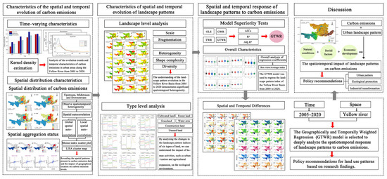
Figure 1.
Technology roadmap.
2. Study Area and Data Sources
2.1. Overview of the Study Area
The Yellow River, originating from the Qinghai–Tibetan Plateau, flows west to east across nine provinces in China. Its topography varies considerably across four major geomorphological units—namely the Yellow–Huaihai Plain, the Loess Plateau, the Tibetan Plateau, and the Inner Mongolian Plateau—and plays an important ecological role. As of 2023, it has 29.7% of the country’s total population and 25.1% of the country’s GDP. Therefore, China’s Yellow River Basin has significant ecological and socioeconomic value and has an irreplaceable role in the national development strategy. This research concentrates on the Yellow River Basin and uses prefecture-level cities as the spatial analytic unit. To strengthen the universality of the results, the study samples cover the prefecture-level cities through which the Yellow River mainstream and the first-level tributaries flow, totaling 61 cities. Due to the wide range of basins and the significant differences in natural and socio-economic factors between regions, this study splits the research region into upstream, midstream, and downstream (Figure 2).
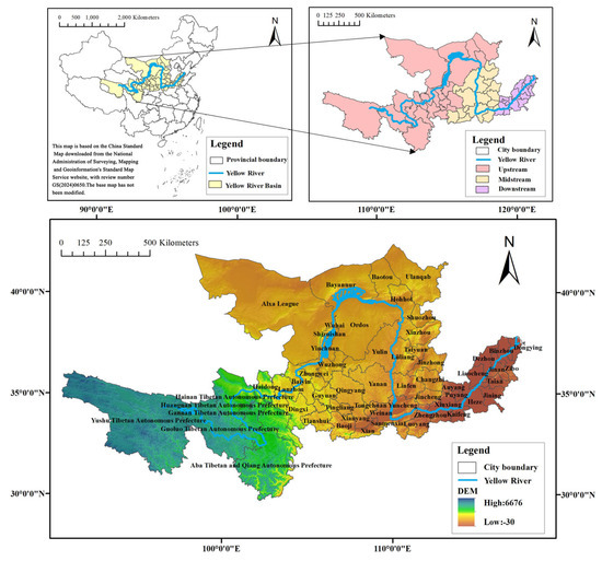
Figure 2.
Location map of the Yellow River Basin.
The upstream area includes 26 prefectural-level cities in Inner Mongolia, Qinghai, Ningxia, Gansu, and Sichuan, which are mostly alpine and arid ecologically fragile areas with more mountains and canyons, inconvenient transportation, and restricted development. The middle reaches of the region include 16 prefecture-level cities in Shaanxi and Shanxi, most of which are loess landscapes with relatively serious soil erosion, rich in energy resources, and relying on heavy industries such as coal and chemicals to develop their economies. The downstream area includes 19 prefectural-level cities in Henan and Shandong, has plains as its main terrain, has a dense population and convenient transportation, and is the highest economically developed region in the basin.
2.2. Data Sources
This study examines the impact of urban landscape patterns on carbon emissions in 61 cities within China’s Yellow River Basin from 2005 to 2020 (Table 1).

Table 1.
Research Data and Sources.
3. Research Methodology
3.1. Kernel Density Estimation
Kernel density estimation is a nonparametric approach used to infer the probability density function of an unknown distribution [43], and this approach can visually present the evolution trend of the target variable and reveal its stage distribution characteristics through a frequency distribution graph. This research employs this approach to assess the development of urban carbon emissions and its time-series features in each region of the Yellow River from 2005 to 2020 [44]. Stata 17 was utilized to construct the kernel density map of urban carbon emissions and explore its dynamic evolution trend according to the curve position, wave peak position, and ductility in the map.
In this context, n indicates the number of cities in China’s Yellow River Basin; xi denotes the observed value for each sample, i.e., the carbon emissions of each city; x is the mean of the observed values; h is the bandwidth; f(x) is the kernel density calculation function; and K(x) is the kernel function.
3.2. Spatial Autocorrelation Analysis
Spatial autocorrelation can be classified into two types: global and local, which serve as a metric for assessing the strength of correlation of a phenomenon between neighboring regions. This study analyzes the spatial clustering characteristics of carbon emissions across different periods from 2005 to 2020 at both global and local scales. It examines whether urban carbon emissions in the Yellow River Basin exhibit spatial dependency and identifies the spatial distribution of high-value and low-value clusters.
Global spatial autocorrelation explains the spatial properties of all converging attribute values [45]. Global Moran’s I is founded on the premise of spatial unit homogeneity and is used to reveal the spatial correlation patterns across the entire region. Local spatial autocorrelation is used to identify patterns of spatial clustering or dispersion of variables within a specific region. Local Moran’s I is used to identify spatial clustering or dispersion patterns between a specific city and its neighboring cities [46].
The formula to calculate this index is as below:
Here, n is the number of cities, xi and xj represent the carbon emissions of the i-th and j-th cities, respectively, is the average carbon emissions, and denotes the spatial weight between these two elements.
Moran’s I ranges from −1 to 1: A global value > 0 indicates that carbon emissions are spatially aggregated; A local value > 0 indicates a positive correlation between a city’s emissions and those of its neighboring cities, reflecting spatial clustering. In contrast, Moran’s I < 0 indicates spatial dispersion, while Moran’s I = 0 signifies the absence of spatial dependence.
3.3. Urban Landscape Pattern Index
Landscape pattern indices serve as essential tools for assessing the properties of landscape formations, providing insights into their composition and spatial evolution. This study employs a common six-category land use classification system, encompassing cropland, forest land, grassland, water bodies, construction land, and unutilized land. Using Fragstats 4.2 software, landscape pattern indices were calculated based on this classification system. In selecting indicators, we drew upon relevant research findings [47,48]. The landscape pattern indices employed in these studies are widely applied in ecological effect and carbon emission analyses, possessing a mature theoretical and practical foundation. Simultaneously, considering the diverse land use types and landscape structural characteristics of the Yellow River Basin, along with data availability and spatial resolution constraints, this study selected 12 indices across six categories: scale, fragmentation, clustering, heterogeneity, shape complexity, and diversity (Table 2). These were used to analyze landscape pattern changes in the Yellow River Basin at both the landscape level and typological level. This approach aims to reveal the overall landscape structure and spatial pattern characteristics of different land types, with the selected indices serving as explanatory variables in subsequent GTWR analyses. It should be noted that the analysis in this study focuses solely on the impact of landscape patterns on carbon emissions, excluding other factors that may influence emissions. This approach aims to highlight the direct effect of landscape patterns themselves on carbon emissions.
Table 2.
Description of landscape pattern indicators.
3.4. Geographically and Temporally Weighted Regression (GTWR) Model
Traditional Geographically Weighted Regression (GWR) models can reveal spatial heterogeneity among variables, but they are limited to cross-sectional data and struggle to capture dynamic changes over time. To address this, this study employs the GTWR model, which extends GWR by incorporating a temporal dimension to better characterize the spatiotemporal relationship between urban carbon emissions and landscape pattern indices [49]. The GTWR is better at expressing the spatial–temporal link between dependent and independent variables [50], and its calculation formula is as below:
Here, (,) represents the latitude and longitude coordinates of the i-th city, denotes the observation time, yi denotes the value of the dependent variable of the i-th city, and xik represents the k-th explanatory variable of the i-th city, where the explanatory variables are the landscape pattern indices selected in Table 2. ,,) represents the regression constant for the i-th city, and (,,) represents the regression coefficient of the k-th explanatory variable for the i-th sample point; is the model error term. By incorporating urban coordinates and time-series information, GTWR can reveal the spatiotemporal effects of landscape patterns on carbon emissions.
4. Results
4.1. Characteristics of the Spatial and Temporal Evolution of Carbon Emissions
4.1.1. Time-Varying Characteristics
This study calculates overall and regional carbon emissions from 2005 to 2020 in order to observe their time-varying characteristics. Through observation, the total carbon emissions show a continuous increase from 1411.76 Mt in 2005 to 2851.81 Mt in 2020, with a significant overall increase.
According to the Formulas (1) and (2), the carbon emission density curves were calculated to reveal the temporal evolution characteristics. The carbon emission level in the upstream area was concentrated in the lower value range in 2005, with a higher peak of the density curve and denser data. The carbon emission density curve’s peak progressively declines over time, and the trailing tail on the right side is prolonged, indicating that the carbon emission level tends to be dispersed in the region, and the proportion of cities in the high-value zone increases. The midstream region has the highest total carbon emissions, with emission levels showing a gradual increase after 2010. The top of the density curve gradually shifts to the right, and the high carbon emission zone significantly expands, and the density distribution further broadens by 2015 and 2020, indicating that the contribution of the high-emission region increases, and the carbon emission is highly differentiated between regions [51]. Within the research time, the wave peak in the downstream area migrated dramatically to the right, indicating that the region’s urban carbon emissions had undergone a considerable overall increase Figure 3. It should be noted that the bandwidths of the kernel density estimate for the upstream, midstream, and downstream regions are 6.2799, 8.1669, and 10.9811, respectively. This indicates that upstream cities exhibit the greatest variation in carbon emissions, midstream regions are in a transitional state, while downstream regions show relatively greater equilibrium. From a comprehensive point of view, carbon emission levels in all areas are on an upward trend overall, although the degree of rise varies, and the overall spatial gradient distribution of “upstream is low, midstream is high, and downstream is medium” occurs.
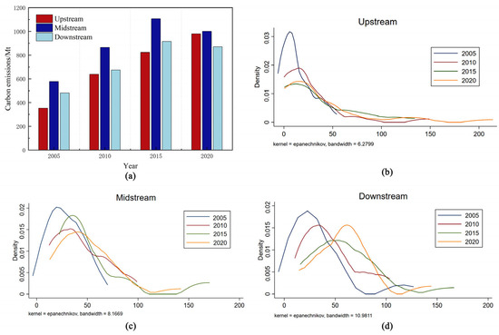
Figure 3.
Characterization of temporal changes in carbon emissions. (a) Statistical map of carbon emissions in the Yellow River basin region; (b) Upper Yellow River Basin kernel density curve; (c) Histogram of the central Yellow River Basin kernel density curve; (d) Lower Yellow River Basin kernel density curve.
4.1.2. Spatial Distribution Characteristics
From the viewpoint of spatial distribution, the carbon emissions exhibit a clear two-level distribution, with the high-value areas mostly found in key economic zones in the middle and lower reaches, especially in the areas with intensive energy industries, such as Ordos, Jinan, and other cities; the low-value area is mainly centered in the upper reaches, such as Qinghai and Gansu. Due to the limitations of natural conditions and the rigid requirements of ecological environmental protection, carbon emissions show a gradient of distribution from low to high from the upstream to the downstream, and from 2005 to 2020, the area of the high-value zone is expanding, especially in the middle and downstream regions, spreading from the core cities to the neighboring cities; the area of the low-emission zone is gradually shrinking to the medium emission level. At the same time, the scope of low-emission zones gradually shrinks and transitions to the medium emission level (Figure 4).
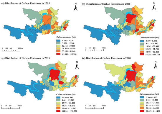
Figure 4.
Characterization of the spatial distribution of carbon emissions. (a) Carbon emissions distribution in 2005; (b) carbon emissions distribution in 2010; (c) carbon emissions distribution in 2015; (d) carbon emissions distribution in 2020.
Urban carbon emissions are very spatially dependent [52]. To identify the most suitable econometric model, this study employed Moran’s I to analyze the spatial autocorrelation [53]. Based on Formulas (3) and (4), Moran’s indices were calculated, and Geoda 1.22 software was used to measure the global and local Moran’s index (Figure 5). The findings indicate a positive spatial correlation in urban carbon emissions during the period from 2005 to 2020. The process of increasing from 0.205 in 2005 to 0.340 in 2020 reflects the increased spatial agglomeration. Analysis of the local LISA clustering diagrams reveals that the “high–high concentration” zone primarily exists in the Inner Mongolia and Shandong provinces in the midstream and downstream, and the range is gradually expanding; the “low–low concentration” zone is stably dispersed across the upstream Gansu and Qinghai provinces. The “low–high concentration” and “high–low concentration” zones are primarily situated at the intersection of the middle and lower reaches, and their distribution is relatively scattered. On the whole, carbon emissions in the upstream area are dominated by “low–low concentration,” and the overall low–carbon development trend is steady; the midstream area is the core area of “high–high concentration”; and the spatial concentration in the downstream area is not obvious, but the overall trend is toward high-concentration development.
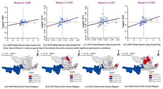
Figure 5.
Scatterplot of global Moran index and local LISA clustering. (a.1–d.1) Global Moran’s I scatter plots for 2005, 2010, 2015, and 2020. (a.2–d.2) Local LISA clustering maps for 2005, 2010, 2015, and 2020.
4.2. Characteristics of Spatial and Temporal Evolution of Landscape Patterns
4.2.1. Characteristics of Changes in the Landscape Level
The landscape level focuses on the overall landscape of the whole landscape of the studied region and reflects the global aspects of the landscape spatial pattern. This study calculated landscape pattern indices at the landscape level for the Yellow River basin and analyzed the rate of change in these indices over five-year periods (Table 3). Based on this analysis, we then plotted the distinctive features of these changes at the landscape level (Figure 6). Overall, the changes in the indices in this period show obvious spatial and temporal heterogeneity.
Table 3.
Average Rate of Change for Landscape Pattern Indices Across Stages.
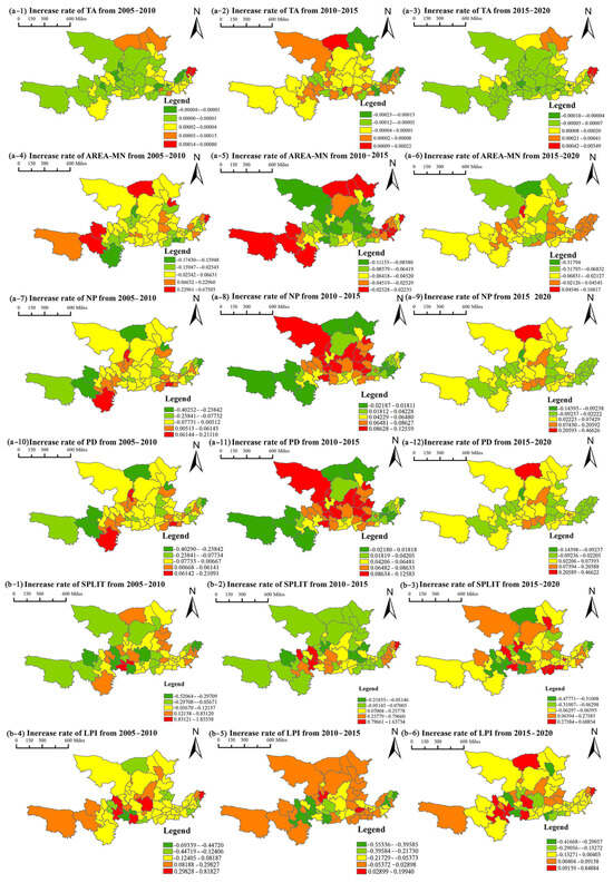
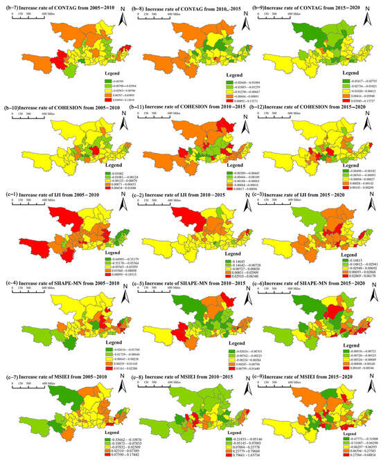
Figure 6.
Characteristic analysis of landscape-level pattern index changes.
In terms of scale, the TA index indicates a general decreasing tendency, with an average yearly rate of change for all cities being less than 1 percent, which is a relatively small change. The average rate of change for AREA-MN declined from 4.74% to −3.34%, with a gradual reduction in the scale of the landscape unit.
Regarding fragmentation, NP and PD have changed from large-scale negative growth to large-scale positive growth, with the average rate of change rising from −3.01% to 3.91% and 3.89%, respectively, while the average rate of change in SPLIT has fallen from 6.69% to 4.51%. Among these indices, NP and PD exhibited more pronounced growth in the midstream region, whereas their changes in the upstream and downstream regions were relatively moderate. Meanwhile, SPLIT showed a decreasing trend in the upstream region, a growing trend in the midstream, with little fluctuation in the downstream zone.
For landscape aggregation, LPI, CONTAG, and COHESION exhibited varying degrees of change. The average rate of change for LPI declined from 2.25% to 1.08%, with a growing trend in the upstream region, a declining trend in the midstream, and minimal variation downstream. Meanwhile, the average rate of change for the CONTAG index rose from −0.95% to −0.80%, indicating a slight reduction in its negative growth. In contrast, the COHESION index saw its average rate of change decrease from −0.02% to −0.04%. Although the overall changes in CONTAG and COHESION were relatively minor, the upstream region displayed a noticeable upward trend. This was particularly evident from 2010 to 2015, during which COHESION experienced significant positive growth in the upstream area.
With respect to heterogeneity and shape complexity, the average rate of change in IJI rose from −1.52% to 0.32%, and growth is focused in the upstream region, whereas the mid- and downstream zones show minimal change. The average rate of change in SHAPE-MN fell from 0.01% to −0.16%, with a relatively small overall change, but with a significant positive increase in the upstream region between 2010 and 2015.
In terms of diversity, MSIEI demonstrates an increased trend in diversity, with the average rate of change increasing from 0.28% to 2.06%. Between 2010 and 2020, the lower and intermediate reaches experienced the greatest increase, while the upper reaches exhibited less change.
In conclusion, the overall decline in landscape scale occurs across regions. The upstream area has decreased fragmentation, increased aggregation and heterogeneity, and the landscape patch pattern tends to be naturalized; the midstream area has increased landscape fragmentation, decreased aggregation, and increased landscape diversity, but the pattern tends to be simpler; and the downstream area has an overall stable landscape pattern, increased landscape diversity, and a more balanced spatial distribution of landscape types.
4.2.2. Characteristics of Type-Level Changes
Within a certain range, the transformation between the same patch type and the transformation of different patch types are its more prominent expression features [54]. This dynamic landscape structural feature affects the stability and functional expression of the landscape pattern [55]. The type-level hierarchy focuses on the spatial distribution characteristics of specific landscape types (e.g., construction land, arable land, forest land, grassland, etc.) to reveal the spatial distribution patterns of different types of land and their impacts on the changes in the overall landscape pattern. In order to further explore the landscape dynamic characteristics of different regions, this study calculated the landscape pattern index at each regional type level and accordingly plotted the change characterization map (Figure 7). Furthermore, to avoid the impact of numerical scale disparities on the analysis findings, CA, AREA-MN, and SPLIT were log-transformed in this study to improve data visualization.
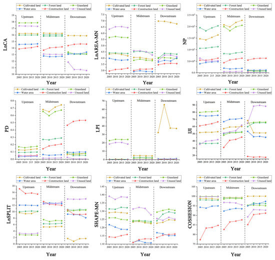
Figure 7.
Characteristics of changes in landscape pattern indices at type level.
In terms of scale change, the CA values of cropland, forest land, and grassland remained relatively stable overall. In contrast, construction land experienced a notable increase in CA values, while unutilized land showed a sharp decline in the downstream region. Additionally, the AREA-MN exhibited a significant decrease in the midstream region.
In terms of fragmentation, grassland and cropland NP and PD values were higher, indicating a stronger degree of fragmentation. The NP and PD values of construction land steadily grow, suggesting a rise in the degree of fragmentation, but its SPLIT value shows an overall decreasing trend, reflecting the evolution of its spatial pattern from dispersed to concentrated. The upstream construction land has the highest SPLIT and the most serious fragmentation, while the downstream has the lowest, and the construction land tends to be contiguous. The SPLIT value of unused land is the highest in the downstream and the lowest in the upstream, indicating that unused land tends to be fragmented in the downstream and more contiguous in the upstream.
In terms of agglomeration, the LPI values for grassland and unutilized land are notably higher in the upstream region, while cropland exhibits relatively high LPI values in the midstream and downstream. Additionally, the LPI of cropland in the downstream area experienced a sharp increase around 2010, followed by a subsequent decline, indicating that the downstream area had experienced a large-scale expansion of contiguous cropland in the period. The COHESION values for construction land and water area rose dramatically, indicating a more compact distribution of construction land and increased spatial agglomeration during the urbanization process.
In terms of heterogeneity and shape complexity, the IJI value of unutilized land rises significantly, reflecting its gradual transformation to other land categories. The IJI value of land for construction in the river’s middle reaches rises similarly, indicating an increase in the spatial interlocking of the two types of land: the IJI values of cultivated land and waters in the river’s lower reaches fall, reflecting a more contiguous spatial pattern. Construction land showed a significant increase in SHAPE-MN values, accompanied by large morphological changes.
In summary, the scope of construction land in the upstream region rose, but there was a high degree of fragmentation, which tended to stabilize with time, and the grassland and unused land’s agglomeration increased, along with increased heterogeneity of unused land. In the midstream, landscape fragmentation was significant; built-up land became more concentrated, interlocking increased, and morphological complexity improved. In the downstream, the scope of unused land resources and cultivated land stabilizes after a short period of expansion, built-up land has the least fragmentation, the contiguity of cultivated land and waters increases, and the overall landscape pattern tends to stabilize.
4.3. Spatial and Temporal Response of Landscape Patterns to Carbon Emissions
4.3.1. Model Superiority Tests
Four models, OLS, GWR, TWR, and GTWR, were employed for analysis and to compare their fitting performance. Before modeling, the variables were tested for covariance using Stata 17, and the results showed that all variables had VIF < 10 and there was no multicollinearity problem. The model fitting results indicated that the OLS exhibited the highest AICc value and the lowest R2, reflecting a limited capacity to explain the spatial response of landscape patterns and carbon emissions. The GWR model was slightly better on AICc, but both R2 and Adj. R2 showed that the GTWR fitting effect was much superior to the other models (Table 4). The GTWR considers both spatial and temporal heterogeneity and captures spatial effects over time, which better reflects its applicability in macro-scale spatial pattern studies. This comparison also demonstrates that the results of the GTWR model exhibit robustness and reliability across different models.
Table 4.
Comparison of regression model goodness of fit and results.
4.3.2. Overall Characteristics of Landscape Pattern Response to Carbon Emissions
According to Formula (5), the GTWR was utilized to regress the data from 2005 to 2020, and box plots were used to show the characteristics of its changes (Figure 8).
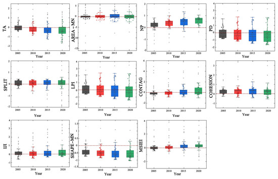
Figure 8.
Box Plot of GTWR Coefficients 2005–2020.
Overall, the landscape pattern indices NP, IJI, SPLIT, COHESION, and MSIEI exhibited positive correlations with carbon emissions, and the strength of these correlations increased over time. In contrast, TA, PD, LPI, and SHAPE-MN generally showed negative correlations. The regression coefficients of AREA-MN exhibited bidirectional effects, while the CONTAG index shifted from entirely negative correlations in 2005 to entirely positive correlations in later years.
In order to present a finer picture of the high and low regression coefficients, and taking into account that the spatial distance between the regions is far and their landscape pattern and carbon emission relationship may be quite different, this study used the method of partition statistics for comparison (Table 5). Before the comparative analysis, the regression indices were first averaged separately for each region to ensure the holistic assessment of interregional differences. Specifically, according to the tertile division criterion [56], the indices with average regression coefficients in the first 33.3% were classified as the high-value group, which meant that they had a considerable influence on carbon emissions; indices between 33.3% and 66.7% were classified as the medium-value group, which meant that they had an appropriate influence on carbon emissions, but relatively weaker; and indices in the latter 33.3% were classified as the low-value group, which implied that they had a small impact. Compared to traditional grouping methods based on mean and standard deviation, the quantile method avoids the interference of extreme values and provides a more balanced reflection of the relative levels and differences among various indicators.
Table 5.
Mean regression indices of GTWR in the upper, middle and lower reaches.
Based on this categorization criterion, in the upstream region, in the upstream region, NP, CONTAG, IJI, and SHAPE-MN indices significantly influence carbon emissions, followed by TA, PD, COHESION, and MSIEI, while AREA-MN, SPLIT, and LPI exert the least influence. In the midstream region, AREA-MN, NP, IJI, and SHAPE-MN have the highest impact, followed by PD, SPLIT, COHESION, and MSIEI, while TA, LPI, and CONTAG have the lowest impact. In the downstream area, AREA-MN, NP, PD, and SHAPE-MN had the highest impact, followed by TA, LPI, COHESION, MSIEI, SPLIT, CONTAG, and IJI, which had the lowest impact. This analysis indicates that the landscape pattern index has different patterns of influence on carbon emissions in different regions, suggesting that urbanization, land-use composition, and ecological characteristics vary significantly across different regions in both spatial and temporal dimensions. Meanwhile, Table 5 indicates the statistical significance of each regression coefficient, enabling a more intuitive assessment of the reliability of each landscape pattern index’s impact on carbon emissions. Except for the midstream MSIEI, most regression coefficients are significant, suggesting that these landscape pattern indices exert statistically reliable effects on carbon emissions. This also indicates that landscape boundary complexity exerts a weaker influence on carbon emissions in midstream regions, reflecting regional differences.
4.3.3. Spatial and Temporal Differences in the Response of Landscape Patterns to Carbon Emissions
To obtain deeper insights into spatiotemporal variations in how landscape patterns affect carbon emissions, this research used ArcGIS 10.8 to display and map the regression coefficients produced from the GTWR model (Figure 9).
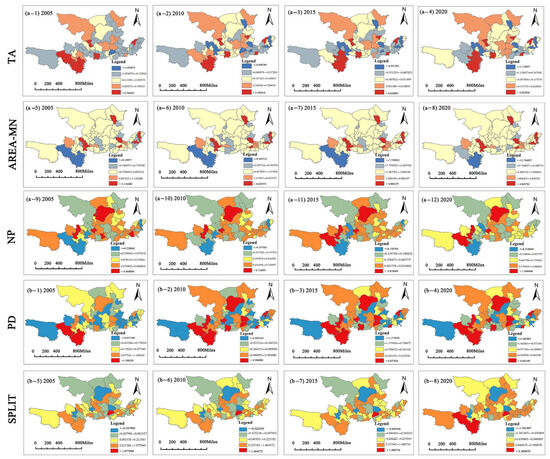
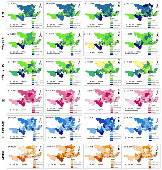
Figure 9.
GTWR model regression coefficient analysis.
Among the indices in the scale category, TA was mainly negatively correlated in the downstream at the beginning of the study, while the direction and intensity of correlation varied greatly in the upstream and midstream regions, exhibiting spatial variations across different regions. With the passage of time, the negative correlation of TA expanded over time, eventually encompassing the entire watershed. AREA-MN was mainly negatively correlated in the midstream region, while the upstream and downstream did not have obvious regional characteristics, and the strength of the correlation was enhanced with the change in time.
In the fragmentation index, NP had the largest range of positive correlations in the middle reaches, expanding over time to the upstream and downstream regions, while the negative correlation effect in the upstream Sichuan and Gansu is gradually weakened. PD is negatively correlated in the downstream, and the negative correlation effect is further strengthened with time, while the correlation direction and strength differ greatly between the upstream and middle reaches. SPLIT exhibits a positive correlation, except in the upstream areas of Qinghai, Ningxia, and Inner Mongolia, as well as some cities in Shanxi along the middle reaches, where a negative correlation is observed.
In the agglomeration index, LPI shows a positive correlation in the midstream region as a whole, with no obvious trend in the lower reaches, while upstream Inner Mongolia, Ningxia, and Sichuan mainly exhibited a positive correlation, while there are significant disparities in the direction and strength of correlation among cities in Qinghai and Gansu. With the passage of time, the spatial change is small, but the intensity of negative correlation is enhanced. CONTAG is mainly negatively correlated in the early stage, and only positive correlation exists in upstream Qinghai and Sichuan. After 2010, the negative correlation effect in the upstream is enhanced, whereas the positive correlation in the middle and downstream extends and strengthens. COHESION is mainly positively correlated in the early stage, and local negative correlation is demonstrated in Inner Mongolia and Gansu, whereas the intensity of positive correlation in the downstream is the largest. With the passage of time, the spatial difference changes less, but the intensity is enhanced.
In the heterogeneity and shape complexity indices, the spatial heterogeneity of IJI is stronger in the early stage, with most regions in the basin showing positive correlation and only Qinghai, Gansu, and Shandong showing a small amount of negative correlation. With the passage of time, the strength of positive correlation in the basin is significantly enhanced, the strength of negative correlation is weakened, and the spatial variation is relatively small. SHAPE-MN is negatively correlated in the early stage as a whole, and only some cities in Shanxi are positively correlated. As time progresses, the strength of the negative correlation increases, while the spatial distribution pattern remains largely stable.
In the diversity index, MSIEI’s early positive and negative correlations are more balanced, with both positive and negative correlations present. However, over time, many cities in the upstream and midstream shift from a significant negative correlation to a significant positive correlation. This shift enhanced the positive influence of MSIEI, with the strength of the positive correlation notably increasing. The changes in the downstream area are relatively small, and the influence pattern is more stable.
5. Discussion
5.1. Spatial and Temporal Changes in Landscape Patterns and Carbon Emissions in the Yellow River Basin
5.1.1. Spatial and Temporal Changes in Carbon Emissions
Carbon emissions as a whole exhibit a spatial pattern of low in the upstream, high in the middle reaches, and medium in the downstream, and the upstream area exhibits a ‘low–low’ cluster, whereas the middle reaches exhibit a ‘high–high’ cluster. Carbon emissions across the entire watershed exhibit a trend of peaking in the middle and lower reaches. This pattern not only reflects differences in natural geographical conditions but also results from the combined effects of socioeconomic development models and policy orientations.
The upstream region of the Yellow River, characterized by complex terrain and poor transportation infrastructure, exhibits lower levels of industrialization. Combined with national policies such as the Grain-for-Green Program, the Grassland Restoration Program, and the ecological red line system, these factors have effectively restricted the expansion of construction land while enhancing the carbon sink functions of grasslands and forests. Consequently, the upstream regions have long maintained low emissions. The mid-stream region of the Yellow River serves as China’s quintessential energy and heavy industrial base. The concentration of high-energy-consuming industries—including coal, power generation, metallurgy, and coking—remains the primary driver of persistently elevated carbon emissions. Despite recent advances in green transformation, high-carbon industries continue to dominate, sustaining high emission levels. For instance, the clustered distribution of coal-fired power plants and coking industries in regions like Shanxi and Shaanxi directly fuels energy consumption and land fragmentation, creating a “high–high clustering” pattern. Downstream regions of the Yellow River, such as Jinan and Zhengzhou, exhibit higher urbanization levels but are dominated by high-end services and high-tech manufacturing. Consequently, their carbon emissions intensity per unit of GDP is significantly lower. Through gradual industrial restructuring, these areas have effectively controlled carbon emission growth rates. These findings align with scholar Tian Mingjie’s research on land-use carbon emissions in the Yellow River basin [57], further revealing the regionally differentiated drivers within China’s Yellow River basin: upstream regions are dominated by ecological policies, midstream areas are driven by energy industries, while downstream zones exhibit dual effects of industrial upgrading and land management.
5.1.2. Spatial and Temporal Changes in Landscape Patterns
Studies have shown that in the upstream area of the Yellow River, fragmentation decreases, while aggregation and heterogeneity increase; the landscape tends toward naturalization. The extent of built-up land has expanded, accompanied by increased fragmentation, and grassland and unused land show stronger agglomeration. In the midstream region, the landscape fragmentation increases, the aggregation decreases, the diversity increases but the form tends to be simpler, the level of fragmentation of the construction land decreases, the spatial distribution evolves from dispersed to concentrated, and the complexity of the form increases. In the downstream area, the landscape pattern is generally stable, diversity is increased, the distribution of types is more balanced, unused land is reduced, cultivated land and water contiguity are enhanced, and the fragmentation level of construction land is at its lowest, exhibiting an overall stable trend.
The upstream area of the Yellow River, located in the western parts of the Qinghai–Tibet Plateau and the Loess Plateau, is characterized by complex terrain and fragile ecosystems, yet rich in vegetation diversity and strong water conservation capacity. In recent years, national ecological protection policies have significantly improved grassland and wetland systems, enhancing the connectivity of natural landscapes, reducing fragmentation, and increasing ecological coherence. However, due to varying restoration rates across different regions, landscape heterogeneity has increased, resulting in an overall trend toward naturalization. Additionally, constrained by terrain and development conditions, although construction land has expanded, fragmentation remains pronounced; simultaneously, grassland restoration and the reorganization of unused land have strengthened landscape aggregation.
The midstream region of the Yellow River exhibits intensified landscape fragmentation due to energy development and urban expansion. Against the backdrop of the “Western Development Strategy,” coal mining, energy base construction, and industrial park development have driven large-scale land-use changes, disrupting the integrity of ecological patches and reducing their aggregation. Simultaneously, accelerated urbanization and industrial clustering have shifted construction land from dispersed to concentrated patterns. While superficially mitigating local fragmentation, this trend—marked by increasingly regular landforms and intensified land-use mixing—has resulted in a landscape characterized by “increased diversity but reduced complexity.” This phenomenon reflects the inherent contradiction in landscape patterns under high-intensity development: economic growth accompanied by mounting ecological pressures.
Downstream regions of the Yellow River, as the most economically developed areas within the basin, have reached a mature stage of urbanization with stricter land use controls. Under policies such as the “Central Plains Urban Cluster Development Plan” and the “Yellow River Delta Ecological Protection Project,” construction land expansion has primarily occurred through intensification and contiguous development. This has strengthened the contiguity of farmland and water bodies while significantly reducing unutilized land. While the overall landscape pattern remains stable, diversity gains in ecological corridors and wetland restoration areas stem primarily from ecosystem recovery. Conversely, in rapidly urbanizing zones, diversity increases as a result of functional mixing within construction land.
These findings largely align with Wang Qianxu’s research on landscape pattern evolution in the Yellow River Basin based on optimal scale [58]. However, this study further reveals the central role of policy direction and industrial development in landscape pattern evolution. Notably, it uncovers the contradictory trend of “regularization versus mixed use” in the middle reaches and the dual effects of diversity changes in the lower reaches, expanding the perspective of existing research.
5.2. Spatial and Temporal Response Mechanisms of Landscape Patterns to Carbon Emissions
5.2.1. Basin-Wide Landscape Pattern Response Mechanisms
In general, various attributes of the landscape pattern exert different driving mechanisms on carbon emissions. Specifically, the NP, IJI, SPLIT, COHESION, and MSIEI show a positive correlation; TA, PD, LPI, and SHAPE-MN are negative as a whole, and the regression coefficients of AREA-MN show a significant two-sidedness, while the CONTAG index, the negative correlation, gradually becomes positive. This conclusion aligns with findings from the study on the urban form and carbon emissions in the Changsha-Zhuzhou-Xiangtan region [59]. However, unlike the Changsha-Zhuzhou-Xiangtan area, where compact urban expansion predominates, the Yellow River Basin is more typically driven by factors such as farmland fragmentation and energy development activities. This makes the landscape pattern more sensitive to carbon emissions. From the perspective of regional differences, NP, CONTAG, IJI, and SHAPE-MN had the greatest influence in the upstream area of the Yellow River; AREA-MN, NP, IJI, and SHAPE-MN indices had the greatest influence in the midstream area of the Yellow River; and AREA-MN, NP, PD, and SHAPE-MN had the greatest influence in the downstream area of the Yellow River. The findings suggest that landscape fragmentation and shape complexity have significant impacts on the watershed as a whole. Additionally, there is clear spatial heterogeneity in how different landscape pattern indices influence carbon emissions. These differences stem not only from variations in natural environments but are also closely tied to regional economic functions and industrial policies. For instance, energy development strategies in midstream regions of the Yellow River and rapid urbanization in downstream areas are intensifying the interaction between landscape patterns and carbon emissions. The effects of these patterns vary across regions, and they evolve over time. The findings are consistent with relevant studies in the Yangtze River Economic Belt [60]. However, this study places greater emphasis on the dynamic evolution driven by the combined forces of energy policy and urban expansion.
5.2.2. Upstream Response Mechanisms
The upstream region of the Yellow River maintains a well-preserved ecosystem, mainly consisting of natural landscapes such as forests and grasslands [61]. Changes in its landscape pattern mainly affect carbon emissions through the ecological barrier effect. The TA index is negatively correlated, indicating that large-scale landscape patterns contribute to the enhancement of carbon sequestration and sink functions. The direction in which the NP, PD, and SPLIT impact carbon emissions varies by area. For example, in Qinghai and other places, due to strict restrictions on land use, the growth of construction land is well managed, and the influence of landscape fragmentation remains limited. However, in some areas with active resource development, such as mineral and hydropower development or urban expansion areas, the degree of landscape fragmentation has increased significantly, driving carbon emissions growth. This indicates that differences in Yellow River upstream emissions are determined not only by natural ecological barriers but also influenced by resource-based industrial policies and infrastructure development priorities. The overall negative correlation between LPI and CONTAG has strengthened, while the overall positive correlation between COHESION has also increased. This indicates that as landscape patch size and aggregation increase, ecological connectivity improves, contributing to the formation of stable ecosystems and effectively suppressing carbon emissions. Additionally, the enhanced positive correlation between IJI and the enhanced negative correlation between SHAPE-MN suggest that increased mixing and interweaving of landscape types promote carbon emissions, while the tendency toward regularized patch shapes reflects landscape structure optimization resulting from land reclamation or energy development, which plays a part in lowering carbon emissions. MSIEI changed from being negatively to positively associated, demonstrating a decrease in carbon emissions during the initial phases of vegetation regeneration. However, with the increase in infrastructure construction and agricultural land use, landscape diversity actually promoted carbon emissions in the later stages, reflecting a phased transition from an “ecology-dominated” to a “construction-dominated” phase in the Yellow River upstream region.
5.2.3. Midstream Response Mechanisms
The midstream region of the Yellow River is a major energy and industrial foundation, and the impact is mostly reflected in the driving effects of energy industry development and land use changes. The negative correlation between TA and the AREA-MN index indicates that enhanced landscape connectivity helps improve carbon sink function and reduce carbon emissions; however, the reduction in large-scale patches (such as forest and farmland fragmentation) often leads to increased carbon emissions, which is similar to Zhao’s findings that contiguous landscapes help improve ecological hydrological functions [62]. NP and SPLIT indices show a positive correlation, indicating that the large-scale distribution of coal mining, coking industries, and related energy sectors has led to highly fragmented landscapes, thereby driving increased carbon emissions. Although economic transformation and land consolidation have alleviated the fragmentation trend in some areas, the overall fragmentation trend remains difficult to reverse. The PD index shows no significant spatial differences, but LPI, CONTAG, and COHESION are positively correlated, indicating that as urbanization accelerates and energy consumption increases, land use concentration rises, leading to a concentrated increase in carbon emissions. IJI is positively correlated, while SHAPE-MN is negatively correlated, indicating that urban expansion leads to more regular land use patterns, but the mixed development of industry, agriculture, and urban areas exacerbates carbon emissions. This conclusion aligns with relevant studies in China’s Pearl River Delta region [63]. However, unlike the Pearl River Delta region, which is dominated by manufacturing and export-oriented economies, carbon emissions in the central regions of the Yellow River midstream area are more heavily influenced by resource-based industries and constrained by coal consumption patterns. MSIEI shifts from a negative to a positive correlation, reflecting a transition from an ecology-dominated landscape to one dominated by urban and industrial landscapes, which increases carbon emissions.
5.2.4. Downstream Response Mechanisms
The downstream region of the Yellow River is heavily urbanized and serves as a key agricultural production zone. The impact is primarily manifested through the interplay between urban spatial configuration and industrial structure. The TA index is negatively correlated, indicating that contiguous agricultural and ecological land use reduces the diffusion effect of carbon emissions, which accords with Du’s conclusion that dispersed farmland exacerbates carbon emissions [64]. The positive correlation of NP and SPLIT and the strengthening of the negative correlation of PD indicate that with the increase in urban density, the towns and the ecological land use in the vicinity, agricultural land boundaries become more fragmented, and land use imbalance and carbon emission diffusion intensify. This effect is particularly pronounced in the Yellow River urban agglomeration, where rapid urban sprawl not only encroaches on farmland but also intensifies transportation and energy consumption, thereby amplifying carbon emissions. At the same time, although PD has declined in some areas due to land consolidation and infrastructure improvement. CONTAG and COHESION are positively correlated, while LPI shows a relatively balanced positive and negative correlation, reflecting the industrial agglomeration effect of optimizing the energy structure. However, the expansion of construction land in some regions still brings carbon emission pressure [48], causing the LPI to show differentiated trends in different regions. MSIEI shows significant spatial differentiation across different regions. In ecological conservation areas, such as the Yellow River Ecological Corridor, the increase in landscape diversity stems from the restoration of natural ecosystems, which helps enhance carbon sink functions and reduce carbon emissions. In rapidly urbanizing areas, however, the increase in landscape diversity is largely attributable to the growth of construction land and increased mixed use, which has actually exacerbated carbon emissions, demonstrating a certain dual effect. Compared with existing studies, this research reveals that the MSIEI in the Yellow River downstream region not only reflects two distinct pathways—“ecological restoration” versus “urban expansion”—but also shows that under identical index values, its carbon emission effects diverge significantly depending on socioeconomic contexts. This finding highlights the nonlinear functioning of landscape pattern indicators under different development models.
5.3. Policy Recommendations
In upstream regions of the Yellow River, efforts to restore grasslands through grazing cessation and ecological rehabilitation projects should continue, minimizing human disturbance. Concurrently, delineate the “Three Zones and Three Lines” and urban development boundaries, establishing tiered buffer zones along the outer edges of red lines while strictly prohibiting new large-scale development projects. Integrate scattered villages and towns around central hubs to control spillover construction in sensitive areas like gorges and steep slopes, preserving landscape connectivity and reducing land use fragmentation. Simultaneously, vigorously promote ecological animal husbandry and green organic agriculture to mitigate overgrazing. Strictly limit new mineral resource development and high-energy-consumption projects, particularly coal mining and extensive non-ferrous metal smelting—to ensure stable regional carbon sink functions while enhancing grassland and wetland connectivity.
In the middle reaches of the Yellow River, prioritize optimizing urban spatial patterns to reduce land fragmentation and promote compact, polycentric urban agglomeration development. Renovate old urban areas through “ecological restoration + industrial upgrading” to avoid incremental carbon emissions from disorderly expansion. Simultaneously, strengthen soil and water conservation, particularly in the Loess Plateau region, to mitigate erosion. Industrial policies should implement a “coal reduction, greening enhancement, carbon reduction” strategy to lower the consumption share of high-carbon energy. Specifically, phase out typical high-carbon energy facilities such as small-scale coal-fired power plants, coking plants, cement clinker production lines, and energy-intensive chemical installations. Simultaneously, eliminate outdated capacity in industries like steel and building materials, accelerating the exit of enterprises with low energy efficiency. Promote regional industrial restructuring and upgrading by developing new energy industries and establishing efficient clean energy utilization systems.
In downstream regions of the Yellow River, focus should be placed on building multi-centered urban clusters, optimizing urban spatial layouts, and curbing excessive expansion of core cities. Strengthen ecological conservation of the Yellow River Delta wetlands to safeguard critical ecological barrier functions. Accelerate the development of rail transit and smart transportation systems to increase public transit usage and reduce carbon emissions in the transportation sector. Concurrently, expedite the transition to green, low-carbon industries by promoting the transformation of manufacturing toward smart manufacturing, high-end services, and high-tech industries. This will enhance the regional economy’s low-carbon resilience and sustainable development capacity.
6. Conclusions
This study uses the GTWR method to explore the spatiotemporal response mechanism of urban landscape patterns to carbon emissions and provides specific policy recommendations for planning and management. The research findings are outlined below:
- (1)
- Carbon emissions in the Yellow River basin exhibit an overall spatial pattern of “low upstream, high midstream, and moderate downstream,” with pronounced spatial clustering characteristics. The upstream region is constrained by ecological conservation and topography; the midstream region is primarily driven by energy and heavy industry; and the downstream region is regulated by industrial structure optimization and high-end urban development.
- (2)
- The upstream region shows reduced fragmentation, enhanced clustering, and increased heterogeneity; the midstream region experiences heightened landscape fragmentation, reduced aggregation, and increased diversity; and the downstream region maintains overall landscape stability with enhanced diversity.
- (3)
- Landscape pattern indices exhibit distinct heterogeneity in their impact on carbon emissions: patch number, interlaced adjacency, separation index, connectivity index, and modified Simpson’s evenness correlate positively with emissions, while landscape area, patch density, maximum patch index, and mean shape index correlate negatively. Average patch area influences distribution equilibrium, while the sprawl index exhibits a nonlinear relationship. The impact of different regional landscape patterns on carbon emissions varies: the negative effect of landscape area intensifies in the upstream region, while the diversity shifts from negative to positive. The negative effect of patch density increases in the downstream region, and the diversity index transitions from negative to positive in the upstream region but remains stable in the downstream region.
- (4)
- Develop differentiated carbon reduction strategies based on regional variations: Upstream: Strengthen ecological conservation and spatial constraints. Midstream: Optimize urban form and enhance energy efficiency. Downstream: Promote industrial restructuring and spatial optimization.
Although this study has achieved some results at the regional level, there are still some limitations that need to be improved. First, while the study analyzes the entire Yellow River basin to reveal macro-level patterns, its exploration of regional heterogeneity remains insufficient. A more granular spatial division could be adopted—for instance, expanding from the prefecture-level city scale to the county level, or even employing grid-based analysis—to achieve higher-resolution spatial insights. Second, the temporal scope of this study primarily focuses on the past 15 years. While this period reflects certain temporal patterns, its relatively short duration limits in-depth analysis of longer-term historical trends and dynamics. Therefore, incorporating longer time series data and employing multi-model validation methods could further enhance the scientific rigor and generalizability of the conclusions.
Author Contributions
J.H.: Conceptualization, Data Curation, Writing—Review & Editing. Y.D.: Methodology, Software, Investigation, Writing—Original Draft. Y.M.: Visualization, Supervision. D.L.: Conceptualization, Supervision. J.Y.: Formal Analysis, Validation. Z.M.: Investigation, Supervision. All authors have read and agreed to the published version of the manuscript.
Funding
This research was funded by the Key R&D and Promotion Program of Henan Province (Soft Science), grant number 232400410199, and the Humanities and Social Sciences Research Project of the Henan Provincial Department of Education, grant number 2024ZZJH249.
Institutional Review Board Statement
Not applicable.
Informed Consent Statement
Not applicable.
Data Availability Statement
Data will be made available on request.
Conflicts of Interest
The authors declare that they have no conflicts of interest.
References
- Houghton, R.A.; House, J.I.; Pongratz, J.; Van Der Werf, G.R.; Defries, R.S.; Hansen, M.C.; Le Quéré, C.; Ramankutty, N. Carbon emissions from land use and land-cover change. Biogeosciences 2012, 9, 5125–5142. [Google Scholar] [CrossRef]
- Le Quéré, C.; Raupach, M.R.; Canadell, J.G.; Marland, G.; Bopp, L.; Ciais, P.; Conway, T.J.; Doney, S.C.; Feely, R.A.; Foster, P. Trends in the sources and sinks of carbon dioxide. Nat. Geosci. 2009, 2, 831–836. [Google Scholar] [CrossRef]
- Harper, A.B.; Powell, T.; Cox, P.M.; House, J.; Huntingford, C.; Lenton, T.M.; Sitch, S.; Burke, E.; Chadburn, S.E.; Collins, W.J. Land-use emissions play a critical role in land-based mitigation for Paris climate targets. Nat. Commun. 2018, 9, 2938. [Google Scholar] [CrossRef] [PubMed]
- Gao, H.; Sabo, J.L.; Chen, X.; Liu, Z.; Yang, Z.; Ren, Z.; Liu, M. Landscape heterogeneity and hydrological processes: A review of landscape-based hydrological models. Landsc. Ecol. 2018, 33, 1461–1480. [Google Scholar] [CrossRef]
- Zhang, Y.; Wang, Y.; Ding, N. Spatial effects of landscape patterns of urban patches with different vegetation fractions on urban thermal environment. Remote. Sens. 2022, 14, 5684. [Google Scholar] [CrossRef]
- Liu, Y.; Zhao, J.; Zheng, X.; Ou, X.; Zhang, Y.; Li, J. Evaluation of biodiversity maintenance capacity in forest landscapes: A case study in Beijing, China. Land 2023, 12, 1293. [Google Scholar] [CrossRef]
- Xiong, Y.; Sun, Y.; Yang, Y. Impact of urban green space patterns on carbon emissions: A Gray BP neural network and Geo-Detector analysis. Sustainability 2025, 17, 7245. [Google Scholar] [CrossRef]
- Fischer, J.; Lindenmayer, D.B. Landscape modification and habitat fragmentation: A synthesis. Glob. Ecol. 2007, 16, 265–280. [Google Scholar] [CrossRef]
- Foley, J.A.; DeFries, R.; Asner, G.P.; Barford, C.; Bonan, G.; Carpenter, S.R.; Chapin, F.S.; Coe, M.T.; Daily, G.C.; Gibbs, H.K. Global consequences of land use. Science 2005, 309, 570–574. [Google Scholar] [CrossRef]
- Matveev, A. Evaluating the Land Use Change Carbon Flux and Its Impact on Climate. Master’s Thesis, Concordia University, Montreal, QC, Canada, 2009. [Google Scholar]
- Hansen, J.; Kharecha, P.; Sato, M.; Masson-Delmotte, V.; Ackerman, F.; Beerling, D.J.; Hearty, P.J.; Hoegh-Guldberg, O.; Hsu, S.-L.; Parmesan, C. Assessing “dangerous climate change”: Required reduction of carbon emissions to protect young people, future generations and nature. PLoS ONE 2013, 8, e81648. [Google Scholar] [CrossRef]
- Iftikhar, Y.; He, W.; Wang, Z. Energy and CO2 emissions efficiency of major economies: A non-parametric analysis. J. Clean. Prod. 2016, 139, 779–787. [Google Scholar] [CrossRef]
- Tian, Y.; Zhou, W. How do CO2 emissions and efficiencies vary in Chinese cities? Spatial variation and driving factors in 2007. Sci. Total Environ. 2019, 675, 439–452. [Google Scholar] [CrossRef] [PubMed]
- Li, J.; Huang, X.; Kwan, M.-P.; Yang, H.; Chuai, X. The effect of urbanization on carbon dioxide emissions efficiency in the Yangtze River Delta, China. J. Clean. Prod. 2018, 188, 38–48. [Google Scholar] [CrossRef]
- Li, S.; Zhou, C.; Wang, S.; Hu, J. Dose urban landscape pattern affect CO2 emission efficiency? Empirical evidence from megacities in China. J. Clean. Prod. 2018, 203, 164–178. [Google Scholar] [CrossRef]
- Gudipudi, R.; Fluschnik, T.; Ros, A.G.C.; Walther, C.; Kropp, J.P. City density and CO2 efficiency. Energy Policy 2016, 91, 352–361. [Google Scholar] [CrossRef]
- Christen, A.; Coops, N.; Crawford, B.; Kellett, R.; Liss, K.; Olchovski, I.; Tooke, T.; Van Der Laan, M.; Voogt, J. Validation of modeled carbon-dioxide emissions from an urban neighborhood with direct eddy-covariance measurements. Atmos. Environ. 2011, 45, 6057–6069. [Google Scholar] [CrossRef]
- Baur, A.H.; Förster, M.; Kleinschmit, B. The spatial dimension of urban greenhouse gas emissions: Analyzing the influence of spatial structures and LULC patterns in European cities. Landsc. Ecol. 2015, 30, 1195–1205. [Google Scholar] [CrossRef]
- Massad, R.S.; Lathière, J.; Strada, S.; Perrin, M.; Personne, E.; Stéfanon, M.; Stella, P.; Szopa, S.; Noblet-Ducoudré, N. Reviews and syntheses: Influences of landscape structure and land uses on local to regional climate and air quality. Biogeosciences 2019, 16, 2369–2408. [Google Scholar] [CrossRef]
- Ou, J.; Liu, X.; Li, X.; Chen, Y. Quantifying the relationship between urban forms and carbon emissions using panel data analysis. Landsc. Ecol. 2013, 28, 1889–1907. [Google Scholar] [CrossRef]
- Ye, H.; He, X.; Song, Y.; Li, X.; Zhang, G.; Lin, T.; Xiao, L. A sustainable urban form: The challenges of compactness from the viewpoint of energy consumption and carbon emission. Energy Build. 2015, 93, 90–98. [Google Scholar] [CrossRef]
- Xia, L.; Zhang, Y.; Sun, X.; Li, J. Analyzing the spatial pattern of carbon metabolism and its response to change of urban form. Ecol. Model. 2017, 355, 105–115. [Google Scholar] [CrossRef]
- Zhang, R.; Matsushima, K.; Kobayashi, K. Can land use planning help mitigate transport-related carbon emissions? A case of Changzhou. Land Use Policy 2018, 74, 32–40. [Google Scholar] [CrossRef]
- Shu, H.; Xiong, P.-P. Reallocation planning of urban industrial land for structure optimization and emission reduction: A practical analysis of urban agglomeration in China’s Yangtze River Delta. Land Use Policy 2019, 81, 604–623. [Google Scholar] [CrossRef]
- Shirkey, G.; John, R.; Chen, J.; Kolluru, V.; Goljani Amirkhiz, R.; Marquart-Pyatt, S.T.; Cooper, L.T.; Collins, M. Land cover change and socioecological influences on terrestrial carbon production in an agroecosystem. Landsc. Ecol. 2023, 38, 3845–3867. [Google Scholar] [CrossRef]
- Jia, J. Measurement of Impacts of Construction Land Expansion on Carbon Emissions in Hubei Province. In Proceedings of the International Conference on Humanities and Social Science 2016, Guangzhou, China, 8–10 January 2016; pp. 425–431. [Google Scholar]
- Zhou, L. Study on the influence of urban construction land expansion on carbon emission based on VAR Model-a case study of Nanchang City. In Proceedings of the IOP Conference Series: Earth and Environmental Science; IOP Publishing: Bristol, UK, 2021; p. 022071. [Google Scholar]
- Pielke, R.A., Sr.; Marland, G.; Betts, R.A.; Chase, T.N.; Eastman, J.L.; Niles, J.O.; Niyogi, D.D.S.; Running, S.W. The influence of land-use change and landscape dynamics on the climate system: Relevance to climate-change policy beyond the radiative effect of greenhouse gases. Philos. Trans. R. Soc. London Ser. A Math. Phys. Eng. Sci. 2002, 360, 1705–1719. [Google Scholar] [CrossRef]
- Shi, K.; Xu, T.; Li, Y.; Chen, Z.; Gong, W.; Wu, J.; Yu, B. Effects of urban forms on CO2 emissions in China from a multi-perspective analysis. J. Environ. Manag. 2020, 262, 110300. [Google Scholar] [CrossRef]
- Javan, K.; Darestani, M. Assessing environmental sustainability of a vital crop in a critical region: Investigating climate change impacts on agriculture using the SWAT model and HWA method. Heliyon 2024, 10, e25326. [Google Scholar] [CrossRef]
- Javan, K.; Altaee, A.; Darestani, M.; Mirabi, M.; Azadmanesh, F.; Zhou, J.L.; Hosseini, H. Assessing the Water–Energy–Food Nexus and Resource Sustainability in the Ardabil Plain: A System Dynamics and HWA Approach. Water 2023, 15, 3673. [Google Scholar] [CrossRef]
- Mirabi, M.; Javan, K.; Darestani, M.; Karrabi, M. Integrating circular economy and life cycle assessment in virtual water management: A case study of food consumption across economic classes in Iran. Sustainability 2025, 17, 2743. [Google Scholar] [CrossRef]
- Rehman, A.; Ma, H.; Khan, M.K.; Khan, S.U.; Murshed, M.; Ahmad, F.; Mahmood, H. The asymmetric effects of crops productivity, agricultural land utilization, and fertilizer consumption on carbon emissions: Revisiting the carbonization-agricultural activity nexus in Nepal. Environ. Sci. Pollut. Res. 2022, 29, 39827–39837. [Google Scholar] [CrossRef]
- Roy, P.S.; Ramachandran, R.M.; Paul, O.; Thakur, P.K.; Ravan, S.; Behera, M.D.; Sarangi, C.; Kanawade, V.P. Anthropogenic land use and land cover changes—A review on its environmental consequences and climate change. J. Indian Soc. Remote Sens. 2022, 50, 1615–1640. [Google Scholar] [CrossRef]
- Wani, O.A.; Kumar, S.S.; Hussain, N.; Wani, A.I.A.; Babu, S.; Alam, P.; Rashid, M.; Popescu, S.M.; Mansoor, S. Multi-scale processes influencing global carbon storage and land-carbon-climate nexus: A critical review. Pedosphere 2023, 33, 250–267. [Google Scholar] [CrossRef]
- Fan, S.; Liu, H.; Wang, X.; He, W. Spatio-temporal Correlation between Green Space Landscape Pattern and Carbon Emission in Three Major Coastal Urban Agglomerations. Environ. Sci. 2025, 1–20. [Google Scholar] [CrossRef]
- Zhu, E.; Qi, Q.; Chen, L.; Wu, X. The spatial-temporal patterns and multiple driving mechanisms of carbon emissions in the process of urbanization: A case study in Zhejiang, China. J. Clean. Prod. 2022, 358, 131954. [Google Scholar] [CrossRef]
- Luan, Y.; Zheng, G.; Chen, G.C. Simulation Analysis of Carbon Emission Effect and Land Use Change in Guiyang City. J. Inn. Mong. Agric. Univ. (Nat. Sci. Ed.) 2024, 45, 39–47. [Google Scholar]
- Ayituerxun, S.; Gurimiri, E.; Shi, Y. Carbon emission change of land use landscape pattern evolution in Karamay city. Southwest China J. Agric. Sci. 2024, 37, 852–859. [Google Scholar] [CrossRef]
- Senyuan, K. Analysis of Carbon Emissions in Chengdu Based on Landscape Pattern and Remote Sensing Ecological Index. J. Hunan Univ. Technol. 2024, 38, 75–84. [Google Scholar] [CrossRef]
- Fu, F.; Deng, S.; Wu, D.; Liu, W.; Bai, Z. Research on the spatiotemporal evolution of land use landscape pattern in a county area based on CA-Markov model. Sustain. Cities 2022, 80, 103760. [Google Scholar] [CrossRef]
- Long, Z.; Zhang, Z.; Liang, S.; Chen, X.; Ding, B.; Wang, B.; Chen, Y.; Sun, Y.; Li, S.; Yang, T. Spatially explicit carbon emissions at the county scale. Resour. Conserv. Recycl. 2021, 173, 105706. [Google Scholar] [CrossRef]
- Wang, G.; Li, S.; Ma, Q. Spatial equilibrium and pattern evolution of ecological civilization construction efficiency in China. Acta Geogr. Sin. 2018, 73, 2198–2209. [Google Scholar] [CrossRef]
- Feng, X.; Li, Y.; Wang, S.; Yu, E.; Yang, J.; Wu, N. Impacts of Urban Form on Carbon Emissions Under the Goal of Carbon Emission Peak and Carbon Neutrality:A Case Study of the Yangtze River Economic Belt. Environ. Sci. 2024, 45, 3389–3401. [Google Scholar] [CrossRef]
- Zhang, Y.; Qu, J.; Wang, Q.; Li, D. Global autocorrelation analysis of landscape pattern based on evenness theory, Moran’s I index and generalized G index. Bull. Surv. Mapp. 2018, 11, 36–39. [Google Scholar]
- Li, Z.; Chen, H.; Liu, D. Measurement of tourism ecological level based on the emergy value theory and spatial heterogeneity in Wuling Mountain Area. J. Nat. Resour. 2021, 36, 3203–3214. [Google Scholar] [CrossRef]
- Xue, S.; Ma, B.; Wang, C.; Li, Z. Identifying key landscape pattern indices influencing the NPP: A case study of the upper and middle reaches of the Yellow River. Ecol. Model. 2023, 484, 110457. [Google Scholar] [CrossRef]
- Yang, D.; Zhang, P.; Jiang, L.; Zhang, Y.; Liu, Z.; Rong, T. Spatial change and scale dependence of built-up land expansion and landscape pattern evolution—Case study of affected area of the lower Yellow River. Ecol. Indic. 2022, 141, 109123. [Google Scholar] [CrossRef]
- Huang, X.; Ou, J.; Huang, Y.; Gao, S. Exploring the effects of socioeconomic factors and urban forms on CO2 emissions in shrinking and growing cities. Sustainability 2024, 16, 85. [Google Scholar] [CrossRef]
- Wang, F.; Ge, S.; Zhu, X. Analysis of Spatial-Temporal Evolution and Driving Forces of Industrial Air Pollutants and Carbon Dioxide Emission Reduction in the Yangtze River Delta. Res. Environ. Sci. 2024, 37, 661–671. [Google Scholar] [CrossRef]
- Du, Y.; Bai, Y.; Liang, J.; Zhang, C.; Jing, L.; Wang, L.; Zou, J. Comprehensive measurement and influencing factors of carbon emission efficiency of tourism in the Yellow River Basin. Arid Land Geogr. 2023, 46, 2074–2085. [Google Scholar]
- Mo, H.; Wang, S. Spatio-temporal Evolution and Spatial Effect Mechanism of Carbon Emission at County Level in the Yellow River Basin. Sci. Geogr. Sin. 2021, 41, 1324–1335. [Google Scholar] [CrossRef]
- Xu, Y.; Liu, S. Spatial pattern evolution and influencing factors of green innovation efficiency in the Yellow River Basin. J. Nat. Resour. 2022, 37, 627–644. [Google Scholar] [CrossRef]
- Yusupujiang, A.; Kasimul, A.; Matniyaz, A. Landscape Dynamic Change Analysis of Urumqi Based on Remote Sensing. J. Northwest For. Univ. 2015, 30, 172–179+205. [Google Scholar] [CrossRef]
- Jia, B. Driving factor analysis on the vegetation changes derived from the Landsat TM images in Beijing. Acta Ecol. Sin. 2013, 33, 1654–1666. [Google Scholar] [CrossRef]
- Jiao, Z.; Li, X. Significance of Calculation of Tri-sectional Quantile. Stat. Inf. Forum 2006, 21, 19–20. [Google Scholar]
- Tian, M.; Chen, Z.; Wang, W.; Chen, T.; Cui, H. Land-use carbon emissions in the Yellow River Basin from 2000 to 2020: Spatio-temporal patterns and driving mechanisms. Int. J. Environ. Res. Public Health 2022, 19, 16507. [Google Scholar] [CrossRef]
- Wang, Q.; Zhang, P.; Chang, Y.; Li, G.; Chen, Z.; Zhang, X.; Xing, G.; Lu, R.; Li, M.; Zhou, Z. Landscape pattern evolution and ecological risk assessment of the Yellow River Basin based on optimal scale. Ecol. Indic. 2024, 158, 111381. [Google Scholar] [CrossRef]
- Liu, X.; Li, Y. Relationship Between Urbanization and Carbon Emissions in the Chang-Zhu-Tan Region at the County Level. Environ. Sci. 2023, 44, 6664–6679. [Google Scholar] [CrossRef]
- Tang, Z.; Wang, Y.; Fu, M.; Xue, J. The role of land use landscape patterns in the carbon emission reduction: Empirical evidence from China. Ecol. Indic. 2023, 156, 111176. [Google Scholar] [CrossRef]
- Yuan, Z.; Pang, Y.; Wang, C.; Meng, S.; Sun, X.; Gu, D. Ecological programs changed the forest landscape pattern in the Yellow River Basin from 2000 to 2020. Landsc. Ecol. 2025, 40, 100. [Google Scholar] [CrossRef]
- Zhao, F.; Li, H.; Li, C.; Cai, Y.; Wang, X.; Liu, Q. Analyzing the influence of landscape pattern change on ecological water requirements in an arid/semiarid region of China. J. Hydrol. 2019, 578, 124098. [Google Scholar] [CrossRef]
- Liu, X.; Wang, S.; Wu, P.; Feng, K.; Hubacek, K.; Li, X.; Sun, L. Impacts of urban expansion on terrestrial carbon storage in China. Environ. Sci. Technol. 2019, 53, 6834–6844. [Google Scholar] [CrossRef]
- Du, Y.; Liu, H.; Huang, H.; Li, X. The carbon emission reduction effect of agricultural policy—Evidence from China. J. Clean. Prod. 2023, 406, 137005. [Google Scholar] [CrossRef]
Disclaimer/Publisher’s Note: The statements, opinions and data contained in all publications are solely those of the individual author(s) and contributor(s) and not of MDPI and/or the editor(s). MDPI and/or the editor(s) disclaim responsibility for any injury to people or property resulting from any ideas, methods, instructions or products referred to in the content. |
© 2025 by the authors. Licensee MDPI, Basel, Switzerland. This article is an open access article distributed under the terms and conditions of the Creative Commons Attribution (CC BY) license (https://creativecommons.org/licenses/by/4.0/).