A Framework for Sustainable Power Demand Response: Optimization Scheduling with Dynamic Carbon Emission Factors and Dual DPMM-LSTM

Abstract

In the context of achieving sustainable development goals and promoting a sustainable, low-carbon global energy transition, accurately quantifying and proactively managing the carbon intensity of power systems is a core challenge in monitoring the sustainability of the power sector. However, existing demand response methods often overlook the dynamic characteristics of power system carbon emissions and fail to accurately characterize the complex relationship between power consumption and carbon emissions, which results in suboptimal emission reduction results. To address this challenge, this paper proposes and validates an innovative low-carbon demand response optimization scheduling method as a sustainable tool. The core of this method is the development of a dynamic carbon emission factor (DCEF) assessment model. By innovatively integrating marginal and average carbon emission factors, it becomes a dynamic sustainability indicator that can measure the environmental performance of the power grid in real time. To characterize the relationship between power consumption behavior and carbon emissions, we employ an adaptive Dirichlet process mixture model (DPMM). This model does not require a preset number of clusters and can automatically discover patterns in the data, such as grouping holidays and working days with similar power consumption characteristics. Based on the clustering results and historical data, a dual long short-term memory (LSTM) deep learning network architecture is designed to achieve a coordinated prediction of power consumption and DCEFs for the next 24 h. On this basis, a method is established with the goal of maximizing carbon emission reduction while considering constraints such as fixed daily power consumption, user comfort, and equipment safety. Simulation results demonstrate that this approach can effectively reduce regional carbon emissions through accurate prediction and optimized scheduling. This provides not only a quantifiable technical path for improving the environmental sustainability of the power system but also decision-making support for the formulation of energy policies and incentive mechanisms that align with sustainable development goals.

1. Introduction

Globally, achieving the United Nations Sustainable Development Goals (SDGs), particularly those on affordable clean energy and climate action, requires a fundamental low-carbon transformation of the existing energy system. Against this backdrop, nations worldwide have formulated low-carbon development strategies and accelerated the pace of energy transformation [1,2]. China is promoting its low-carbon development strategy by vigorously developing renewable energy and establishing a national carbon emissions trading market. Similarly, EU countries, represented by Germany’s energy transition, are actively phasing out fossil fuels and systematically promoting energy efficiency improvements and grid modernization through the EU Green Deal.

To achieve national emission reduction targets, the low-carbon transformation of the power system has become a key path. For example, references [3,4,5] provide detailed analysis of the policies and practices for promoting energy structure transformation under the “dual carbon” goal through large-scale grid-connected renewable energy and the establishment of a national carbon trading market. Demand response [6] as an important means of demand-side management can not only improve the efficiency of power grid operation but also achieve low carbonization of power consumption by guiding users to change their electricity consumption behavior. However, the existing demand response mechanism [7,8,9] mainly focuses on power grid security and economy. For example, reference [9] minimizes users’ electricity costs by responding to dynamic electricity prices, a typical economic-oriented study. Similarly, reference [7] focuses on utilizing demand-side resources to smooth grid frequency fluctuations and ensure system security. These works all fail to adequately consider carbon emissions, resulting in their environmental benefits not being maximized.

Traditional carbon emission assessment methods mostly use static carbon emission factors (CEFs), assuming a fixed amount of carbon emissions per unit of electricity generated. In their research on carbon efficiency in the transportation sector, refs. [10,11,12] employed an average carbon emission factor to uniformly account for indirect emissions from electricity consumption. This approach ignores the dynamic nature of real-time carbon intensity caused by changes in grid scheduling, potentially leading to discrepancies between the assessment results and actual conditions. Although this method is simple and easy to implement, it ignores the influence of the real-time operation status of the power system on the carbon emission characteristics, which leads to the deviation of the assessment results from the actual situation. Some studies [13,14,15,16] have tried to improve the assessment accuracy by average carbon emission factor (ACEF) or marginal carbon emission factor (MCEF). Dixit et al. [13] proposed the ACEF calculation method based on the power supply structure, and Li. et al. [15] constructed the carbon emission assessment model considering marginal units. However, the results of these methods have their own limitations. Although the assessment based on ACEF is stable, its results cannot truly reflect the marginal impact of load increase and decrease on system carbon emissions; and although the assessment based on MCEF can reflect the marginal effect, its results may overestimate the emission reduction potential of demand response due to local fluctuations. To overcome these limitations, this paper innovatively proposes a dynamic CEF assessment method, which establishes a dynamic mapping relationship between load change and carbon emission by considering the impacts of MCEF and ACEF.

Accurate prediction technology [17,18,19] is the basis for achieving low-carbon demand response. Existing research has made progress in electricity consumption forecasting. The literature [20] uses LSTM network to achieve short-term load forecasting. Wan et al. [21] propose a load forecasting method based on a hybrid CNN-LSTM model, which effectively combines the advantages of CNN in extracting deep data features and the ability of LSTM in processing time series information, thereby improving the accuracy of short-term load forecasting. However, in the field of low-carbon demand response, there is a relative lack of research on the coordinated forecasting of CEF and power consumption. Existing methods mainly use the method of directly inputting historical data for forecasting [20,21]. Although deep learning models such as LSTM can capture time series characteristics to a certain extent, it is difficult to fully reflect the pattern differences between carbon emissions and electricity data in different periods. For example, factors such as working days and rest days, as well as seasonal changes, cause carbon emissions and power consumption behaviors to present different characteristic patterns. Although traditional clustering methods (such as K-means) can divide these patterns, they need to pre-specify the number of clusters and are difficult to adapt to the dynamic changes in carbon emission characteristics [22,23,24]. For example, the clustering algorithm used in the literature [22] for hierarchical load forecasting requires the number of clusters to be manually set in advance. This method has poor adaptability when facing dynamic systems where unknown new patterns may appear, and it is difficult to ensure the optimality of the clustering results. In order to improve the prediction accuracy, a method is needed to adaptively identify the carbon emission–power consumption pattern and input the extracted pattern features into the prediction model together with historical data, which can achieve a more accurate prediction of carbon emission factors and loads. This collaborative optimization method of feature extraction and prediction is still under further study in the field of low-carbon demand response.

Existing demand response optimization studies mainly focus on economy and grid security [25,26,27,28]. Research [25] uses demand response to enhance the security of wind power systems, while [27] designs an economic demand response strategy for data centers to optimize electricity procurement costs. Although some scholars [29,30,31] have begun to pay attention to the environmental benefits of demand response, the current research still faces multiple challenges. For example, in studies [29,30,31], carbon trading mechanisms are introduced as part of system operating costs, but carbon emissions are still considered an economic constraint or secondary objective in the model, rather than the core driver of optimization. First, it is significantly difficult to construct a demand response optimization framework that focuses on carbon emission reduction. The literature [32,33] tends to treat carbon emissions only as a secondary objective or auxiliary constraint and lack a systematic approach that puts it at the center of decision-making. Second, how to accurately quantify and maximize the potential for carbon emission reduction under a fixed daily electricity consumption constraint is a complex issue. More importantly, how to effectively balance the system safety and user experience while pursuing low-carbon goals remains an unresolved challenge.

In summary, this paper proposes a low-carbon demand response resource optimization method based on DCEFs through the DPMM-LSTM algorithm. The main contributions are as follows:

(1)

A DCEF calculation method is proposed by integrating MCEF and ACEF, which overcomes the limitations of traditional static CEF in reflecting real-time operating status. Moreover, this method not only avoids the shortcomings of using MCEF alone to easily amplify the impact of local fluctuations but also removes using only ACEF to accurately characterize the marginal effect of load changes.

(2)

A prediction framework based on DPMM clustering and dual LSTM network is designed. DPMM realizes adaptive clustering of carbon emissions and power consumption patterns. The clustering results and historical data are input into the dual LSTM network architecture to realize the coordinated prediction of power consumption and CEF.

(3)

A low-carbon demand response optimization framework with carbon emission indicators as the core is constructed. The framework achieves a multi-objective balance between carbon emission reduction, system security, and user comfort through the coordinated configuration of rigid constraints and flexible constraints.

Next, we give a description of the symbols used in the article. $c_f$ is carbon emission intensity of fuel f. $c_p$ is carbon emissions of power plant p. $D_A\left(t\right)$ is total power consumption of the system at time t. $D_f^g\left(t\right)$ is the amount of power generated by fuel type f at time t. $E_A\left(t\right)$ is the total carbon emissions of the system at time t. P represents the set of power plants $\{1,2,\dots ,P\}$. ${\mu }_p^f$ is the power generation at power plant p for fuel f. ${\sigma }_p^A\left(t\right)$ is the capacity utilization coefficient for power plant p at time t. $P_0\left(t\right)$ is original predicted load at time t. $\mathrm{\Delta }P{C}^{+}\left(t\right)$ represents the increase in power consumption at time t. $\mathrm{\Delta }P{C}^{-}\left(t\right)$ represents the decrease in power consumption at time t.

The paper is structured as follows: Section 2 presents the calculation method of DCEF. Section 3 introduces the DPMM-LSTM algorithm. Section 4 studies the optimization method to maximize carbon reduction. The case analysis results of carbon emission scheduling optimization in a certain region are in Section 5. Finally, the conclusion is in Section 6.

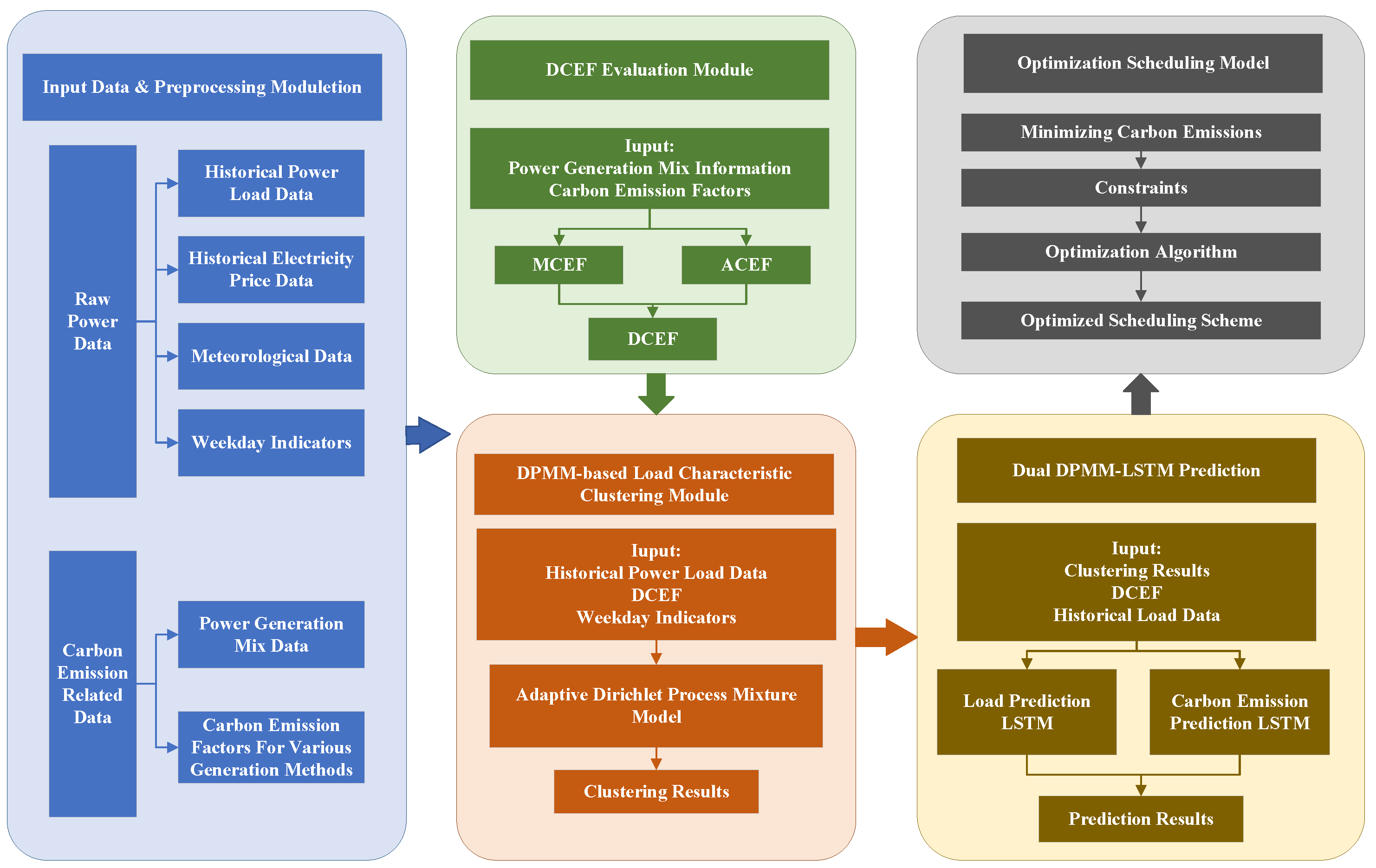
The framework diagram of this article is shown in Figure 1. The framework diagram mainly includes five parts: the first is data collection and processing, the second is DCEF assessment, then load characteristic clustering and collaborative prediction, and finally low-carbon target optimization scheduling.

2. Dynamic Carbon Emission Factor Calculation

This section introduces the DCEF assessment module shown in Figure 1. This module is the foundation of the entire low-carbon optimization framework. Its core task is to construct a DCEF that accurately reflects the real-time carbon intensity of the power grid through the innovative integration of MCEF and ACEF.

The power system’s carbon emission characteristics are highly dynamic and complex, making traditional static calculation methods inadequate for capturing real-time emission variations. When determining the DCEF, neither the MCEF nor the ACEF alone suffices:

• ACEF represents the system-wide average emission level but fails to quantify the marginal impact of load changes.
• MCEF reflects instantaneous load-change effects but exaggerates local fluctuations.

To address this, we propose a weighted fusion of MCEF and ACEF for DCEF calculation. This hybrid approach preserves baseline emission levels while accurately characterizing load-induced marginal effects.

2.1. Marginal Carbon Emission Factors

We assume that the carbon emissions of a power plant are determined by the carbon emission intensity of the fuel and the power generation efficiency. The unit carbon emissions of power plant p using a specific fuel f are given by the following formula:

$$\begin{array}{c}\hfill c_p={\displaystyle \frac{c_f}{{\mu }_p^f}},\end{array}$$

(1)

where $c_f$ is the carbon emission intensity of some fuel f and ${\mu }_p^f$ is the efficiency of power generation at power plant p for fuel f. Formula (1) reflects the energy conversion relationship in the power generation process. The higher the efficiency, the lower the carbon emissions per power generation unit.

In order to accurately assess the actual impact of changes in power demand on system carbon emissions, it is necessary to introduce MCEF. The MCEF represents the additional carbon emissions caused by an increase in power demand by one unit. Considering the power system at time t, the MCEF is defined as

$$\begin{array}{c}\hfill \mathrm{MCEF}\left(t\right)={\displaystyle \frac{\mathrm{\Delta }{E}_M\left(t\right)}{\mathrm{\Delta }{D}_M\left(t\right)}},\end{array}$$

(2)

where $\mathrm{\Delta }{E}_M\left(t\right)$ is the incremental carbon emission of the marginal system at time t and $\mathrm{\Delta }{D}_M\left(t\right)$ is the incremental power demand of the marginal system at time t.

According to Formula (1), the MCEF can be further expressed as

$$\begin{array}{c}\hfill \mathrm{MCEF}\left(t\right)={\displaystyle \frac{{\sum }_{p\in P}{c}_p{\sigma }_p^M\left(t\right)}{\eta }},\end{array}$$

(3)

where $0<\eta \le 1$ is power transmission efficiency, $p\in \{1,2,\dots ,P\}$, and ${\sigma }_p^M\left(t\right)$ is a binary variable indicating whether the generator unit participates in marginal power generation. ${\sigma }_p^M\left(t\right)$ can be written as

$$\begin{array}{c}\hfill {\sigma }_p^M\left(t\right)=\left\{\begin{array}{cc}1,& \mathrm{if}\sum _{i=1}^{p-1}{P}_i^{\mathrm{inst}}<P_{\mathrm{resi}}\left(t\right)\le \sum _{i=1}^p{P}_i^{\mathrm{inst}}\\ 0,& \mathrm{else}\end{array}\right.\end{array}$$

where $P_{\mathrm{resi}}\left(t\right)$ is the residual power load at time t and $P_i^{\mathrm{inst}}$ is the installed capacity of the generator set.

The MCEF reflects the change in carbon emissions caused by the load increment. In the power system, the marginal units in different periods are often different, which results in the dynamic change in the MCEF over time.

2.2. Average Carbon Emission Factors

Unlike the MCEF, which reflects the carbon emission intensity of the incremental load of the power system, the ACEF reflects the overall carbon emission level of the power system over some time.

The ACEF is defined as

$$\begin{array}{c}\hfill \mathrm{ACEF}\left(t\right)={\displaystyle \frac{E_A\left(t\right)}{D_A\left(t\right)}},\end{array}$$

(4)

where $E_A\left(t\right)$ is the total carbon emissions of the system at time t and $D_A\left(t\right)$ is the total power consumption of the system at time t.

For the pth power plant, its carbon emissions $E_p\left(t\right)$ can be expressed as

$$\begin{array}{c}\hfill E_p\left(t\right)=c_p{\sigma }_p^A\left(t\right)P_p^{\mathrm{inst}},\end{array}$$

(5)

where $c_p$ is the carbon emission intensity of power plant p and $P_p^{\mathrm{inst}}$ is its installed capacity. ${\sigma }_p^A\left(t\right)$ is the capacity utilization coefficient, which can be expressed as

$$\begin{array}{c}\hfill {\sigma }_p^A\left(t\right)=\left\{\begin{array}{cc}1,& \mathrm{if}\sum _{i=1}^p{P}_i^{\mathrm{inst}}<P_{\mathrm{resi}}\left(t\right),\\ 0,& \mathrm{if}\sum _{i=1}^{p-1}{P}_i^{\mathrm{inst}}\ge P_{\mathrm{resi}}\left(t\right),\\ {\displaystyle \frac{P_{\mathrm{resi}}\left(t\right)-{\sum }_{i=1}^{p-1}{P}_i^{\mathrm{inst}}}{P_p^{\mathrm{inst}}}},& \mathrm{else}.\end{array}\right.\end{array}$$

where ${\sigma }_p^A\left(t\right)$ is a piecewise function used to determine the capacity utilization of a power plant. When ${\sum }_{i=1}^p{P}_i^{\mathrm{inst}}<P_{\mathrm{resi}}\left(t\right)$, it means that when the cumulative installed capacity is less than the reserved capacity, the power plant operates at full load. When ${\sum }_{i=1}^{p-1}{P}_i^{\mathrm{inst}}\ge P_{\mathrm{resi}}\left(t\right)$, it means that when the previous cumulative installed capacity has reached or exceeded the reserved capacity, the power plant stops operating. In other cases, it indicates partial load operation, which is operated according to the ratio of remaining demand to installed capacity.

We sum the emissions of all power plants in the system to obtain the total carbon emissions of the system

$$\begin{array}{c}\hfill E_A\left(t\right)=\sum _{p\in P}{E}_p\left(t\right).\end{array}$$

Next, we need to calculate the actual power consumption $D_A\left(t\right)$ of the system. The total power generated by the power generation side can be expressed as

$$\begin{array}{c}\hfill D_F^g\left(t\right)=\sum _{f\in F}{D}_f^g\left(t\right),\end{array}$$

where $D_f^g\left(t\right)$ is the amount of power generated by each fuel type f at time t and F is the set of all fuel types for power generation.

Taking into account the loss during transmission, the amount of power reaching the user side is

$$\begin{array}{c}\hfill D_A\left(t\right)=\eta D_F^g\left(t\right),\end{array}$$

where $0<\eta \le 1$ is power transmission efficiency.

According to Formula (4), one can get

$$\begin{array}{c}\hfill \mathrm{ACEF}\left(t\right)={\displaystyle \frac{{\sum }_{p\in P}{c}_p{\sigma }_p^A\left(t\right)P_p^{\mathrm{inst}}}{\eta {\sum }_{f\in F}{D}_f^g\left(t\right)}}.\end{array}$$

(6)

2.3. Dynamic Carbon Emission Factors

By introducing the weight coefficient $\alpha \left(t\right)$, MCEF and ACEF are weighted to calculate DCEF

$$\begin{array}{c}\hfill \mathrm{DCEF}\left(t\right)=\alpha \left(t\right)\mathrm{ACEF}\left(t\right)+(1-\alpha (t\left)\right)\mathrm{MCEF}\left(t\right),\end{array}$$

(7)

where $0\le \alpha \left(t\right)\le 1$. The calculation formula for the time-varying weight coefficient $\alpha \left(t\right)$ is

$$\begin{array}{c}\hfill \alpha \left(t\right)=1-{\displaystyle \frac{P\left(t\right)-P(t-1)}{\mathrm{\Delta }{P}_{max}}},\end{array}$$

(8)

where $P\left(t\right)-P(t-1)$ indicates the load change rate at the current instants. $\mathrm{\Delta }{P}_{max}$ is the maximum load change observed in history.

Remark 1.

The proposed DCEF is derived from a weighted MCEF-ACEF fusion and is positioned as a more robust evaluation method than traditional static methods. Traditional static CEFs [10,11,12] cannot track real-time operational dynamics or marginal generation impacts. The MCEF methods [15] are sensitive to system noise and tend to overestimate the impact of demand response. The ACEF methods [13], although stable, are slow to respond to the key marginal effects that guide real-time optimization. Our DCEF model overcomes this contradiction through a dynamic weight $\alpha \left(t\right)$. The carbon signal it generates can respond sensitively to marginal changes and has good resilience to noise, thus providing a more accurate and robust basis for designing effective low-carbon demand response strategies.

3. Power Consumption and DCEF Clustering and Prediction Model

This section corresponds to the DPMM load characteristic clustering module and the dual DPMM-LSTM prediction module in Figure 1. This module aims to first adaptively identify potential patterns in electricity consumption and carbon emission data through a data-driven approach. Then, based on these pattern characteristics, it accurately and collaboratively predicts electricity consumption and DCEF for the next 24 h, providing key input for subsequent optimized scheduling.

3.1. Dirichlet Process Mixture Model Principle

The DPMM [34] is a non-parametric Bayesian clustering approach that automatically infers the number of clusters. It models data as a mixture of an unknown number of distributions, with each observation generated from a distribution whose parameters are governed by a Dirichlet process.

We assume that the observed data point $x_i$ is generated from a distribution with parameters ${\theta }_i$:

$$\begin{array}{cc}\hfill & x_i|{\theta }_i\sim p\left(x_i\right|{\theta }_i),\hfill \\ \hfill & {\theta }_i|G\sim G,\hfill \end{array}$$

where $p(·)$ represents the probability density function. The random distribution G follows a Dirichlet process

$$\begin{array}{c}\hfill G|\alpha ,G_0\sim DP(\alpha ,G_0),\end{array}$$

where $\alpha$ is the concentration parameter, which controls the probability of generating new categories; $G_0$ is the reference distribution, which determines the parameter distribution of the newly generated categories.

In order to better understand the data generation process, the hidden variable $z_i$ is introduced to represent the category to which each data point belongs. The model can be rewritten as

$$\begin{array}{c}\hfill z_i|\pi \sim \mathrm{Multinomial}\left(\pi \right),\\ \hfill x_i|z_i,\theta \sim p\left(x_i\right|{\theta }_{z_i}),\end{array}$$

where $\mathrm{Multinomial}(·)$ is a discrete probability distribution used to describe the probability of selecting multiple categories and $\pi$ represents the probability of selecting each category.

When classifying a new data point, we use the Bayes theorem to calculate the posterior probability. According to the Bayes theorem, the posterior probability is proportional to the product of the prior probability and the likelihood function:

$$\begin{array}{c}\hfill p\left(z_i\right|z_{-i},x_i,\theta )\propto p\left(z_i\right|z_{-i})p\left(x_i\right|{\theta }_{z_i}).\end{array}$$

Next, we can obtain the specific probability of a new data point being assigned to each category

$$\begin{array}{cc}\hfill p& (z_i=k\mid z_{-i},x_i,\theta )\hfill \\ \hfill & \propto \left\{\begin{array}{cc}{n}_k·p(x_i\mid {\theta }_k),\hfill & \mathrm{Existing}\mathrm{Categories}\hfill \\ \alpha \int p(x_i\mid \theta )d{G}_0\left(\theta \right),\hfill & \mathrm{New}\mathrm{Category}\hfill \end{array}\right.\hfill \end{array}$$

where $n_k$ is the number of existing data points in category k. This result shows that data points may either join existing categories or create new categories, which is determined by the characteristics of the data itself and the existing category structure.

To implement this category assignment mechanism, we must compute each data point’s probability of belonging to each category. This requires defining an observation model describing the data distribution per category. Given that real-world data often follow approximately normal distributions and for computational convenience, we typically use a Gaussian distribution as our observation model

$$\begin{array}{c}\hfill x_i|{\mu }_k,{\mathrm{\Sigma }}_k\sim \mathcal{N}({\mu }_k,{\mathrm{\Sigma }}_k),\end{array}$$

where ${\mu }_k$ and ${\mathrm{\Sigma }}_k$ are the mean vector and the covariance matrix of the kth category. $\mathcal{N}(·)$ represents a multi-dimensional gaussian distribution. The corresponding conjugate prior distribution is

$$\begin{array}{c}\hfill {\mu }_k|{\mathrm{\Sigma }}_k\sim \mathcal{N}({\mu }_0,{\mathrm{\Sigma }}_k/{\kappa }_0),\\ \hfill {\mathrm{\Sigma }}_k\sim \mathcal{IW}({\nu }_0,{\mathrm{\Psi }}_0),\end{array}$$

where $\mathcal{IW}(·)$ is the inverse Wishart distribution. Hyperparameters ${\mu }_0$, ${\kappa }_0>0$, ${\nu }_0>d-1$, and ${\mathrm{\Psi }}_0>0$ need to be set before the algorithm starts and their choice affects the behavior of the model.

For a new data point, its predicted distribution can be expressed as

$$\begin{array}{cc}\hfill p\left(x_{new}\right|x_{1:n})=& \sum _{k=1}^K{\displaystyle \frac{n_k}{n+\alpha }}p\left(x_{new}\right|{\widehat{\theta }}_k)\hfill \\ \hfill & +{\displaystyle \frac{\alpha }{n+\alpha }}\mathit{\int }p\left(x_{new}\right|\theta )d{G}_0\left(\theta \right),\hfill \end{array}$$

where ${\widehat{\theta }}_k$ is the estimated parameter of the kth existing category.

DPMM not only considers existing categories but also reserves the possibility of generating new categories, which enables the model to adjust the number of categories as the data increase naturally.

3.2. LSTM Network Principle

LSTM [20] is a specialized recurrent neural network featuring a cell state that propagates information throughout the network via gating mechanisms. Its architecture comprises three gates (forget, input, output) and a memory unit.

The forget gate determines the extent to which the information in the cell state at the previous moment needs to be retained or discarded. Its expression is as follows:

$$\begin{array}{c}\hfill f\left(t\right)=\sigma (W_f·[h(t-1),x\left(t\right)]+b_f),\end{array}$$

where $\sigma$ represents the sigmoid activation function, $W_f$ is the weight matrix, $h(t-1)$ is the hidden state of the previous moment, $x\left(t\right)$ is the current input, and $b_f$ is the bias term. The output of the forget gate is a value between 0 and 1, where 1 means completely retained and 0 means completely discarded.

The input gate controls the extent to which new information enters the cell state and consists of two parts: the input gate vector $i\left(t\right)$ and the candidate memory cell $\tilde{C}\left(t\right)$

$$\begin{array}{cc}\hfill & i\left(t\right)=\sigma (W_i·[h(t-1),x\left(t\right)]+b_i),\hfill \\ \hfill & \tilde{C}\left(t\right)=tanh(W_C·[h(t-1),x\left(t\right)]+b_c),\hfill \end{array}$$

where $W_i$, $W_C$, $b_i$ and $b_c$ are the weight matrix and bias of the input gate and candidate memory respectively, and $tanh(·)$ is the hyperbolic tangent activation function, which limits the output to $[-1,1]$.

The new cell state is updated as follows:

$$\begin{array}{c}\hfill C\left(t\right)=f\left(t\right)\odot C(t-1)+i\left(t\right)\odot \tilde{C}\left(t\right),\end{array}$$

where $C\left(t\right)$ and $C(t-1)$ are the cell state at the current time step and the cell state at the previous time step, respectively. ⊙ represents the element-by-element multiplication.

The output gate regulates the extent to which the cell state information is propagated to the hidden state, as expressed by the following equation:

$$\begin{array}{cc}\hfill & o\left(t\right)=\sigma (W_o·[h(t-1),x\left(t\right)]+b_o),\hfill \\ \hfill & h\left(t\right)=o\left(t\right)\odot tanh\left(C\right(t\left)\right),\hfill \end{array}$$

where $o\left(t\right)$ is the activation value of the output gate, $h\left(t\right)$ is the hidden state of the current time step, $W_o$ and $b_o$ are the weight matrix and bias of the output gate, respectively.

3.3. Clustering and Prediction Model Design

We assume that the calculated hourly DCEF data set is $\mathrm{DCEF}=\{dce{f}_1,dce{f}_2,\dots ,dce{f}_n\}$ and the power consumption data $\mathrm{PC}=\{p{c}_1,p{c}_2,\dots ,p{c}_n\}$, where n is the number of samples.

This paper uses the DPMM model for cluster analysis, which can be expressed as

$$\begin{array}{cc}\hfill & G\sim DP(\alpha ,G_0),\hfill \\ \hfill & {\theta }_i\sim G,\hfill \\ \hfill & x_i\sim F\left({\theta }_i\right),\hfill \end{array}$$

where G is the random probability measure, $DP(\alpha ,G_0)$ represents the Dirichlet process, $\alpha$ is the concentration parameter, and $G_0$ is the benchmark measure. ${\theta }_i$ represents the parameter of the ith observation data, and $F\left({\theta }_i\right)$ is the likelihood function of the observation data.

For DCEF data, the generation process can be described as

$$\begin{array}{c}\hfill \mathrm{DCEF}\sim \sum _{i=1}^n{\pi }_{i}N({\mu }_i,{\mathrm{\Sigma }}_i),\end{array}$$

where ${\pi }_i$ is the mixing weight satisfying ${\sum }_{i=1}^n{\pi }_i=1$. $N({\mu }_i,{\mathrm{\Sigma }}_i)$ represents Gaussian distribution, ${\mu }_i$ and ${\mathrm{\Sigma }}_i$ are the mean and covariance matrix of the ith component, respectively.

Similarly, the generation process of power consumption data can be expressed as

$$\begin{array}{c}\hfill \mathrm{PC}\sim \sum _{j=1}^n{\omega }_{j}N({\upsilon }_j,{\mathrm{\Lambda }}_j),\end{array}$$

where ${\omega }_j$ is the mixing weight. ${\upsilon }_j$ and ${\mathrm{\Lambda }}_j$ are the mean and covariance matrix of the jth component, respectively.

The posterior distribution of the DPMM model can be inferred by Gibbs sampling

$$\begin{array}{c}\hfill P\left({\theta }_i\right|{\theta }_{-i},x_{1:n})\propto f\left(x_i\right|{\theta }_i)\times (\alpha \times P\left({\theta }_i\right|G_0)+\sum _{j\ne i}\delta \left({\theta }_j\right)),\end{array}$$

where ${\theta }_{-i}$ represents all parameters except ${\theta }_i$, $f\left(x_i\right|{\theta }_i)$ is the likelihood function, and $\delta \left({\theta }_j\right)$ is the Dirac function.

Through this model, we can obtain the clustering results of DCEF data ${\mathrm{DCEF}}_{clusters}=\{C{F}_1,C{F}_2,\dots ,C{F}_k\}$ and power consumption data $P{C}_{clusters}=\{P{C}_1,P{C}_2,\dots ,P{C}_m\}$, where k and m are the optimal numbers of clusters determined adaptively.

When constructing the input features of the LSTM prediction model, we first need to determine the feature category of the historical data. These historical data need to be calculated separately from the feature class center obtained by DPMM clustering to determine the feature category to which they belong.

For DCEF data, assuming that DPMM clustering obtains k feature class centers $C=\{c_1,c_2,\dots ,c_k\}$, the distance between the carbon emission factor data at each time t and the ith class center can be expressed as

$$\begin{array}{c}\hfill d_{dcef}(t,i)=\parallel dce{f}_t-c_i\parallel ,\end{array}$$

(9)

where $dce{f}_t$ is the CEF data at time t. For the DCEF data at time t, the characteristic category to which it belongs can be determined by the following method:

$$\begin{array}{c}\hfill {\mathrm{class}}_{dcef}\left(t\right)=\underset{i\in [1,k]}{\mathrm{argmin}}{d}_{dcef}(t,i).\end{array}$$

(10)

Similarly, for power consumption data, assuming that DPMM clustering obtains m feature class centers $P=\{p_1,p_2,\dots ,p_m\}$, the distance between the power consumption data at each time t and the jth class center is

$$\begin{array}{c}\hfill d_{pc}(t,j)=\parallel p{c}_t-p_j\parallel .\end{array}$$

(11)

The corresponding feature category is determined as

$$\begin{array}{c}\hfill {\mathrm{class}}_{pc}\left(t\right)=\underset{j\in [1,m]}{\mathrm{argmin}}{d}_{pc}(t,j).\end{array}$$

(12)

Through the above calculation, we can deetrmine the feature category of the historical data at each moment. When constructing the input of the LSTM prediction model, this feature category information is fused with the original data. For the LSTM model for DCEF prediction, the input feature vector can be expressed as

$$\begin{array}{c}\hfill X_{dcef}\left(t\right)=[dce{f}_t,{\mathrm{class}}_{dcef}\left(t\right)].\end{array}$$

(13)

Similarly, the input feature vector of the LSTM model for power consumption prediction is

$$\begin{array}{c}\hfill X_{pc}\left(t\right)=[p{c}_t,{\mathrm{class}}_{pc}\left(t\right)].\end{array}$$

(14)

We employ a three-layer LSTM architecture with 128, 64, and 32 units per layer for hierarchical feature extraction, fusion, and abstraction. Input data are standardized and preprocessed, with training samples generated via sliding time windows to enhance model performance.

Through the above model, the predicted dynamic carbon emission factor data and power consumption data are obtained, which is convenient for subsequent low-carbon scheduling research.

Remark 2.

By combining the original data with the feature category information to which it belongs, the LSTM model [20,21] can simultaneously learn the temporal change characteristics and clustering characteristics of the data. Feature category information, as a high-level semantic feature, helps the model capture the periodic patterns and typical change laws of the data. For example, the carbon emission factor in certain periods may belong to the low-carbon feature class, while the power consumption may belong to the high-load feature class. This feature combination information is significant for the prediction model in understanding the system operation status.

Remark 3.

Our framework combines adaptive DPMM clustering with dual LSTM architecture to overcome limitations in low-carbon demand forecasting. Unlike standard LSTM models [20,21] that fail to distinguish operational patterns (weekdays/holidays, seasons) or traditional clustering [22,23,24] requiring preset cluster numbers, our DPMM automatically identifies optimal operational modes. These pattern features, combined with historical data, feed into a dual LSTM network for coordinated prediction of both key variables.

4. Low-Carbon Demand Response Optimization Model

Based on the prediction results from the previous stage, this section elaborates on the optimized scheduling model shown in Figure 1. This model focuses on maximizing carbon emission reductions and comprehensively considers multiple constraints, such as system security, equipment limitations, and user comfort, ultimately generating an optimal load adjustment plan.

4.1. Objective Function

We assume that the DCEF data and power consumption data for the next 24 h obtained by the DPMM-LSTM algorithm are communicated to the user in advance. The user can maximize its carbon emission reduction by adjusting its electricity consumption behavior in the next 24 h.

The expression of the objective function is

$$\begin{array}{c}\hfill max\sum _{t\in T}\mathrm{\Delta }{\mathrm{PC}}^{-}\left(t\right)\mathrm{DCEF}\left(t\right)-\mathrm{\Delta }{\mathrm{PC}}^{+}\left(t\right)\mathrm{DCEF}\left(t\right),\end{array}$$

(15)

where $T=\{1,2,\dots ,T\}$, $\mathrm{\Delta }{\mathrm{PC}}^{+}\left(t\right)$ represents the increase in power consumption at time t, and $\mathrm{\Delta }{\mathrm{PC}}^{-}\left(t\right)$ represents the decrease in power consumption at time t. The objective Function (15) achieves the greatest possible reduction in system carbon emissions by shifting power load from high-carbon emission periods to low-carbon emission periods.

4.2. Constraint Design

This paper establishes a comprehensive constraint system with rigid and flexible categories to ensure optimization feasibility. Rigid constraints (daily power conservation and power limits) guarantee system safety and equipment reliability, while flexible constraints (load change rates and user comfort) address operational stability and user experience.

We consider the following rigid constraints.

(1) Daily power conservation constraints: this constraint ensures that the total power consumption before and after demand response adjustment remains unchanged, and the expression is

$$\begin{array}{c}\hfill \sum _{t\in T}\mathrm{\Delta }{\mathrm{PC}}^{+}\left(t\right)-\mathrm{\Delta }{\mathrm{PC}}^{-}\left(t\right)=0.\end{array}$$

(16)

Constraint (16) ensures that demand response adjusts only the power consumption sequence while preserving total energy demand.

(2) Power limit constraints: this constraint requires that the actual load in each time period must be controlled within the range allowed by the system, which can be expressed as

$$\begin{array}{cc}\hfill & P_0\left(t\right)+\mathrm{\Delta }{\mathrm{PC}}^{+}\left(t\right)-\mathrm{\Delta }{\mathrm{PC}}^{-}\left(t\right)\le P_{max}\hfill \end{array}$$

(17)

$$\begin{array}{cc}\hfill & P_0\left(t\right)+\mathrm{\Delta }{\mathrm{PC}}^{+}\left(t\right)-\mathrm{\Delta }{\mathrm{PC}}^{-}\left(t\right)\ge P_{min}\hfill \end{array}$$

(18)

where $P_0\left(t\right)$ is the reference load, $P_{max}$ and $P_{min}$ are the maximum and minimum loads allowed by the system, respectively. Constraints (17) and (18) ensure system safety by limiting load adjustments to avoid overload or instability.

We consider the following flexible constraints.

(3) Load change rate constraints: this constraint limits the load change rate between adjacent time periods, which is

$$\begin{array}{cc}\hfill & \parallel (\mathrm{\Delta }{\mathrm{PC}}^{+}\left(t\right)-\mathrm{\Delta }{\mathrm{PC}}^{-}\left(t\right))\hfill \\ \hfill & -(\mathrm{\Delta }{\mathrm{PC}}^{+}(t-1)-\mathrm{\Delta }{\mathrm{PC}}^{-}(t-1))\parallel \le R_r,\hfill \end{array}$$

(19)

where $R_r>0$ is the maximum load change rate allowed. Constraint (19) helps to avoid the impact of severe load fluctuations on the power grid and reduce the power grid fluctuations caused by rapid load changes.

(4) User comfort constraints: this constraint controls the impact of load adjustment on the daily life and production activities of the user, which can be written as

$$\begin{array}{c}\hfill \parallel \mathrm{\Delta }{\mathrm{PC}}^{+}\left(t\right)-\mathrm{\Delta }{\mathrm{PC}}^{-}\left(t\right)\parallel \le \beta P_0\left(t\right),\end{array}$$

(20)

where $\beta$ is the load adjustment ratio coefficient acceptable to the user. Constraint (20) ensures that the load adjustment is within the acceptable range for the user. Different types of users can set different $\beta$ values according to their power consumption characteristics to better meet the actual needs of various users.

Remark 4.

Unlike conventional demand response programs that primarily target economic benefits by responding to price signals [7,8,9], our approach directly optimizes for maximal carbon reduction by leveraging the real-time carbon intensity information embedded in the DCEF. This allows Optimization (15) to identify and exploit true low-carbon periods for load shifting, ensuring that the demand response actions are precisely guided by their carbon emissions.

4.3. Optimization Problem Solving

This paper uses the sequential quadratic programming method [35] to solve this carbon reduction optimization problem. The core idea of this method is to perform a quadratic approximation on the original nonlinear optimization problem near the current iteration point, transform the nonlinear programming problem into a sequence of quadratic programming subproblems, and then gradually solve these subproblems to obtain the optimal solution of the original problem.

The solution process involves quadratic approximation of the objective function and linearization of constraints at each iteration, transforming our carbon reduction maximization problem into a linearly constrained quadratic programming (QP) subproblem. Solving this QP yields search direction and step size for solution updates, iterating until convergence. Algorithm 1 gives the specific steps.

Algorithm 1 An Algorithm for Demand Response Optimization

1: Input: Predicted $\mathrm{DCEF}\left(t\right)$ and $\mathrm{PC}\left(t\right)$ (for $t\in T$), Problem Constraints (defined by Equations (15)–(20)), Convergence tolerance $ϵ$.   2: Output: Optimal load adjustments $\mathrm{\Delta }{\mathrm{PC}}^{+\ast }\left(t\right)$, $\mathrm{\Delta }{\mathrm{PC}}^{-\ast }\left(t\right)$ (for $t\in T$).   3: Initialize:   4:    Set iteration counter $t\leftarrow 0$.   5:    Choose an initial guess for the variables $x_0={[\mathrm{\Delta }{\mathrm{PC}}_0^{+}\left(t\right),\mathrm{\Delta }{\mathrm{PC}}_0^{-}\left(t\right)]}_{t\in T}$.   6:    Initialize an approximation $B_0$ for the Hessian matrix of the Lagrangian.   7: repeat   8:     Formulate a QP approximation of the original problem (Objective Equation (15), and constraints Equations (16)–(20) at the current point $x_t$).   9:     Solve the formulated QP subproblem to find a search direction $d_t$. 10:     Perform a line search along the direction $d_t$ to determine an appropriate step size ${\alpha }_t>0$. 11:     Update the current solution: $x_{t+1}\leftarrow x_t+{\alpha }_t{d}_t$. 12:     Update the Hessian approximation $B_t$ to $B_{t+1}$ using information from the current iteration. 13:     Increment iteration counter: $t\leftarrow t+1$. 14: until a convergence criterion is met 15: Set the optimal solution $x^{*}\leftarrow x_t$. 16: return $x^{*}={[\mathrm{\Delta }P{C}^{+\ast }\left(t\right),\mathrm{\Delta }P{C}^{-\ast }\left(t\right)]}_{t\in T}$.

5. Case Analysis

In this section, we use a specific case analysis to illustrate the rationality and practicality of the optimal scheduling method for low-carbon demand response resources proposed in this paper.

5.1. Data Collection and Preprocessing

Before conducting case analysis, detailed data collection and processing is required. This study selected various power data from Germany in 2023 as the basic data year. We collected detailed information on various types of power generation units in Germany from the ENTSO-E power system database, which can be found at the following website: https://transparency.entsoe.eu/, accessed on 8 September 2025. It includes the installed capacity of each power plant ($P_{inst}$), the power generation efficiency (${\mu }_p^f$) of different fuel types, the carbon emission intensity of each fuel ($c_f$), the hourly power generation data ($D_f^g$), and the hourly residual load data throughout the year ($P_{resi}$).

For the collected data, (1) outlier detection and processing are performed on the original data; (2) missing data are reasonably filled. By calculating and analyzing Germany’s circuit data for the whole year of 2018, we established a carbon emission assessment system based on the DPMM-LSTM algorithm. Based on this, we predicted the DCEFs and power consumption data for each hour on 8 January 2024–14 January 2024.

5.2. Clustering and Prediction Performance

Figure 2 and Figure 3 show the clustering results where the DPMM algorithm adaptively identified 6 power consumption patterns and 5 DCEF patterns. The detailed cluster characteristics for power consumption and DCEF are shown in

Table 1. Summary of Power Consumption Cluster Characteristics.

Cluster	No. of Samples	Percentage (%)	Peak Time	Valley Time	Avg. 95% CI Width
1	2009	22.08	07:00	22:00	0.4052
2	2001	22.00	19:00	10:00	0.4050
3	1478	16.25	13:00	04:00	0.3952
4	1064	11.70	15:00	03:00	0.4253
5	1488	16.36	01:00	16:00	0.3954
6	1057	11.62	03:00	15:00	0.4257

Note: “Avg. 95% CI Width” refers to the average width of the 95% confidence interval across all time steps for the normalized centroid value. A smaller value indicates lower variance and a more consistent pattern within the cluster.

and

Table 2. Summary of DCEF Cluster Characteristics.

Cluster	No. of Samples	Percentage (%)	High-Carbon Time	Low-Carbon Time	Avg. 95% CI Width
1	2169	25.24	18:00	09:00	0.8819
2	1238	14.41	01:00	07:00	0.9045
3	1693	19.70	05:00	22:00	0.9412
4	1544	17.97	22:00	00:00	0.9381
5	1949	22.68	23:00	17:00	1.1108

Note: “Avg. 95% CI Width” refers to the average width of the 95% confidence interval for the normalized centroid value. A smaller value indicates lower variance. The relatively high CI widths here reflect the greater inherent volatility of carbon intensity compared to load.

, respectively.

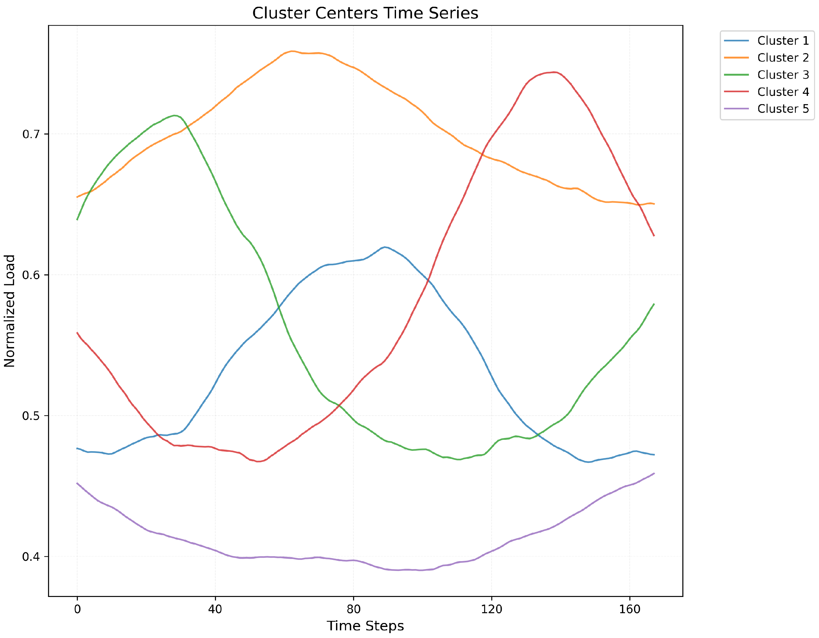
The power consumption data are adaptively clustered into 6 distinct groups, capturing key operational patterns such as high-load profiles during winter (Clusters 4 and 6) and medium-load patterns with varying peaks in summer (Clusters 3 and 5). Similarly, the DCEFs are clustered into 5 groups representing different carbon intensity levels. This analysis reveals distinct temporal and seasonal characteristics, for instance, a low-carbon profile found predominantly in winter (Cluster 5), likely due to high renewable output, and a medium-carbon pattern associated with weekday mornings in summer (Cluster 1). Figure 4 and Figure 5 depict the centroid curves for the power consumption and DCEF clusters, respectively, visualizing these distinct operational patterns.

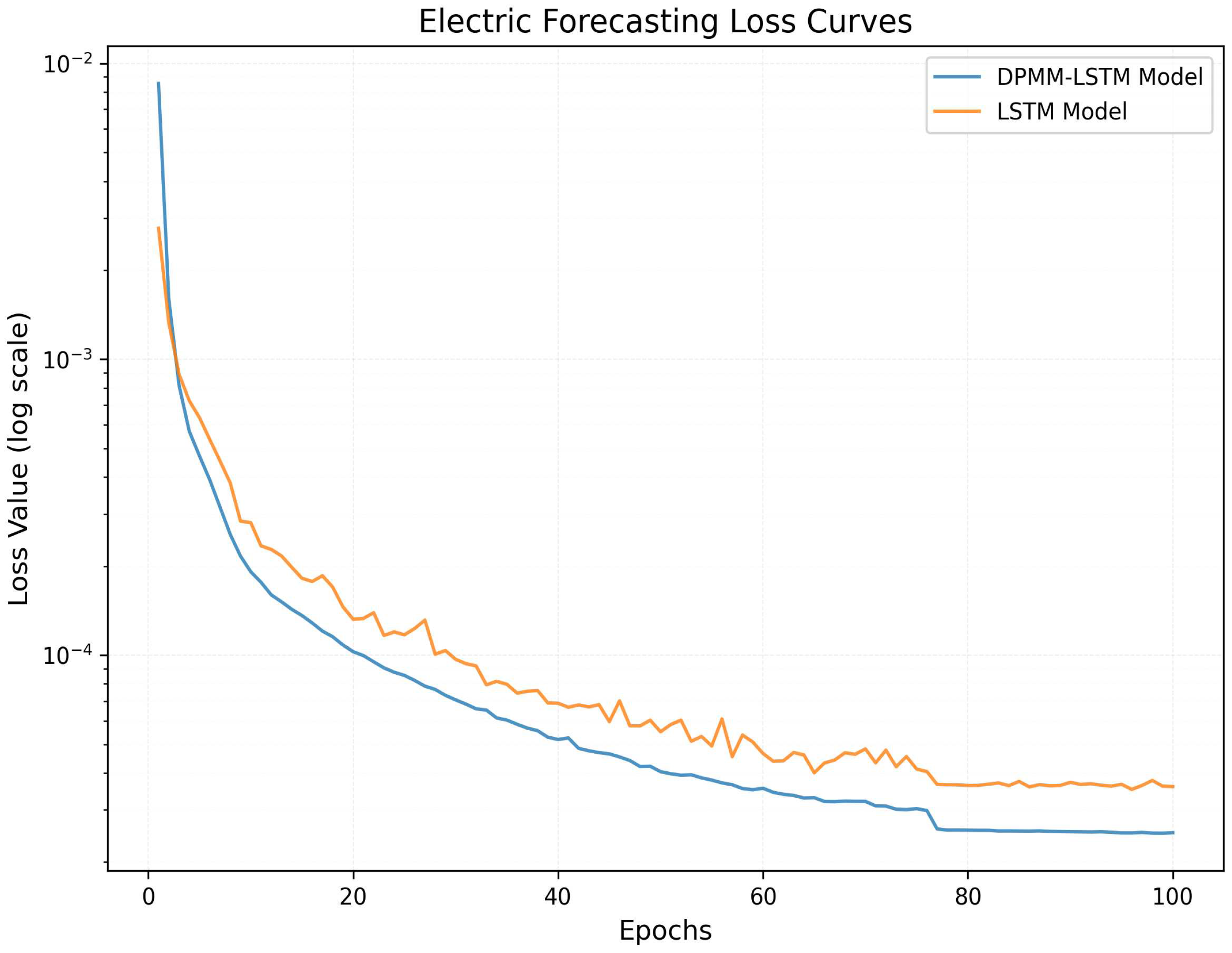
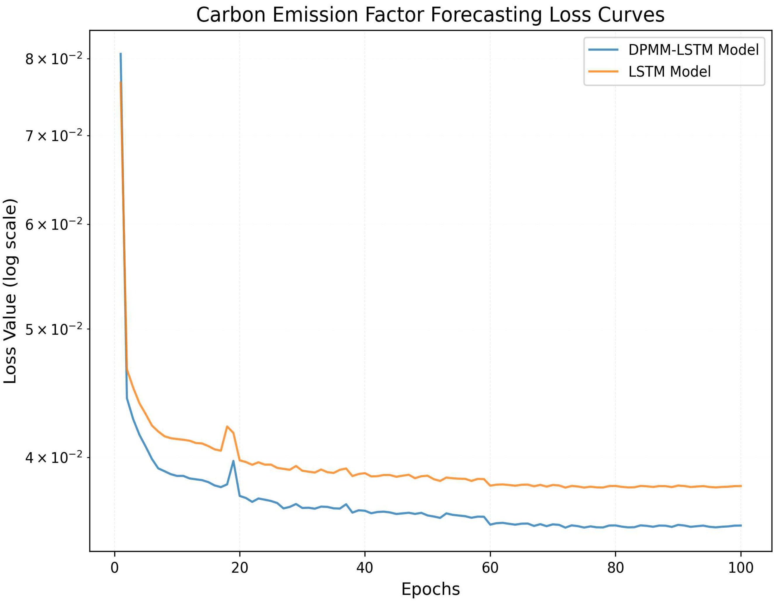
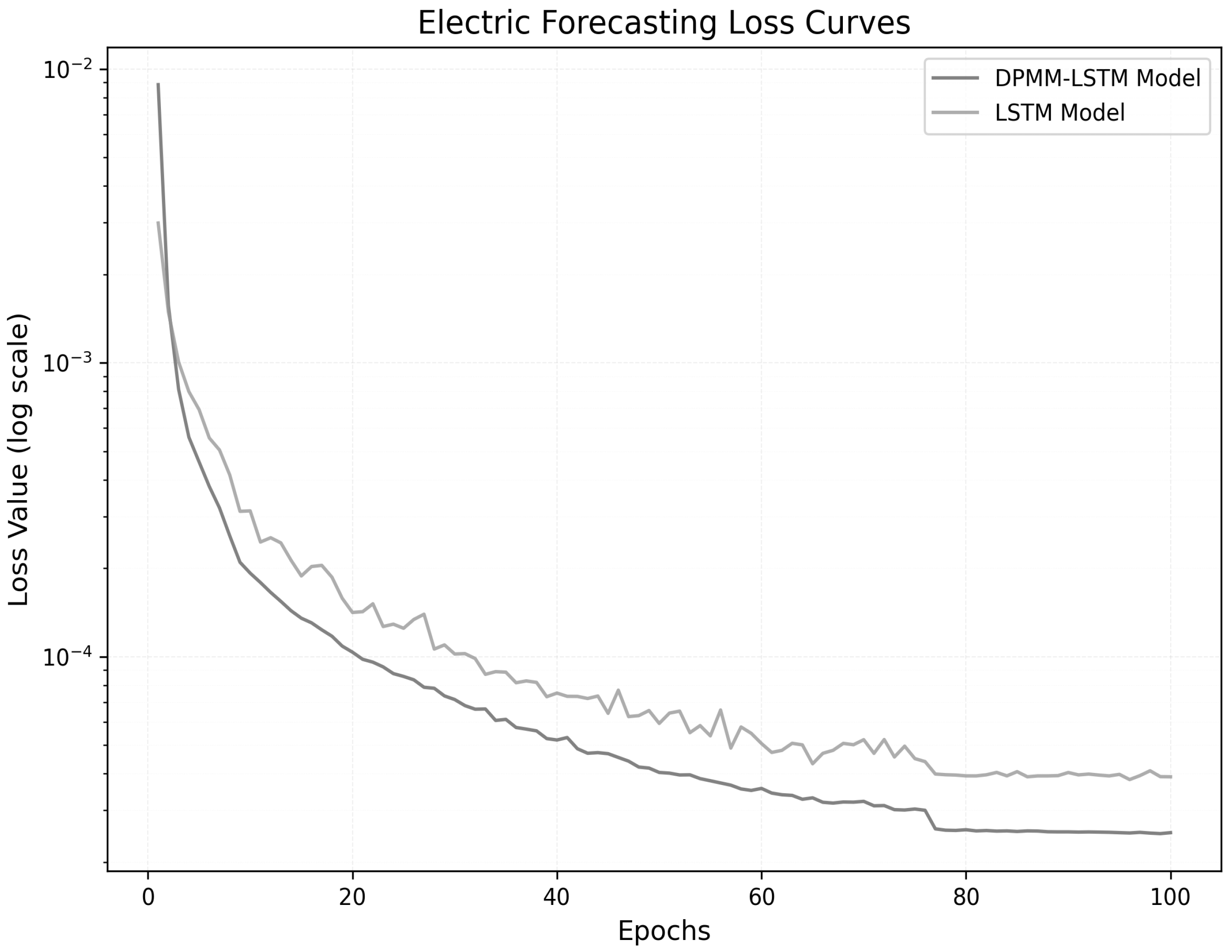
Figure 6 and Figure 7 show the training loss curves for power consumption and CEF prediction, respectively, comparing the performance of the proposed DPMM-LSTM model with a baseline LSTM model. As can be seen from Figure 6 and Figure 7, the loss curve of the DPMM-LSTM model (blue curve) remains lower than that of the baseline LSTM model (orange curve) throughout the training process, indicating that our model achieves a lower final loss value, indicating higher prediction accuracy.

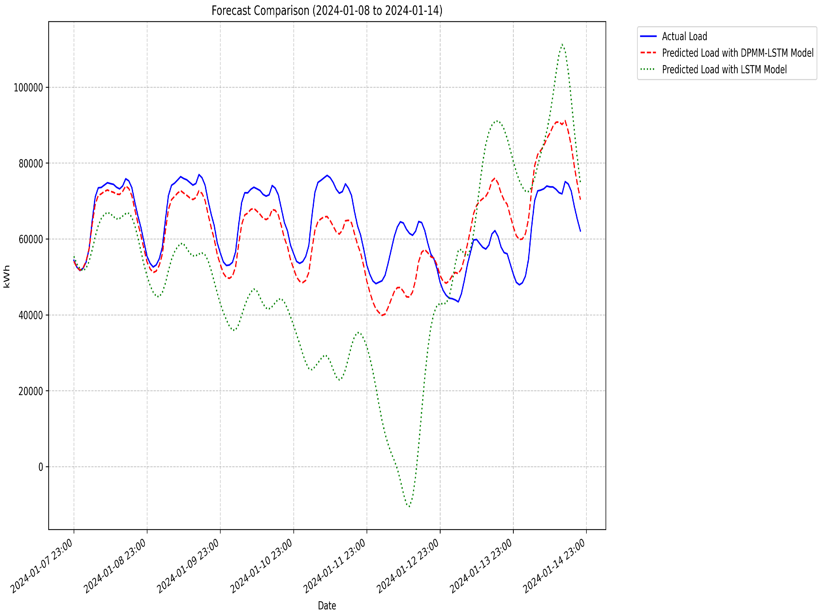
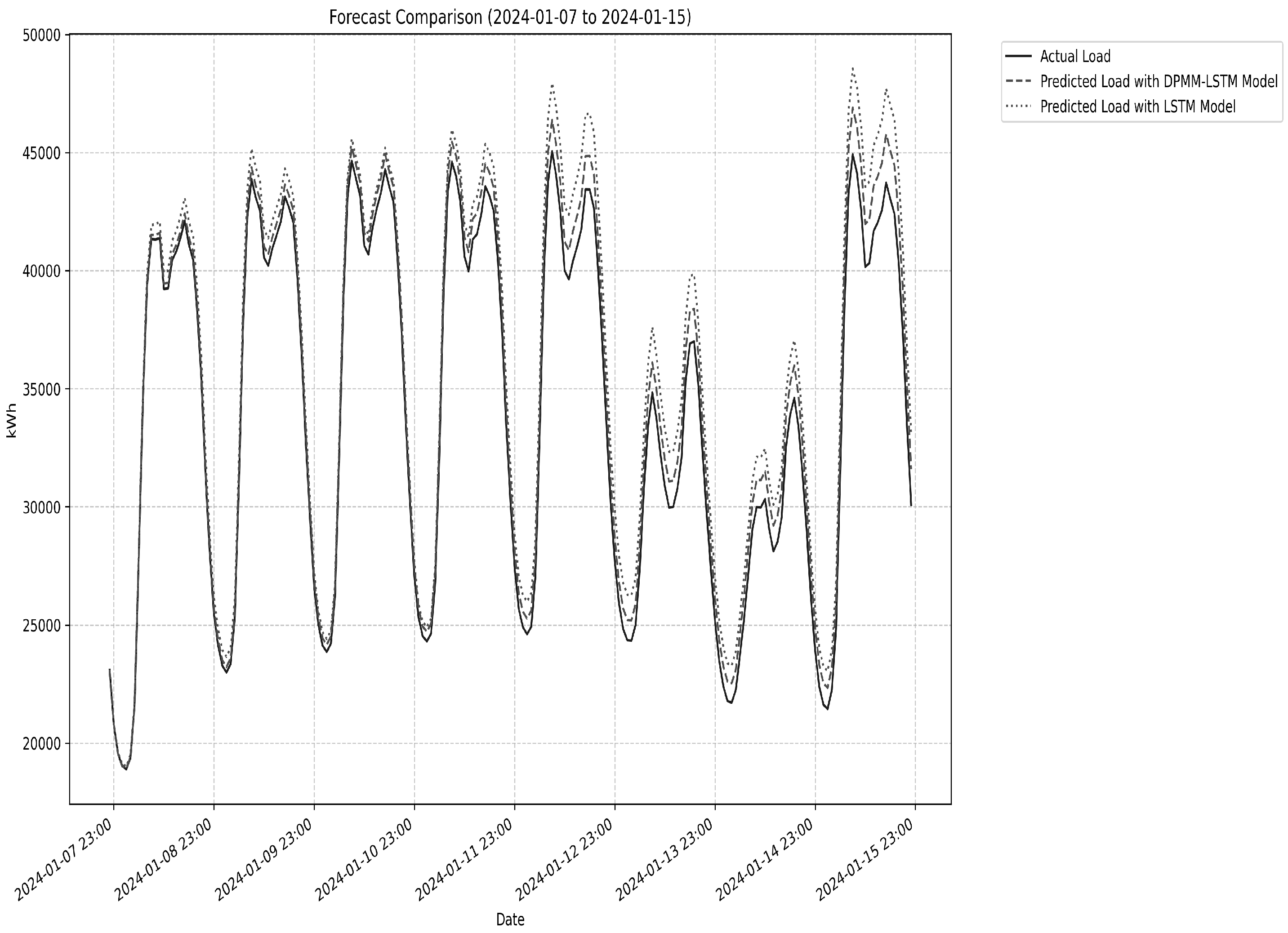
Figure 8 and Figure 9 are the data changes in the predicted DCEFs and power consumption. In Figure 9, the DPMM-LSTM model’s prediction curve (dashed red line) closely matches the actual load curve (solid blue line), accurately capturing the daily peak and valley cycles and amplitude. In contrast, the baseline LSTM model’s prediction (dotted gray line) exhibits systematic deviations. Similarly, in Figure 8, our model demonstrates superior tracking ability, successfully reproducing several key peaks and valleys, while the baseline LSTM model tends to output an overly smooth trend, ignoring these key dynamics that determine marginal effects. These charts strongly demonstrate the effectiveness of our approach.

Table 3. Prediction Model Performance Comparison.

Model	Prediction Target	MAE	RMSE
DPMM-LSTM	Power Consumption	185.5	250.2
DPMM-LSTM	DCEFs	0.015	0.021
LSTM	Power Consumption	240.8	315.6
LSTM	DCEFs	0.025	0.035

presents a quantitative comparison of the forecasting performance between the proposed DPMM-LSTM model and the baseline LSTM model. The evaluation focuses on predicting both power consumption and Dynamic Carbon Emission Factors (DCEFs) over the test period, using Mean Absolute Error (MAE) and Root Mean Squared Error (RMSE) as performance metrics. The results indicate that the DPMM-LSTM model achieves lower error values for both prediction targets compared to the standard LSTM model.

To further validate the generalization and robustness of our proposed framework, we add a case study on the Italian power grid. Italy’s power generation structure and load patterns differ significantly from those of Germany, serving as an effective comparative validation set. Figure 10 and Figure 11 show the training loss curves for power consumption and carbon emission factor prediction on the Italian dataset, respectively. The loss curve of the DPMM-LSTM model remains consistently lower than that of the baseline LSTM model throughout training. The prediction results in Figure 12 and Figure 13 also demonstrate the superiority of our prediction method. In Figure 13, our model accurately fits the actual load curve of the Italian power grid, while the LSTM model performs less well. Similarly, in Figure 12, our model also achieves better predictions than the LSTM model. These results on the Italian dataset strongly demonstrate that our proposed method is not limited to the power grid of a specific country but rather has good cross-regional applicability and can adapt to diverse power grid environments.

5.3. Demand Response Optimization Results

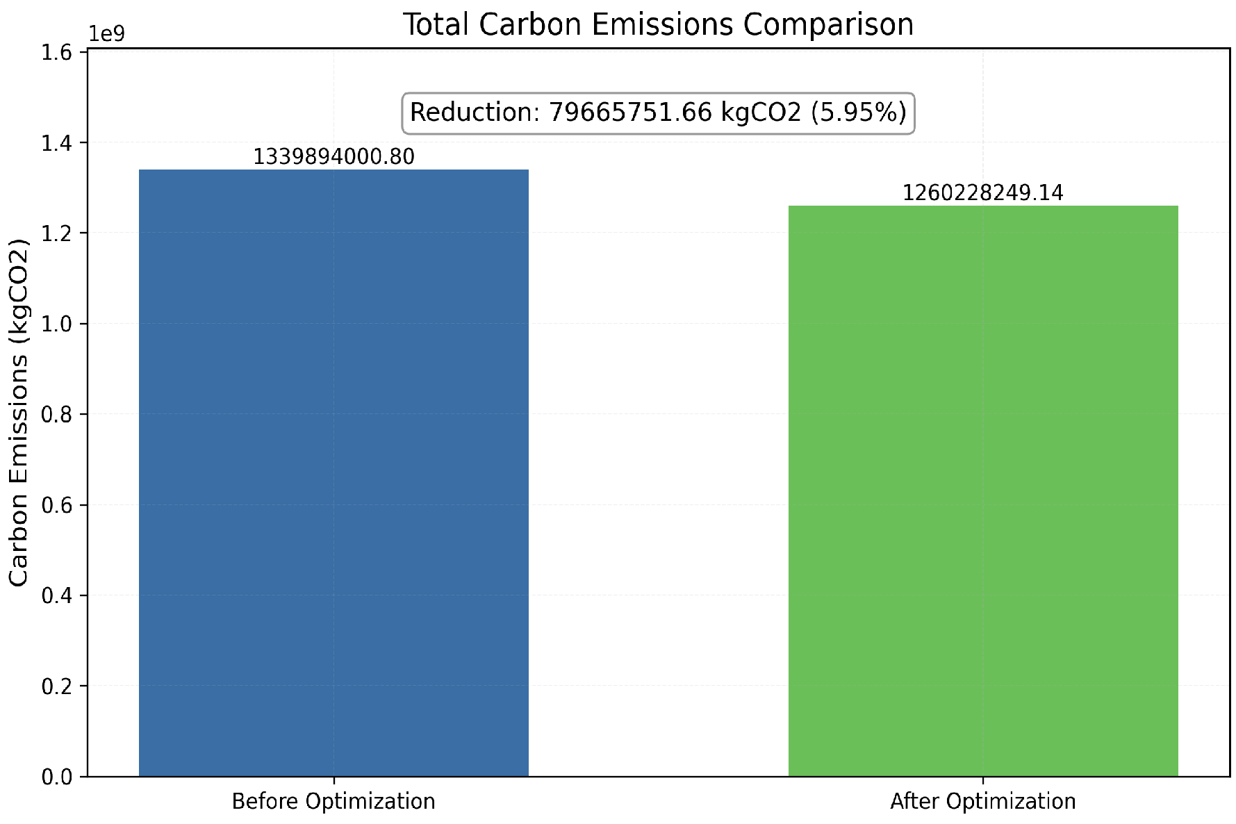
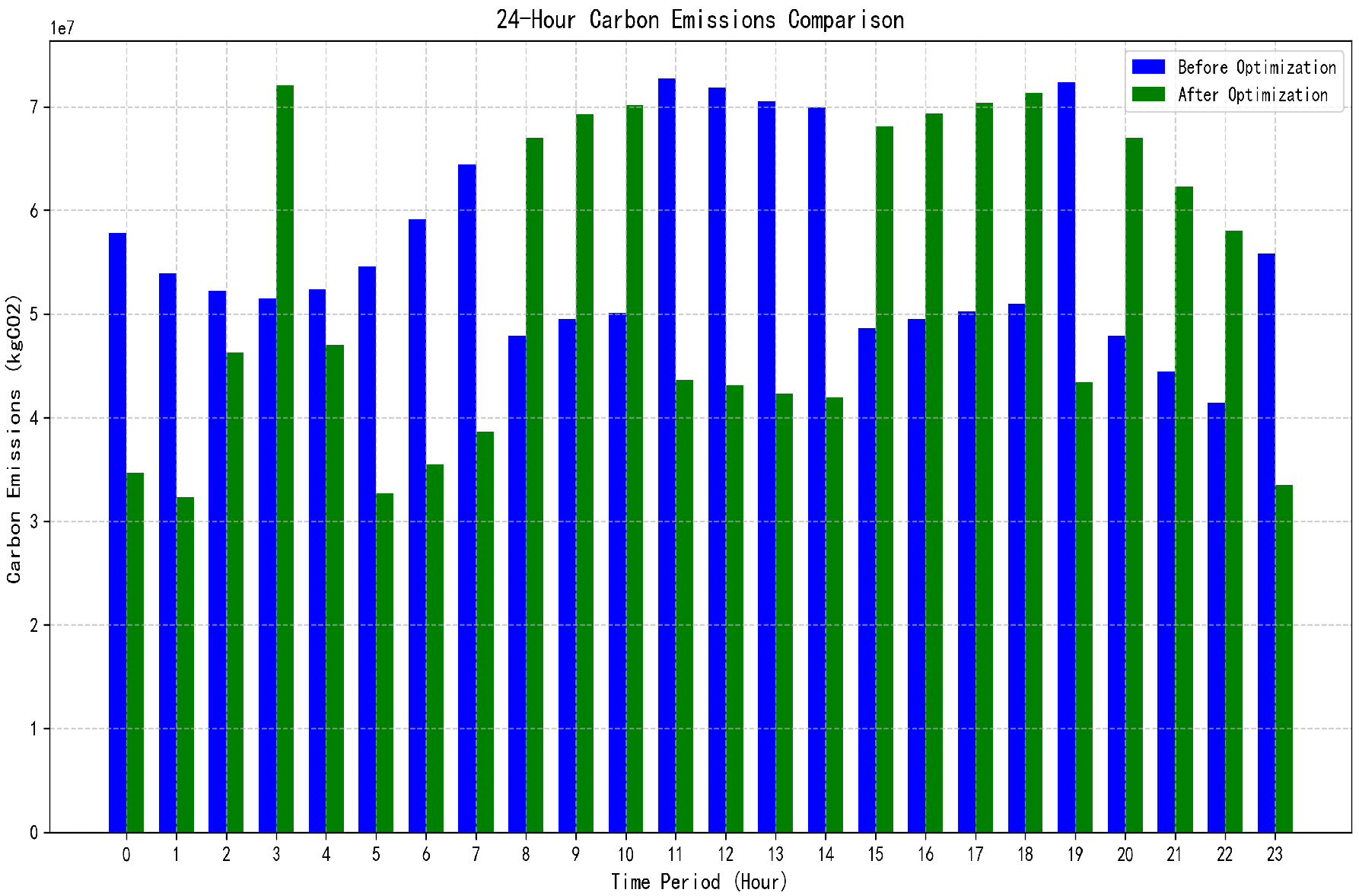
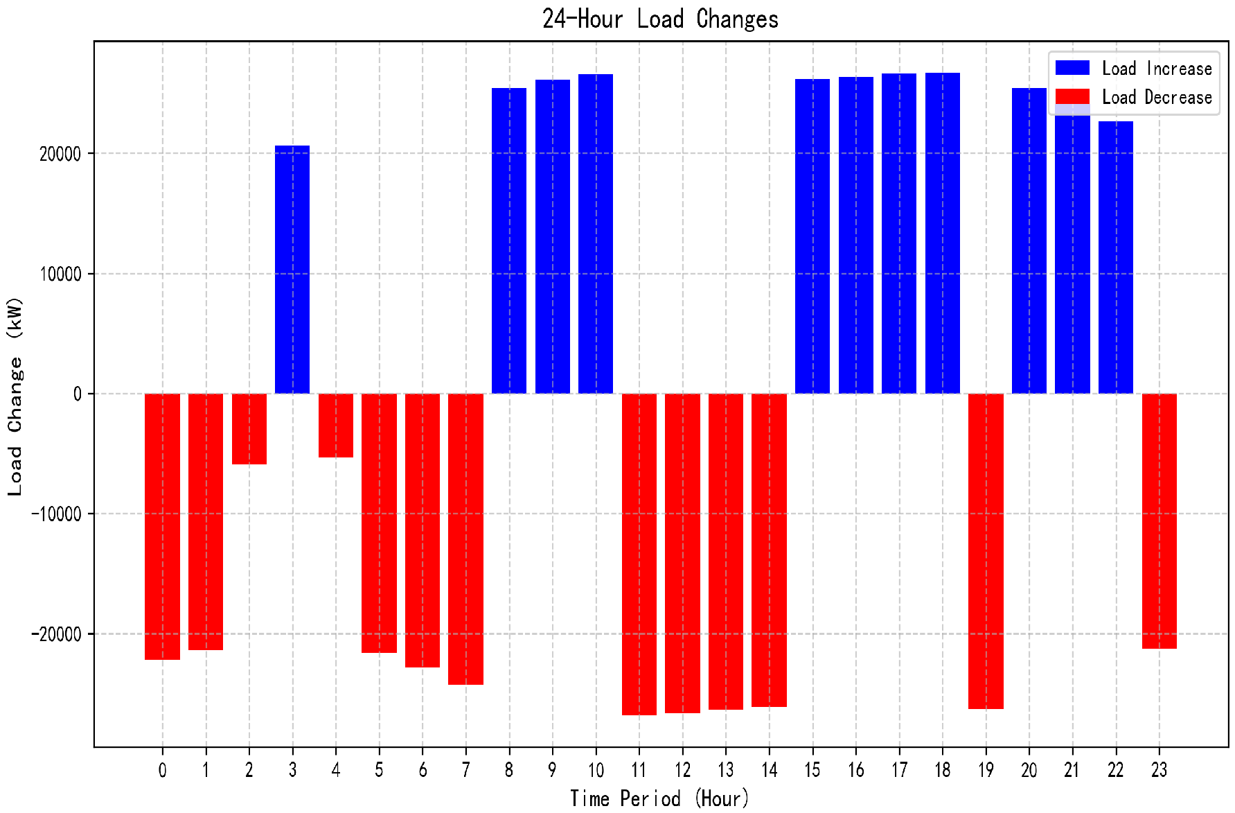
Figure 14 uses a bar chart to compare the changes in total carbon emissions before and after optimization. The carbon emissions before optimization were about $1.33$ units, which were reduced to about $1.26$ units after optimization, achieving an overall emission reduction effect of about $5.95\%$. Figure 15 shows the optimization effect of carbon emissions in each hour. It can be seen from Figure 15 that the emission reduction effect brought by optimization is most significant during peak power consumption hours, such as noon and evening. Figure 16 is a 24-h carbon emission change analysis chart. It can be observed from Figure 16 that the change in carbon emissions is relatively small during the late night and early morning hours, while the optimization effect is very significant during working hours and evening peak hours. This detailed time period analysis helps us adjust the power consumption strategy more accurately and achieve more effective energy conservation and emission reduction.

Table 4. Summary of Demand Response Optimization Results.

Indicator	Before Optimization	After Optimization
Total Carbon Emissions	133,884,203.90	126,218,452.24
Indicator	Change	Change (%)
Total Carbon Emissions	−7,665,751.66	−5.95%

summarizes the effectiveness of the proposed low-carbon demand response optimization strategy by detailing the impact on total carbon emissions. The table contrasts the system’s emissions before and after applying the optimization, presenting the initial value, the optimized value, the absolute reduction achieved, and the corresponding percentage decrease for the primary indicator, total carbon emissions. The optimization resulted in a substantial reduction of approximately $7.67$ million kgCO₂, corresponding to a $5.95\%$ decrease compared to the baseline scenario.

5.4. Discussion

The framework proposed in this paper demonstrates significant advantages over existing methods in both carbon emission assessment and load forecasting. Regarding assessment methods, our DCEF model overcomes the limitations of single methods by dynamically integrating marginal and average carbon emission factors. Unlike the methods of [13], which rely solely on ACEF and fail to capture marginal effects, study [15] relies solely on MCEF susceptible to noise. Our approach provides a more robust and accurate carbon signal. Similarly, in terms of forecasting models, our DPMM-LSTM framework demonstrates superior accuracy. Traditional deep learning models, such as the method proposed in [21], can process time series but struggle to adaptively distinguish data features under different operating modes. Our approach pre-clusters patterns using the DPMM, providing key feature inputs to the LSTM. This results in significantly lower forecasting error (MAE of $185.5$) than the baseline LSTM model (MAE of $240.8$), particularly improving its ability to capture peak-to-valley variations.

The optimization results of this study confirm that by shifting the power load from high-carbon emission periods to low-carbon emission periods, significant emission reduction effects can be achieved. Based on this, we make two suggestions:

(1) Provide users with carbon intensity forecasts: Grid companies or relevant institutions can release grid carbon intensity forecast information for the next 24 h to users. This can help environmentally conscious users or users with smart homes to independently arrange non-emergency electricity tasks such as charging and washing during periods when the grid is cleaner.

(2) Optimize the design of demand response projects: Our results show that the emission reduction potential obtained through load adjustment is the greatest during peak power consumption periods such as evening. Therefore, the incentive mechanism of demand response projects can be more targeted, which focuses on encouraging large adjustable loads such as industry and commerce to participate in reductions during these key high-carbon periods, thereby maximizing the efficiency and effectiveness of emission reduction.

6. Conclusions

This study developed a low-carbon demand response resource optimization dispatch method based on dynamic CEFs. By establishing a dynamic carbon emission factor evaluation model, it effectively integrated both marginal and average carbon emissions. The introduction of the DPMM achieved adaptive clustering of carbon emission patterns and power consumption characteristics, based on which a dual LSTM deep learning network architecture is designed for coordinated prediction of power consumption and carbon emission factors. The study constructed a demand response optimization model aimed at maximizing carbon emission reduction. Case analysis verified the effectiveness of the method in reducing system carbon emissions while ensuring user comfort and equipment safety.

However, this study has limitations that point to future improvements. The simplified DCEF model should be enhanced with additional economic factors. Furthermore, the prediction model could be improved through more sophisticated feature engineering to better capture the underlying context from available data. A key next step is to validate the framework’s robustness and generalizability on more diverse and extensive datasets.

References

1. Wang, N.; Chang, Y. The Evolution of Low-Carbon Development Strategies in China. Energy 2014, 68, 61–70. [Google Scholar] [CrossRef]
2. Ding, C.; Chen, H.; Liu, Y.; Hu, J.; Hu, M.; Chen, D.; Irfan, M. Unleashing Digital Empowerment: Pioneering Low-Carbon Development Through the Broadband China Strategy. Energy 2024, 295, 131034. [Google Scholar] [CrossRef]
3. Ma, F.; Ying, L.; Cui, X.; Lu, W.; Zhang, X.; Wang, H. Research on a Low-Carbon Optimization Strategy for Regional Power Grids Considering a Dual Demand Response of Electricity and Carbon. Sustainability 2024, 16, 7000. [Google Scholar] [CrossRef]
4. Xiao, P.; Xu, J.; Yu, Z.; Qian, P.; Lu, M.; Ma, C. Spatiotemporal Pattern Differentiation and Influencing Factors of Cultivated Land Use Efficiency in Hubei Province Under Carbon Emission Constraints. Sustainability 2022, 14, 7042. [Google Scholar] [CrossRef]
5. Mostafaeipour, A.; Bidokhti, A.; Fakhrzad, M.B.; Sadegheih, A.; Mehrjerdi, Y.Z. A New Model for the Use of Renewable Electricity to Reduce Carbon Dioxide Emissions. Energy 2022, 238, 121602. [Google Scholar] [CrossRef]
6. Kenari, M.B.; Barforoushi, T. Optimal Scheduling of Demand Response Contracts for a Strategic Aggregator in Wholesale Electricity Market. Int. J. Electr. Power Energy Syst. 2025, 169, 110784. [Google Scholar] [CrossRef]
7. Li, X.; Zhang, F.; Huang, Y.; Zhang, G. Bi-Level Sustainability Planning for Integrated Energy Systems Considering Hydrogen Utilization and the Bilateral Response of Supply and Demand. Sustainability 2025, 17, 7637. [Google Scholar] [CrossRef]
8. Blouch, N.; Kazmi, S.N.H.; Metwaly, M.; Akram, N.; Mi, J.; Hanif, M.F. Towards Sustainable Construction: Experimental and Machine Learning-Based Analysis of Wastewater-Integrated Concrete Pavers. Sustainability 2025, 17, 6811. [Google Scholar] [CrossRef]
9. Althaher, S.; Mancarella, P.; Mutale, J. Automated Demand Response from Home Energy Management System Under Dynamic Pricing and Power and Comfort Constraints. IEEE Trans. Smart Grid 2015, 6, 1874–1883. [Google Scholar] [CrossRef]
10. Zhang, M.; Yang, Y.; Xia-Bauer, C. Measuring urban low-carbon sustainability in four Chinese cities. Sustainability 2021, 13, 12281. [Google Scholar] [CrossRef]
11. Meng, C.; Du, X.; Zhu, M.; Ren, Y.; Fang, K. The Static and Dynamic Carbon Emission Efficiency of Transport Industry in China. Energy 2023, 274, 127297. [Google Scholar] [CrossRef]
12. Chen, B.; Ji, X.; Ji, X. Dynamic and Static Analysis of Carbon Emission Efficiency in China’s Transportation Sector. Sustainability 2023, 15, 1508. [Google Scholar] [CrossRef]
13. Dixit, M.K.; Culp, C.H.; Fernandez, J.L. Calculating Primary Energy and Carbon Emission Factors for the United States’ Energy Sectors. RSC Adv. 2014, 4, 54200–54216. [Google Scholar] [CrossRef]
14. Liu, J.; Zhao, H.; Wang, S.; Liu, G.; Zhao, J.; Dong, Z.Y. Real-Time Emission and Cost Estimation Based on Unit-Level Dynamic Carbon Emission Factor. Energy Convers. Econ. 2023, 4, 47–60. [Google Scholar] [CrossRef]
15. Li, J.; Wang, G.; Wang, X.; Du, Y. Smart Charging Strategy for Electric Vehicles Based on Marginal Carbon Emission Factors and Time-of-Use Price. Sustain. Cities Soc. 2023, 96, 104708. [Google Scholar] [CrossRef]
16. Huber, J.; Lohmann, K.; Schmidt, M.; Weinhardt, C. Carbon Efficient Smart Charging Using Forecasts of Marginal Emission Factors. J. Clean. Prod. 2021, 284, 124766. [Google Scholar] [CrossRef]
17. Abonamah, A.; Hassan, S.; Cale, T. Artificial Intelligence and Environmental Sustainability Playbook for Energy Sector Leaders. Sustainability 2025, 17, 6529. [Google Scholar] [CrossRef]
18. Zvierieva, A.; Borziak, O.; Dudin, O.; Panchenko, S.; Rucińska, T. Research on Polyurethane-Stabilized Soils and Development of Quantitative Indicators for Integration into BIM-Based Project Planning. Sustainability 2025, 17, 7781. [Google Scholar] [CrossRef]
19. Duan, J.; Wang, P.; Ma, W.; Tian, X.; Fang, S.; Cheng, Y.; Chang, Y.; Liu, H. Short-Term Wind Power Forecasting Using the Hybrid Model of Improved Variational Mode Decomposition and Correntropy Long Short-Term Memory Neural Network. Energy 2021, 214, 118980. [Google Scholar] [CrossRef]
20. Chi, D.J.; Chu, C.C. Artificial Intelligence in Corporate Sustainability: Using LSTM and GRU for Going Concern Prediction. Sustainability 2021, 13, 11631. [Google Scholar] [CrossRef]
21. Tsokov, S.; Lazarova, M.; Aleksieva-Petrova, A. A Hybrid Spatiotemporal Deep Model Based on CNN and LSTM for Air Pollution Prediction. Sustainability 2022, 14, 5104. [Google Scholar] [CrossRef]
22. Zhang, C.; Li, R. A Novel Closed-Loop Clustering Algorithm for Hierarchical Load Forecasting. IEEE Trans. Smart Grid 2021, 12, 432–441. [Google Scholar] [CrossRef]
23. Gharavi, H.; Hu, B. Space-Time Approach for Disturbance Detection and Classification. IEEE Trans. Smart Grid 2018, 9, 5132–5140. [Google Scholar] [CrossRef]
24. Barrio, I.; Yeo, J.; Janes, J.; Mirdita, M.; Gilchrist, C.L.; Wein, T.; Varadi, M.; Velankar, S.; Beltrao, P.; Steinegger, M. Clustering Predicted Structures at the Scale of the Known Protein Universe. Nature 2023, 622, 637–645. [Google Scholar] [CrossRef]
25. El Araby, E.E.; Yorino, N. A Demand Side Response Scheme for Enhancing Power System Security in the Presence of Wind Power. Int. J. Electr. Power Energy Syst. 2023, 146, 108714. [Google Scholar] [CrossRef]
26. Kini, R.L.; Vlachokostas, A.; Brambley, M.R.; Rogers, A. Occupant-Centric Demand Response for Thermostatically-Controlled Home Loads. IEEE Trans. Smart Grid 2025, 16, 2234–2245. [Google Scholar] [CrossRef]
27. Kwon, S.; Ntaimo, L.; Gautam, N. Demand Response in Data Centers: Integration of Server Provisioning and Power Procurement. IEEE Trans. Smart Grid 2019, 10, 4928–4938. [Google Scholar] [CrossRef]
28. Mobarakeh, A.I.; Sadeghi, R.; Delshad, M. Techno-Economic Energy Management of Micro-Grid in the Presence of Distributed Generation Sources Based on Demand Response Programs. Int. J. Electr. Power Energy Syst. 2022, 141, 108169. [Google Scholar] [CrossRef]
29. Yang, P.; Jiang, H.; Liu, C.; Kang, L.; Wang, C. Coordinated Optimization Scheduling Operation of Integrated Energy System Considering Demand Response and Carbon Trading Mechanism. Int. J. Electr. Power Energy Syst. 2023, 147, 108902. [Google Scholar] [CrossRef]
30. Guo, Z.; Zhang, R.; Wang, L.; Zeng, S.; Li, Y. Optimal Operation of Regional Integrated Energy System Considering Demand Response. Appl. Therm. Eng. 2021, 191, 116860. [Google Scholar] [CrossRef]
31. Yang, M.; Liu, Y. Research on Multi-Energy Collaborative Operation Optimization of Integrated Energy System Considering Carbon Trading and Demand Response. Energy 2023, 283, 129117. [Google Scholar] [CrossRef]
32. Chang, H.; Ding, Q.; Zhao, W.; Hou, N.; Liu, W. The Digital Economy, Industrial Structure Upgrading, and Carbon Emission Intensity: Empirical Evidence from China’s Provinces. Energy Strategy Rev. 2023, 50, 101218. [Google Scholar] [CrossRef]
33. Li, Y.; Yang, X.; Ran, Q.; Wu, H.; Irfan, M.; Ahmad, M. Energy Structure, Digital Economy, and Carbon Emissions: Evidence from China. Environ. Sci. Pollut. Res. 2021, 28, 64606–64629. [Google Scholar] [CrossRef] [PubMed]
34. Neal, R.M. Markov Chain Sampling Methods for Dirichlet Process Mixture Models. J. Comput. Graph. Stat. 2000, 9, 249–265. [Google Scholar] [CrossRef]
35. Boggs, P.T.; Tolle, J.W. Sequential Quadratic Programming. Acta Numer. 1995, 4, 1–51. [Google Scholar] [CrossRef]
Figure 1. The framework diagram of this paper.
Sustainability 17 09123 g001
Figure 2. Power consumption clustering results.
Sustainability 17 09123 g002
Figure 3. DCEF clustering results.
Sustainability 17 09123 g003
Figure 4. Changes in power consumption of the cluster center.
Sustainability 17 09123 g004
Figure 5. Changes in DCEFs of the cluster center.
Sustainability 17 09123 g005
Figure 6. Loss curve diagram of power consumption prediction.
Sustainability 17 09123 g006
Figure 7. Loss curve diagram of CEFs prediction.
Sustainability 17 09123 g007
Figure 8. Comparison results of DCEF prediction.
Sustainability 17 09123 g008
Figure 9. Comparison results of power consumption prediction.
Sustainability 17 09123 g009
Figure 10. Loss curve diagram of power consumption prediction of Italy.
Sustainability 17 09123 g010
Figure 11. Loss curve diagram of CEF prediction of Italy.
Sustainability 17 09123 g011
Figure 12. Comparison results of DCEF prediction of Italy.
Sustainability 17 09123 g012
Figure 13. Comparison results of power consumption prediction of Italy.
Sustainability 17 09123 g013
Figure 14. Comparison of total carbon emissions before and after optimization.
Sustainability 17 09123 g014
Figure 15. Comparison of hourly carbon emissions before and after optimization.
Sustainability 17 09123 g015
Figure 16. Hourly carbon emissions change chart before and after optimization.
Sustainability 17 09123 g016