Abstract
As the global climate continues to warm, continuous high-temperature heat waves have a significant impact on urban socio-economic and sustainable development. Based on the relationship equation between the WBGT index and labor productivity, this paper estimates the economic losses caused by high temperature in 278 cities in China, and investigates the spatial-temporal evolution of the urban economic losses. The main conclusions are as follows: (1) Nationally, the secondary industry experiences the highest average economic losses. Cities in southern, eastern, and central China exhibit the greatest vulnerability, necessitating prioritized climate adaptation planning. (2) Temporally, the average economic losses due to high temperature in Chinese cities from 2010 to 2020 showed a fluctuating upward trend, increasing from 1.343 billion yuan in 2010 to 5.557 billion yuan in 2020. The national average WBGT index increased by 1.69 °C between 2010 and 2020. For every 1 °C increase in the WBGT index, the national economic loss is projected to increase by 0.249 billion yuan. (3) Spatially, areas with high average economic losses were predominantly concentrated in eastern regions, whereas western and central regions exhibited relatively lower losses. The northeastern region recorded the lowest average economic losses. (4) The center of economic loss shifted southwestward from Huangshi City (2010) to Jiujiang City (2020), with an overall migration distance of 143.37 km. The migration velocity exhibited a decelerating trend. This study aims to provide insights for formulating differentiated regional climate adaptation policies and advancing the development of sustainable cities that are resilient to high temperatures while balancing social equity and economic stability.
1. Introduction
With the continuous warming of the global climate and the frequent occurrence of extreme high temperatures, the economic development of human societies is seriously threatened. The Intergovernmental Panel on Climate Change (IPCC) pointed out in its Sixth Assessment Report Synthesis [1] that extreme weather is exerting increasingly dangerous impacts on nature and people in every region of the world, and that the current global average temperature is 1.1 °C higher than pre-industrial levels. The potential global income loss from reduced labor capacity during extreme heat events is estimated at 863 billion dollars, with the most severe impacts in the agricultural sector [2]. The Lancet Countdown to China Report, published in 2023, showed that the potential loss of labor time due to heat exposure for the year 2022 is 38.3 billion hours, averaging 46.6 h per worker, with associated economic loss amounting to approximately 3055 dollars. Labor productivity is defined as the ratio of the output created by a worker in a given period of time to the total amount of labor he or she consumes. At the macroeconomic level, it is typically measured by output per hour worked or production per employer [3]. Yaglou and Minard introduced the Wet Bulb Globe Temperature (WBGT) index in 1957 [4], which was accepted by the International Organization for Standardization (ISO) and the U.S. Conference of Governmental Industrial Hygienists as a tool for assessing hot environments [5]. High temperatures affect the urban economy through both direct and indirect pathways [6,7,8,9,10]. High-temperature heat waves can affect the physiological health of workers, including chronic diseases, heat-related illnesses (e.g., heat exhaustion, pyrexia), and cardiovascular, cerebrovascular, and respiratory conditions [11,12,13,14,15,16]. At the same time, long-term high-temperature environments can also negatively affect the mental health of workers [17,18], such as emotional fluctuations, irritability, depression, etc., and these psychological problems can also affect labor productivity (Figure 1).
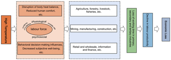
Figure 1.
Framework for analyzing the indirect impact of high temperature on the regional economy.
Related studies have shown that outdoor work sectors such as agriculture, manufacturing, and services are particularly affected by heat-related productivity losses, and that these sectors rely on physical labor, which is more risky in high-temperature environments [19]. In addition, the economic impact of heat-related labor productivity losses varies in different regions due to differences in climatic conditions and levels of economic development [20,21,22,23,24,25,26]. Zander et al. [27] found that the annual economic burden caused by hot weather in Australia during 2013–2014 was approximately 6.2 billion dollars. Recent studies in China have expanded this research scope. Chen et al. [28] demonstrated that from 2013 to 2019, Wuhan experienced an average of 77,369 heat-related premature deaths annually, with associated economic losses reaching 156.1 billion yuan. In summary, existing research has laid an important foundation for understanding the economic impacts of high temperatures. However, these analyses are largely built upon the implicit assumption that the effects of climate shocks are relatively homogeneous, and they generally emphasize the dominant vulnerability of the agricultural sector. The aforementioned theoretical framework faces challenges when applied to explain China, a massive economy characterized by significant regional development imbalances.
In view of this, this study aims to systematically address the following three core questions: (1) What are the characteristics of the spatiotemporal evolution patterns of economic losses from high temperatures in Chinese cities between 2010 and 2020? Is their spatial distribution random, or does it exhibit significant clustering? (2) How do different industrial sectors contribute to total economic losses? Is agriculture the dominant contributor, as traditionally perceived? (3) How has the spatial center of economic losses from high temperatures shifted over the decade? What regional risk trends does this migration reveal?
Considering that the economy and labor productivity are significantly impacted by high temperatures, this study used the WBGT index to estimate economic loss data from heatwaves across 278 Chinese cities during the 2010–2020 period. By employing spatial autocorrelation analysis, spatio-temporal transition matrix, and Standard Deviation Ellipse (SDE) model, we examine the spatiotemporal dynamics and centroid migration patterns of economic losses over the past decade. The findings provide clear practical guidance for formulating differentiated regional climate adaptation policies and safeguarding the rights of outdoor workers, thereby advancing the development of sustainable cities resilient to high temperatures while balancing social equity and economic stability.
2. Materials and Methods
2.1. Study Area
This study takes cities as the research unit and selects the administrative scope of cities in 2019 for data organization. Given differences in statistical systems, data dissemination channels, and meteorological observation networks between Hong Kong, Macau, and Taiwan regions and mainland China, we have not included these areas in the current analysis to maintain consistency in model calculations and result comparisons. Excluding areas with missing data, a total of 278 Chinese cities were selected as research objects for the study (Figure 2), with a time span of 2010, 2015, and 2020.
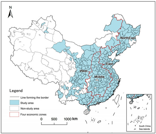
Figure 2.
Study area.
2.2. Data Sources
The administrative boundary data were obtained from the Standard Map Service System of the Ministry of Natural Resources (http://bzdt.ch.mnr.gov.cn/). The temperature data were obtained from the meteorological dataset issued by the National Center for Environmental Information (NCEI) under the National Oceanic and Atmospheric Administration (NOAA) of the United States (https://www.ncei.noaa.gov/), and the humidity data were sourced from the daily value dataset of Chinese ground climate data (V3.0) issued by the China Meteorological Data Sharing Network (http://data.cma.cn). By filtering and organizing data, we obtained daily relative humidity and maximum temperature data for each city from 2010 to 2020. The employment situation of the three industries in each city is sourced from the China Urban Statistical Yearbook. The minimum hourly wage standard in cities is derived from the China Research Data Service Platform (https://www.cnrds.com).
2.3. Research Methods
2.3.1. Relationship Between WBGT Index and Labor Productivity
The WBGT index, measured in °C, is a heat stress index that combines temperature, humidity, and other environmental factors. The simplified WBGT is a linear combination of air temperature and wet bulb temperature [29]. Labor productivity is affected by working conditions, with a higher WBGT index indicating more frequent pauses, interruptions, lower speeds, and a higher probability of injury. Even though adaptation to the environment and protective measures such as air conditioning can help to suppress the negative effects of heat stress, the effectiveness and applicability of any acclimatization mean is limited and environment-dependent. In China’s “Occupational Exposure Limits for Hazardous Factors in the Workplace Part 2: Physical Factors” (GBZ2.2-2007) [30], jobs with an average WBGT index greater than 25 °C in the workplace are defined as high-temperature jobs. The ratio of the time that a worker spends in high-temperature operations in a workday to 8 h is defined as labor productivity, and different limits for the WBGT index in different workplaces are specified (Table 1). Under the same physical labor intensity, the higher the WBGT index, the lower the labor productivity, and similarly, under the same labor productivity conditions, the higher the physical intensity, the lower the WBGT index limit.

Table 1.
Limits of WBGT index for different physical labor intensities (°C).
For this reason, Kjellstrom et al. assumed that 200 W corresponds to the service industry, 300 W corresponds to manufacturing jobs, 400 W corresponds to agricultural jobs, etc., and categorized the different labor intensities according to the corresponding industries [31]. Based on Kjellstrom’s study, Roson et al. [32] used the overall average to determine the functional relationship between the WBGT index and labor productivity in the three industries (Figure 3), and proposed that the minimum value of the WBGT index for agriculture, manufacturing and service industries are 26 °C, 28 °C and 30 °C, respectively. When the minimum labor productivity is 25%, the corresponding WBGT indices for agriculture, manufacturing and service industries are 36 °C, 43 °C and 50 °C, respectively.
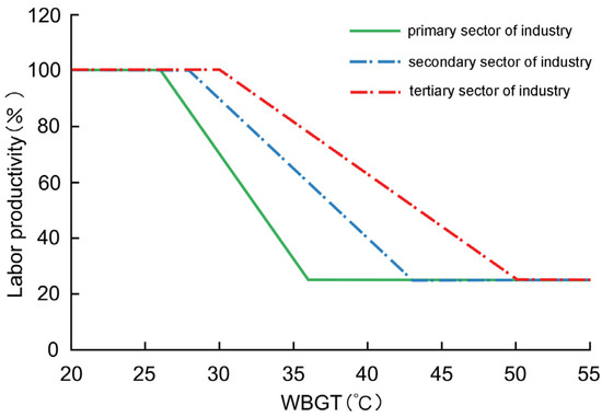
Figure 3.
Variation in labor productivity with WBGT (according to Roson et al. [32]).
2.3.2. Methodology for Assessing Economic Losses Under the Influence of High Temperature
- (1)
- WBGT index
Due to the difficulty in obtaining black globe temperature, direct measurements of the WBGT index are rare. Therefore, this paper employs a method proposed by the Australian Bureau of Meteorology to estimate WBGT based on meteorological data. This WBGT calculation method has been validated as an alternative for assessing heat stress in outdoor workplaces [33,34,35]. The WBGT index depends solely on temperature and humidity, representing thermal stress under average daytime outdoor conditions:
In the equation, represents the near-surface air temperature (°C), denotes the vapor pressure, which is calculated using Formula (2), is the relative humidity (%):
- (2)
- Labor productivity loss
On the basis of calculating the WBGT index, the labor productivity loss is calculated with reference to the relationship equation between the WBGT index and labor productivity of the three industries established by Roson et al. [32]:
where is the value of labor productivity loss; , , denote the first, second and third industry, respectively.
On the basis of calculating the daily labor productivity loss, combined with the number of days affected by high temperature, the annual labor productivity loss of each industry can be obtained:
where , , represents the total annual labor productivity losses of the first, second and third industry, respectively, in the city under the influence of high temperature; n is the number of days; lab is the daily loss of labor productivity in different industries.
Based on the number of people employed in the city’s three industries, the overall lost labor productivity of the city can be obtained:
where is the total amount of labor productivity lost in the city; , , , are the number of people employed in the three industries; , , , are the loss of labor productivity in the three industries, respectively.
- (3)
- Estimation of regional economic loss value
Referring to the 8 h legal working hours a day stipulated by the Chinese labor law in Table 1, the formula for the total economic loss value of the region is.
where EL stands for the value of regional economic losses; is the total labor productivity loss in city ; and is the minimum hourly wage standard in city .
When estimating economic losses, we multiply the lost labor hours by each city’s hourly minimum wage rate. This approach is primarily based on the following considerations: (1) Using the minimum wage for estimation avoids overestimating losses, yielding more robust and conservative results; (2) Minimum wage rates across cities are officially published, standardized data that are easily accessible and comparable, making them suitable for large-scale cross-city research; (3) Extreme heat disproportionately impacts outdoor workers, whose compensation levels often align closely with minimum wage standards. Thus, this metric better reflects the economic impact on vulnerable groups.
2.3.3. Research Method for the Spatial and Temporal Dynamic Evolution of Economic Losses
- (1)
- Spatial autocorrelation analysis
Considering the temporal evolution and dynamic transition characteristics of economic losses caused by urban high temperatures, global and local spatial autocorrelation tests are used to examine the similar and dissimilar characteristics between neighboring areas in the entire region or local area. Perform significance testing by calculating Z-scores and p-values.
where represents the number of cities (278), while and represent the economic loss values for cities and respectively, and denote the mean and variance of economic losses across all cities, and constitutes the spatial weight matrix.
Given that heatwaves are regional climate phenomena, economic linkages such as labor markets and industrial chains typically diminish with distance. Therefore, this paper employs a distance-based weight matrix as its core analytical framework to evaluate each factor within the adjacent element environment. Neighboring factors within a specified critical distance will be assigned a weight of 1, influencing the calculation of the target factor. Neighboring factors beyond the specified critical distance will be assigned a weight of 0 and will have no impact on the calculation of the target factor.
where is the distance between the centroids of city and city .
- (2)
- Standard deviation ellipse and center of gravity modeling
The SDE can measure the dynamic evolution trend of economic losses, and this paper utilizes ArcGIS 10.8 to calculate indicators such as the long axis, short axis, and azimuthal angle of the ellipse and their changes. The major axis and minor axis of the SDE represent the dispersion of geographic features along primary and secondary directions, respectively. The centroid indicates the relative spatial position of geographic features, while the azimuth reflects the predominant directional trend of their distribution.
- (3)
- Local Indicators of Spatial Association (LISA) Spatial-temporal transition
LISA spatio-temporal transition reflects the spatio-temporal evolution characteristics of Local Moran’s I scatter plot, which can be divided into four types [36]: Type I refers to the transition of the city itself, with no transition in the neighboring cities; Type II refers to the stability of the city itself, and the transition of the neighboring cities; Type III refers to the transition between a city and its neighboring cities; Type IV refers to cities that have not transitioned from neighboring cities (Table 2).
Table 2.
Type of LISA spatio-temporal transition.
The spatial and temporal cohesion index is used to calculate the stability of the spatial distribution of urban economic losses under the influence of high temperature, and the formula is:
where and are the transition numbers of types I and IV, respectively, in the study period; m is the total number of cities in the study unit.
3. Results and Analysis
3.1. Spatial and Temporal Evolution of Economic Losses
3.1.1. Characteristics of Temporal Evolution of Economic Loss
Overall, the economic losses of Chinese cities have been fluctuating and continuously increasing from 2010 to 2020 (Table 3 and Figure 4a). Among them, the economic losses from 2013 to 2015 and from 2018 to 2019 were in a declining stage. The average value of urban economic loss rose from 1.343 billion yuan to 2.589 billion yuan from 2010 to 2013, with an average annual increase of 30.93%. From 2013 to 2019, the overall change in urban economic losses remained stable, with an average of 4.34 billion yuan. From 2019 to 2020, the average value of the city’s economic losses increased from 4.25 billion yuan to 5.56 billion yuan, an increase of 30.82%. According to the geographic division of China’s economic regions, the average economic losses of cities in the eastern region are significantly higher than those in other regions, and the fluctuation value is larger. This is mainly due to the existence of multiple mega cities in the eastern region, which have a higher level of socio-economic development, and the industrial structure is mostly based on the secondary and tertiary industries.
Table 3.
Average economic losses in China and the four major regions are under the impact of high temperatures.
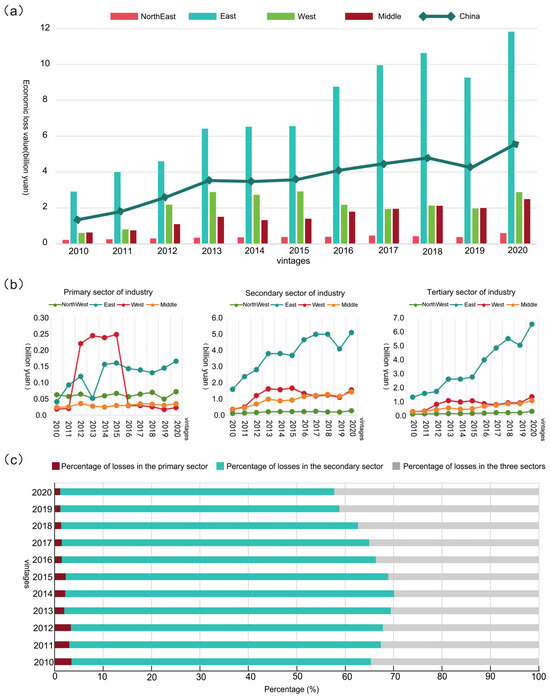
Figure 4.
Characteristics of time-series changes in high-temperature economic losses. (a) Average economic losses in China and the four major regions under the impact of high temperatures, 2010–2020. (b) Average economic losses in the three industries in the four regions, 2010–2020. (c) Percentage of average value of economic losses in China’s three industries, 2010–2020.
The total economic loss of the secondary industry in the four major regions is greater than that of either the tertiary industry or the primary industry (Figure 4b), possibly due to the higher intensity of labor required by this industry and more outdoor work activities. The average value of economic losses in the secondary and tertiary industries in the eastern region far exceeds that of the other three regions, especially after 2015. In stages, the average value of economic losses in the primary industry in the western region is larger than that in the other three regions in 2012–2015, exceeding 0.2 billion yuan. The average value of economic loss in the three industries in the western and central regions remained basically the same from 2016 to 2020, while the average value of economic losses in the secondary and tertiary industries in the eastern region shows an N-shaped fluctuation.
From a national perspective, the average economic losses of the secondary industry are the highest, followed by the average economic losses of the secondary industry, and the average economic losses of the primary industry are the lowest (Figure 4c). The characteristics of the average economic losses of the three industries in the four major regions are the same, with the average economic losses of the secondary industry accounting for more than 50% for ten consecutive years.
3.1.2. Characteristics of the Spatial Evolution of Economic Losses
During the study period, the average value of the national WBGT index increased year by year. Compared to 2010, the average value of the national WBGT index in 2020 increased by 1.69 °C (Figure 5a). Using formulas to calculate, the economic losses of 278 cities above prefecture level in China under the influence of high temperature from 2010 to 2020 is derived (Figure 5b), and the proportion of economic losses to urban GDP is also calculated to reflect the degree of influence of high temperature on the economy of each city. In 2010, there were two cities whose economic losses were in the high value zone, namely Guangzhou and Shenzhen, with total economic losses amounting to 10.13 billion yuan and 9.75 billion yuan, respectively. In 2015, a total of 11 cities were in the high economic loss zone, including Shenzhen, Guangzhou, Chongqing, Shanghai, Dongguan, and Foshan, among others. The economic losses of all these cities exceeded 223.65 million yuan, with Shenzhen reaching the highest of 677.88 million yuan. In 2020, a total of 21 cities were in the high economic loss zone, with the top ten cities including Shenzhen, Shanghai, Guangzhou, Chengdu, Beijing, Dongguan, Chongqing, Suzhou, Hangzhou, and Fuzhou. All of these cities suffered economic losses of more than 15 billion yuan, with Shenzhen having the highest loss, reaching 45.44 billion yuan. Overall, the losses caused by high temperatures to China’s urban economy intensified year by year during the research period, with cities along the southeastern coast being the most severely affected, and gradually spreading to inland and northern cities.
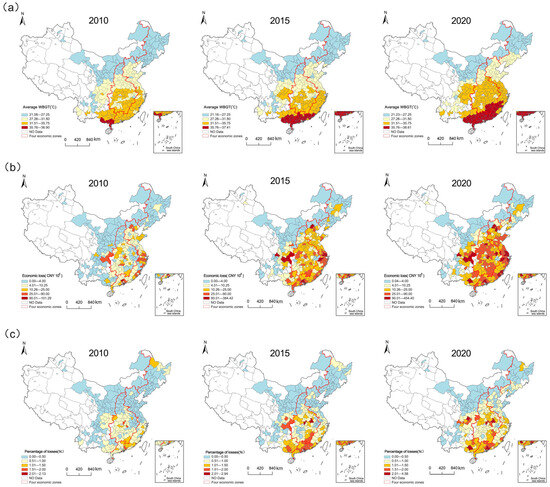
Figure 5.
Characterization of spatial variability in high-temperature economic losses. (a) Average WBGT index for China, 2010–2020. (b) Value of economic losses by city under the impact of high temperatures, 2010–2020. (c) Economic losses as a share of GDP in cities affected by high temperatures, 2010–2020.
From 2010 to 2020, the distribution map of the proportion of urban GDP losses caused by high temperature shows (Figure 5c) that the high loss area is mainly concentrated in the southeast, but there is a significant difference in the spatial distribution and number of cities with economic losses caused by high temperature. In 2010, the proportion of economic losses to GDP in 7 cities was higher than the average value of the cities; in 2015, 8 cities were classified as high proportion areas, including Dongguan, Xiamen, Haikou, Zhuhai, Lu’an, Shenzhen, Shantou, and Xiaogan; there were a total of 23 cities with higher values, mainly scattered in provinces such as Chongqing, Jiangxi, Guangxi, and Guangdong; in 2020, the number of cities within the high value zone decreased to 7, including Lu’an, Bazhong, Dongguan, Haikou, Nanning, Xiaogan and Huizhou; there are 25 cities with relatively higher values, mainly distributed in Hubei, Jiangxi, Fujian, Sichuan, and Guangdong provinces. The comparison shows that many cities in the country suffered a relatively high proportion of economic losses to GDP caused by hot weather during the period between 2015 and 2020, and the cities with high economic losses were concentrated, especially in the southeastern region, where the impact was severe. High temperatures have serious consequences for cities with significant economic impacts (mainly large cities). These cities have developed socio-economic levels, with the tertiary industry being the dominant industry. Although high temperatures have caused significant economic losses to these cities, their GDP scales are relatively large, and they have strong climate adaptation capabilities, so the proportion of economic losses caused by high temperatures is relatively low.
3.1.3. Migration Characteristics of the Center of Gravity of Economic Losses
The center of gravity of urban economic loss under the influence of high temperature from 2010 to 2020 has basically shifted to the southwest. It was located in Huangshi City (115.61, 30.47) in 2010, and shifted to Jiujiang City (114.95, 29.34) in 2020 (Figure 6). It shows that the growth rate of economic loss in the western and southern cities is higher than the average level, and the migration speed of the center of gravity first rises and then falls, with a cumulative migration distance of 143.37 km. Specifically, the center of gravity shifted towards the southwest by 80.39 km from 2010 to 2015, and it shifted towards the southwest by 62.97 km from 2015 to 2020.
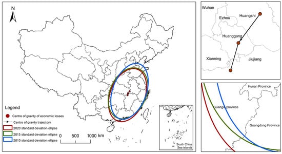
Figure 6.
Standard deviation ellipse and center of gravity shift trajectory of economic loss in Chinese cities under the impact of high temperature, 2010–2020.
The azimuth angle has shown a gradually increasing trend in the last 10 years. It increased from 20.49° in 2010 to 21.52° in 2015 and then to 24.23° in 2020, and the spatial pattern of “northeast–southwest” has not changed significantly. The major axis of the ellipse has shortened from 963.48 km in 2010 to 886.73 km in 2020, and the minor axis has increased from 558.14 km in 2010 to 575.85 km in 2020, indicating that the distribution of the economic losses is becoming more and more concentrated in the north–south direction and more dispersed in the east–west direction (Table 4).
Table 4.
Standard deviation ellipse parameters of economic losses in Chinese cities under the impact of high temperatures, 2010–2020.
3.2. Dynamic Transitions in Economic Losses
3.2.1. Spatial Auto-Correlation Test
Before conducting the analysis of spatio-temporal dynamics, a global spatial auto-correlation test is needed to determine whether the urban economic losses under the influence of high temperature have spatial correlation. Table 5 shows the results of global Moran’s I values for 278 cities. It can be observed that the global Moran’s I of urban economic losses is greater than 0 at all three time points, and the significance level was tested at 0.01, indicating a positive spatial correlation of urban economic losses under the influence of high temperature. There is a trend of high (or low) economic losses in urban agglomeration, which is not randomly distributed. In the time series, the global Moran’s I exhibits a “∽” shaped fluctuation, decreasing from 0.208 in 2010 to 0.131 in 2012, and then rebounding to 0.310 in 2020. This indicates that the spatial correlation between high temperature and the economic loss of Chinese cities is gradually strengthening.
Table 5.
Global Moran’s I and its test results for economic losses by city under the impact of high temperature, 2010–2020.
3.2.2. Dynamic Transition Results
According to the global Moran’s I, the spatial clustering characteristics of economic losses in Chinese cities are significant. Therefore, this study utilizes local Moran’s I maps for 2010, 2015, and 2020 to reveal the transitional characteristics of dynamic loss to the urban economy caused by high temperature. Figure 7 illustrates the LISA map of economic losses caused by high temperatures in Chinese cities, revealing a single spatial clustering pattern of high temperature economic losses with local spatial autocorrelation. The main types are high–high agglomeration (HH) and low–low agglomeration (LL). The number of cities with HH agglomeration gradually decreased from 24 in 2010 to 21 in 2015, and then increased to 25 in 2020, while the number of cities with LL agglomeration increased from 74 in 2010 to 76 in 2015, and then decreased to 73 in 2020. The degree of agglomeration in the HH agglomeration area varied slightly, mainly concentrated in the eastern and southern regions, such as Guangdong, Zhejiang, Jiangsu, and Fujian. In the later period, the cities in the LL agglomeration area are mainly distributed in the three northeastern provinces and Shaanxi, Gansu, and Ningxia in the northwestern region. Meanwhile, the number of LL agglomeration areas in the southwest is gradually decreasing.
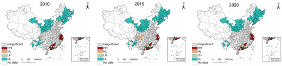
Figure 7.
LISA distribution of economic losses in Chinese cities under the impact of high temperature, 2010–2020.
In this study, the LISA spatio-temporal flow matrix is used to explore the dynamic transition of the spatial agglomeration pattern of urban economic losses caused by high temperature, and the specific details are shown in Table 6. According to Table 6, from 2010 to 2020, the transition pattern of type IV was dominant, with less spatio-temporal transition between different types. The urban economic losses under the influence of high temperature exhibit significant spatial agglomeration and low mobility, and the dynamic transformation pattern had a strong spatial stability. Based on Formula (12), the spatial cohesion index of the three time periods was higher than 93%.
Table 6.
Spatio-temporal transition matrix of economic losses in Chinese cities under the impact of high temperature, 2010–2020.
4. Discussion
4.1. Comparison with Existing Literature
In Southeast Asia, heat-related work time losses have reached 15–20%, and this figure is projected to double by 2050 as climate change persists [37]. Vulnerability to heatwaves is particularly pronounced in low- and middle-income countries. While emission reduction measures and economic development may mitigate impacts to some extent, outdoor labor will remain constrained, and heatwave-related losses will persist significantly [38]. Our research reveals that over the past decade, the center of China’s heat-related economic losses has shifted from Huangshi City to Jiujiang City. This spatio-temporal dynamic perspective offers new insights into the regional imbalance of climate change impacts, addressing the historical neglect of spatial heterogeneity and temporal continuity in conventional studies.
While the existing literature generally emphasizes that the agricultural sector is most affected by high temperatures [2,22], this paper finds that the share of economic losses in the secondary sector (manufacturing and construction) has exceeded 50% for ten consecutive years, especially in the economically developed regions in the east (e.g., Shenzhen and Guangzhou). This finding challenges the traditional perception that “agriculture dominates high-temperature losses”, reveals the complex relationship between industrial structure and climate vulnerability, and provides a new analytical framework for subsequent studies.
Sahu et al. [39] measured hourly heat exposure levels in rice harvesting fields in West Bengal, India. They estimated that productivity declines by approximately 5% for each one-unit increase in the hourly WBGT average. Yi and Chan [40] used a multiple linear regression model to estimate the impact of heat stress on productivity among construction workers in Hong Kong. Results indicated that a 1 °C increase in WBGT reduced productivity by 0.33% due to heat stress. Our findings indicate that for every 1 °C increase in the national WBGT index, the economic losses increase by 0.249 billion yuan. This result provides a reusable parametric tool for the field of climate economics, supporting future studies to incorporate the effects of changing thermal stress dynamics more precisely when predicting economic losses under different warming scenarios.
Through global and local spatial autocorrelation analyses, this paper finds that the high-temperature economic losses in Chinese cities show significant HH and LL clustering patterns, and the spatial and temporal cohesion indices are over 93%, which suggests that the loss distribution is highly stable. This finding verifies the hypothesis of “regional differences in climate adaptive capacity” (e.g., developed cities in the east have lower losses due to stronger economic resilience) and provides empirical support for environmental justice research.
4.2. Implications for Urban Planning and Policy
Policy makers in each city should develop occupational health protection measures according to their own situation, develop regionally differentiated climate adaptation strategies, and prioritize interventions in key areas. South China, East China, and central provinces (e.g., Guangdong, Hubei) need to be prioritized for inclusion in the National Climate Change Action Plan (NCCAP) due to high economic losses and vulnerability. For example, the Pearl River Delta (PRD) region should promote a pilot “heat resilient city” and make it mandatory for new industrial parks to be equipped with shading facilities and distributed cooling systems. Preventive planning for western and northeastern regions: Although losses are currently low, the shift in the center of gravity to the southwest suggests that inland cities need to be alerted to the risk of heat exposure in the future. It is recommended that in emerging growth poles such as the Chengdu-Chongqing Economic Circle, the WBGT index should be incorporated into the evaluation system of territorial spatial planning, to avoid over-concentration of high-labor-intensity industries in high-risk zones of heat stress.
Targeted protection measures for different industries, urban heat stress is more closely associated with industries involving more outdoor work and lower wages than with other industries, and the distribution of economic losses due to future urban warming raises environmental justice issues. Target protection for different industries. The manufacturing and construction sectors need to implement “hot-time flexible working”, for example, by shifting outdoor working hours to early morning or late evening [41,42,43,44,45], and mandating 10–15 min of paid rest per hour. Promote heat-resistant crop varieties through financial subsidies, and encourage service sector companies (e.g., logistics, takeaways) to purchase heat health insurance for their riders to reduce labor risks.
Upgrading the high-temperature warning and health protection system [46], building a nationally unified real-time monitoring platform for high-temperature risk based on the WBGT index, and pushing personalized health advice (e.g., frequency of water replenishment, symptom recognition) to workers via mobile phone APPs. Install additional mobile first aid stations in industrial parks in cities with high heat prevalence (e.g., Guangzhou and Shanghai), and train enterprise safety personnel in initial heat stroke treatment skills.
Improve policies, regulations, and economic incentives by amending the occupational disease prevention and control law to explicitly include pyrexia in the catalog of occupational diseases, and require enterprises to provide cooling equipment for high-temperature jobs and to bear the related medical costs [47,48]. Incorporate the assessment of economic losses from high temperatures into the carbon emissions trading system, and impose a surtax on high-emission enterprises, with the proceeds used to support adaptive infrastructure (e.g., green roofs, permeable pavement) in low-income areas.
4.3. Research Limitations and Future Directions
Although this paper calculates urban economic losses under the influence of high temperatures based on the functional relationship between heat stress and labor productivity, the use of climate model data to calculate WBGT may be biased due to the use of multiple complex algorithms, data and model limitations: the WBGT calculation relies on simplified assumptions of humidity and temperature, which may underestimate the actual heat stress (e.g., not taking into account differences in thermal resistance of clothing). In the future, the model accuracy can be improved by incorporating wearable devices to monitor workers’ microenvironmental data.
The current study focuses on labor productivity loss and does not cover the superimposed effect of high temperature on indirect costs such as energy consumption and medical expenditure. A multi-sectoral Computable General Equilibrium (CGE) model needs to be constructed to comprehensively assess the integrated economic impacts of high temperatures.
Mobile populations (e.g., migrant workers) are vulnerable to high temperature exposure, but their regional migration and loss-sharing mechanisms have not been quantified. A tracking survey is recommended to reveal the feedback relationship between climate risk and labor mobility.
We did not employ Purchasing Power Parity (PPP) for cross-regional adjustments. When comparing total losses across years, this approach may have included price inflation factors. Future studies conducting long-term international comparisons will need to incorporate price indices and PPP into their analyses.
5. Conclusions
This study starts from the perspective of labor productivity, based on the WBGT index, and uses the relationship equation between thermal stress and labor productivity to organize the economic loss data of 278 cities in China under the influence of high temperature from 2010 to 2020. Adopting methods such as spatial autocorrelation, spatio-temporal transition matrix, and standard deviation ellipse model, this study explores the spatio-temporal dynamic evolution of economic loss and center of gravity migration characteristics in Chinese cities under the influence of high temperature in the recent 10 years. The main conclusions are as follows:
- (1)
- In 2010, 2015, and 2020, Guangzhou and Shenzhen ranked among the top three high-value areas for economic losses caused by high temperatures in cities. In 2010, Guangzhou’s highest value was 10.129 billion yuan; in 2015 and 2020, Shenzhen’s highest value reached 38.442 billion yuan and 45.440 billion yuan.
- (2)
- The average WBGT index increased by 1.69 °C from 2010 to 2020, and the average value of economic losses caused by high temperature in Chinese cities from 2010 to 2020 continued to fluctuate. Southeast coastal cities were the most affected, and it was gradually extended to the inland and some of the northern cities. Cities with a high proportion of GDP loss due to high urban temperature are relatively backward in their development levels.
- (3)
- The center of economic losses in Chinese cities has shifted from Huangshi City (2010) to Jiujiang City (2020), and overall, it has moved southwest, the speed of center migration gradually decreases.
- (4)
- The positive spatial correlation of economic damage in Chinese cities is obvious, and the degree of loss is related to the agglomeration distribution of cities, rather than random distribution. Cities with high economic damage showed HH agglomeration and LL agglomeration. Significant regional disparities were observed between northern and southern China, with Type IV transitions as the main type, and almost no spatio-temporal transitions between different types. This suggests that under the influence of temperature, the local spatial correlation patterns of economic losses in Chinese cities show high stability, with specific path correlation or spatial fixation characteristics.
Author Contributions
Conceptualization, X.Y., H.Q. and K.G.; methodology, H.Q.; software, R.Y.; validation, X.Y., K.G. and R.Y.; formal analysis, X.Y.; investigation, H.Q.; resources, X.Y.; data curation, R.Y.; writing—original draft preparation, X.Y. and H.Q.; writing—review and editing, K.G.; visualization, R.Y.; supervision, R.Y.; project administration, K.G.; funding acquisition, K.G. All authors have read and agreed to the published version of the manuscript.
Funding
This research was funded by Ministry of Education of the People’s Republic of China Humanities and Social Sciences Research Project: 24YJA630025.
Institutional Review Board Statement
Not applicable.
Informed Consent Statement
Not applicable.
Data Availability Statement
The original contributions presented in this study are included in the article. Further inquiries can be directed to the corresponding author.
Conflicts of Interest
The authors declare no conflict of interest.
Abbreviations
The following abbreviations are used in this manuscript:
| WBGT | Wet-Bulb Globe Temperature |
| IPCC | Intergovernmental Panel on Climate Change |
| ISO | International Organization for Standardization |
| SDE | Standard Deviation Ellipse |
| NCEI | National Center for Environmental Information |
| NOAA | National Oceanic and Atmospheric Administration |
| LISA | Local Indicators of Spatial Association |
| HH | High–High |
| LL | Low–Low |
| LH | Low–High |
| HL | High–Low |
| CGE | Computable General Equilibrium |
| NCCAP | National Climate Change Action Plan |
| PRD | Pearl River Delta |
| PPP | Purchasing Power Parity |
References
- Lee, H.; Calvin, K.; Dasgupta, D.; Krinner, G.; Mukherji, A.; Thorne, P.; Trisos, C.; Romero, J.; Aldunce, P.; Barret, K. IPCC, 2023: Summary for Policymakers. In Climate Change 2023: Synthesis Report, Contribution of Working Groups I, II and III to the Sixth Assessment Report of the Intergovernmental Panel on Climate Change; Core Writing Team, Lee, H., Romero, J., Eds.; IPCC: Geneva, Switzerland, 2023. [Google Scholar]
- Borg, M.A.; Xiang, J.; Anikeeva, O.; Pisaniello, D.; Hansen, A.; Zander, K.; Dear, K.; Sim, M.R.; Bi, P. Occupational heat stress and economic burden: A review of global evidence. Environ. Res. 2021, 195, 110781. [Google Scholar] [CrossRef]
- Goel, V.; Agrawal, R.; Sharma, V. Factors affecting labour productivity: An integrative synthesis and productivity modelling. Glob. Bus. Econ. Rev. 2017, 19, 299–322. [Google Scholar] [CrossRef]
- Yaglou, C.; Minaed, D. Control of heat casualties at military training centers. AMA Arch. Ind. Health 1957, 16, 302–316. [Google Scholar] [PubMed]
- d’Ambrosio Alfano, F.R.; Malchaire, J.; Palella, B.I.; Riccio, G. WBGT index revisited after 60 years of use. Ann. Occup. Hyg. 2014, 58, 955–970. [Google Scholar] [CrossRef] [PubMed]
- Li, Y.; Liu, C.; Song, Y. Research progress of the impact of frequent high temperature heat waves on economic system. Adv. Clim. Change Res. 2021, 17, 121–130. [Google Scholar]
- Chu, B.-W.; Luo, J.-F.; Wang, K.-X.; Xing, Z.-C.; Wang, H.-K. Substantial increase of heat-induced labor and economic loss in China under rapid economic and environmental temperature growth. Adv. Clim. Change Res. 2024, 15, 708–716. [Google Scholar] [CrossRef]
- Zhao, M.; Lee, J.K.W.; Kjellstrom, T.; Cai, W. Assessment of the economic impact of heat-related labor productivity loss: A systematic review. Clim. Change 2021, 167, 22. [Google Scholar] [CrossRef]
- Wang, P.; Zhang, W.; Liu, J.; He, P.; Wang, J.; Huang, L.; Zhang, B. Analysis and intervention of heatwave related economic loss: Comprehensive insights from supply, demand, and public expenditure into the relationship between the influencing factors. J. Environ. Manag. 2023, 326, 116654. [Google Scholar] [CrossRef]
- Lai, W.; Qiu, Y.; Tang, Q.; Xi, C.; Zhang, P. The effects of temperature on labor productivity. Annu. Rev. Resour. Econ. 2023, 15, 213–232. [Google Scholar] [CrossRef]
- Habibi, P.; Razmjouei, J.; Moradi, A.; Mahdavi, F.; Fallah-Aliabadi, S.; Heydari, A. Climate change and heat stress resilient outdoor workers: Findings from systematic literature review. BMC Public Health 2024, 24, 1711. [Google Scholar] [CrossRef]
- Ojha, A.; Jebelli, H.; Alexander, L.; Loeffert, J.R. Quantifying the Implications of Humidity and Temperature on Heat Stress Exposure of Construction Workers: A Worker-Centric Physiological Sensing Approach. In Proceedings of the Construction Research Congress 2024, Des Moines, IA, USA, 20–23 March 2024; pp. 196–205. [Google Scholar] [CrossRef]
- Morrissey, M.C.; Brewer, G.J.; Williams, W.J.; Quinn, T.; Casa, D.J. Impact of occupational heat stress on worker productivity and economic cost. Am. J. Ind. Med. 2021, 64, 981–988. [Google Scholar] [CrossRef]
- Ireland, A.; Johnston, D.; Knott, R. Heat and worker health. J. Health Econ. 2023, 91, 102800. [Google Scholar] [CrossRef]
- Krishnamurthy, M.; Ramalingam, P.; Perumal, K.; Kamalakannan, L.P.; Chinnadurai, J.; Shanmugam, R.; Srinivasan, K.; Venugopal, V. Occupational heat stress impacts on health and productivity in a steel industry in Southern India. Saf. Health Work. 2017, 8, 99–104. [Google Scholar] [CrossRef]
- Ebi, K.L.; Capon, A.; Berry, P.; Broderick, C.; de Dear, R.; Havenith, G.; Honda, Y.; Kovats, R.S.; Ma, W.; Malik, A. Hot weather and heat extremes: Health risks. Lancet 2021, 398, 698–708. [Google Scholar] [CrossRef]
- Lee, J.; Lee, Y.H.; Choi, W.-J.; Ham, S.; Kang, S.-K.; Yoon, J.-H.; Yoon, M.J.; Kang, M.-Y.; Lee, W. Heat exposure and workers’ health: A systematic review. Rev. Environ. Health 2022, 37, 45–59. [Google Scholar] [CrossRef]
- Feng, L.; Li, X. Effects of heat waves on human health: A review of recent study. J. Environ. Health 2016, 33, 182–188. [Google Scholar] [CrossRef]
- Xia, Y.; Li, Y.; Guan, D.; Tinoco, D.M.; Xia, J.; Yan, Z.; Yang, J.; Liu, Q.; Huo, H. Assessment of the economic impacts of heat waves: A case study of Nanjing, China. J. Clean. Prod. 2018, 171, 811–819. [Google Scholar] [CrossRef]
- Cai, W.; Zhao, M.; Chen, Y.; Wang, C. O7E.4 Estimating economic impact of heat on china’s labor productivity: New evidence from a CGE model. Occup. Environ. Med. 2019, 76, A69. [Google Scholar] [CrossRef]
- Abokhashabah, T.; Jamoussi, B.; Summan, A.; Abdelfattah, E.; Ahmad, I. A review of occupational exposure to heat stress, its health effects and controls among construction industry workers, A case of Jeddah, KSA. Int. J. Biosci. 2020, 17, 35–45. [Google Scholar] [CrossRef]
- Zhu, X.; Deng, Q. The impacts of extreme heat on wage losses: Evidence from the Chinese agri-food industry. Agribusiness 2024, 41, 738–764. [Google Scholar] [CrossRef]
- Orlov, A.; Sillmann, J.; Aaheim, A.; Aunan, K.; De Bruin, K. Economic losses of heat-induced reductions in outdoor worker productivity: A case study of Europe. Econ. Disasters Clim. Change 2019, 3, 191–211. [Google Scholar] [CrossRef]
- Zhang, Y.; Shindell, D.T. Costs from labor losses due to extreme heat in the USA attributable to climate change. Clim. Change 2021, 164, 35. [Google Scholar] [CrossRef]
- Szewczyk, W.; Mongelli, I.; Ciscar, J.-C. Heat stress, labour productivity and adaptation in Europe—A regional and occupational analysis. Environ. Res. Lett. 2021, 16, 105002. [Google Scholar] [CrossRef]
- Bardhan, M.; Patwary, M.M.; Al Imran, S.; Billah, S.M.; Hasan, M.; Disha, A.S.; Kabir, M.P.; Saha, C.; Pitol, M.N.S.; Browning, M.H. Estimating economic losses from perceived heat stress in a global south country, Bangladesh. Urban Clim. 2024, 56, 102072. [Google Scholar] [CrossRef]
- Zander, K.K.; Botzen, W.J.; Oppermann, E.; Kjellstrom, T.; Garnett, S.T. Heat stress causes substantial labour productivity loss in Australia. Nat. Clim. Change 2015, 5, 647–651. [Google Scholar] [CrossRef]
- Chen, S.; Zhao, J.; Lee, S.-B.; Kim, S.W. Estimation of relative risk of mortality and economic burden attributable to high temperature in Wuhan, China. Front. Public Health 2022, 10, 839204. [Google Scholar] [CrossRef] [PubMed]
- Knutson, T.R.; Ploshay, J.J. Detection of anthropogenic influence on a summertime heat stress index. Clim. Change 2016, 138, 25–39. [Google Scholar] [CrossRef]
- GBZ2.2-2007; Occupational Exposure Limits for Hazardous Agents in the Workplace—Part 2: Physical Agents. Code of China: Beijing, China, 2007.
- Kjellstrom, T.; Kovats, R.S.; Lloyd, S.J.; Holt, T.; Tol, R.S. The direct impact of climate change on regional labor productivity. Arch. Environ. Occup. Health 2009, 64, 217–227. [Google Scholar] [CrossRef]
- Roson, R.; Sartori, M. Estimation of climate change damage functions for 140 regions in the GTAP9 database. In World Bank Policy Research Working Paper; World Bank Group: Washington, DC, USA, 2016; Available online: https://hdl.handle.net/10278/3674450 (accessed on 20 July 2025).[Green Version]
- Teimori, G.; Monazzam, M.R.; Nassiri, P.; Golbabaei, F.; Dehghan, S.F.; Ghannadzadeh, M.J.; Asghari, M. Applicability of the model presented by Australian Bureau of Meteorology to determine WBGT in outdoor workplaces: A case study. Urban Clim. 2020, 32, 100609. [Google Scholar] [CrossRef]
- Lee, S.M.; Min, S.K. Heat stress changes over East Asia under 1.5 and 2.0 C global warming targets. J. Clim. 2018, 31, 2819–2831. [Google Scholar] [CrossRef]
- Chen, X.; Li, N.; Liu, J.; Zhang, Z.; Liu, Y. Global heat wave hazard considering humidity effects during the 21st century. Int. J. Environ. Res. Public Health 2019, 16, 1513. [Google Scholar] [CrossRef]
- Rey, S.J. Spatial empirics for economic growth and convergence. Geogr. Anal. 2001, 33, 195–214. [Google Scholar] [CrossRef]
- Kjellstrom, T. Impact of climate conditions on occupational health and related economic losses: A new feature of global and urban health in the context of climate change. Asia Pac. J. Public Health 2016, 28, 28S–37S. [Google Scholar] [CrossRef]
- Takakura, J.; Fujimori, S.; Takahashi, K.; Hijioka, Y.; Hasegawa, T.; Honda, Y.; Masui, T. Cost of preventing workplace heat-related illness through worker breaks and the benefit of climate-change mitigation. Environ. Res. Lett. 2017, 12, 064010. [Google Scholar] [CrossRef]
- Sahu, S.; Sett, M.; Kjellstrom, T. Heat exposure, cardiovascular stress and work productivity in rice harvesters in India: Implications for a climate change future. Ind. Health 2013, 51, 424–431. [Google Scholar] [CrossRef]
- Yi, W.; Chan, A.P. Effects of heat stress on construction labor productivity in Hong Kong: A case study of rebar workers. Int. J. Environ. Res. Public Health 2017, 14, 1055. [Google Scholar] [CrossRef]
- karim Fahed, A.; Ozkaymak, M.; Ahmed, S. Impacts of heat exposure on workers’ health and performance at steel plant in Turkey. Eng. Sci. Technol. Int. J. 2018, 21, 745–752. [Google Scholar] [CrossRef]
- Nunfam, V.F.; Adusei-Asante, K.; Van Etten, E.J.; Oosthuizen, J.; Frimpong, K. Social impacts of occupational heat stress and adaptation strategies of workers: A narrative synthesis of the literature. Sci. Total Environ. 2018, 643, 1542–1552. [Google Scholar] [CrossRef] [PubMed]
- Rowlinson, S.; YunyanJia, A.; Li, B.; ChuanjingJu, C. Management of climatic heat stress risk in construction: A review of practices, methodologies, and future research. Accid. Anal. Prev. 2014, 66, 187–198. [Google Scholar] [CrossRef]
- Pogačar, T.; Casanueva, A.; Kozjek, K.; Ciuha, U.; Mekjavić, I.B.; Kajfež Bogataj, L.; Črepinšek, Z. The effect of hot days on occupational heat stress in the manufacturing industry: Implications for workers’ well-being and productivity. Int. J. Biometeorol. 2018, 62, 1251–1264. [Google Scholar] [CrossRef]
- Messeri, A.; Morabito, M.; Bonafede, M.; Bugani, M.; Levi, M.; Baldasseroni, A.; Binazzi, A.; Gozzini, B.; Orlandini, S.; Nybo, L. Heat stress perception among native and migrant workers in Italian industries—Case studies from the construction and agricultural sectors. Int. J. Environ. Res. Public Health 2019, 16, 1090. [Google Scholar] [CrossRef]
- Kawakami, R.; Hasebe, H.; Yamamoto, Y.; Yoda, S.; Takeuchi, G.; Abe, R.; Tosaka, Y.; Nomura, Y. Cooler break areas: Reducing heat stress among construction workers in Japan. Build. Environ. 2024, 262, 111821. [Google Scholar] [CrossRef]
- Wagoner, R.S.; López-Gálvez, N.I.; de Zapien, J.G.; Griffin, S.C.; Canales, R.A.; Beamer, P.I. An occupational heat stress and hydration assessment of agricultural workers in North Mexico. Int. J. Environ. Res. Public Health 2020, 17, 2102. [Google Scholar] [CrossRef]
- Bodin, T.; García-Trabanino, R.; Weiss, I.; Jarquín, E.; Glaser, J.; Jakobsson, K.; Lucas, R.; Wesseling, C.; Hogstedt, C.; Wegman, D. Intervention to reduce heat stress and improve efficiency among sugarcane workers in El Salvador: Phase 1. Occup. Environ. Med. 2016, 73, 409–416. [Google Scholar] [CrossRef] [PubMed]


Disclaimer/Publisher’s Note: The statements, opinions and data contained in all publications are solely those of the individual author(s) and contributor(s) and not of MDPI and/or the editor(s). MDPI and/or the editor(s) disclaim responsibility for any injury to people or property resulting from any ideas, methods, instructions or products referred to in the content. |
© 2025 by the authors. Licensee MDPI, Basel, Switzerland. This article is an open access article distributed under the terms and conditions of the Creative Commons Attribution (CC BY) license (https://creativecommons.org/licenses/by/4.0/).