Abstract
Extreme natural disasters can force microgrids into islanded operation, where low system inertia and asynchronous, time-varying communication delays present severe challenges to frequency stability. These challenges threaten not only short-term reliability but also the sustainable operation of renewable-dominated energy systems. Existing frequency control methods are often unable to robustly handle heterogeneous delays, thereby limiting the resilience of power systems with high shares of renewables. To address this issue, we propose a parametric Riccati equation-based frequency control method that adaptively adjusts control parameters to balance system robustness and optimality under asynchronous delays. Controller stability is guaranteed by Barbalat’s lemma. The main contributions include: (i) developing a microgrid frequency control model that incorporates asynchronous delays, (ii) designing a delay-aware controller using the parametric Riccati equation, and (iii) validating its effectiveness on a modified New England 39-bus system. Simulation results confirm that the proposed method enhances frequency stability under disaster-induced islanding scenarios. By ensuring robust and reliable operation of renewable-rich power systems, the proposed approach contributes to the sustainable integration of renewable energy, reduces blackout risks, and supports long-term environmental and socio-economic sustainability goals.
1. Introduction
In recent years, the increasing frequency of extreme natural disasters such as typhoons and earthquakes has posed a severe challenge to the secure and stable operation of modern power systems [1]. Under the impact of these events, grid transmission lines are highly susceptible to failure, leading to the physical disconnection of regional power systems, such as microgrids, from the bulk grid [2]. These disconnected systems then enter islanding operation, where they must maintain their own power balance solely with internal resources [3]. Unfortunately, the equipment damage and communication disruptions that often accompany these disasters further exacerbate system instability.
At the same time, global policy frameworks are accelerating the integration of renewable energy into modern power systems. The European Union’s 2030 Climate Target Plan mandates at least a 42.5% renewable share by 2030 [4], China has pledged to deploy 1200 GW of wind and solar capacity by 2030 [5], and the U.S. Department of Energy targets 100% clean electricity by 2035 [6]. According to the International Energy Agency, wind and solar already accounted for 15% of global electricity in 2023, with some Chinese provinces experiencing instantaneous penetration levels above 25%, where frequency incidents and curtailments have been reported [7]. To ensure secure system operation under such conditions, grid codes such as ENTSO-E’s Load-Frequency Control and Reserves require that the frequency nadir must remain above 49.5 Hz after a disturbance [8]. However, historical events such as the 2016 South Australia blackout and the 2019 UK blackout demonstrate that this requirement is difficult to guarantee in practice, particularly when high renewable penetration coincides with the participation of demand-side resources (DSRs) [9,10]. These challenges, combined with disaster-induced communication disruptions, give rise to asynchronous, time-varying delays across renewable plants, thermal units, and DSRs, which cannot be adequately addressed by conventional synchronous-delay models. This underscores the urgent need for resilient frequency control methods that explicitly account for heterogeneous delays in renewable-dominated systems.
This disaster-induced islanding scenario presents a dual challenge. First, the inertia of a typical microgrid is significantly lower than that of the bulk grid, making its frequency highly sensitive to power imbalances and causing a rapid degradation in frequency performance [9]. Second, damaged communication networks lead to the emergence of asynchronous, time-varying delays [10]. Control signals cannot be delivered promptly and accurately from the central controller to distributed controllable resources, such as energy storage, electric vehicles, and demand-side resources (DSRs). These time-varying delays not only degrade control performance but can also induce frequency oscillations or even instability, posing a serious threat to reliable power supply [11]. For example, on 28 September 2016, a 10 h blackout occurred in South Australia, during which the grid frequency dropped from 49.5 Hz to 47 Hz within only 400 ms [12]. On 9 August 2019, a large-scale blackout occurred in the UK, in which approximately 350 MW of distributed generators tripped due to rate-of-change-of-frequency protection, and subsequent depletion of frequency regulation resources caused the system frequency to fall below the 48.8 Hz threshold, triggering load-shedding devices and affecting over one million people [13].
Existing studies have extensively investigated the resilient frequency control methods for islanded microgrids when the natural disasters happen. On the generation side, [14] reviews various wind turbine frequency regulation technologies, such as rotor inertia, over-speed control, pitch control, and combined methods, and discusses their limitations, while also exploring the role and trends of storage-based frequency support. Reference [15] quantifies the capability of wind farms to participate in frequency regulation and demonstrates their contribution to operational reliability. In [16], an adaptive droop control strategy is proposed for wind–PV systems with battery storage, improving power support capabilities. Reference [17] considers the impact of cyberattacks and communication delays, proposing an event-triggered sliding-mode load frequency control strategy. In [18], a nonlinear differential-algebraic model of wind power systems is developed and a Lyapunov–Schmidt reduction is used to define multi-connected small-signal stability regions.
Similarly, studies on the load side have explored frequency modeling and control strategies for DSRs. Beyond classical thermostatically controlled load (TCL) models, [19] proposed an exponential model for typical water heater dynamics, and [20] developed an economically driven demand-side frequency control method using cost–benefit analysis. In [21], aggregated flexible loads are modeled as virtual power plants to participate in dynamic frequency regulation. A Markov chain model combined with Kalman filtering has also been used to capture the frequency response characteristics of large-scale DSRs [22].
Although existing methods can accurately model the physical characteristics of RES plants and DSRs for integration into frequency control models, the issue of response delays becomes more prominent as these resources scale up and become more geographically dispersed [23]. Some studies have considered fixed delays, such as [24], which developed a load frequency control model with DSR delays and applied a linear quadratic regulator (LQR) approach, or [25], which incorporated the age of information metric for event-triggered control. Delay-aware robust control strategies include sliding mode [26] and proportional–integral (PI) [27,28] controllers.
However, these approaches typically address synchronous delays. In reality, different resources exhibit asynchronous time-varying delays--RES plants often use optical fiber communication with narrow delay variation, while DSRs rely on wireless communication with larger, unpredictable delay ranges. Ignoring these differences can limit performance.
To extend frequency control from synchronous fixed delays to asynchronous time-varying delays, a balance between transient performance and robustness is needed. Optimal control methods (e.g., LQR, Pontryagin’s maximum principle) may fail to ensure transient performance under time-varying delays, while interval robust control (e.g., Kharitonov’s theorem) can yield overly conservative strategies.
To address these challenges, this paper proposes a parametric Riccati equation-based frequency control method that adaptively adjusts control parameters to balance robustness and optimality under asynchronous delays. The main contributions are:
- Developing a frequency control model for islanded microgrids that account for asynchronous delays in RES plants, conventional units, and DSRs.
- Designing a parametric Riccati equation-based frequency controller using Barbalat’s lemma for stability guarantees.
- Validating the approach on a modified New England 39-bus system.
The remainder of this paper is organized as follows. Section 2 introduces the frequency control model that accounts for asynchronous response delays. Section 3 presents the parametric Riccati equation-based control method for renewable-dominated power systems. Section 4 reports the case studies and results. Section 5 concludes the paper and outlines future research directions.
2. Frequency Control Model
The frequency control framework of an islanded microgrid involving RES plants, thermal power units, and demand-side resources is shown in Figure 1. Renewable plants include centralized wind farms and photovoltaic stations, whose frequency regulation output is denoted as . Demand-side resources include distributed storage, flexible loads, and electric vehicles, with frequency regulation output . The output of conventional thermal units is denoted as . The system frequency dynamic equation is
where is the system frequency deviation, is the load damping coefficient, is the inertia constant, is the load fluctuation, and is the tie-line power deviation.
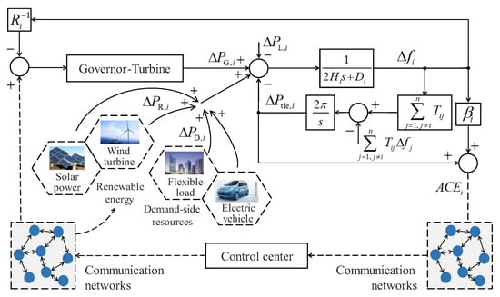
Figure 1.
The frequency control of an islanded microgrid with renewable energy stations, conventional generators, and demand-side resources.
It should be noted that Figure 1 represents a simplified framework of the islanded microgrid under extreme scenarios. First, regarding the communication network, part of the infrastructure may be destroyed during disasters. In this study, the remaining communication links are modeled with asynchronous and time-varying delays, which reflect the heterogeneous impacts of disrupted fiber-based and wireless-based channels. No additional redundancy or routing strategies are explicitly designed; instead, the focus is on ensuring that the proposed control method remains stable and robust in the presence of uncertain delays.
Second, with respect to electric vehicles (EVs), their contribution to frequency control via vehicle-to-grid (V2G) services depends on user willingness, which may be uncertain under emergency conditions. Here, EVs are modeled as controllable DSRs once they are connected to the grid and available for V2G. The variability of user participation is not explicitly represented, as the emphasis of this work is on the dynamic effects of asynchronous delays. Future research will consider incorporating communication redundancy, behavioral models, and incentive mechanisms to more comprehensively capture resilience aspects of communication networks and V2G participation under extreme conditions.
Taking a non-reheat thermal generating unit as an example, its frequency response dynamics can be expressed as [4]:
where is the control valve position deviation of the non-reheat unit, is the steam turbine time constant, is the speed droop coefficient of the governor, is the governor time constant, and is the control input of the non-reheat thermal unit.
In this study, the flexible resources in the power system are modeled as discrete-state flexible loads, which do not possess continuous dynamic processes. Their frequency regulation output corresponds to the change in power associated with a change in state.
Taking a squirrel-cage induction wind turbine generator as an example, the frequency dynamic characteristics of a renewable generating unit can be expressed as
where is the variation in the wind energy utilization coefficient of the wind turbine, is the variation in the pitch angle, is the variation in the tip speed ratio, is the variation in wind speed, is the air density, is the swept area of the turbine blades, is the variation in rotor angular velocity, is the synchronous angular velocity of the rotor, is the variation in the output power of the wind turbine, is the stator phase voltage, and are the rotor resistances, and are the stator and rotor reactances, respectively, and is the difference between the rotor angular velocity and its synchronous angular velocity.
The dynamic characteristics of the tie-line power can be expressed as
where denotes the synchronizing coefficient of the tie-line between area and area , satisfying ; represents the number of areas in the power system.
In power system frequency control, it is necessary not only to maintain the frequency stability of each area, but also to ensure that the tie-line power exchanges between control areas remain within reasonable limits. This control performance is characterized by the area control error (ACE), denoted as , which is defined as a linear combination of the frequency deviation and tie-line power deviation of area , namely:
where is the frequency bias factor of area iii in the power system, satisfying:
In conventional power system frequency control, the integral dynamics of the area control error are often introduced to form a proportional–integral (PI) feedback control strategy, which serves to reduce the steady-state error of frequency control, namely:
Due to the presence of response delays, the frequency regulation output functions of conventional generating units, wind turbine generators, and demand-side resources in the power system satisfy:
By selecting the frequency deviation , tie-line power deviation , output of the non-reheat thermal unit , control valve position deviation of the non-reheat unit , integral of the area control error , and wind turbine output as state variables, the state-space equations of the power system frequency dynamics—considering renewable plants, thermal units, and demand-side resources—can be constructed as:
where denotes the state variables; is the system control input; represents the source–load fluctuations; is the system output; denotes the system state matrix; denotes the system control matrix; represents the disturbance matrix; and denotes the system output matrix. The complete form of the system equations can be found in [4] and is therefore omitted here.
3. Frequency Control Method for Renewable-Dominated Power Systems Based on a Parametric Riccati Equation
It is noted that the power system frequency state-space Equation (13) involves asynchronous response delays, making it difficult to construct a conventional strict Lyapunov function. Therefore, a parametric Riccati equation is adopted to design a control strategy that is analytically tractable, tunable, and theoretically guaranteed. By introducing a positive parameter , the parametric Riccati equation can not only yield a positive-definite solution satisfying stability requirements but also flexibly adjust the convergence rate and control gains of the system, thereby enhancing the robustness of the power system frequency control against asynchronous response delays. In cases where it is impossible to construct a conventional strict Lyapunov function, it can be combined with a degenerate Lyapunov functional and Barbalat’s lemma to rigorously prove the global or semi-global asymptotic stability of the system.
Lemma 1 presents the controllability criterion for the power system frequency state-space Equations (13) and (14) considering asynchronous response delays.
Lemma 1
([27]). For the power system frequency state-space Equations (13) and (14) with asynchronous response delays, the system is completely controllable if and only if condition (15) holds.
Assume that the power system frequency control model (13)–(14) is completely controllable and observable. According to the properties of the system eigenvalues, the power system frequency state-space equations can be decomposed. By introducing a nonsingular matrix and the transformation , the power system frequency state-space equations can be equivalently rewritten as
where is the system matrix, is the control matrix, is the disturbance matrix, and is the output matrix such that
The eigenvalues of matrix lie in the left half-plane of the s-plane, while the eigenvalues of lie on the imaginary axis of the s-plane.
Theorem 1.
Consider the renewable energy power system frequency control Equations (17) and (18) with asynchronous response delays. When the source–load disturbance is zero, there exist a positive scalar and a control gain such that the closed-loop feedback system (19)–(21) based on PI control is asymptotically stable.
Proof.
Define the state observation error of the renewable energy power system frequency dynamic model as the difference between the actual state and the observed state , i.e.,
It is noted that the eigenvalues of the component of the state matrix lie in the left half-plane of the s-plane. Therefore, the system states coupled with are already asymptotically stable and do not require additional control measures. It is only necessary to focus on the stability of the following subsystem:
where
where is the difference between the state and the delayed state . The Lyapunov function for the renewable energy power system frequency dynamic model is defined as:
where the positive-definite matrix QQQ is the solution of the following algebraic equation.
The first derivative of the Lyapunov function with respect to time is given by:
We analyze the terms in one by one. Let denote the deviation between the state component and its delayed component ; then we have:
where , and is the upper bound of delay
Let
where is an arbitrary scalar greater than 1. Thus, for any , we have:
Thus, for , we have
Combining and , we obtain
Letting yields
Under the condition that holds, for any , the above equation can be rewritten as
where .
Substituting (37) and into yields
The second element in , , satisfies that
The third element in (29), , satisfies that
where
Substituting – into gives
Note that
We have
where is equal to .
For , we have
Thus, the proof of Theorem 1 is completed. □
Remark 1.
The influence of grid topology is reflected through the tie-line power exchange equations, which depend on the synchronizing coefficients of the interconnecting lines. A radial topology with fewer tie-lines results in weaker inter-area coupling and a lower algebraic connectivity of the Laplacian matrix, while a meshed topology provides stronger interconnections. These differences directly affect the area control error formulation and, consequently, the system’s frequency dynamics. To enhance performance under different topologies, the proposed parametric Riccati controller can be adapted by tuning the weighting matrix Q as a function of network connectivity, thereby increasing robustness for radial configurations and optimizing performance for meshed ones.
Remark 2.
PI controllers are robust but often conservative, while LQR controllers provide high performance under deterministic delays but degrade under uncertain conditions. Our proposed parametric Riccati equation-based method adaptively adjusts control gains, thereby maintaining transient performance while explicitly handling asynchronous, time-varying delays, striking a balance between robustness and optimality.
Remark 3.
The proposed controller advances the theory of frequency control by introducing a parametric Riccati equation framework that rigorously guarantees stability under asynchronous and time-varying delays, supported by a Lyapunov-Barbalat analysis. From a practical perspective, the method provides system operators with a control tool that adapts to heterogeneous communication delays without requiring detailed redesign for each scenario. This improves the reliability of renewable-dominated microgrids during extreme events where communication networks are partially degraded. The controller can be integrated into existing secondary frequency control architectures with minimal additional infrastructure, offering a feasible pathway to enhance grid resilience in practice.
Remark 4.
Note that (i) the current approach assumes perfect state observability, while sensor errors may affect practical performance, (ii) scalability to very large systems with hundreds of distributed resources may pose computational challenges, and (iii) the analysis is limited to frequency stability, without addressing voltage or power quality issues. Thus, future work will address observer design, scalable algorithms, and integrated stability metrics to overcome these limitations.
4. Case Study
In this section, a modified New England 39-bus power system is used as the test system. Four typical operating scenarios are considered: constant synchronous delay, constant asynchronous delay, time-varying synchronous delay, and time-varying asynchronous delay. The proposed output feedback control method is compared with the proportional–integral (PI) control method in [29] and the optimal control strategy based on the linear quadratic regulator (LQR) in [22]. Sensitivity analyses are also conducted to ultimately verify the effectiveness of the proposed control strategy.
All simulations were carried out on a desktop computer with an Intel Core i7-11700 CPU @ 2.50 GHz, 16 GB RAM, running Windows 11 (64-bit). The control algorithms and case studies were implemented in MATLAB/Simulink R2023b, with the Control System Toolbox and Simscape Power Systems toolbox. The dynamic equations were solved using the ode23tb solver with a step size of 0.001 s, and the total simulation horizon was set to 200 s for each scenario.
4.1. System Setting
In this section, a modified New England 39-bus power system is adopted as the test system for the case studies, with its single-line diagram shown in Figure 2. Relative to the conventional New England 39-bus system, the configuration in Figure 2 incorporates changes in both renewable energy integration and demand-side resource deployment. Specifically, wind farms are connected at buses 31 and 38, while flexible loads are installed at buses 37, 38, and 20. Area 1 comprises 500 demand-side resources, Area 2 comprises 1000, and Area 3 comprises 1500, each with a controllable power range of 1–2 kW. The parameters of the modified New England 39-bus system, the wind farms, and the demand-side resources are provided in [16]. The Simulink-based diagram of the modified IEEE 39-bus system is shown in Figure 3. This diagram describes the overall configuration of the system, where A1–A3 represent Areas 1–3 of the 39-bus system. The source–load fluctuations for Area 2 are illustrated in Figure 4.
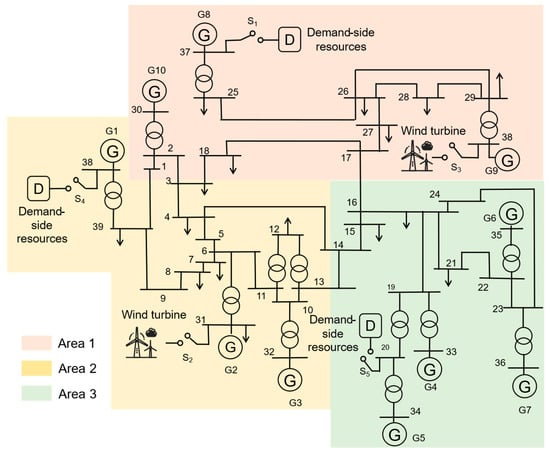
Figure 2.
The diagram of the modified New England 39 bus system.
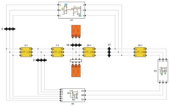
Figure 3.
The Simulink diagram of the test system.
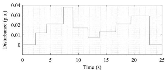
Figure 4.
Power and load fluctuations of power system in region 2.
The parameters of the IEEE 39-bus test system are summarized in Table 1, which lists the generator inertia constants, regulation parameters, damping coefficients, and turbine/generator time constants for the three interconnected areas [16].

Table 1.
Parameters of the 39-bus System [16].
To demonstrate the effectiveness of the proposed method, three approaches are considered for comparison, as described below.
Method 1: The proposed approach in this paper, which accounts for the impact of asynchronous and time-varying response delays on the frequency regulation output sequences of renewable energy plants, demand-side flexible resources, and conventional generating units. An output feedback frequency control strategy is designed based on a parameterized Riccati equation.
Method 2: The proportional–integral frequency control method proposed in [29], which models the response delay of demand-side flexible resources using the age-of-information concept from the communication domain. This method ignores the asynchrony of source–load response delays in power systems.
Method 3: The full-state feedback frequency control method based on the linear quadratic regulator (LQR) proposed in [22], which neglects the time-varying and asynchronous characteristics of delays. This approach requires state estimation using a state observer, for which a Kalman filter is adopted.
To characterize the features of response delays, four representative operating scenarios are considered:
Scenario 1: Constant synchronous delay. The response delays of renewable energy plants, demand-side flexible resources, and conventional generating units are all set to 0.4 s.
Scenario 2: Constant asynchronous delays. The response delays of renewable energy plants, demand-side flexible resources, and conventional generating units are set to 0.5 s, 0.8 s, and 0.3 s, respectively.
Scenario 3: Time-varying synchronous delay: The response delays of all three resource types are identical and time-varying, with the delay bounded within [0.1, 0.8] s.
Scenario 4: Time-varying asynchronous delays: The response delays are unequal and time-varying. The delay ranges are [0.1, 0.3] s for renewable energy plants, [0.3, 0.5] s for conventional generating units, and [0.5, 1.0] s for demand-side flexible resources.
4.2. Performance Analysis
Figure 5 illustrates the frequency responses of the power system under the four representative operating scenarios, where Figure 5a–d correspond to Scenarios 1–4, respectively. As shown in Figure 5a,b, in Scenarios 1 and 2, Method 3 yields frequency deviations closer to the steady-state frequency point (Δf = 0), with a smaller nadir and shorter settling time. This is because, under constant synchronous and constant asynchronous delays, the delays are deterministic. Moreover, Method 3 adopts a full-state feedback control strategy, providing richer state information than Methods 1 and 2, thereby achieving better frequency performance.
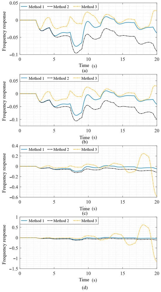
Figure 5.
Frequency response under scenarios 1~4. (a) Scenario 1. (b) Scenario 2. (c) Scenario 3. (d) Scenario 4.
In contrast, under Scenarios 3 and 4, Method 3 fails to maintain frequency stability in the presence of uncertain response delays. This is attributed to its focus on achieving optimal frequency performance under deterministic delays, at the expense of robustness under uncertain delays. By comparison, the proposed parameterized Riccati equation-based frequency control method for renewable-integrated power systems reduces the frequency nadir compared with Method 2 under constant delay conditions, and maintains frequency stability under time-varying delays, thus achieving a balance between dynamic performance and robustness.
4.3. Impacts of Parameteric Uncertainties
It is noted that both Method 1 and Method 2 are capable of maintaining frequency stability in the presence of time-varying delays. To further compare the frequency control performance of Methods 1 and 2, the impact of modeling errors is considered, i.e., the frequency dynamic model of the renewable-integrated power system in (17) is reformulated as follows:
where and represent the modeling errors of the power system frequency model. Larger values of and indicate greater parameter modeling errors in the power system.
The ranges of and are set to and , respectively. The source–load fluctuation is set to 0.04 p.u. Figure 6 shows the frequency nadirs corresponding to Methods 1 and 2.
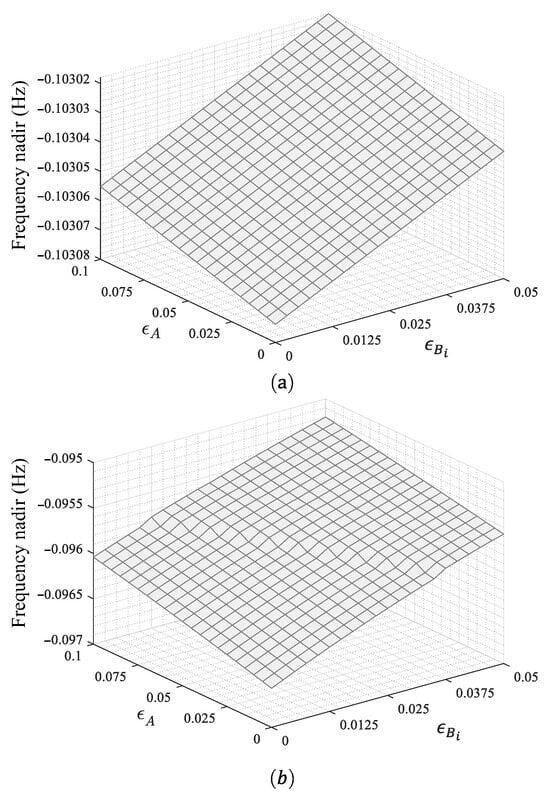
Figure 6.
Frequency nadir with different methods (a) Method 1. (b) Method 2.
As shown in Figure 6, the modeling errors and of the power system frequency model are strongly correlated with the system’s frequency performance. Specifically, as the modeling errors decrease, the absolute value of the frequency nadir increases, indicating a deterioration in the system’s transient frequency performance. Furthermore, a cross-comparison of the control performance of Methods 1 and 2 reveals that Method 1 exhibits a clear advantage in suppressing frequency decline. Compared with Method 2, Method 1 improves the control of the frequency nadir by 6.31–7.59%. This advantage arises from Method 1’s capability to incorporate delay information in adjusting the γ parameter of the parameterized Riccati equation, thereby formulating a more targeted frequency regulation strategy that effectively enhances the transient frequency performance of the power system.
4.4. Impacts of Communication Delay
Next, the impacts of the communication delay are analyzed. The power system response delay is increased from 0 s to 1.5 s, and the source–load fluctuation is set to 0.06 p.u. Figure 7 presents the system’s frequency performance under different response delays, including 0 s, 0.2 s, 1.0 s, and 1.5 s. As shown in Figure 7, with the proposed method, the frequency performance of the power system remains within a satisfactory range and does not exhibit a sudden degradation as the delay increases, indicating that the proposed method possesses strong robustness.
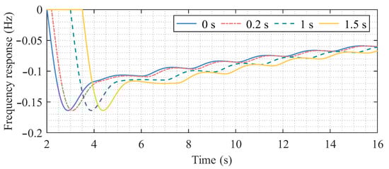
Figure 7.
Frequency response of the power system with the proposed method under various delays.
5. Conclusions
This paper addresses the challenge of balancing frequency robustness and transient performance in power systems when new energy power stations, conventional generators, and load-side resources jointly participate in frequency regulation. The issue arises from the asynchronous response delay among these resources. To solve this, we propose a novel frequency control method for new energy power systems based on a parameterized Riccati equation. This method uses adaptive adjustments of control parameters to strike a balance between system frequency robustness and optimality. First, we consider the frequency regulation capabilities of new energy power stations, conventional units, and load-side resources. We construct a power system frequency control model that accounts for asynchronous response delays by adjusting the response sequence of these diverse resources. Next, based on Barbalat’s lemma, we introduce a new frequency control method for new energy power systems using a parameterized Riccati equation. Finally, the effectiveness of the proposed method is validated through tests on a modified New England 39-bus system.
Despite its contributions, this study has several limitations. First, communication resilience is represented only through asynchronous and time-varying delay modeling; complete interruptions and redundancy mechanisms are not explicitly considered. Second, electric vehicles are modeled as controllable demand-side resources once they are connected, without accounting for uncertainties in user willingness to participate in V2G services during emergencies. Third, the proposed control method relies on a linearized state-space model and has been validated on a modified New England 39-bus system; further validation on larger systems and real-time hardware-in-the-loop platforms is still needed. These limitations highlight important directions for future work, including the integration of communication resilience mechanisms, behavioral models of user participation, and experimental validations in more realistic environments. Additionally, we can also investigate the energy hub operation under uncertainty [30] and for advanced cyber-resilience strategies for frequency control [31].
Author Contributions
Conceptualization, J.G. and C.S.; methodology, L.L. and H.Z.; software, J.G. and H.Z.; validation, J.G., C.S. and Y.Z.; formal analysis, C.L.; investigation, C.S.; resources, J.G.; data curation, L.L.; writing—original draft preparation, J.G.; writing—review and editing, J.G. All authors have read and agreed to the published version of the manuscript.
Funding
This research was funded by National Natural Science Foundations of China (52477074, 524B2101) and National Key Research and Development Program of China (No. 2023YFA1011304).
Institutional Review Board Statement
Not applicable.
Informed Consent Statement
Not applicable.
Data Availability Statement
Data are available upon request.
Acknowledgments
We would like to express our sincere gratitude to the anonymous reviewers for their invaluable time, insightful comments, and constructive suggestions on our manuscript.
Conflicts of Interest
Jijiang Gu has received research grants from Guangxi Electric Power Company. Ling Li and Yangjun Zhou has received research grants from Guangxi Key Laboratory of Intelligent Control and Maintenance of Power Equipment. Changzheng Shao, Hanxin Zhang, and Chengrong Lin have received research grants from NSFC. The authors declare no conflicts of interests.
Correction Statement
This article has been republished with a minor correction to the Funding statement. This change does not affect the scientific content of the article.
References
- Kasimalla, S.R.; Park, K.; Zaboli, A.; Hong, Y.; Choi, S.L.; Hong, J. An evaluation of sustainable power system resilience in the face of severe weather conditions and climate changes: A comprehensive review of current advances. Sustainability 2024, 16, 3047. [Google Scholar] [CrossRef]
- Ward, L.; Subburaj, A.; Demir, A.; Chamana, M.; Bayne, S.B. Analysis of grid-forming inverter controls for grid-connected and islanded microgrid integration. Sustainability 2024, 16, 2148. [Google Scholar] [CrossRef]
- Ottenburger, S.S.; Cox, R.; Chowdhury, B.H.; Trybushnyi, D.; Omar, E.A.; Kaloti, S.A.; Ufer, U.; Poganietz, W.R.; Liu, W.; Deines, E.; et al. Sustainable urban transformations based on integrated microgrid designs. Nat. Sustain. 2024, 7, 1067–1079. [Google Scholar] [CrossRef]
- International Energy Agency (IEA). Renewables 2024: Analysis and Forecast to 2030; IEA: Paris, France, 2024; Available online: https://www.iea.org/reports/renewables-2024 (accessed on 16 September 2025).
- European Commission. Stepping up Europe’s 2030 Climate Ambition: Investing in a Climate-Neutral Future for the Benefit of Our People; European Commission: Brussels, Belgium, 2020.
- National Energy Administration of China (NEA). China Renewable Energy Development Report 2023; NEA: Beijing, China, 2023.
- U.S. Department of Energy (DOE). The Long-Term Strategy of the United States: Pathways to Net-Zero Greenhouse Gas Emissions by 2050; DOE: Washington, DC, USA, 2021.
- ENTSO-E. Network Code on Load-Frequency Control and Reserves (NC LFC&R); Network of Transmission System Operators for Electricity: Brussels, Belgium, 2013. [Google Scholar]
- Kerdphol, T.; Rahman, F.S.; Mitani, Y.; Hongesombut, K.; Küfeoğlu, S. Virtual inertia control-based model predictive control for microgrid frequency stabilization considering high renewable energy integration. Sustainability 2017, 9, 773. [Google Scholar] [CrossRef]
- Sahu, P.R.; Lenka, R.K.; Khadanga, R.K.; Hota, P.K.; Panda, S.; Ustun, T.S. Power system stability improvement of facts controller and pss design: A time-delay approach. Sustainability 2022, 14, 14649. [Google Scholar] [CrossRef]
- Khalil, A.; Rajab, Z.; Alfergani, A.; Mohamed, O. The impact of the time delay on the load frequency control system in microgrid with plug-in-electric vehicles. Sustain. Cities Soc. 2017, 35, 365–377. [Google Scholar] [CrossRef]
- Yan, R.; Saha, T.K.; Bai, F.; Gu, H. The anatomy of the 2016 south australia blackout: A catastrophic event in a high renewable network. IEEE Trans. Power Syst. 2018, 33, 5374–5388. [Google Scholar] [CrossRef]
- Haes Alhelou, H.; Hamedani-Golshan, M.E.; Njenda, T.C.; Siano, P. A survey on power system blackout and cascading events: Research motivations and challenges. Energies 2019, 12, 682. [Google Scholar] [CrossRef]
- Dreidy, M.; Mokhlis, H.; Mekhilef, S. Inertia response and frequency control techniques for renewable energy sources: A review. Renew. Sustain. Energy Rev. 2017, 69, 144–155. [Google Scholar] [CrossRef]
- Alayi, R.; Zishan, F.; Seyednouri, S.R.; Kumar, R.; Ahmadi, M.H.; Sharifpur, M. Optimal load frequency control of island microgrids via a pid controller in the presence of wind turbine and pv. Sustainability 2021, 13, 10728. [Google Scholar] [CrossRef]
- Elkasem, A.H.; Khamies, M.; Hassan, M.H.; Nasrat, L.; Kamel, S. Utilizing controlled plug-in electric vehicles to improve hybrid power grid frequency regulation considering high renewable energy penetration. Int. J. Electr. Power Energy Syst. 2023, 152, 109251. [Google Scholar] [CrossRef]
- Ta, V.Q.; Park, M. MAN-EDoS: A multihead attention network for the detection of economic denial of sustainability attacks. Electronics 2021, 10, 2500. [Google Scholar] [CrossRef]
- Badesa, L.; Teng, F.; Strbac, G. Conditions for regional frequency stability in power system scheduling—Part ii: Application to unit commitment. IEEE Trans. Power Syst. 2021, 36, 5567–5577. [Google Scholar] [CrossRef]
- Hao, H.; Sanandaji, B.M.; Poolla, K.; Vincent, T.L. Aggregate flexibility of thermostatically controlled loads. IEEE Trans. Power Syst. 2014, 30, 189–198. [Google Scholar] [CrossRef]
- Williams, B.; Bishop, D.; Gallardo, P.; Chase, J.G. Demand side management in industrial, commercial, and residential sectors: A review of constraints and considerations. Energies 2023, 16, 5155. [Google Scholar] [CrossRef]
- Lin, C.; Hu, B.; Shao, C.; Xie, K.; Peng, J.C.H. Computation offloading for cloud-edge collaborative virtual power plant frequency regulation service. IEEE Trans. Smart Grid 2024, 15, 5232–5244. [Google Scholar] [CrossRef]
- Pourmousavi, S.A.; Nehrir, M.H. Introducing dynamic demand response in the LFC model. IEEE Trans. Power Syst. 2014, 29, 1562–1572. [Google Scholar] [CrossRef]
- Hu, Z.; Zhang, K.; Su, R.; Wang, R. Robust cooperative load frequency control for enhancing wind energy integration in multi-area power systems. IEEE Trans. Autom. Sci. Eng. 2024, 22, 1508–1518. [Google Scholar] [CrossRef]
- Huang, X.; Fan, Y.; Wu, H.; Zhang, G.; Yin, Z.; Khan, M.Y.A.; Liu, H.; Zhai, J. Distributed secondary control for islanded microgrids considering communication delays. IEEE Access 2024, 12, 64335–64350. [Google Scholar] [CrossRef]
- Sun, J.; Tan, S.; Zheng, H.; Qi, G.; Tan, S.; Peng, D.; Guerrero, J.M. A dos attack-resilient grid frequency regulation scheme via adaptive v2g capacity-based integral sliding mode control. IEEE Trans. Smart Grid 2023, 14, 3046–3057. [Google Scholar] [CrossRef]
- Qiao, S.; Liu, X.; Wang, Y.; Xiao, G.; Wang, P. H∞ load frequency control of power system integrated with evs under dos attacks: Non-fragile output sliding mode control approach. IEEE Trans. Intell. Transp. Syst. 2024, 25, 4565–4577. [Google Scholar] [CrossRef]
- Richard, J.P. Time-delay systems: An overview of some recent advances and open problems. Automatica 2003, 39, 1667–1694. [Google Scholar] [CrossRef]
- Shangguan, X.C.; Zhang, C.K.; He, Y.; Jin, L.; Jiang, L.; Spencer, J.W.; Wu, M. Robust load frequency control for power system considering transmission delay and sampling period. IEEE Trans. Ind. Inform. 2021, 17, 5292–5303. [Google Scholar] [CrossRef]
- Jiao, D.; Shao, C.; Hu, B.; Xie, K.; Lin, C.; Ju, Z. Age-of-information-aware PI controller for load frequency control. Prot. Control Mod. Power Syst. 2023, 8, 39. [Google Scholar] [CrossRef]
- Giannelos, S.; Pudjianto, D.; Zhang, T.; Strbac, G. Energy hub operation under uncertainty: Monte Carlo risk assessment using gaussian and KDE-based data. Energies 2025, 18, 1712. [Google Scholar] [CrossRef]
- Oshnoei, S.; Mahboubi-Moghaddam, E.; Khooban, M.H. Advanced defense strategy for cyber-resilient frequency control in real power grids. IEEE Trans. Autom. Sci. Eng. 2025, 22, 19366–19376. [Google Scholar] [CrossRef]
Disclaimer/Publisher’s Note: The statements, opinions and data contained in all publications are solely those of the individual author(s) and contributor(s) and not of MDPI and/or the editor(s). MDPI and/or the editor(s) disclaim responsibility for any injury to people or property resulting from any ideas, methods, instructions or products referred to in the content. |
© 2025 by the authors. Licensee MDPI, Basel, Switzerland. This article is an open access article distributed under the terms and conditions of the Creative Commons Attribution (CC BY) license (https://creativecommons.org/licenses/by/4.0/).