Article

Predicting the Performance of a Helically Coiled Heat Exchanger for Heat Recovery from a Waste Biomass Incineration System

by
Izabela Wardach-Świȩcicka
1,*,
Sylwia Polesek-Karczewska
1 and
Adam Da̧browski
2
1
Institute of Fluid-Flow Machinery, Polish Academy of Sciences, Fiszera 14 St., PL 80-231 Gdansk, Poland
2
PW “En-Tech” Adam Da̧browski, Zielona 1 St., PL 84-252 Orle, Poland
*
Author to whom correspondence should be addressed.
Sustainability 2025, 17(2), 759; https://doi.org/10.3390/su17020759
Submission received: 6 December 2024 / Revised: 8 January 2025 / Accepted: 16 January 2025 / Published: 19 January 2025
(This article belongs to the Special Issue Thermally Driven Renewable Energy Technologies)

Abstract

Nowadays, with increasing concerns about the environment and energy security, efforts have intensified to develop effective energy generation technologies based on renewable sources that align with the principles of sustainable growth. In response to these demands, biomass-fueled furnaces have become essential components of modern combined heat and power generation systems. This work aims to predict the thermal performance of a helically coiled multi-tube heat exchanger designed to recover heat from waste biomass incineration flue gases. The working fluid used is thermal oil. The work focuses on determining the thermal output of a heat exchanger for prescribed design parameters, including the thermal parameters of cooling oil and the temperature difference of flue gas, and the geometrical details. A novel in-house stationary lumped multi-section model, utilizing the iterative calculation method, was developed, allowing fast predictions of the operation parameters of helically coiled multi-tube type heat exchangers. Two different configurations of the exchanger, three-pipe (case I) and four-pipe (case II), were considered. The thermal output obtained from calculations for case I showed a satisfactory convergence with the value based on the measurement data, at about 6%. Once validated, the model was used to determine the required heat exchange surface area of a four-pipe heat exchanger of larger design heat output (2.2 MW) and assumed tube dimensions and configurations. The accuracy of the heat exchanger capacity prediction was below 12%, proving the developed calculation tool to be reliable for design and optimization purposes.

1. Introduction

At the core of sustainable economic development worldwide is the pressing need to reduce energy consumption and transition from fossil fuels to renewable energy sources. These priorities have driven intensified efforts to develop efficient energy conversion systems, including new units and adaptations of existing ones, to be fueled by various kinds of solid fuels, including low-grade biogenic materials [1,2]. This, in particular, applies to small-scale combined heat and power units, underpinning distributed energy systems fed by locally available resources [3]. Thermally efficient heat exchangers as the basic components of such systems largely contribute to their efficiency [4,5,6,7], and thereby reducing the fuel consumption and leading to overall energy savings that lie behind the economic and society sustainability goals. Therefore, much of the research in this area focuses on heat transfer enhancement [8].
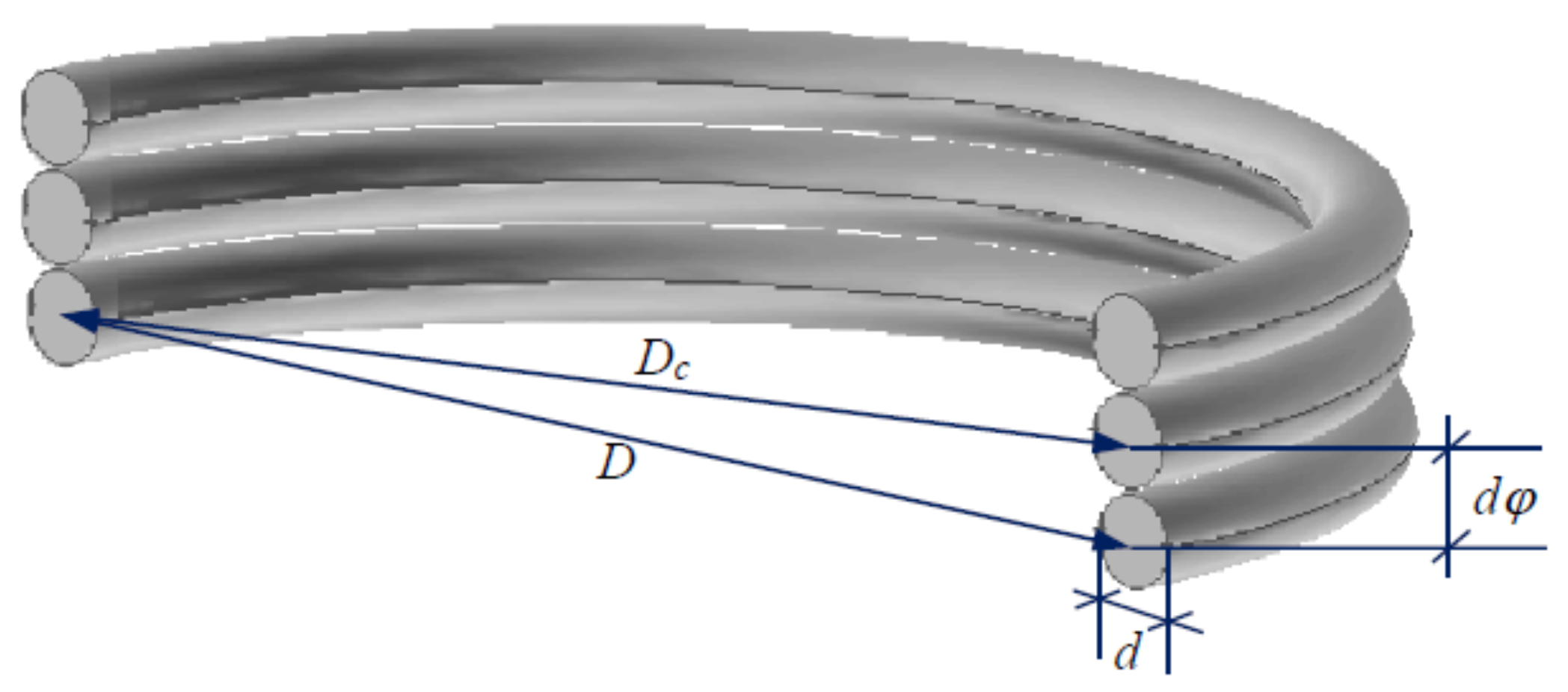
Helically coiled tubes are considered to be among the most beneficial solutions for thermal units since they offer high heat transfer rates, higher compared to straight tubes, particularly in the case of laminar flows [9,10]. With this, they feature not only higher effectiveness than other tube-type heat exchanger geometries but also large heat exchange surface area-to-volume ratios that translate into their compactness. Owing to these features, they have been widely used for decades in various industrial applications, such as heat recovery systems [11,12], thermal energy storage systems [13], refrigeration and air conditioning installations [14,15,16], as well as chemical and food industry [17].
There are numerous works available devoted to the analysis of thermal and flow characteristics of helically coiled type heat exchangers, including both experimental examination and numerical calculations. The latter are essential since the performance of a heat exchanger is always a question of the thermophysical properties of working fluids, the exchanger design, as well as the enhancement technique to be used, either active or passive. Considering the time and cost involved in the experimental work, calculations can considerably improve the design and optimization of these devices.
In the literature, two basic methods of thermal calculations for various types of heat exchangers can be found [18]. The first one utilizes the logarithmic mean temperature difference (LMTD), and the second is the so-called ϵ -NTU method (where ϵ means the heat exchanger effectiveness and NTU is the number of heat transfer units). Both methods are based on steady-state conditions and the energy balance equation between hot and cold fluids. The ϵ -NTU method is particularly helpful when the outlet temperatures of the fluids are not known. It assumes constant heat transfer coefficient and fluid properties, which in the case of thermal oil and complex geometry of the system can give unreasonable results, burdened with an error [19]. The LMTD method is used if all inlet and outlet temperatures are known and the unknown is the required heat transfer area. This approach eliminates the need for iterative calculations, making it computationally efficient. Furthermore, it assumes that the outlet temperatures of both fluids are already known. If they are not, an iterative procedure is needed, which can complicate the analysis. Similarly to the ϵ -NTU method, in this one, the constant properties are often assumed, which may not hold for systems with large temperature variations [20].
Various researchers utilize CFD tools to analyze the effects of different factors, such as flow rate and geometrical parameters on the performance of heat exchangers. Tuncer et al. [21] used CFD to simulate heat transfer and fluid flow inside the shell and helically coiled tube in two configurations, conventional and modified aiming at achieving an exchanger of improved efficiency. Omidi et al. [22] carried out CFD analysis on flow characteristics and heat transfer in a helical coil with four different lobed cross sections, focusing on the impact of the lobe number, coil diameter, flow parameters, as well as nanoparticles on the performance of a heat exchanger. Abu-Hamdeh et al. [23] performed CFD simulations to examine heat transfer and pressure drop in the new type helically coiled tube heat exchangers (type named “sector-by-sector”), and the helical coiled tube-in-tube heat exchanges for comparison. In another work, Abu-Hamdeh et al. [24] using CFD approach investigated the thermal-hydraulic characteristics of a helical micro double-tube heat exchanger, considering configurations with various pitch lengths and number of turns. Recently, Elsaid et al. [25] studied numerically the thermal-hydraulic performance of the shell and helically coiled tube heat exchanger, covering various tube cross-sections (circular, elliptic, and square). Similar cross-section geometries of coiled tubes were also investigated using CFD calculations by Kurnia et al. [26], who aimed at evaluating heat transfer performance and entropy generation of laminar flow in the hellically coiled tube under heating and cooling. Haskinks and El-Genk [27] used CFD to analyze friction pressure losses on the shell side of annular heat exchangers with the concentric helically coiled tubes, considering isothermal flows of liquid sodium, water, and helium gas. The simulation cases involved different HEX configurations, with the number of coils varying from 4 to 16, arriving at the total computation time of order of days, depending on the numerical mesh grid refinement.
It is noteworthy that advanced CFD simulations might be challenging for complex heat exchanger geometry, and time-consuming, and therefore may not be effective in practical use [28]. The literature review shows the lack of studies related to thermal analysis of helically coiled tube heat exchangers in small and medium-scale units that utilize in-house codes for fast predictions of an exchanger performance serving as a useful tool in the design and verification of preliminary geometry.
Soni and Chiesa [29] developed a calculation code aimed at the thermal rating of helically coiled heat recovery boilers with parallel coaxial coils fed with flue gases parallelly in a counterflow. Their program is based on a one-dimensional model, allowing the computational domain to be divided longitudinally into subsections to account for geometrical variations. Andrzejczyk and Muszyński [30] carried out the NTU-based calculations and designed a single-tube helically coiled heat exchanger to eventually experimentally verify the influence of external tube surface modification on the heat transfer coefficient. The authors’ study involved both, the co-current and counter-current, flow configuration. Alimoradi [31] studied the effect of operational and geometrical parameters on the thermal effectiveness of shell-and-helically coiled tube heat exchangers under steady state. Based on the experimentally validated simulation data on heat transfer in the heat exchanger, he carried out calculations of effectiveness and NTU. Employing the NTU analysis, Panahi and Zamzamian [32] studied the performance of a shell-and-coiled tube heat exchanger with helical wire inserted as a turbulator. In their investigation, the authors aimed to determine the thermal and frictional performance of the designed exchanger compared to the one without the turbulizing wire. Mirgolbabaei [33] investigated the thermal performance of vertical helically coiled heat exchangers of different geometrical parameters, including coil pitch and tube diameter, through CFD simulation and ϵ -NTU analysis. Unlike the most common approaches that involve constant temperature or heat flux at the tube wall, he implemented a conjugate boundary condition (a fluid-to-fluid heat transfer), arriving at reasonable predictions for the studied configuration. The authors of the present work, in their previous study [34], proposed the stationary lumped-cell model to simulate the thermal characteristics of the domestic biomass boiler with an integrated helically coiled tube heat exchanger cooled with thermal oil, designed to operate with the organic Rankine cycle (ORC) power generation system. Good agreement between the calculation results and measurement data was obtained, proving the approach to be reliable in estimating the thermal performance of the helically multi-coiled exchangers.
The goal of this study is to utilize the numerical approach based on a one-dimensional lumped-cell model, similar to the one previously developed, to analyze the thermal performance of a helically coiled multi-tube heat exchanger designed to recover heat from waste biomass combustion flue gases. The calculation results for the three-pipe heat exchanger of heat output of 1.2 MW were validated with the measurements. Next, the calculations were performed to examine the thermal and flow characteristics of a four-pipe exchanger to be designed and determine the required heat exchange surface area for the assumed heat output of 2.2 MW.

2. Heat Exchanger Performance Calculations

The study considers a coiled oil heating multi-tube heat exchanger, designed to utilize the heat from waste biomass incineration. The scheme and the real view of such a heat unit is presented in Figure 1 [35,36].
A unified mathematical model for the energy balance of the multi-coil system was used to predict thermal-flow parameters for this special heater designing issues. An in-house numerical code [34] was chosen for the calculations that were carried out in two steps:
  • step I, which involved the calculations for the three-pipe helically coiled heat exchanger (HCHE) of a designed thermal capacity of 1.2 MW and validation of the predictions with measurement data,
  • step II, wherein the calculations aimed at predicting the thermal and flow characteristics of a four-pipe HCHE of the assumed thermal output of 2.2 MW, to eventually determine the required heat exchange surface area.

2.1. Methodology—In-House Numerical Procedure

A unified mathematical model for the energy balance of the multi-coil system was developed and implemented using FORTRAN90 code. The details of such solutions are presented in the authors’ previous work [34]. For a better understanding, the basic equations and assumptions are given below. The model postulates that each control volume encompasses the paired hot fluid flow section flue gas and the tube with the internal cold fluid flow (thermal oil).
The two-equation system, involving mass and energy conservation, for the hot and cold sides is considered for each numerical cell. Figure 2 shows the energy balance for the i-th cell, representing the single coil segment of a studied heat exchanger (Figure 1—left picture). The energy balance for the hot side takes into account five thermal fluxes representing the following:
  • Energy of inflow stream Q ˙ H , i ;
  • Energy of outflow stream Q ˙ H , i o u t ;
  • Energy of chemical reactions Q ˙ H c h i ;
  • Thermal radiation of gas volume Q ˙ H r a d i ;
  • Convection heat transfer between gas and the tube surface Q ˙ H c o n v i .
Similarly, the cooling flow side considers four fluxes:
  • Energy of inflow stream Q ˙ C , i i n ;
  • Energy of outflow stream Q ˙ C , i o u t ;
  • Wall radiation Q ˙ C r a d i ;
  • Wall-to-liquid convection Q ˙ C c o n v i .
The set of governing equations for the system are presented below. They include mass and energy conservation equations for both the hot and cold sides.
For gas stream:
m ˙ H , i i n + Γ ˙ i m ˙ H , i o u t = 0 ,
Q ˙ H , i i n Q ˙ H , i o u t + Q ˙ H c h i Q ˙ H r a d i Q ˙ H c o n v i = 0 .
For liquid stream:
m ˙ C , i i n m ˙ C , i o u t = 0 ,
Q ˙ C , i i n Q ˙ C , i o u t + Q ˙ C r a d i + Q ˙ C c o n v i = 0 .
The particular terms of the above equations are summarized in Table 1.
The parameter Γ i ˙ in Equation (1) represents the gas mass source due to fuel combustion (heat source for the hot medium). This is assumed to take place only in the first cell i = 0 , which gives the following condition for other cells:
Γ ˙ i = 0 for i 0 .
The wall temperature ( T w a l l ) is defined based on the heat balance between the hot and cold medium:
m ˙ H c p , H T H T w a l l = m ˙ C c p , C T w a l l T C ,
which gives
T w a l l = G T H + T C 1 + G , G = m ˙ H c p , H m ˙ C c p , C .
Quantity ε w a l l in Equation (2d) stands for the effective emissivity of the tube wall given as ε w a l l = ε w a l l + 1 / 2 , where ε w a l l is the wall emissivity.
The mathematical procedure requires the determination of the heat exchange surface area (A, see Table 1). Owing to the specific design of the heat exchanger affecting the flow characteristics, an effective heat transfer surface area should be accounted for. Based on the additionally carried out 2D CFD simulation of gas flow over the number of coils, the effective surface ( A e f f ) was estimated at the level of 30–40% of the total coil lateral surface [34], depending on the tube diameter.
The studied problem leads to the solution of two-equation system (Equations (2) and (4)) with unknown temperatures T H , i i n , T H , i o u t , T C , i i n and T C , i o u t . It is noteworthy that the form of radiation heat fluxes, i.e., the fourth power of temperature (see Equations (2d) and (4c)), makes the equation system non-linear. To initialize the solution, the inlet temperature values have to be set, and the output parameters are then determined iteratively. The Newton method was used [37] to solve the given non-linear problem.
It should be added that flow phenomena in helical tubes, or curved tubes in general, are far more complex than that in straight tubes, and the pressure drops reported for the helical tubes are found to be higher compared to the flow through straight tubes [38]. However, the analysis of pressure drop remains an issue in itself, since it is affected by many factors, basically geometry-related [10]. The present study is limited to the analysis of thermal performance, but to obtain the full thermal and flow characteristics of the exchanger, the code can be extended to include the correlations for estimation of pressure drop. This would involve the advanced CFD flow analysis or/and the utilization of data/correlations available in the literature [39].

2.2. Physico-Chemical Properties

As mentioned, the flue gas fed to the heat exchanger is derived from the combustion of waste biomass. The ultimate and proximate analyses of the fuel considered are summarized in Table 2. For the purpose of the present study, own measurement data on the chemical composition (CHNS) of wood pellets were adopted [40]. These data are used only to determine the adiabatic combustion temperature of the fuel and the resulting temperature of flue gas fed to the heat exchanger. The chemical analysis does not include an ash composition which is responsible for the deposits on the exchanger tubes. It shall be noted that this study focuses only on a rough estimate of the required heat transfer surface area. Having regard to possible deposit agglomeration and slagging on the tube’s outer surface and related decrease in heat transfer coefficient, the design value of the heat exchange surface is usually taken at least 15% larger than the one predicted.
Based on the input mass flow rates of air and fuel, the excess-air ratio is estimated, which is expressed as [41,42]:
λ = 1 λ s * m ˙ a i r i n m ˙ f u e l i n ,
where λ s * is the stoichiometric air-to-fuel mass ratio determined from the ultimate analysis.
The temperature of flue gas fed to the heat exchanger was assumed to be adiabatic and iteratively computed from the equation:
Q ˙ H i n + Q ˙ c h = Q ˙ H o u t ,
which is further written as
m ˙ H i n c p , H T H T H i n + Γ ˙ · H H V = m ˙ H i n + Γ ˙ c p , H T a d T a d + Q ˙ l o s s ,
where term Q ˙ l o s s represents the losses due to inefficient combustion and non-ideal insulation. The flue gas is a mixture of fixed composition, and its specific heat is evaluated using the NASA polynomials formula [43]:
c p ( T ) = a T 2 + b T + c + d T + e T 2 + f T 3 + g T 4 M ¯ m i x , kJ / kgK ,
where M ¯ m i x is a mixture molar mass. The values of coefficients ag are calculated as a simple mole fraction average, i.e., a = j a j X j with the sum over the number of mixture compounds. The respective coefficients are provided in Table 3. The mixture thermal conductivity required for the heat transfer coefficient determination is defined by the chemical composition and temperature [34].
The tabulated data for air adapted from [44] were used to determine the hot gas dynamic viscosity. The Clapeyron relation was utilized to obtain temperature-dependent gas density:
ϱ H = p R i n d T , kg / m 3 ,
where R i n d is the individual gas constant for mixture, whereas p denotes pressure. For thermal oil properties, including density, specific heat and thermal conductivity, the linear temperature-dependent functions (for temperature in K) were adopted, respectively [45]:
ϱ C = 0.650 T + 1053.589 , kg / m 3 ,
c p , C = 3.594 T + 830.934 , J / ( kg K ) ,
λ C = 0.0001 T + 0.1555 , W / ( m K )
The kinematic viscosity of thermal oil was described by power-type relationship:
ν C = a 1 T + b 1 , m 2 / s for T 313 K a 2 T b 2 , m 2 / s for T > 313 K ,
with coefficients a 1 , b 1 , a 2 , b 2 determined based on the manufacturer’s data [46].

2.2.1. Convective Heat Transfer

Flow characteristics and, consequently, the convection, strongly depends on geometry. The latter, in the case of helically coiled tube heat exchangers, is as aforementioned, complex. A cutout of a helical coil is schematically shown in Figure 3. The diameter of curvature D c for j-th coil is defined as:
D c = d φ 2 / 4 + D 2 ,
where D is the coiled tube annulus diameter and d φ denotes the coil pitch. For the purpose of this study, the tube is assumed to be thin-walled. The single coil segment length is thus expressed as:
L = π d φ 2 + D 2 ,
In general, the heat transfer coefficient is a function of flow characteristics, defined by the Nusselt number, the thermal conductivity of the flowing fluid λ , and the characteristic flow dimension d, according to the relationship:
α = N u λ d , N u = f ( R e , P r ) .
Obviously, the characteristic dimension for oil flow is the tube diameter, while for flue gas flow it is the equivalent diameter. To determine the heat transfer coefficient on the exhaust gas-side α H , the Nusselt number defined by Reiher and Hilpert correlation for a single pipe in a cross-flow was utilized:
N u H = C R e n
with coefficients C and n dependent on Reynolds number [47]. The gas velocity characterizing the R e is expressed as
v H = m ˙ H A H ϱ H ,
where A H is the cross-sectional area for gas flow.
For the cold-side flow (tube), the Nusselt number is defined through the inner-diameter d and length L, and described by the following relationships [47,48]:
For laminar flow ( R e < 2100 ):
N u C = 1.86 μ μ w a l l 0.14 R e P r d L 1 / 3 for R e P r d L > 13 0.5 R e P r d L for R e P r d L < 4.5 ,
for fully developed turbulent flow ( R e > 10 4 ):
N u C = 0.027 μ μ w a l l 0.14 R e 0.8 P r 1 / 3 ,
and for the transition region ( 2100 R e 10 4 ):
N u C = 6.9 × 10 4 R e 1.24 P r 0.5 ,
with μ denoting dynamic viscosity calculated for an average medium temperature, and μ w a l l referring to the value determined at the wall temperature. Additionally, the correction for heat transfer coefficient accounting for the tube curvature was considered [41]:
α = α 0 1 + 3.54 d D c ,
where α 0 represents the heat transfer coefficient for the straight tube.

2.2.2. Gas Radiation

The radiative properties of flue gases, emissivity ε H , and absorptivity a H , are calculated considering the contents of radiating gas components, such as CO 2 and H 2 O , according to:
ε H = ε CO 2 + β ε ε H 2 O ε CO 2 β ε ε H 2 O
and
a H = ε CO 2 T H T w a l l 0.65 + β ε H 2 O Δ ε H ,
where β is the correction factor for increased steam concentration in flue gases and Δ ε H is the correction factor related to the mutual energy absorption emitted by different radiating gas components [47,48]. Quantity β ε represents the correction factor representing the influence of water steam pressure:
β ε = 1 + 0.6225 0.1346 ln p H 2 O L z 1 kPa · m p H 2 O 100 kPa ,
where L z represents the semi-circle radiating gas volume L z = 4 V / S , where V and S denote the volume and the total outer surface of the gas volume, respectively. Both radiating components’ emissivity values were determined based on Hottel’s graphs [47,48].

3. Results

3.1. Step I—Three-Pipe HCHE Case

The developed calculation method was first applied to the real test case of the HCHE composed of three tube coils. It is assumed that each of them consists of different numbers of coil segments, as is presented in Table 4. The table includes the input computation parameters, i.e., the geometry dimensions, media mass flow rates, the oil temperature at the HE outlet and the flue gas composition.
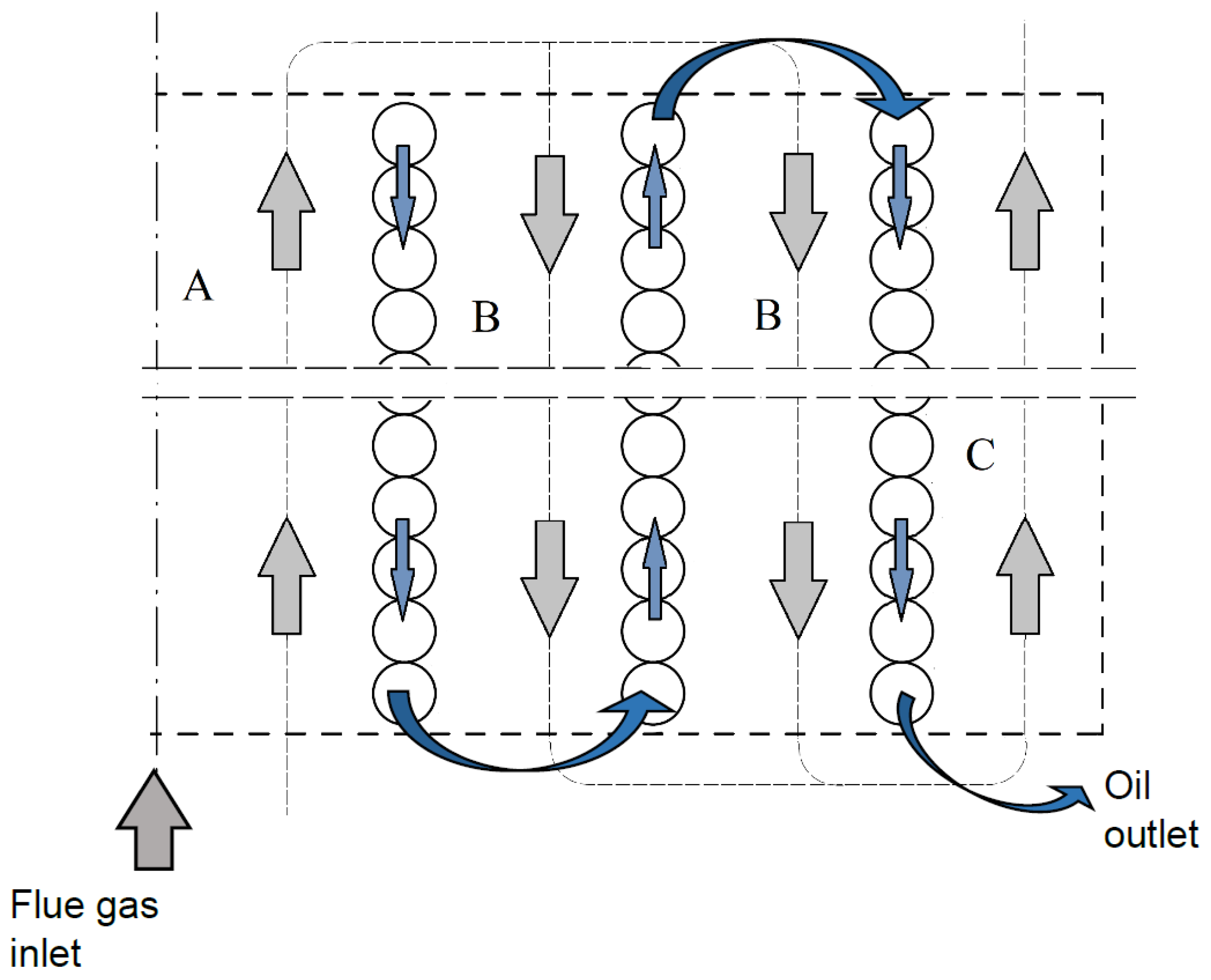
The half cross-sectional view of the exchanger, showing the flow directions of the hot fluid (flue gas) and the cold fluid (thermal oil), is schematically displayed in Figure 4. As shown in the figure, due to the differing flow characteristics across the specific sections of the heat exchanger, the heat exchanger volume was divided into three general zones for calculation purposes:
  • zone A—flue gas flow in the inner coil core,
  • zone B—covering flue gas annular flow in the volume between the inner and outer coil,
  • zone C—comprising flue gas annular flow in the volume between the outer coil and the wall.
Following such an approach, a heat exchanger is considered a counterflow type.
To check whether the required thermal output of the heat exchanger is obtained, the calculations utilize the mass flow rates of fluids and the inlet flue gas temperature (see values with star, shown in Table 4). It shall be mentioned that the flow rate of flue gas is a value resulting from the general thermal balance for given oil parameters and assumed inlet/outlet temperature difference on the hot side.
The physical properties of Therminol 66 ([45]) were adopted for calculations. The composition of flue gas, presented in Table 4, was determined based on the global reaction of the fuel combustion, given its chemical composition.
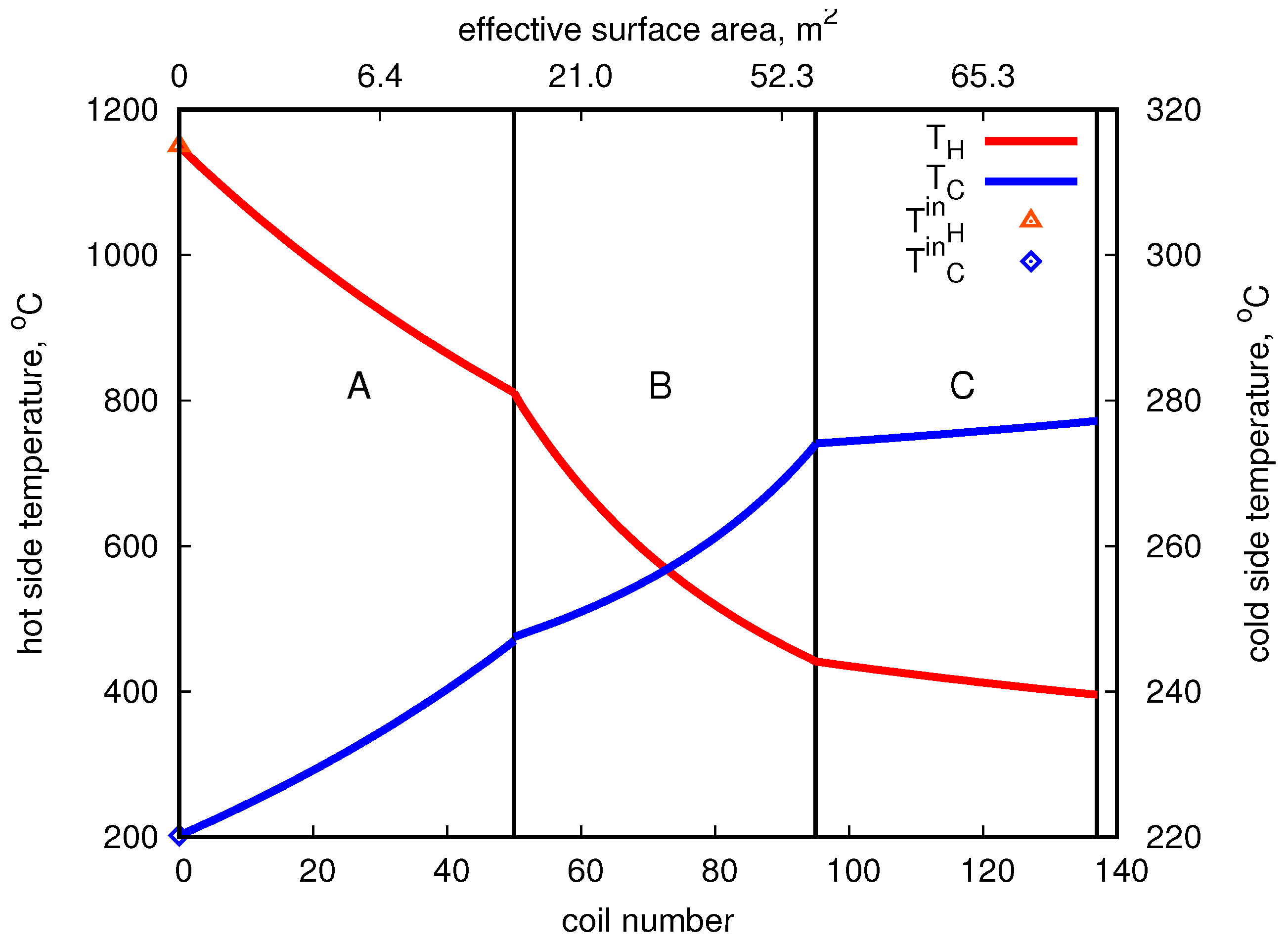
The flue gas temperature at the inlet to the heat exchanger was assumed adiabatic, T H i n = T a d , which equals approximately 1150 °C. Additionally, the outlet oil temperature T C o u t was set to the upper limit of 280 °C. The lower limit for the outlet flue gas temperature was set to 350 °C. The predicted temperature changes of fluids are depicted in Figure 5. In the figure, the input temperatures are also marked (points).
As observed, the temperature gradients for both fluid flows are the greatest in the first (A) and second (B) sections and significantly decrease in the outer coil (C). The total heat transfer surface area A amounts to 226 m 2 , which in accordance with the aforementioned analysis comes down to the effective heat exchange surface area of A e f f = 71 m 2 . The heat efficiencies of the subsequent sections are approximately 520 kW, 530 kW, and 65 kW, respectively, which gives the total capacity of ca. 1100 kW. The detailed data are presented in Table 5.
As seen, the total temperature decrease of flue gases exceeds 750 degrees. Consequently, the total increase of thermal oil temperature reaches nearly 57 °C.
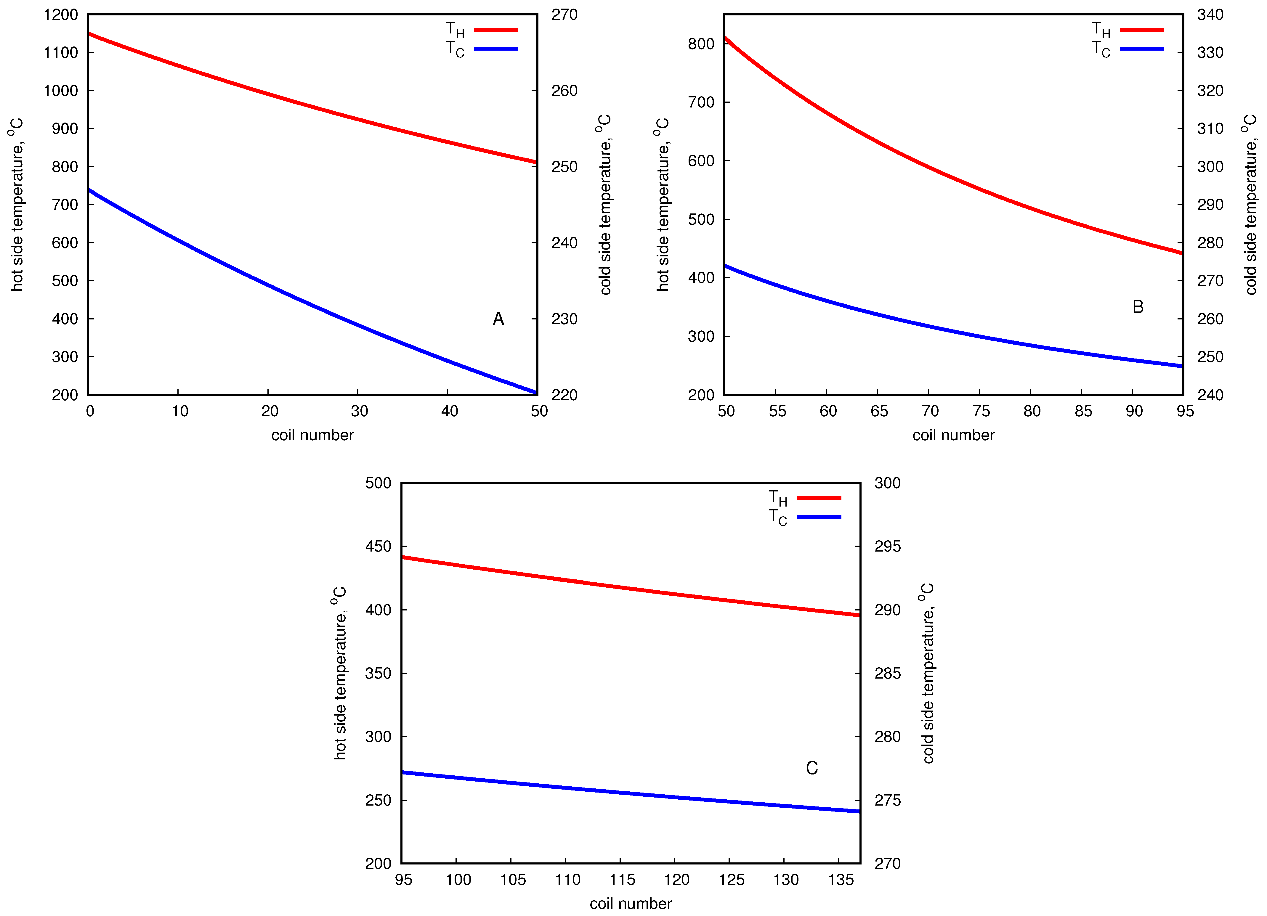
Figure 6 presents the graphs of temperature distribution on the hot and cold sides in A, B and C sections, which are the variation curves typical for the counter-current type of heat exchanger, as assumed in the computations.

3.2. Step II—Four-Pipe HCHE Case

This stage aimed at predicting the thermal performance of a heat exchanger of a similar helically coiled type design but with an additional tube (outer) and a given thermal capacity. Likewise, in this case, four different flow sections within the heat exchanger were taken into consideration, as demonstrated in Figure 7:
  • zone A—flue gas flow in the inner coil core,
  • zone B—covering flue gas annular flow in the volume between the inner and the third coil,
  • zone C—annular flow delineated by the third and fourth coils,
  • zone D—involving flue gas flow between the fourth (outer) coil and the exchanger wall.
The half cross-sectional view of the exchanger with marked flow directions of the hot fluid (flue gas) and the cold fluid (thermal oil) is schematically demonstrated in Figure 7. It is clearly seen that in such a case, the exchanger is considered in terms of a mixed type, i.e., as counter-current in sections A, B and C, and as co-current in section D. Thereby, the determined flue gas temperature at the outlet of the exchanger is averaged between sections A and B.
Thermal and flow parameters, assumed for the calculations are presented in Table 6. The mass flow rate on the cold side (thermal oil) is determined based on the design heat exchanger capacity and outlet/inlet temperature difference of the cooling fluid, whereas the flow rate of exhaust gas is calculated from the general energy balance assuming the thermal oil parameters and the flue gas temperature decrease. The flue gas composition taken was the same as in the case of a 3-pipe HCHE (see Table 4). Similarly, the physical properties of Therminol 66 ([45]) were adopted for calculations.
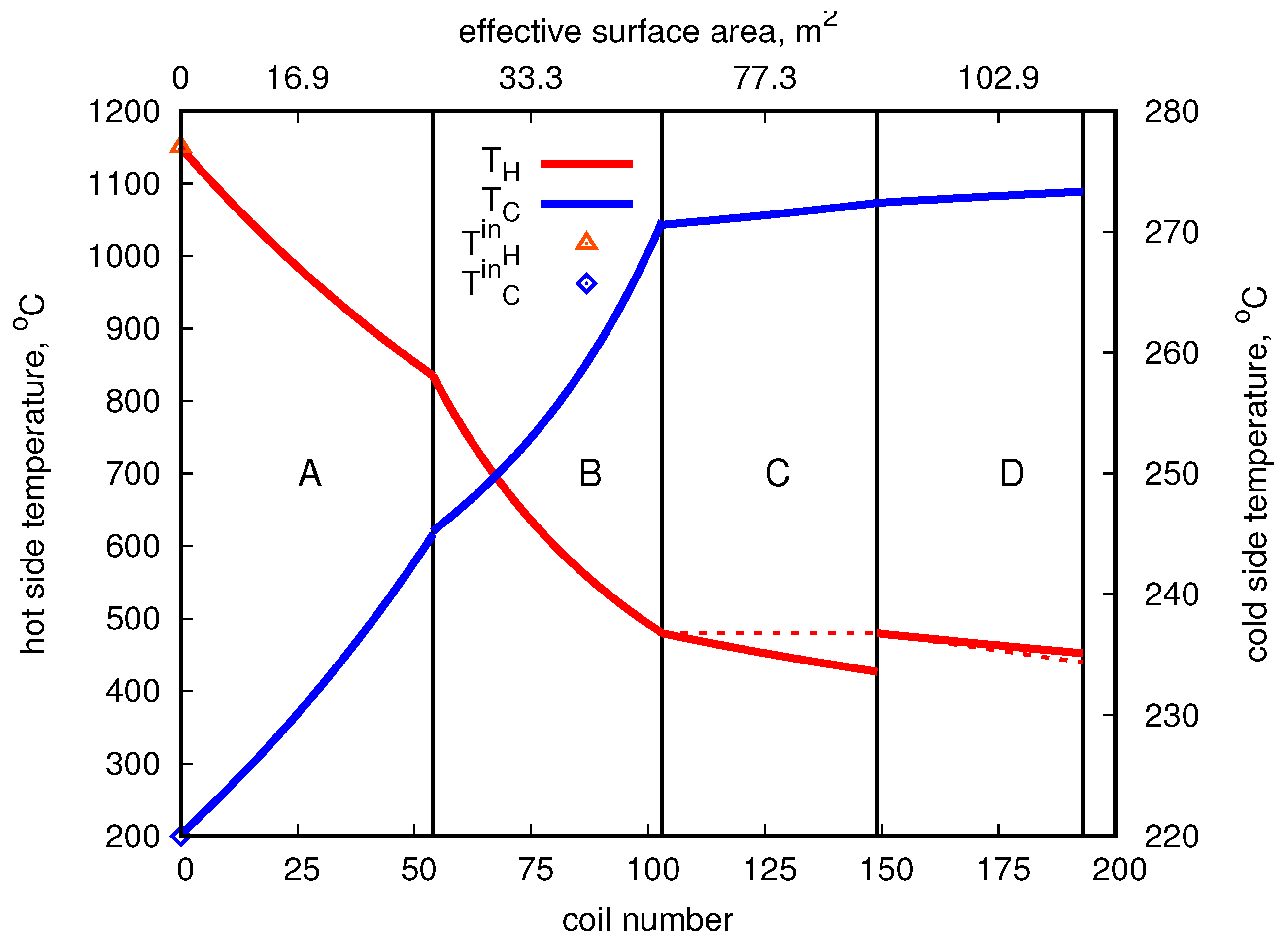
Like in the previous case, the temperature limits were adopted. For oil, it was set not higher than 280 °C, and for flue gas not lower than 350 °C. The flue gas temperature at the inlet into the exchanger was assumed at 1150 °C. The input temperature (points) and the temperature changes of the fluids are shown in Figure 8.
The results reveal that the most intensive heat transfer, as expected, occurs in the first two sections (A and B). One should note that the dashed line in section C in Figure 8 corresponds also with the inlet flue gas temperature in section D, wherein, contrary to sections A–C, the co-current flow is considered (see Figure 7). In addition, owing to the mixed type heat exchanger (counter-current/co-current), at the outlet from the exchanger, the flue gas temperature is taken as an average between the outlet temperatures from sections C and D (Figure 8, dashed line in section D).
The total coil surface area A amounts to 350 m 2 , but the effective heat exchange surface area is over three times lower and it equals to A e f f = 109.36 m 2 . The heat duties of the respective sections are approximately 890 kW, 950 kW, 67 kW and 36 kW, which gives the total capacity of ca. 1945 kW. The detailed data are presented in Table 7.
As seen, the total temperature decrease of the exhaust gases exceeds 710 degrees, which with the analyzed flow and geometrical parameters gives over 50 °C increase in oil temperature.
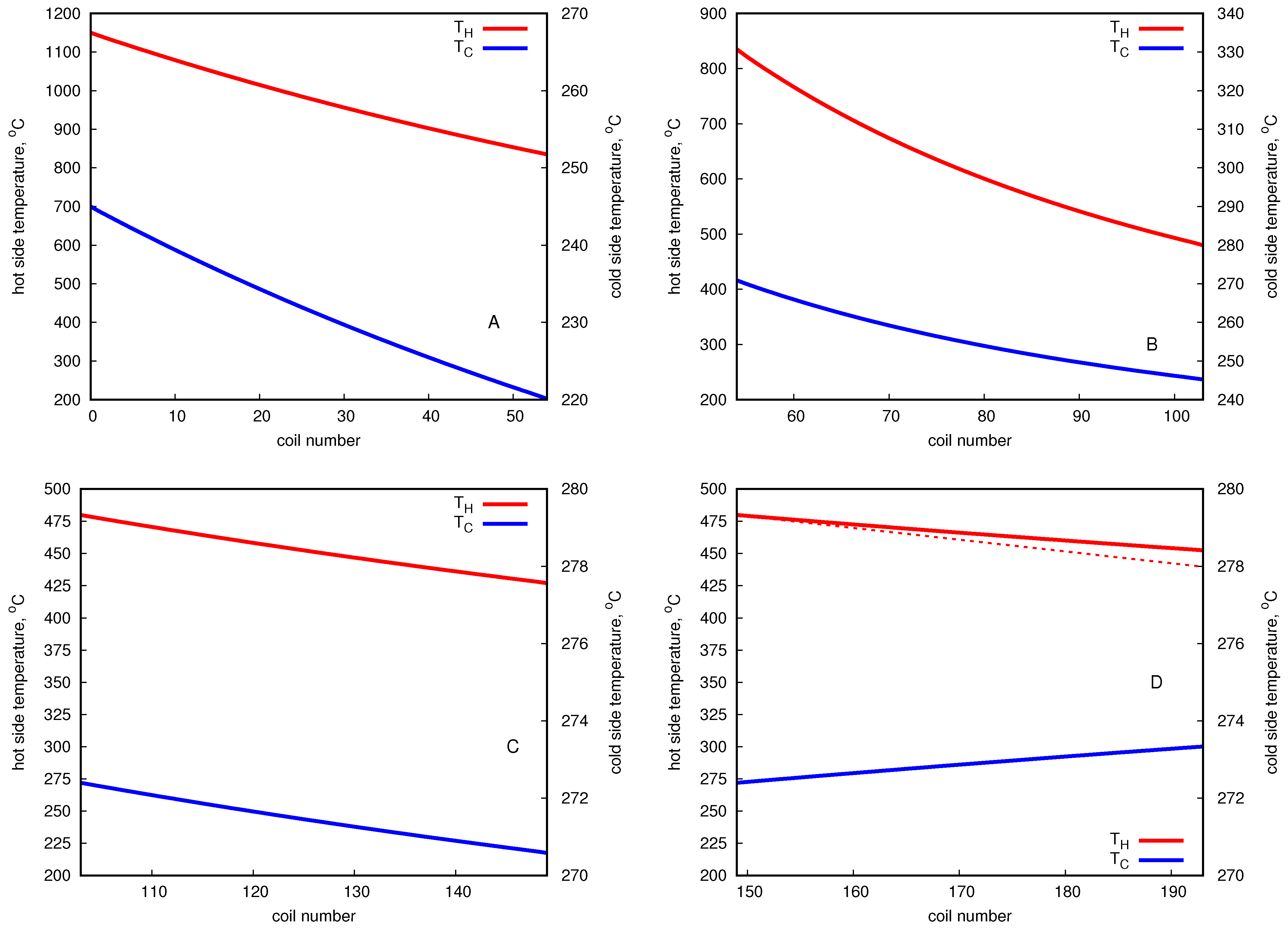
In Figure 9, the graphs for temperature distribution at each section are presented. The first three sections (A, B and C) represent the counter-current type of heat exchanger, and the last one (D) is a co-current type of heat exchanger.
In analyzed cases, the assumption of heating the thermal oil to 280 °C was almost achieved. One should note that another important aspect in the design of exchangers with such a type of coolant must be accounted for. Namely, the protection of the device in case of unexpected significant changes in parameters (e.g., temperature and pressure), beyond the range of operating parameters of both the working fluid (oil) and the installation itself, which may result, for example, in a fire of the installation. It is, therefore, necessary to equip it with an automation system, taking into account different factors. In the case of no or too little oil flow through the heat exchanger, the differential pressure switch on the oil inlet and outlet should be used. The safety valve is widely accepted to prevent excessive pressure increase, while a thermostat prevents the maximum temperature from being exceeded. Moreover, in an open system with an expansion tank, the oil level in the tank should be controlled. In this case, a float sensor may be used to disallow the system leakage.
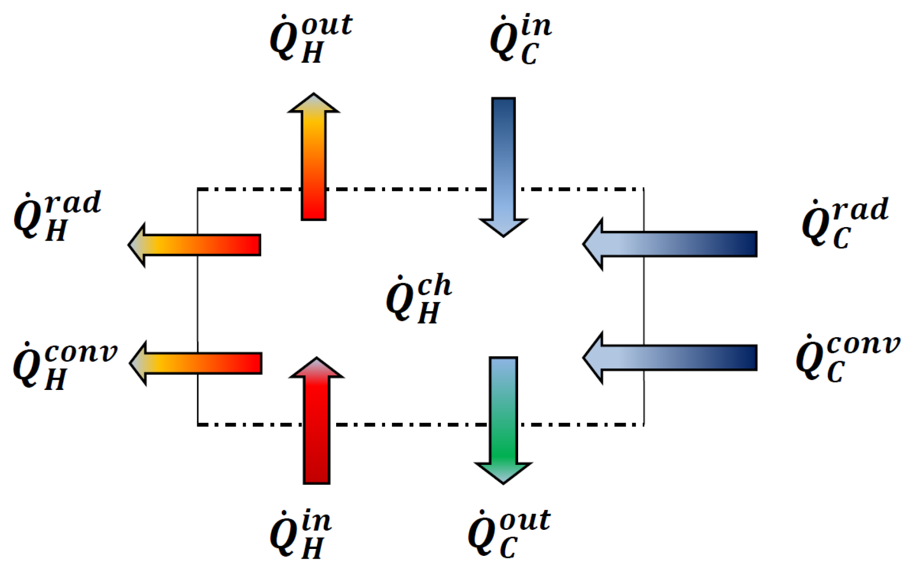
Leaving aside the aforementioned security aspects, it was shown in this paper that the proposed simple and fast mathematical model for determining the thermal and flow performance of helically coiled heat exchangers is a perspective tool for the first step design of heating units. It is a useful tool for geometrically complex systems which are characterized by different types of flow. This approach can be used for analyzing different types of heat exchangers: co-current, counter-current flow, and mixed ones. It is based on a simple stationary energy balance equation between the fluids, taking into account all types of heat transfer (convection, conduction, radiation) whose values depend on the flow parameters and geometry. Moreover, the developed model accounts for temperature-varying physical fluid properties.

4. Conclusions

In this study, the thermal evaluation of helically coiled multi-tube heat exchangers fed with flue gas and cooled with thermal oil was conducted through numerical calculations. To perform the analysis, a one-dimensional multi-section lumped model was developed and implemented in the in-house code.
Two configurations of a concentric helically coiled tube exchanger were analyzed: the three- and four-tube cases. The analysis was conducted in two stages. In the first stage, which covered the calculations for the three-tube case, the developed in-house code was validated with measurement data, showing satisfactory convergence, at about 6% regarding the predicted thermal capacity. In the second stage, the developed methodology was used to determine the thermal performance of a helically coiled tube heat exchanger of larger capacity, other tube dimensions and tube configuration, i.e., four-tube heat exchanger. The thermal power in this case was predicted with an accuracy of less than 12%.
The obtained results demonstrate that the in-house code can serve as an effective design tool when a preliminary heat exchanger geometry is given. It thus comprises an alternative for costly and time-consuming advanced CFD calculations.
Future work should focus on calculating the pressure drop in the system on both sides, the shell side (hot fluid flow) and the tube side (cold fluid flow). This will provide complete information about the thermal and flow characteristics of helically coiled heat exchangers.

Author Contributions

Conceptualization, I.W.-Ś. and S.P.-K., methodology, I.W.-Ś. and S.P.-K.; resources, S.P.-K., I.W.-Ś. and A.D.; writing—original draft preparation, S.P.-K., I.W.-Ś. and A.D.; writing—review and editing, S.P.-K. and I.W.-Ś. All authors have read and agreed to the published version of the manuscript.

Funding

This research received no external funding.

Institutional Review Board Statement

Not applicable.

Data Availability Statement

Data are contained within the article.

Conflicts of Interest

Author Adam Da̧browski was employed by PW “En-Tech” Adam Da̧browski, the remaining authors declare that the research was conducted in the absence of any commercial or financial relationships that could be construed as a potential conflict of interest.

Nomenclature

aabsorptivity
Asurface area, m 2
c p specific heat, J / ( kgK )
dtube diameter, m
Dcoil annulus diameter, m
d h heating value, J / ( kg )
d ϕ coil pitch, m
HHVhigh heating value, J / ( kg )
Lsegment length, m
m ˙ mass flow rate, kg / s
N u Nusselt number
ppressure, Pa
P r Prandtl number
R i n d individual gas constsnt, J / ( kg K )
R e Reynolds number
Q ˙ rate of heat flow, W
Ttemperature, K
vvelocity, m / s
Vvolume, m 3
Greek symbols
α heat transfer coefficient, W / ( m 2 K )
β correction factor
Γ ˙ combustion mass flow rate, kg / s
ϵ emissivity
λ thermal conductivity, W / ( mK )
λ s stoichiometric air-to-fuel mass ratio
ν kinematic viscosity, m 2 / s
μ dynamic viscosity, kg / ( m s )
σ Stefan–Boltzmann constant, 5.67 × 10 8 W / ( m 2 K 4 )
ρ density, kg / m 3
Subscripts/Superscripts
Ccold side
chchemical
convconvection
effeffective
Hhot side
icomputational i-th cell
ininlet
outoutlet
radradiation
tottotal
Abbreviations
CFDComputational Fluid Dynamics
LMTDLogarithmic Mean Temperature Difference
NTUNumber of heat Transfer Units

References

  1. Kim, S.M.; Jo, J.H.; Lee, Y.E.; Yeong-Yoo, S. Comparative Study of Shell and Helically-Coiled Tube Heat Exchangers with Various Dimple Arrangements in Condensers for Odor Control in a Pyrolysis System. Energies 2016, 9, 1027. [Google Scholar] [CrossRef]
  2. Polesek-Karczewska, S.; Turzyński, T.; Kardaś, D.; Heda, L. Front velocity in the combustion of blends of poultry litter with straw. Fuel Process. Technol. 2018, 176, 307–315. [Google Scholar] [CrossRef]
  3. Polesek-Karczewska, S.; Kardaś, D.; Wardach-Święcicka, I. An in-house numerical code to assist in designing a small-scale red-hot air furnace. Arch. Thermodyn. 2023, 44, 43–61. [Google Scholar] [CrossRef]
  4. Lazova, M.; Huisseune, H.; Kaya, A.; Lecompte, S.; Kosmadakis, G.; De Paepe, M. Performance Evaluation of a Helical Coil Heat Exchanger Working under Supercritical Conditions in a Solar Organic Rankine Cycle Installation. Energies 2016, 9, 432. [Google Scholar] [CrossRef]
  5. Yrjoola, Y.; Paavilainen, J. Modelling and analyses of heat exchangers in a biomass boiler plant. Int. J. Energy Res. 2004, 28, 473–494. [Google Scholar] [CrossRef]
  6. Nwokolo, N.; Mukumba, P.; Obileke, K. ThermalPerformanceEvaluation of Double Pipe Heat Exchanger Installed in a Biomass Gasification System. J. Eng. 2020, 6762489. [Google Scholar] [CrossRef]
  7. Majdak, M.; Grądziel, S.; Zima, W.; Cebula, A.; Rerak, M.; Kozak-Jagieła, E. Numerical and experimental analysis of thermal and flow operating conditions of waterwall tubes connected by fins. Arch. Thermodyn. 2023, 44, 81–102. [Google Scholar] [CrossRef]
  8. Omara, M.A.; Abdelatief, M.A. Experimental study of heat transfer and friction factor inside elliptic tube fixed with helical coils. Appl. Therm. Eng. 2018, 134, 407–418. [Google Scholar] [CrossRef]
  9. Sheeba, A.; Abhijith, C.; Jose Prakash, M. Experimental and numerical investigations on the heat transfer and flow characteristics of a helical coil heat exchanger. Int. J. Refrig. 2019, 99, 490–497. [Google Scholar] [CrossRef]
  10. Sigalotti, L.D.G.; Alvarado-Rodríguez, C.E.; Rendón, O. Fluid Flow in Helically Coiled Pipes. Fluids 2023, 8, 308. [Google Scholar] [CrossRef]
  11. Bonafoni, G.; Capata, R. Proposed Design Procedure of a Helical Coil Heat Exchanger for an Orc Energy Recovery System for Vehicular Application. Mech. Mater. Sci. Eng. J. 2015, 1, 72–96. [Google Scholar] [CrossRef]
  12. Nazarova, I.; Gutkowski, A. Experimental investigation of limit parameters of direct contact condensation in the heat exchanger for waste heat recovery. Arch. Thermodyn. 2023, 44, 463–482. [Google Scholar] [CrossRef]
  13. Zarei, A.; Seddighi, S.; Elahi, S.; Orlü, R. Experimental investigation of the heat transfer from the helical coil heat exchanger using bubble injection for cold thermal energy storage system. Appl. Therm. Eng. 2022, 200, 117559. [Google Scholar] [CrossRef]
  14. Hossain, M.A.; Onaka, Y.; Afroz, H.M.; Miyara, A. Heat transfer during evaporation of R1234ze(E), R32, R410A and a mixture of R1234ze(E) and R32 inside a horizontal smooth tube. Appl. Therm. Eng. 2013, 36, 465–477. [Google Scholar] [CrossRef]
  15. Solanki, A.K.; Kumar, R. Condensation of R-134a inside micro-fin helical coiled tube-in-shell type heat exchanger. Exp. Therm. Fluid Sci. 2018, 93, 344–355. [Google Scholar] [CrossRef]
  16. Romaniak, A.; Kowalczyk, M.J.; Łęcki, M.; Gutkowsk, A.; Górecki, G. Investigation of thermal-flow characteristics of the minichannel heat exchanger of variable louvers height. Arch. Thermodyn. 2023, 44, 119–141. [Google Scholar] [CrossRef]
  17. Izadpanah, E.; Zarei, A.; Akhavan, S.; Rabiee, M.B. An experimental investigation of natural convection heat transfer from a helically coiled heat exchanger. Int. J. Refrig. 2018, 93, 38–46. [Google Scholar] [CrossRef]
  18. Taler, D. Engineering Methods for Thermal Calculations of Heat Exchangers. In Studies in Systems, Decision and Control; Springer: Cham, Switzerland, 2019; pp. 303–320. [Google Scholar] [CrossRef]
  19. Borjigin, S.; Zhang, S.; Zeng, M.; Wang, Q.; Ma, T. Coupling ϵ-NTU method for thermal design of heat exchanger in cabinet cooling system. Appl. Therm. Eng. 2019, 159, 113972. [Google Scholar] [CrossRef]
  20. Li, H.; Huang, H.; Xu, G.; Wen, J.; Wu, H. Performance analysis of a novel compact air-air heat exchanger for aircraft gas turbine engine using LMTD method. Appl. Therm. Eng. 2017, 116, 445–455. [Google Scholar] [CrossRef]
  21. Tuncer, A.D.; Sozen, A.; Khanlari, A.; Gürbüz, E.Y.; Variyenli, H.I. Analysis of thermal performance of an improved shell and helically coiled heat exchanger. Appl. Therm. Eng. 2021, 184, 116272. [Google Scholar] [CrossRef]
  22. Omidia, M.; Farhadia, M.; Darzi, A.A.R. Numerical study of heat transfer on using lobed cross sections in helical coil heat exchangers: Effect of physical and geometrical parameters. Energy Convers. Manag. 2018, 176, 236–245. [Google Scholar] [CrossRef]
  23. Abu-Hamdeh, N.H.; Bantan, R.A.; Tlili, I. Analysis of the thermal and hydraulic performance of the sector-by-sector helically coiled tube heat exchangers as a new type of heat exchangers. Int. J. Therm. Sci. 2020, 150, 106229. [Google Scholar] [CrossRef]
  24. Abu-Hamdeh, N.H.; Alsulami, R.A.; Rawa, M.J.; Aljinaidi, A.A.; Alazwari, M.A.; Eltaher, M.A.; Almitani, K.H.; Alnefaie, K.A.; Abusorrah, A.M.; Sindi, H.F.; et al. A detailed hydrothermal investigation of a helical micro double-tube heat exchanger for a wide range of helix pitch length. Case Stud. Therm. Eng. 2021, 28, 101413. [Google Scholar] [CrossRef]
  25. Elsaid, A.M.; Ammar, M.; Lashin, A.; Assassa, G.M. Performance characteristics of shell and helically coiled tube heat exchanger under different tube cross-sections, inclination angles and nanofluids. Case Stud. Therm. Eng. 2023, 49, 103239. [Google Scholar] [CrossRef]
  26. Kurnia, J.C.; Sasmito, A.P.; Shamim, T.; Mujumdar, A.S. Numerical investigation of heat transfer and entropy generation of laminar flow in helical tubes with various cross sections. Appl. Therm. Eng. 2016, 102, 849–860. [Google Scholar] [CrossRef]
  27. Haskins, D.; El-Genk, M. CFD analyses and correlation of pressure losses on the shell-side of concentric, helically-coiled tubes heat exchangers. Nucl. Eng. Des. 2016, 305, 531–546. [Google Scholar] [CrossRef]
  28. Kardaś, D.; Wardach-Święcicka, I.; Grajewski, A. Partially transient one-dimensional thermal-flow model of a heat exchanger, upwind numerical solution method and experimental verification. Arch. Thermodyn. 2022, 43, 63–83. [Google Scholar] [CrossRef]
  29. Sogni, A.; Chiesa, P. Calculation code for helically coiled heat recovery boilers. Energy Procedia 2014, 45, 492–501. [Google Scholar] [CrossRef]
  30. Andrzejczyk, R.; Muszyński, T. Performance analyses of helical coil heat exchangers. The effect of external coil surface modification on heat exchanger effectiveness. Arch. Thermodyn. 2016, 37, 137–159. [Google Scholar] [CrossRef]
  31. Alimoradi, A. Study of thermal effectiveness and its relation with NTU in shell and helically coiled tube heat exchangers. Case Stud. Therm. Eng. 2017, 9, 100–107. [Google Scholar] [CrossRef]
  32. Panahi, D.; Zamzamian, K. Heat transfer enhancement of shell-and-coiled tube heat exchanger utilizing helical wire turbulator. Appl. Therm. Eng. 2017, 115, 607–615. [Google Scholar] [CrossRef]
  33. Mirgolbabaei, H. Numerical investigation of vertical helically coiled tube heat exchangers thermal performance. Appl. Therm. Eng. 2018, 136, 252–259. [Google Scholar] [CrossRef]
  34. Polesek-Karczewska, S.; Wardach-Święcicka, I.; Kardaś, D.; Turzyński, T. Application of a Lumped Multi-Section Model for Analyzing the Thermal Performance of a Small-Scale Biomass Boiler. J. Therm. Sci. 2021, 30, 1034–1045. [Google Scholar] [CrossRef]
  35. Boilers with thermal oil EN-0D type-En-tech Materials. Available online: http://www.en-tech.pl/download/ENOD_File2.pdf (accessed on 1 November 2024).
  36. En-tech Investments. Available online: http://www.en-tech.pl/inwestycjeang.htm (accessed on 1 November 2024).
  37. Press, W.; Teukolsky, S.; Vetterling, W.; Flannery, B. Numerical Recipes in Fortran 90, the Art of Parallel Scientific Computing, Volume 2 of Fortran Numerical Recipes, 2nd ed.; Cambridge University Press: Cambridge, UK, 1997. [Google Scholar]
  38. Jayakumar, J. Helically Coiled Heat Exchangers, Heat Exchangers—Basics Design Applications; Mitrovic, J., Ed.; InTechOpen: Rijeka, Croatia, 2012; ISBN 978-953-51-0278-6. [Google Scholar]
  39. Naphon, P.; Wongwises, S. A review of flow and heat transfer characteristics in curved tubes. Renew. Sustain. Energy Rev. 2006, 10, 463–490. [Google Scholar] [CrossRef]
  40. Klein, M.; Heda, Ł.; Kluska, J.; Kazimierski, P. Physicochemical Analysis of Wood Pellets; Unpublished Technical Report; IFFM PAS: Gdańsk, Poland, 2013. [Google Scholar]
  41. Kardaś, D.; Turzyński, T.; Wardach-Święcicka, I.; Ronewicz, K. Combustion and Heat Exchange in Biomass-Based Oil Boiler; IFFM Publishers: Gdańsk, Poland, 2014; ISBN 978-83-88237-33-1. (In Polish) [Google Scholar]
  42. Simanjuntak, J.P.; Daryanto, E.; Tambunan, B. An operating parameter study of the biomass solid feedstock incinerator of fixed-bed type with two stage air supply. J. Phys. Conf. Ser. 2022, 2193, 012077. [Google Scholar] [CrossRef]
  43. McBride, B.; Zehe, M.; Gordon, S. NASA Glenn Coefficients for Calculating Thermodynamic Properties of Individual Species; Tech Rep TP-2002-211556; NASA: Hanover, MA, USA, 2002. [Google Scholar]
  44. Air—Dynamic and Kinematic Viscosity. Available online: https://www.engineeringtoolbox.com/air-absolute-kinematic-viscosity-d_601.html (accessed on 1 November 2024).
  45. Therminol 66. High Performance, Highly Stable Heat Transfer Fluid. Available online: https://www.therminol.com/product/71093438?pn=Therminol-66-Heat-Transfer-Fluid (accessed on 2 February 2024).
  46. Shell Thermia Oil B—High Performance Heat Transfer Fluid. Available online: https://lubricanthub.com/shell-thermia-oil-high-performance-heat-transfer-fluid/ (accessed on 1 November 2024).
  47. Lienhard IV, J.; Lienhard V, J. A Heat Transfer Textbook, 6th ed.; Phlogiston Press: Cambridge, MA, USA, 2024. [Google Scholar]
  48. Serth, R.; Lestina, T. Process Heat Transfer, Principles, Applications and Rules of Thumb; Elsevier: Amsterdam, The Netherlands, 2007. [Google Scholar]
Figure 1. Scheme and the real view of the thermal-oil heating unit (En-tech).
Sustainability 17 00759 g001
Figure 2. Heat fluxes in i-th cell—diagram for the case of counter-current flow in the one-dimensional lumped multi-section model.
Sustainability 17 00759 g002
Figure 3. 3D cross-sectional view of the helical coil cutout with main dimensions marked.
Sustainability 17 00759 g003
Figure 4. Diagram of the half cross-section of the 3-pipe heat exchanger (from axis to the wall) with the flow directions of fluids marked.
Sustainability 17 00759 g004
Figure 5. The predicted temperature changes of fluids for case I; A, B, C—heat exchanger sections.
Sustainability 17 00759 g005
Figure 6. The predicted temperature changes of fluids in each heat exchanger section: A (top left), B (top right), and C (bottom)—case I.
Sustainability 17 00759 g006
Figure 7. Diagram of the half cross-section of the 4-pipe heat exchanger (from axis to the wall) with the flow directions of fluids marked.
Sustainability 17 00759 g007
Figure 8. The predicted temperature changes of fluids—case II; A, B, C, D—heat exchanger sections.
Sustainability 17 00759 g008
Figure 9. The predicted temperature changes of fluids in each heat exchanger section: A (top left), B (top right), C (bottom left), and D (bottom right)—case II.
Sustainability 17 00759 g009
Table 1. Particular terms of the proposed mathematical model’s governing Equations (2) and (4).
Hot SideCold Side
Q ˙ H , i i n = m ˙ H i n c p , H T H , i T H i n (2a) Q ˙ C , i i n = m ˙ C i n c p , C T C , i T C i n (4a)
Q ˙ H , i o u t = m ˙ H o u t c p , H T H , i T H o u t (2b) Q ˙ C , i o u t = m ˙ C o u t c p , C T C , i T C o u t (4b)
Q ˙ H c h i = Γ ˙ i d h i (2c)
Q ˙ H r a d i = A ϵ w a l l σ ε H , i T H , i 4 a H , i T w a l l , i 4 (2d) Q ˙ C r a d i = A ϵ w a l l σ T w a l l , i 4 T C , i 4 (4c)
Q ˙ H c o n v i = α H , i A T H , i T w a l l , i (2e) Q ˙ C c o n v i = α C , i A T w a l l , i T C , i (4d)
Table 2. Ultimate and proximate analyses of the organic type fuel adopted for simulation.
Ultimate Analysis, wt%dbProximate Analysis, wt%
C48.50Volatile matter71.55
H5.30Fixed carbon20.28
O45.78Moisture6.10
N0.42Ash2.07
HHV, (MJ/kg)18.28
Table 3. Coefficients for correlation (10), based on data [43].
Coefficient H 2 O CO 2 O 2 N 2
T  < 1000 K
a j × 10 5 J K / mol −7.724.112.851.84
b j × 10 3 J / ( mol ) 13.01−5.214.03−3.18
c j × 10 1 J / ( mol K ) −4.974.4193.045.06
d j × 10 2 J / ( mol K 2 ) 27.192.083.57−7.09
e j × 10 6 J / ( mol K 3 ) −326.94−1.775.68115.13
f j × 10 9 J / ( mol K 4 ) 208.63−6.39−16.82−80.03
g j × 10 12 J / ( mol K 5 ) 53.752.378.6420.95
T  > 1000 K
a j × 10 5 J K / mol 123.849.79−86.3048.87
b j × 10 4 J / ( mol ) −4.30−1.491.95−1.86
c j × 10 1 J / ( mol K ) 9.386.901.515.04
d j × 10 4 J / ( mol K 2 ) 6.69−7.67105.42−51.05
e j × 10 8 J / ( mol K 3 ) 15.124.04−181.93124.04
f j × 10 11 J / ( mol K 4 ) 5.78−1.5717.08−15.99
g j × 10 15 J / ( mol K 5 ) 4.015.26−6.818.83
Table 4. Input calculation data—case I.
Geometrical ParameterFlow Parameter
D b m2.83 m ˙ H kg / s 1.21 *
Lm4.70 T H i n °C1150.0 *
D A m1.695 T H o u t °C 350.0
D B m2.070 m ˙ C kg / s 8.31 *
D C m2.510 T C i n °C220.0
dm0.0809 T C o u t °C280.0
d φ m0.0809 Q ˙ kW 1187.67
N A 50Flue gas composition
N B 45 H 2 O %9.0
N C 42 CO 2 %13.0
A t o t m 2 226.02 O 2 %8.0
N 2 %70.0
* input parameters for verification calculations.
Table 5. Output calculation data—case I.
SectionABCTotal
SideHotColdHotColdHotColdHotCold
m ˙ kg / s 1.218.311.218.311.218.311.218.31
T i n °C1150.00220.22810.67247.28441.31273.841150.00220.22
T o u t °C810.67247.00441.31273.8395.52276.95395.52276.95
Δ T °C339.3326.78369.3626.5245.793.11754.4856.73
Q ˙ kW 516.50516.50533.73533.7364.0164.011114.211114.21
A m 2 33.87150.0442.11225.95
A e f f m 2 10.5946.8813.1670.63
error% 6.18
Table 6. Input calculation data—case II.
Geometrical ParameterFlow Parameter
D b m3.21 m ˙ H kg / s 2.24
Lm5.06 T H i n °C 1150.0
D A m1.695 T H o u t °C 350.0
D B m2.070 m ˙ C kg / s 15.39
D C m2.510 T C i n °C220.0
D D m2.89 T C o u t °C280.0
dm0.0809 Q ˙ kW 2200.0
d φ m0.0809
N A 54Flue gas composition
N B 49 H 2 O %9.0
N C 46 CO 2 %13.0
N C 44 O 2 %8.0
A t o t m 2 349.95 N 2 %70.0
Table 7. Input calculation data—case II.
SectionABCDTotal
SideHotColdHotColdHotColdHotColdHotCold
m ˙ kg / s 2.2415.392.2415.392.2415.392.2415.392.2415.39
T i n °C1150.00220.13834.89245.23479.73273.84479.73272.401150.00220.13
T o u t °C834.89245.00479.73270.90426.80276.95452.33273.34439.56273.34
Δ T °C315.1124.87355.1625.6752.933.1127.40.94710.4453.21
Q ˙ kW 886.79886.79953.24953.2468.868.835.735.71944.531944.53
A m 2 36.58163.3799.2250.78349.95
A e f f m 2 11.4351.0631.0015.87109.36
error% 11.6
Disclaimer/Publisher’s Note: The statements, opinions and data contained in all publications are solely those of the individual author(s) and contributor(s) and not of MDPI and/or the editor(s). MDPI and/or the editor(s) disclaim responsibility for any injury to people or property resulting from any ideas, methods, instructions or products referred to in the content.

