
Modeling and Numerical Analysis of the Severobaikalsk Section of the Baikal–Amur Mainline Considering Environmental Points


Abstract
1. Introduction
2. Literature Review
3. Object of Study
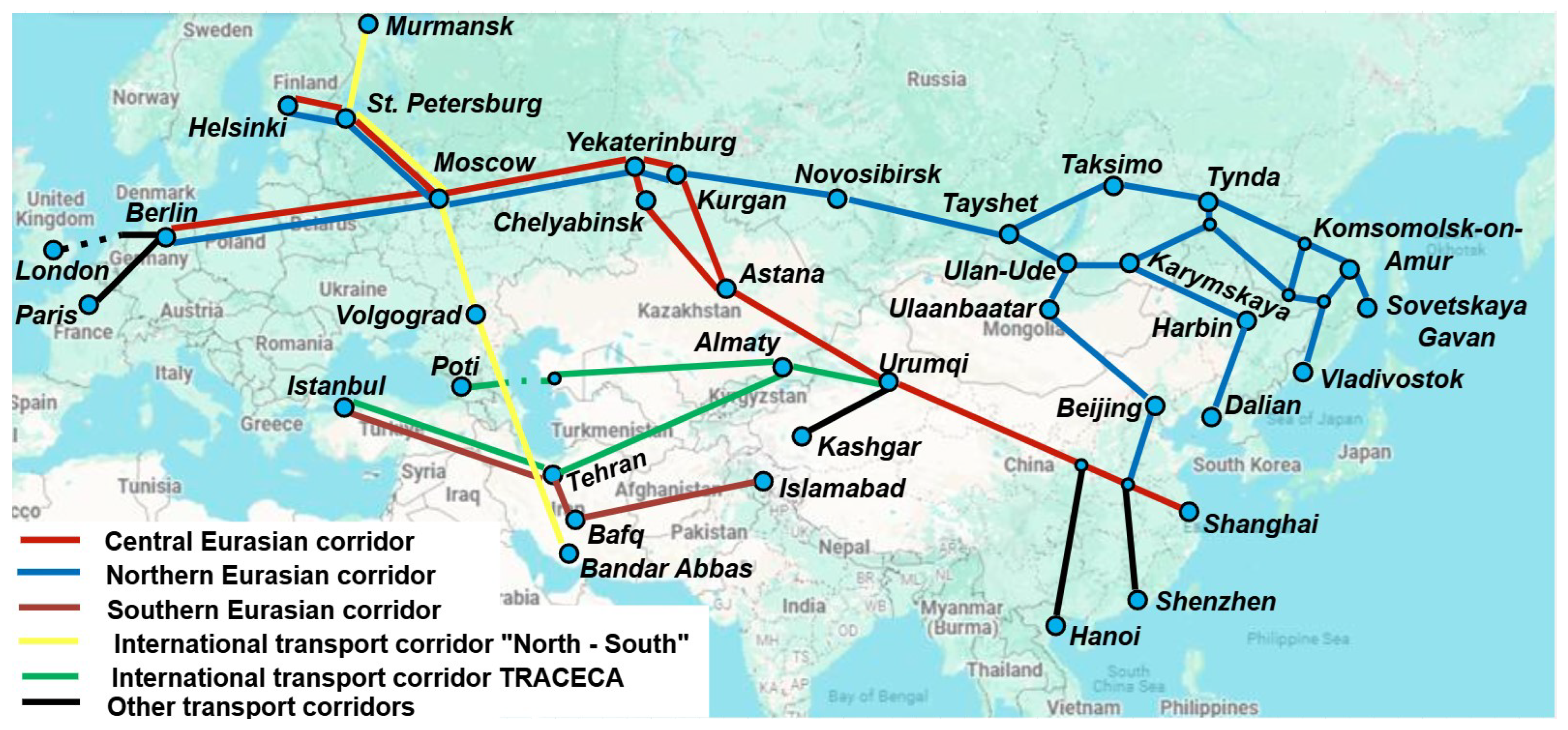
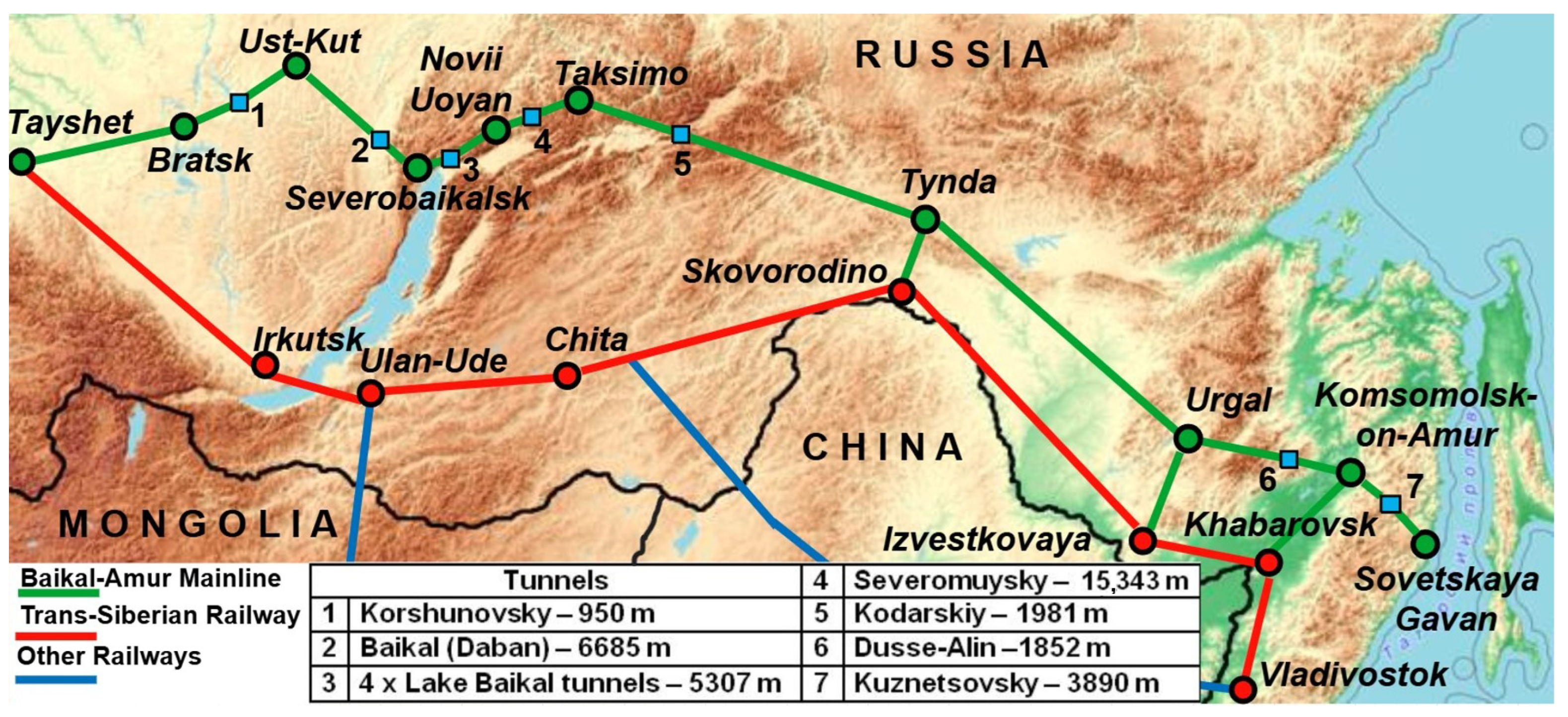
3.1. General Characteristics of Baikal–Amur Mainline
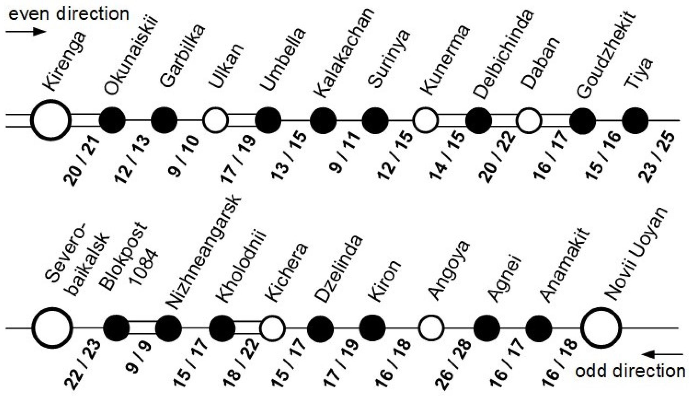
3.2. Severobaikalsk Section of the Baikal–Amur Mainline
4. Methodology of Modeling of Train Traffic in a Railway Section
4.1. Key Features of the Railway Section
4.2. The Methodology and Mathematical Apparatus
- is the probability that a request serviced at node y will go to node u;
- is the probability that a request arrives from the source at node u, ;
- is the probability that a request will leave the SOQN immediately after completion of service in node y.
5. Structural and Parametric Identification of the Model
5.1. Characteristic of Severobaikalsk Section
5.2. Mathematical Model
5.2.1. Incoming Train Flows
- 1.
- Passenger and transit freight trains running in the eastern direction;
- 2.
- Passenger and transit freight trains running in the western direction;
- 3.
- Local freight trains heading east;
- 4.
- Local freight trains heading west.
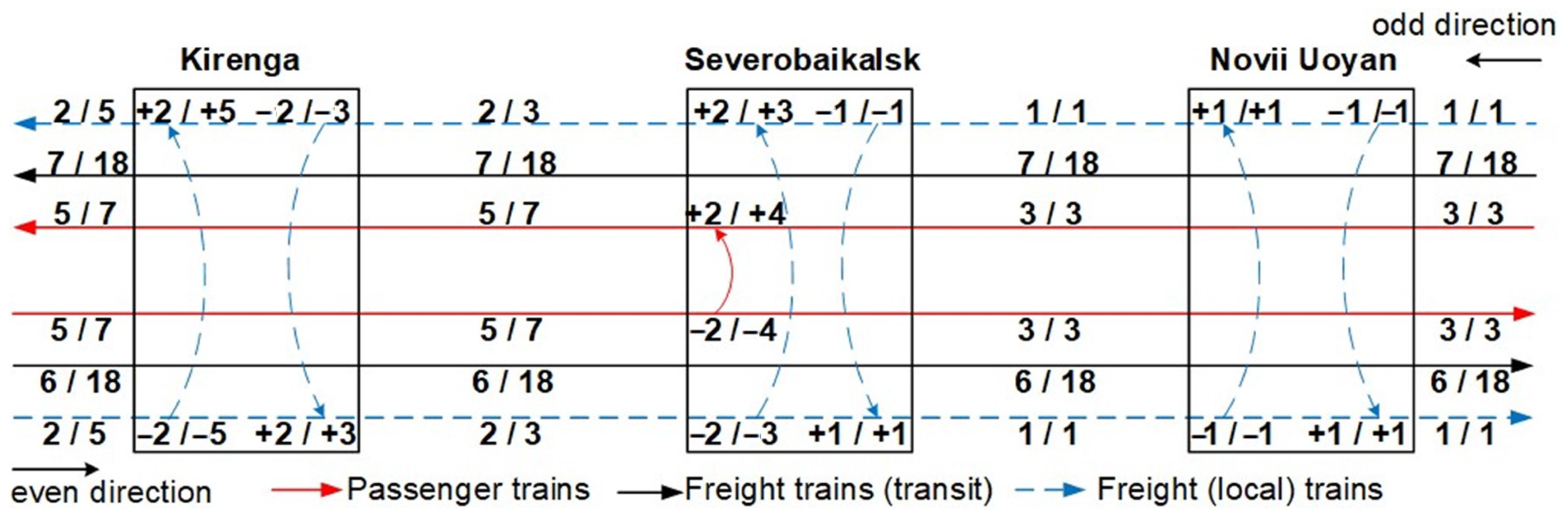
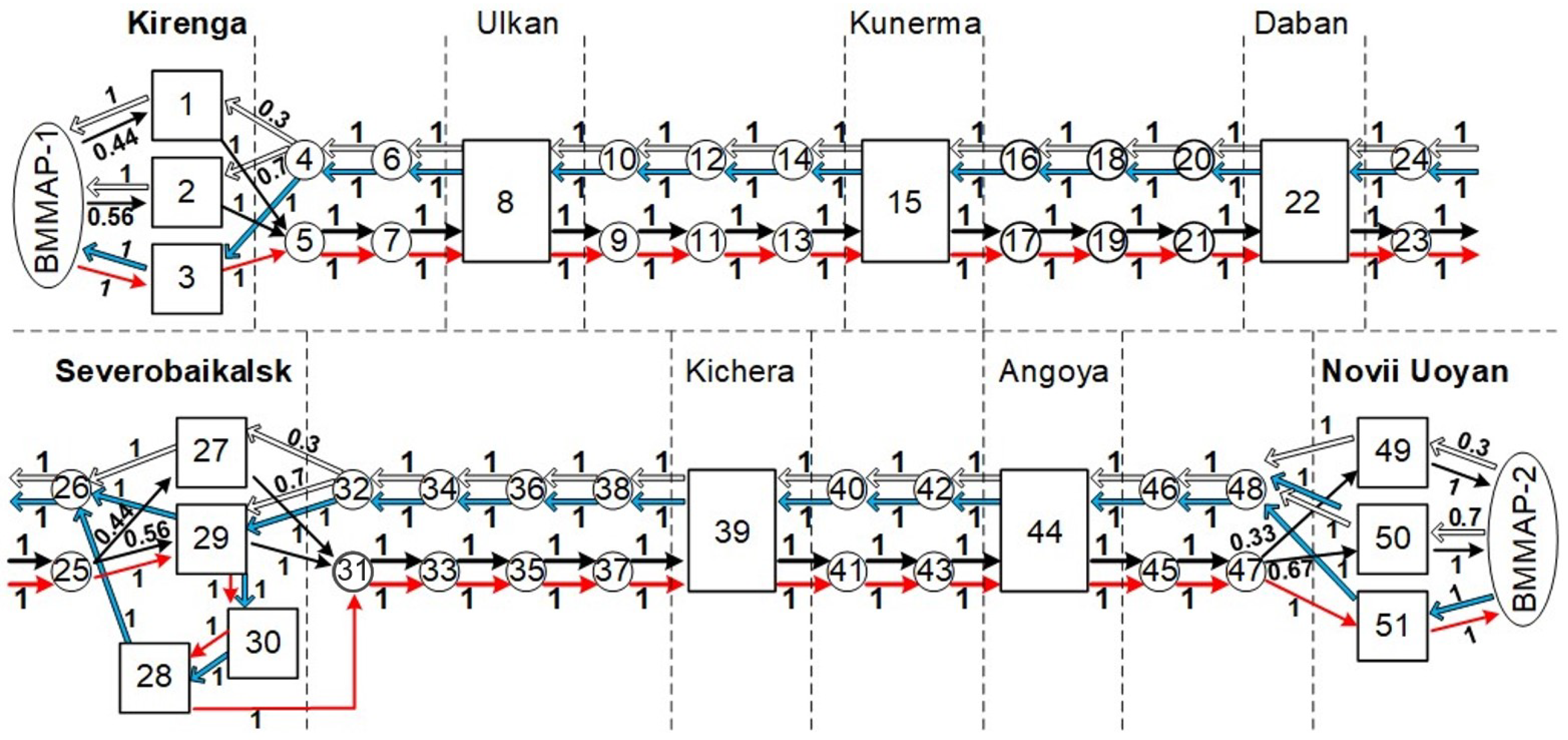
5.2.2. Structural Elements
5.2.3. Train Routes
6. Numerical Experiments
- The first experiment aims to check the adequacy of the constructed model and assess the current load of the section under consideration based on field observation.
- The second experiment addresses determining bottlenecks in system structure and evaluating its maximum capacity.
- The third analyzes the throughput capacity of the Severobaikalsk section when eliminating the identified bottlenecks.
- The fourth studies an alternative method for increasing the capacity of the railway section by using a partial batch train schedule.
- V is the total number of requests arrived at the system in 60 days;
- is the loss probability;
- and are average sojourn time of a request in the SOQN, which describe the running of passenger and transit freight trains in one direction, respectively;
- is an average total time (in minutes) of blocking one request when passing all nodes in one direction, i.e., the total waiting time for departure for an individual passenger or transit freight train on the entire section;
- is a number of requests arrived at node y during the simulation;
- is a channel occupancy rate at node y;
- is an average queue length at node y;
- is an average sojourn time of a request at node y;
- is an average time (in minutes) for one request to stay in a blocked channel at node y (hereinafter referred to as the average blocking time).
6.1. Experiment 1
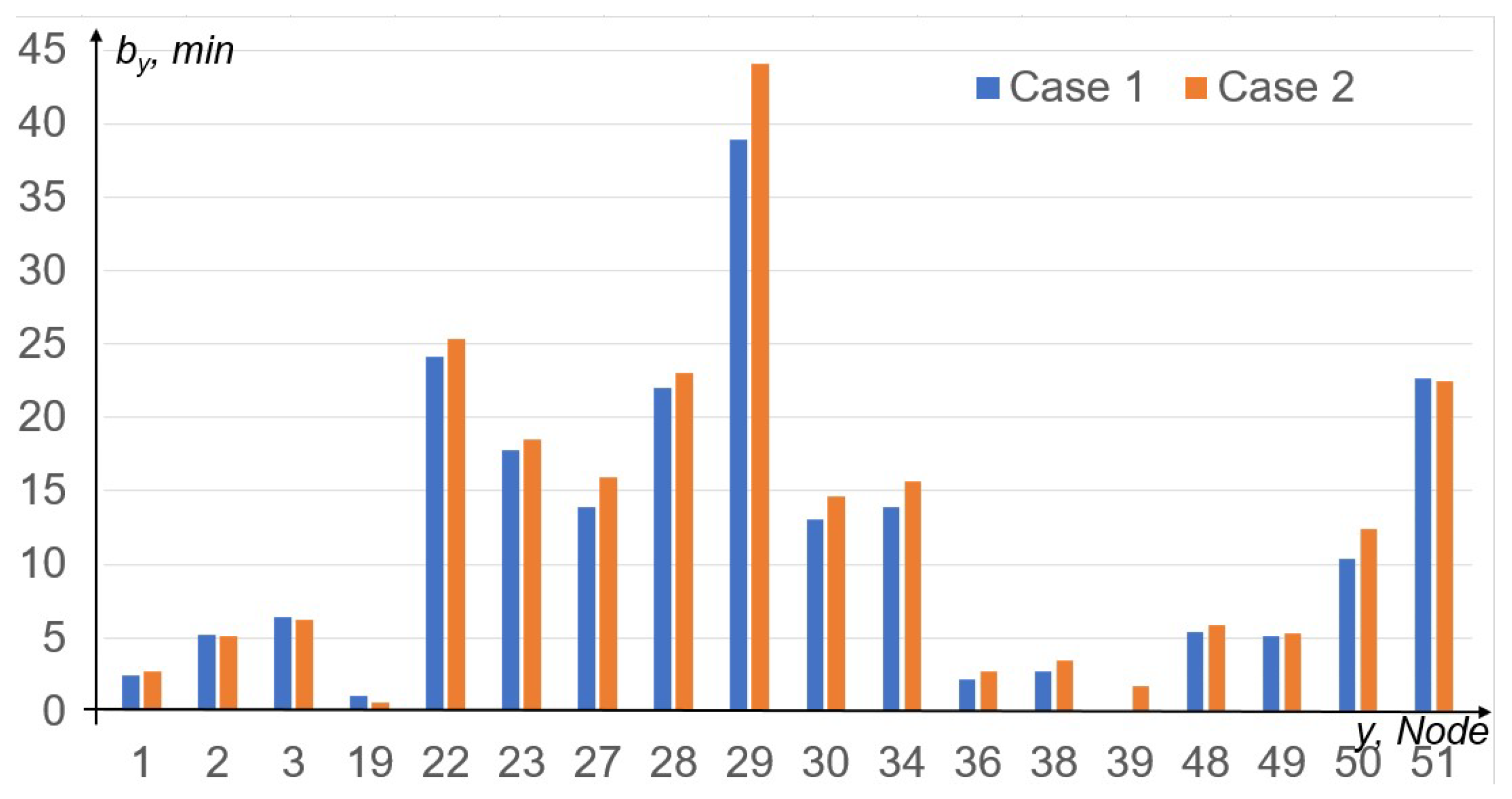
6.2. Experiment 2
- 1.
- The BMMAP1 matrices describing the arrival of 30 trains from the west arewhile the BMMAP2 matrices corresponding to the arrival of 22 trains from the east are
- 2.
- Initially, at Node 22, there is one request of type 3 and one request of type 4. Thus, the number of circulating requests between Nodes 3 and 30 increases to six, corresponding to the number of local freight trains running between Kirenga and Severobaikalsk.
- 3.
- The probabilities of arrival of type 1 requests at Nodes 1, 2, 27, 29, 49 and 50 are , , , , and those of type 2 requests are , , , , respectively. These changes are necessary to reflect the new ratio of passenger and transit freight trains.
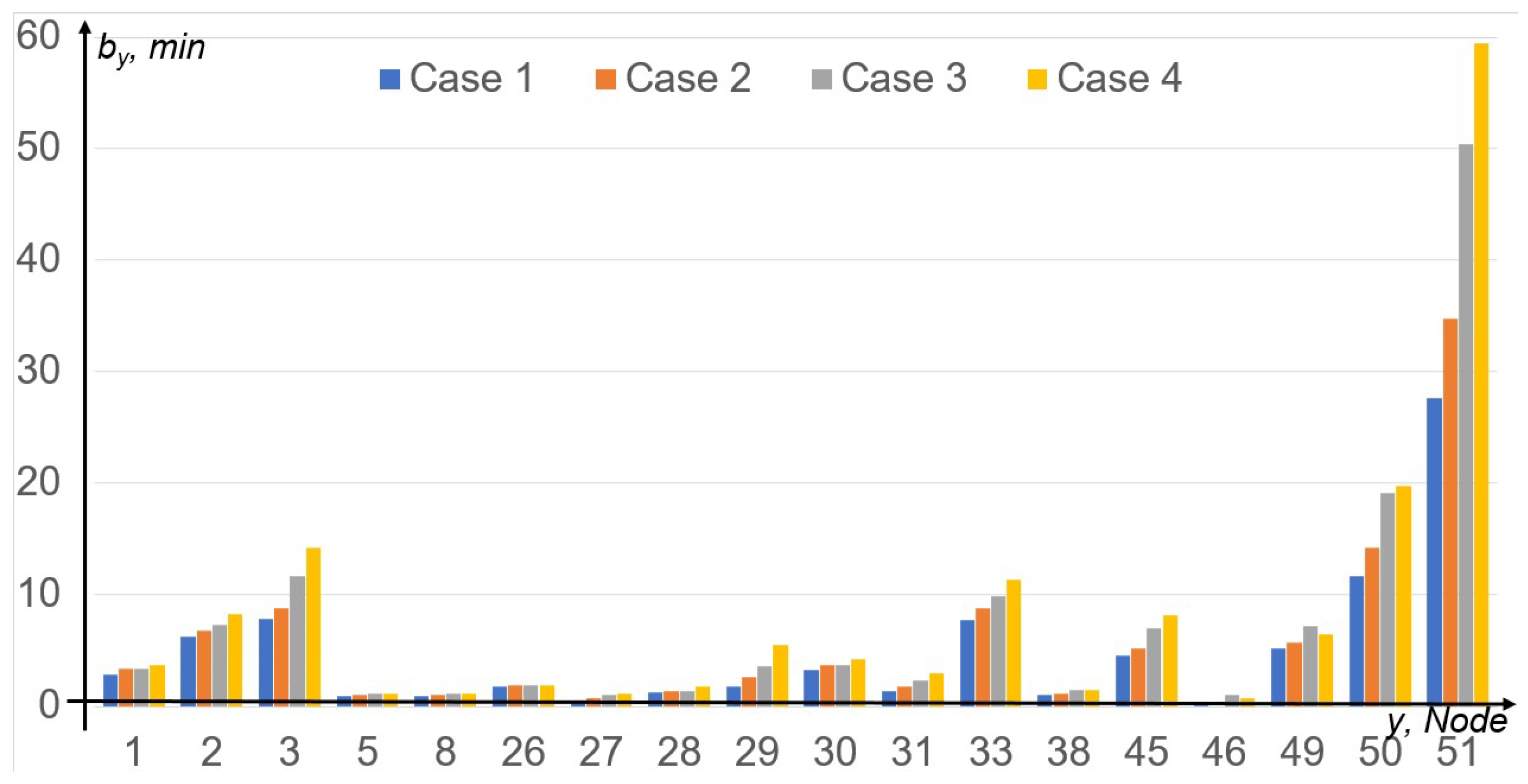
6.3. Experiment 3
- 1.
- Nodes 25, 26, 45, and 46 model the original Goudzhekit–Severobaikalsk and Angoya–Agnei sections, which, recall, consist of two lines and one siding. With double-track traffic, up to three trains can simultaneously run in the same direction, so the number of channels in Nodes 25, 26, 45, and 46 should be increased to three.
- 2.
- Nodes 31 and 32 describe the train running along the Severobaikalsk–Blokpost without a siding. With double-track traffic, the travel time along it in each direction is, on average, 22 min. Then, the service time at Nodes 31 and 32 is reduced by half and obeys .
- 3.
6.4. Experiment 4
6.5. Overall Numerical Results
7. Discussion
8. Conclusions
Author Contributions
Funding
Institutional Review Board Statement
Informed Consent Statement
Data Availability Statement
Conflicts of Interest
Abbreviations
| BAM | Baikal–Amur Mainline |
| BMMAP | Batch Marked Markovian Arrival Process |
| SOQN | Semi-open queuing network |
| QN | Queuing network |
| QS | Queuing system |
References
- Fonseca-Soares, D.A.; Eliziario, S.A.; Galvincio, J.D.; Ramos-Ridao, A.F. Greenhouse Gas Emissions in Railways: Systematic Review of Research Progress. Buildings 2024, 14, 539. [Google Scholar] [CrossRef]
- Tostes, B.; Henriques, S.T.; Brockway, P.E.; Heun, M.K.; Domingos, T.; Sousa, T. On the right track? Energy use, carbon emissions, and intensities of world rail transportation, 1840–2020. Appl. Energy 2024, 367, 123344. [Google Scholar] [CrossRef]
- World Energy Outlook 2023. Available online: https://www.iea.org/reports/world-energy-outlook-2023 (accessed on 7 November 2024).
- Vinokurov, E.; Amangeldy, S.; Ahunbaev, A.; Zaboev, A.; Kuznetsov, A.; Malakhov, A. The Eurasian Transport Network, Reports 24/6; Eurasian Development Bank: Almaty, Kazakhstan, 2024; 142p. [Google Scholar]
- Order of the Government of the Russian Federation dated 04/28/2021 N 1100-p: On Approval of the Passport of the Investment Project “Modernization of the Railway Infrastructure of the Baikal-Amur and Trans-Siberian Railway with the Development of Capacity and Carrying Capacity (Second Stage)” [Rasporyazhenie Pravitel’stva RF ot 28.04.2021 № 1100-r: Ob Utverzhdenii Pasporta Investicionnogo Proekta «Modernizaciya Zheleznodorozhnoj Infrastruktury Bajkalo-Amurskoj i Transsibirskoj Zheleznodorozhnyh Magistralej s Razvitiem Propusknyh i Provoznyh Sposobnostej (Vtoroj Etap)»]. Available online: https://base.garant.ru/400726399/ (accessed on 7 November 2024). (In Russian).
- Shcherbanin, Y.A. Transport in Russia: Nine Years of Economic Sanctions. Stud. Russ. Econ. Dev. 2023, 34, 592–600. [Google Scholar] [CrossRef]
- Kazakov, A.; Lempert, A.; Zharkov, M. Modeling a Section of a Single-Track Railway Network Based on Queuing Networks. In Information Technologies and Mathematical Modelling. Queueing Theory and Applications; Dudin, A., Nazarov, A., Moiseev, A., Eds.; ITMM 2022. CCIS, 1803; Springer: Cham, Switzerland, 2023. [Google Scholar] [CrossRef]
- Kazakov, A.; Lempert, A.; Zharkov, M. An approach to railway network sections modeling based on queuing networks. J. Rail Transp. Plan. Manag. 2023, 27, 100404. [Google Scholar] [CrossRef]
- Bolch, G.; Greiner, S.; de Meer, H.; Trivedi, K.S. Queueing Networks and Markov Chains: Modeling and Performance Evaluation with Computer Science Applications; John Wiley & Sons, Inc.: New York, NY, USA, 2006; 878p. [Google Scholar] [CrossRef]
- Dudin, A.; Klimenok, V.; Vishnevsky, V. The Theory of Queuing Systems with Correlated Flows; Springer Nature: Cham, Switzerland, 2019; 431p. [Google Scholar] [CrossRef]
- Pyrgidis, C.N. Railway Transportation Systems. Design, Construction and Operation; CRC Press: Boca Raton, FL, USA, 2016; 500p. [Google Scholar] [CrossRef]
- Milenkovic, M.; Bojovic, N. Optimization Models for Rail Car Fleet Management; Elsevier Inc.: Amsterdam, The Netherlands, 2019; 282p. [Google Scholar]
- Sun, Y.; Cao, C.; Wu, C. Multi-objective optimization of train routing problem combined with train scheduling on a high-speed railway network. Transp. Res. Part C Emerg. Technol. 2014, 44, 1–20. [Google Scholar] [CrossRef]
- Kozlov, P.; Osokin, O.; Timukhina, E.; Tushin, N. Optimization of fleet size and structure while serving given freight flows. Adv. Intellegent Syst. Comput. 2020, 1116, 1064–1075. [Google Scholar] [CrossRef]
- Alfieri, L.; Battistelli, L.; Pagano, M. Energy efficiency strategies for railway application: Alternative solutions applied to a real case study. IET Electr. Syst. Transp. 2018, 8, 122–129. [Google Scholar] [CrossRef]
- Song, T.; Schonfeld, P.; Pu, H. A Review of Alignment Optimization Research for Roads, Railways and Rail Transit Lines. IEEE Trans. Intell. Transp. Syst. 2023, 24, 4738–4757. [Google Scholar] [CrossRef]
- Owais, M.; Ahmed, A.S.; Moussa, G.S.; Khalil, A.A. An Optimal Metro Design for Transit Networks in Existing Square Cities Based on Non-Demand Criterion. Sustainability 2020, 12, 9566. [Google Scholar] [CrossRef]
- Zhang, H.; Pu, H.; Schonfeld, P. Multi-objective railway alignment optimization considering costs and environmental impacts. Appl. Soft Comput. 2020, 89, 106105. [Google Scholar] [CrossRef]
- Kerner, B.S. Introduction to Modern Traffic Flow Theory and Control; Springer: Berlin/Heidelberg, Germany, 2009; 265p. [Google Scholar]
- Lefebvre, M. Basic Probability Theory with Applications; Springer: New York, NY, USA, 2009; 267p. [Google Scholar]
- Hu, W.; Dong, J.; Hwang, B.-G.; Ren, R.; Chen, Y.; Chen, Z. Using system dynamics to analyze the development of urban freight transportation system based on rail transit: A case study of Beijing. Sustain. Cities Soc. 2019, 53, 101923. [Google Scholar] [CrossRef]
- Ghisolfi, V.; Tavasszy, L.A.; Correia, G.H.d.A.; Chaves, G.d.L.D.; Ribeiro, G.M. Freight Transport Decarbonization: A Systematic Literature Review of System Dynamics Models. Sustainability 2022, 14, 3625. [Google Scholar] [CrossRef]
- Huang, J.; Cui, Y.; Zhang, L.; Tong, W.; Shi, Y.; Liu, Z. An Overview of Agent-Based Models for Transport Simulation and Analysis. J. Adv. Transp. 2022, 17, 1252534. [Google Scholar] [CrossRef]
- Cunha, J.; Reis, V.; Teixeira, P. Development of an agent-based model for railway infrastructure project appraisal. Transportation 2022, 49, 1649–1681. [Google Scholar] [CrossRef]
- Potthoff, G. Verkehrs Stromungs Lehre; TRANSPRESS-VEB: Berlin, Germany, 1970. [Google Scholar]
- Huisman, T.; Boucherie, R.J. Running times on railway sections with heterogeneous train traffic. Transp. Res. B 2001, 35, 271–292. [Google Scholar] [CrossRef]
- Weik, N. Long-term Capacity Planning of Railway Infrastructure: A Stochastic Approach Capturing Infrastructure Unavailability. Ph.D. Thesis, Rheinisch-Westfalische Technische Hochschule Aachen University, Aachen, Germany, 2020. [Google Scholar] [CrossRef]
- Daganzo, C.F.; Dowling, R.G.; Hall, R.W. Railroad classification yard throughput: The case of multistage triangular sorting. Transp. Res. Part A Gen. 1998, 17, 95–106. [Google Scholar] [CrossRef]
- Higgins, A.; Kozan, E. Modelling train delays in urban networks. Transp. Sci. 1998, 32, 346–357. [Google Scholar] [CrossRef]
- Fatnes, J.N. Flow-Times in an M/G/1 Queue under a Combined Preemptive/Non-preemptive Priority Discipline: Scheduled Waiting Time on Single Track Railway Lines; Norwegian University of Science and Technology: Trondheim, Norway, 2010; 81p. [Google Scholar]
- Wendler, E. The scheduled waiting time on railway lines. Transp. Res. Part B Methodol. 2007, 41, 148–158. [Google Scholar] [CrossRef]
- Emunds, T.; Nieben, N. Evaluating railway junction infrastructure: A queueing-based, timetable-independent analysis. Transp. Res. Part C Emerg. Technol. 2024, 165, 104704. [Google Scholar] [CrossRef]
- Wang, W.; Ji, Y.; Zhao, Z.; Yin, H. Simulation Optimization of Station-Level Control of Large-Scale Passenger Flow Based on Queueing Network and Surrogate Model. Sustainability 2024, 16, 7502. [Google Scholar] [CrossRef]
- Kazakov, A.; Vu, G.; Zharkov, M. A Stochastic Model of a Passenger Transport Hub Operation Based on Queueing Networks. In Information Technologies and Mathematical Modelling. Queueing Theory and Applications; Dudin, A., Nazarov, A., Moiseev, A., Eds.; ITMM 2023. CCIS, 2163; Springer: Cham, Switzerland, 2024. [Google Scholar] [CrossRef]
- Bychkov, I.V.; Kazakov, A.L.; Lempert, A.A.; Bukharov, D.S.; Stolbov, A.B. An intelligent management system for the development of a regional transport logistics infrastructure. Autom. Remote Control 2016, 77, 332–343. [Google Scholar] [CrossRef]
- Bychkov, I.; Kazakov, A.; Lempert, A.; Zharkov, M. Modeling of Railway Stations Based on Queuing Networks. Appl. Sci. 2021, 11, 2425. [Google Scholar] [CrossRef]
- Zharkov, M.L.; Kazakov, A.L.; Lempert, A.A. Transient process modeling in micrologistic transport systems. IOP Conf. Ser. Earth Environ. Sci. 2021, 629, 012023. [Google Scholar] [CrossRef]
- Marinov, M.; Viegas, J. A simulation modelling methodology for evaluating flat-shunted yard operations. Simul. Model. Pract. Theory 2009, 17, 1106–1129. [Google Scholar] [CrossRef]
- Zharkov, M.; Lempert, A.; Pavidis, M. Simulation of Railway Marshalling Yards Based on Four-Phase Queuing Systems. In Information Technologies and Mathematical Modelling. Queueing Theory and Applications; Dudin, A., Nazarov, A., Moiseev, A., Eds.; ITMM 2020. CCIS, 2163; Springer: Cham, Switzerland, 2021. [Google Scholar] [CrossRef]
- Kazakov, A.; Lempert, A.; Zharkov, M. Modeling of a Coal Transshipment Complex Based on a Queuing Network. Appl. Sci. 2024, 14, 6970. [Google Scholar] [CrossRef]
- Wilson, N.; Fourie, C.J.; Delmistro, R. Mathematical and simulation techniques for modelling urban train networks. S. Afr. J. Ind. Eng. 2016, 27, 109–119. [Google Scholar] [CrossRef]
- Weik, N.; Nieben, N. Quantifying the effects of running time variability on the capacity of rail corridors. J. Rail Transp. Plan. Manag. 2020, 15, 100203. [Google Scholar] [CrossRef]
- Huisman, T.; Boucherie, R.J.; Van Dijk, N.M. A solvable queueing network model for railway networks and its validation and applications for the Netherlands. Eur. J. Oper. Res. 2002, 142, 30–51. [Google Scholar] [CrossRef]
- Kim, C.; Dudin, S.; Dudin, A.; Samouylov, K. Analysis of a Semi-Open Queuing Network with a State Dependent Marked Markovian Arrival Process, Customers Retrials and Impatience. Mathematics 2019, 7, 715. [Google Scholar] [CrossRef]
- Roy, D. Semi-open queuing networks: A review of stochastic models, solution methods and new research areas. Int. J. Prod. Res. 2015, 54, 1735–1752. [Google Scholar] [CrossRef]
- Klepikov, V.P.; Klepikova, L.V. Distribution of fugitive emissions in the energy complex of Russia during the supply of oil to refineries. Energy Rep. 2023, 9, 72–78. [Google Scholar] [CrossRef]
- Rasskazov, I.Y.; Arkhipova, Y.A.; Kryukov, V.G.; Volkov, A.F. Mining Industry in the Russian Far East: Balancing the Interests of Subsoil Use and the State. J. Min. Sci. 2023, 59, 481–489. [Google Scholar] [CrossRef]
- Povoroznyuk, O.; Vincent, W.F.; Schweitzer, P.; Laptander, R.; Bennett, M.; Calmels, F.; Sergeev, D.; Arp, C.; Forbes, B.C.; Roy-Leveillee, P.; et al. Arctic roads and railways: Social and environmental consequences of transport infrastructure in the circumpolar North. Arct. Sci. 2023, 9, 297–330. [Google Scholar] [CrossRef]
- Lemke, A.; Buchholz, S.; Kowarik, I.; Starfinger, U.; von der Lippe, M. Interaction of traffic intensity and habitat features shape invasion dynamics of an invasive alien species (Ambrosia artemisiifolia) in a regional road network. NeoBiota 2021, 64, 55–175. [Google Scholar] [CrossRef]


| Station | ||||||
|---|---|---|---|---|---|---|
| Kirenga | 1 | 5 | 5 | 5 | 48–140 | 10–37 |
| Severobaikalsk | 3 | 10 | 3 | 4 | 48–125 | 60–65 |
| Novii Uoyan | 4 | 6 | 1 | 1 | 25–35 | 10–13 |
| Parameters | Kirenga (Pass.), Node 1 | Kirenga (Transit), Node 2 | Kirenga (Cargo Yard), Node 3 | Kirenga–Okunaiskii, Nodes 4, 5 | Okunaiskii–Ulkan, Nodes 6, 7 |
|---|---|---|---|---|---|
| N | |||||
| T | N(23.5; 4.5) | ||||
| Ulkan, Node 8 | Ulkan–Umbella, Nodes 9, 10 | Umbella–Kalakachan/Surinya, Nodes 11, 12 | Kalakachan/Surinya–Kunerma, Nodes 13, 14 | Kunerma, Node 15 | |
| N | |||||
| T | exp(1.5) | exp(0.65) | |||
| Kunerma–Delbichinda, Nodes 16, 17 | Delbichinda, Nodes 18, 19 | Delbichinda–Daban, Nodes 20, 21 | Daban, Node 22 | Daban–Goudzhekit, Nodes 23, 24 | |
| N | |||||
| T | exp(1.5) | exp(1.5) | |||
| Goudzhekit–Severobaikalsk, Nodes 25, 26 | Severobaikalsk (pass.), Node 27 | Severobaikalsk (track), Node 28 | Severobaikalsk (transit), Node 29 | Severobaikalsk (cargo yard), Node 30 | |
| N | |||||
| T | |||||
| Severobaikalsk–Blokpost, Nodes 31, 32 | Blokpost–Nizhneangarsk, Nodes 33, 34 | Nizhneangarsk–Kholodnii, Nodes 35, 36 | Kholodnii–Kichera, Nodes 37, 38 | Kichera, Node 39 | |
| N | |||||
| T | exp(1.5) | ||||
| Kichera–Dzelinda/Kiron, Nodes 40, 41 | Dzelinda/Kiron–Angoya, Nodes 42, 43 | Angoya, Node 44 | Angoya–Agnei/Anamakit, Nodes 45, 46 | Agnei/Anamakit–Novii Uoyan, Nodes 47, 48 | |
| N | |||||
| T | exp(1.5) | ||||
| Novii Uoyan (pass.), Node 49 | Novii Uoyan (transit), Node 50 | Novii Uoyan (cargo yard), Node 51 | |||
| N | |||||
| T |
| Performance Measures of Nodes | |||||||||
|---|---|---|---|---|---|---|---|---|---|
| Node 1 | Node 2 | Node 3 | Node 4 | Node 5 | Node 6 | Node 7 | Node 8 | Node 9 | |
| 595.0 | 786.8 | 232.8 | 815.8 | 791.0 | 816.0 | 791.0 | 1606.0 | 792.0 | |
| 0.19 | 0.11 | 0.63 | 0.21 | 0.20 | 0.23 | 0.22 | 0.01 | 0.18 | |
| 0.016 | 0 | 0.090 | - | - | - | - | - | ||
| 29.55 | 57.76 | 1209.45 | 22.04 | 22.39 | 24.03 | 24.00 | 2.22 | 20.01 | |
| 0.93 | 1.61 | 1.68 | 0.20 | 0.39 | 0.17 | 0 | 0.03 | 0.02 | |
| Node 10 | Node 11 | Node 12 | Node 13 | Node 14 | Node 15 | Node 16 | Node 17 | Node 18 | |
| 815.0 | 792.0 | 815.2 | 791.8 | 815.2 | 1605.8 | 814.2 | 792.6 | 814.2 | |
| 0.19 | 0.19 | 0.20 | 0.19 | 0.20 | 0.01 | 0.14 | 0.14 | 0.02 | |
| - | - | - | - | - | - | - | - | - | |
| 20.00 | 21.00 | 21.00 | 20.73 | 20.72 | 2.21 | 15.00 | 15.00 | 2.22 | |
| 0 | 0 | 0 | 0 | 0 | 0 | 0 | 0 | 0 | |
| Node 19 | Node 20 | Node 21 | Node 22 | Node 23 | Node 24 | Node 25 | Node 26 | Node 27 | |
| 792.6 | 814.4 | 792.6 | 1606.6 | 792.2 | 814.4 | 791.8 | 814.6 | 479.6 | |
| 0.02 | 0.20 | 0.19 | 0.02 | 0.23 | 0.17 | 0.38 | 0.39 | 0.09 | |
| - | - | - | - | - | - | - | - | - | |
| 2.29 | 21.00 | 21.00 | 3.51 | 24.64 | 18.00 | 41.51 | 41.51 | 67.07 | |
| 0.12 | 0 | 0 | 1.34 | 6.65 | 0 | 0 | 0 | 4.08 | |
| Node 28 | Node 29 | Node 30 | Node 31 | Node 32 | Node 33 | Node 34 | Node 35 | Node 36 | |
| 178.0 | 966.0 | 181.0 | 627.0 | 654.4 | 626.6 | 654.4 | 626.6 | 654.6 | |
| 0.26 | 0.08 | 0.65 | 0.32 | 0.33 | 0.08 | 0.11 | 0.24 | 0.25 | |
| - | - | 0.003 | - | - | - | - | - | ||
| 127.94 | 61.31 | 1241.24 | 43.99 | 43.98 | 11.00 | 14.70 | 32.69 | 32.83 | |
| 7.29 | 4.68 | 10.78 | 0 | 0 | 0 | 3.70 | 0 | 0.10 | |
| Node 37 | Node 38 | Node 39 | Node 40 | Node 41 | Node 42 | Node 43 | Node 44 | Node 45 | |
| 626.2 | 654.8 | 1279.8 | 653.8 | 626.0 | 654.0 | 625.8 | 1279.6 | 626.6 | |
| 0.16 | 0.17 | 0.01 | 0.21 | 0.20 | 0.21 | 0.20 | 0.01 | 0.27 | |
| - | - | - | - | - | - | - | - | - | |
| 22.00 | 22.12 | 2.19 | 27.00 | 27.00 | 28.00 | 27.99 | 2.56 | 37.63 | |
| 0 | 0.12 | 0 | 0 | 0 | 0 | 0 | 0.34 | 0.81 | |
| Node 46 | Node 47 | Node 48 | Node 49 | Node 50 | Node 51 | Performance Measures of SOQN | |||
| 654.0 | 626.4 | 654.0 | 366.4 | 779.2 | 117.0 | V | 1446.8 | ||
| 0.28 | 0.21 | 0.22 | 0.02 | 0.05 | 0.68 | 0.0077 | |||
| - | - | - | - | - | 0.205 | (h) | 7.88 | ||
| 36.99 | 28.67 | 29.53 | 13.19 | 33.47 | 653.38 | (h) | 7.78 | ||
| 0 | 1.68 | 2.53 | 1.69 | 3.07 | 2.72 | (h) | 0.33 | ||
| Case | V | D | (h) | (h) | (h) | (h) | |
|---|---|---|---|---|---|---|---|
| 1 | 3095.7 | 51.6 | 0.0077 | 8.66 | 8.97 | 1.21 | 0.65 (Node 29) |
| 2 | 3281.0 | 54.7 | 0.0085 | 8.66 | 9.02 | 1.30 | 0.73 (Node 29) |
| Case | V | D | (h) | (h) | (h) | (h) | |
|---|---|---|---|---|---|---|---|
| 1 | 3368.7 | 56.1 | 0.00490 | 7.74 | 7.66 | 0.42 | 0.46 (Node 51) |
| 2 | 3643.0 | 60.7 | 0.00530 | 7.79 | 7.71 | 0.48 | 0.58 (Node 51) |
| 3 | 3833.0 | 63.9 | 0.00870 | 7.88 | 7.81 | 0.60 | 0.84 (Node 51) |
| 4 | 4095.7 | 68.3 | 0.01001 | 7.91 | 7.88 | 0.66 | 0.99 (Node 51) |
| Case | C | V | D | (h) | (h) | (h) | (h) | |
|---|---|---|---|---|---|---|---|---|
| 1 | 43.3 | 50.0 | 2596.5 | 0.0074 | 9.15 | 8.98 | 0.79 | 0.25 (Node 27) |
| 2 | 44.6 | 51.8 | 2678.3 | 0.0105 | 9.29 | 9.12 | 0.85 | 0.26 (Node 27) |
Disclaimer/Publisher’s Note: The statements, opinions and data contained in all publications are solely those of the individual author(s) and contributor(s) and not of MDPI and/or the editor(s). MDPI and/or the editor(s) disclaim responsibility for any injury to people or property resulting from any ideas, methods, instructions or products referred to in the content. |
© 2025 by the authors. Licensee MDPI, Basel, Switzerland. This article is an open access article distributed under the terms and conditions of the Creative Commons Attribution (CC BY) license (https://creativecommons.org/licenses/by/4.0/).
Share and Cite
Bychkov, I.; Kazakov, A.; Lempert, A.; Zharkov, M. Modeling and Numerical Analysis of the Severobaikalsk Section of the Baikal–Amur Mainline Considering Environmental Points. Sustainability 2025, 17, 392. https://doi.org/10.3390/su17020392
Bychkov I, Kazakov A, Lempert A, Zharkov M. Modeling and Numerical Analysis of the Severobaikalsk Section of the Baikal–Amur Mainline Considering Environmental Points. Sustainability. 2025; 17(2):392. https://doi.org/10.3390/su17020392
Chicago/Turabian StyleBychkov, Igor, Alexander Kazakov, Anna Lempert, and Maxim Zharkov. 2025. "Modeling and Numerical Analysis of the Severobaikalsk Section of the Baikal–Amur Mainline Considering Environmental Points" Sustainability 17, no. 2: 392. https://doi.org/10.3390/su17020392
APA StyleBychkov, I., Kazakov, A., Lempert, A., & Zharkov, M. (2025). Modeling and Numerical Analysis of the Severobaikalsk Section of the Baikal–Amur Mainline Considering Environmental Points. Sustainability, 17(2), 392. https://doi.org/10.3390/su17020392