Article

Development of Evaluation Model for Building Energy Usage: Methodology Development and Case Study on Day-Care Centers in South Korea

1
Building Performance Analysis Group, EG Solutions, 220 Gonghang-daero, Gangseo-gu, Seoul 07806, Republic of Korea
2
Department of Smart City Engineering, INHA University, Inha-ro 100, Michuhol-gu, Incheon 22212, Republic of Korea
3
Department of Data Science, INHA University, Inha-ro 100, Michuhol-gu, Incheon 22212, Republic of Korea
4
Institute of Industrial Science and Technology, INHA University, Inha-ro 100, Michuhol-gu, Incheon 22212, Republic of Korea
5
Department of Living and Built Environment Research, Korea Institute of Civil Engineering and Building Technology, 283, Goyang-daero, Ilsanseo-gu, Goyang 10223, Republic of Korea
*
Author to whom correspondence should be addressed.
Sustainability 2025, 17(18), 8339; https://doi.org/10.3390/su17188339
Submission received: 18 July 2025 / Revised: 8 September 2025 / Accepted: 15 September 2025 / Published: 17 September 2025
(This article belongs to the Special Issue Building Sustainability within a Smart Built Environment)

Abstract

This study proposes a methodology for fairly assessing the building energy usage level of occupants using a public open dataset. A case study of day-care centers in South Korea was conducted to demonstrate the methodology. An open dataset of monthly building energy consumption in the day-care centers was obtained and grouped based on thermal performance (e.g., U-value). For each performance group, monthly electricity consumption (representing cooling demand), gas consumption (representing heating demand), and energy consumption were segmented using k-means clustering into heavy, medium, and light users. For each user cluster, representative monthly trajectories were ascertained by averaging the values. Using the input variables of the building performance and environmental factors, the machine learning-based evaluation models were developed to purely infer the impact of the occupants on energy consumption (monthly trajectories). All models exhibited reasonable performance (12% cv(RMSE) in the worst case); the linear regression model is recommended for its simplicity and applicability in policymaking and decision-making contexts. Finally, the efficacy of the developed model in evaluating energy usage levels is presented with an example.

1. Introduction

1.1. Background

Governments and private entities are actively developing innovative technologies and policies to achieve enhanced energy efficiency across various sectors [1]. The rising global energy demand and the corresponding increase in greenhouse gas emissions underscore the urgency of these efforts. For instance, many countries have recognized the importance of transitioning to renewable energy sources so as to reduce fossil-fuel dependence and minimize carbon footprints [2]. In addition, energy efficiency rating systems have been introduced to manage the energy consumption of buildings and appliances. For example, the European Union has been implementing rigorous energy efficiency regulations, promoting the renovation of existing buildings for improved energy performance and supporting technological innovations [3]. Similarly, the United States has focused on reducing building energy consumption through policies such as the Energy Star program [4].
The aforementioned rating systems generally evaluate a building’s energy consumption, which is influenced by the thermal performance of the building, the weather, and user behavior. The thermal performance of the building (e.g., U-value) can be easily identified, and requisite regulations may be enforced to reduce the energy consumption. Outdoor weather conditions are independent variables and are uncontrollable. However, user behavior is not uncontrollable and has a significant impact on energy consumption [5]. Therefore, the development of rating systems that specifically assess user behavior is necessary. In developing such systems, typical building energy simulation tools such as EnergyPlus [6] or TRNSYS [7] are not appropriate due to the computational load and exploits required to model different designs. Prototype building models have been developed in EnergyPlus [8] to benchmark energy usage. However, they require significant engineering effort to run simulations, making them impractical for use in rating systems. Therefore, simplified models that can capture the thermal performance and weather impacts must be developed in order to infer and evaluate the users’ energy usage levels to encourage energy saving behaviors.

1.2. Literature Review

The building performance database (BPD) was constructed in 2013 [9] by the Lawrence Berkeley National Laboratory with the U.S. Department of Energy (DOE). It provides energy usage intensity (EUI) data of electricity, fuel, site, and source consumption for more than one million datasets and enables comparative study using various diagrams. However, it only provides the annual energy consumption data, thereby limiting detailed analyses and evaluation model development. In 2020, the DOE funded the Buildings Benchmark Datasets project. Four national laboratories participated alongside the DOE, collecting big data from the laboratory facilities and other participants who voluntarily provided data across the country. The project offers well preprocessed time-series data with hourly resolution, including energy consumption and indoor/outdoor environmental variables. These data have been used in modeling and related applications, such as fault detection [10], energy modeling and occupancy information analysis [11], and the evaluation of HVAC operational impacts on energy consumption [12]. Despite the extensive data provided by the project, analysis of users’ impact on energy consumption remains limited as the number of cases is insufficient for developing evaluation systems.
Several studies have used the benchmark modeling approach for analyzing building energy consumption in Asia [13,14,15,16,17], Europe [18,19], and the U.S. [14,20]. The scope of the buildings is varied, including offices [13,14,18,20,21], residential buildings [19], or wide range of different building types [15,17]. A few studies discussed the results in the context of policy by using indices and rating systems [15,17,20]. Many studies have leveraged machine learning methods, for example, XGBoost, for identifying the contribution level of features [17] and monthly benchmark modeling [14]; LSTM and decision tree for developing forecast model [21]; and Gaussian mixture models for clustering the data [14]. Most studies used annual energy consumption, whereas Li et al. [14] applied monthly benchmarking. Lee et al. [17] reported that benchmark results vary depending on the normalization method used to calculate the EUI, highlighting the importance of variable selection for normalization. Li et al. [14] identified the year of construction as a key factor in predicting energy consumption; this factor is closely related to the U-value, also identified as a key parameter by Piscitelli et al. [19]. However, no study has focused on effectively evaluating user behavior in determining building energy usage. Moreover, the impact of weather has not been considered in model development.

1.2.1. Metacognition Based Energy Saving

Researchers have developed new evaluation models that not only incorporate thermal transmittance but also consider occupant behavior, emphasizing its significance for energy consumption [22]. Occupancy schedules and energy consumption patterns are critical factors in building energy simulations and efficient energy management. Simulated energy consumption can vary by up to 20%, depending on the chosen occupancy model, highlighting the importance of integrating occupancy patterns in energy consumption evaluation [23]. The impact of occupant presence and their interaction with the environment on building energy performance simulation has been meticulously reviewed [5]. A data mining approach for analyzing factors affecting energy consumption patterns in the household sector, incorporating not only building insulation but also user behavior, has been reported. The goal was to extract knowledge with greater precision and detail, while offering energy-related opportunities for households, businesses, and policymakers [24]. These findings collectively underscore the necessity of considering occupant behavior alongside the thermal performance of the building envelope in achieving more accurate and reliable energy performance assessments.
The impact of feedback on energy usage patterns in buildings and its influence on occupant behavior have been examined [25,26]. Implementations of such feedback systems using wall-mounted tablets in multi-family residential buildings impacted energy savings during both cooling and heating seasons. A game theory-based energy scoring system has been implemented to encourage voluntary participation in energy-saving behavior, such as lowering the heating setpoint and raising the cooling setpoint. However, these methods require the installation of physical systems, which entail both cost and engineering complexity. They are limited in terms of generalization; for example, deploying these systems on a nationwide scale is not feasible. More impactful results could be achieved if regulation and rating systems were implemented by governmental institutions capable of labeling occupants’ energy usage levels and promoting energy-saving behavior through metacognitive strategies.

1.2.2. Modeling Methods

Machine learning has been utilized to analyze complex energy consumption patterns and has been employed for various purposes, such as anomaly detection, identifying inefficiencies, and optimizing energy usage [27]. Moreover, electricity consumption profiles have been analyzed using machine learning-based approaches to develop policies for better managing energy demand [28]. Methods have been proposed for predicting building energy performance and analyzing consumption patterns across various climate conditions, demonstrating the adaptability and robustness of machine learning algorithms in diverse environmental contexts [29,30]. Additionally, the impact of demographic factors, such as occupants’ age, on energy consumption have been explored, revealing the nuances in the interaction between different user groups and building environments [31]. Machine learning methods have also been applied to analyze energy consumption patterns based on smart meter data, predict annual heating and cooling loads, and assess seasonal energy use patterns, highlighting the versatility of this approach in addressing various aspects of energy management [32,33,34]. Machine-learning-based decision-making has also been demonstrated for evaluating energy efficiency in buildings. For instance, a gamification framework that integrates deep learning and human decision-making has been proposed to infer user behavior in building energy management [35]. An interface that allows building managers to interact with occupants and potentially incentivize energy-efficient behavior has been developed. A deep reinforcement learning-based recommender system that actively engages users by providing energy-saving recommendations has also been proposed [36]. Despite these advancements, existing approaches face limitations in terms of implementation. This is because they incur high engineering costs for hardware installation and deployment, in addition to the computational requirements of the machine-learning algorithm. Therefore, more simplified models must be developed for improved usability in regulatory frameworks and to serve as potential standards for nation-wide extension and deployment.
Clustering techniques, used to group entities with similar characteristics, can effectively identify patterns within data and are particularly useful for deriving valuable insights from large and complex datasets. For instance, in energy management, clustering has been employed to manage peak power demand profiles, facilitating more targeted and efficient energy use strategies [37]. The technique has also been used to optimize energy-management strategies based on electricity consumption times, ensuring the alignment of energy use with consumption patterns [38]. Furthermore, clustering techniques have been applied to analyze power consumption patterns and segment user behaviors, enabling more personalized and effective energy management solutions [39]. In the context of district heating systems, clustering has been used to optimize heating usage by grouping users based on consumption pattern [40]. Additionally, clustering has been used to analyze the impact of occupant behaviors on energy consumption and to identify the spatial patterns of energy usage, which are critical for the development of localized energy policies [41,42]. Comparative analyses of various clustering techniques have further contributed to the effective application of energy demand management strategies, demonstrating the versatility and efficacy of these methods [43]. These studies collectively highlight the significant contributions of clustering techniques to the analysis of energy consumption patterns and the optimization of management strategies. However, they often rely on limited, short-term, or non-representative datasets; this restricts the generalizability of their findings. Moreover, as the building characteristics are not comprehensively considered, the capability to capture contextual variations in energy usage, a factor that is crucial for accurately evaluating building energy performance, is low.

1.3. Research Gap and Objectives

A literature review revealed that few studies have focused on developing fair evaluation methods for user behavior in building energy consumption. This is due to the complex dynamics in building energy usage, which are influenced by diverse building types, thermal characteristics, and outdoor environment conditions. Detailed models, including building energy simulations and machine learning methods, could be considered; however, they are inappropriate for nationwide generalization and implementation owing to the potentially high engineering cost. Moreover, many studies have relied on synthetic simulation data or a small-scale datasets from real buildings to develop models related to building energy usage. Lastly, implementation of metacognition-based approaches for energy saving in buildings has been expensive, both in terms of the software and hardware; this hinders their large-scale deployment.
The key research gaps are summarized as follows:
  • Inapplicability of detailed models for nationwide energy policy applications: simplified models are required for generalization and large-scale implementation.
  • Unfair evaluation methods for user behavior in building energy consumption: simple yet robust models that account for building performance and weather impacts are required.
  • Limited use of real-world data in model development: large-scale datasets from actual buildings should be collected and utilized.
  • Expensive metacognition systems requiring hardware for specific buildings and occupants: a general framework that enables metacognitive evaluation through simplified modeling approaches is needed.
Therefore, the effective capture of the energy-saving impact induced by the behavioral changes in building energy users (occupants) necessitates the development of a simplified model based on big data from actual buildings as a foundational tool for nationwide policy and regulation. This model should consider building performance for fair evaluation: for example, user behavior should be evaluated within peer groups associated with similar building performances. Moreover, weather impacts should be incorporated in the model to ensure comparability across different years and avoid the skewing of evaluation results due to varying yearly weather conditions. Finally, the modeling and evaluation methods should be developed within a framework to be tested and applied across diverse building types and scales.
This study developed a methodology that incorporates a large-scale open dataset provided by governmental institutions, reflecting actual energy consumption in real buildings. The proposed methodology can be incorporated into governmental regulation by assigning energy usage labels to individual buildings, encouraging voluntary energy-friendly behaviors. On the other hand, appropriate penalties can be imposed for heavy energy users.
The objectives of the study are summarized as follows:
  • To develop a methodology for evaluating building energy usage levels for inducing savings with potential metacognition.
  • To develop machine learning-based evaluation models using large-scale datasets from actual day-care centers.
  • To exemplarily demonstrate the methodology with developed models.
The remainder of this paper is structured as follows. Section 2 details the methodology, and Section 3 describes the implementation process using open datasets from actual buildings, including the application of various machine-learning methods and analysis of the results. The conclusions and a discussion are presented in Section 4 and Section 5, respectively.

2. Methodology

Figure 1 illustrates the methodology for developing evaluation models of building energy usage for inducing saving. This is structured into the following three steps: (1) data preprocess and grouping; (2) clustering based on energy usage level; and (3) evaluation model development.
In Step 1, information on day-care centers was collected from the Ministry of Health and Welfare, and monthly energy consumption data for the buildings were collected from the Public Data Portal of the Ministry of Land, Infrastructure, and Transport [44]. The weather data were obtained from the Korea Meteorological Administration [45]. Two years of data, from 2018 and 2019, were collected to account for the impact of weather on evaluation models while avoiding any impact due to COVID-19. The monthly energy consumption data are normalized using the gross floor area (GFA)–floor area ratio (FAR) calculation, which shows the highest correlation coefficient. This is referred to as the energy usage intensity (EUI). Monthly electricity consumption, excluding the base load, is assumed to represent cooling energy consumption, while monthly gas consumption is assumed to represent heating energy consumption [46]. The area-normalized data are grouped based on building performance (e.g., thermal transmittance) to aid the development of fair evaluation models for the users’ energy consumption. The data are then divided into three groups, namely, low building performance (LBP), mid building performance (MBP), and high building performance (HBP), depending on the thermal transmittance ranges that exhibit the most significant variation.
In Step 2, within each building performance group (LBP, MBP, and HBP), clustering is performed to classify the energy usage levels. The k-means clustering method is employed, which randomly selects the first centroid and determines subsequent centroids on the basis of their distance from the existing ones. Generally, the number of clusters is determined by evaluating validity metrics [47,48,49]. However, in this study, the number of clusters was fixed at 3 to represent light, mid, and heavy user groups. The validity of this choice was verified using the silhouette coefficient [50].
In Step 3, evaluation models of the building energy usage are developed. Monthly trajectories of heating and cooling in each building performance group are formed for each user cluster by averaging the clustered data. Input (building thermal performance data, weather data, and building characteristics data) and output (monthly energy consumption) are defined. A linear regression (LR) model is developed using a pseudo-inverse matrix. Additionally, machine-learning models including artificial neural network (ANN), random forest (RF), and support vector regression (SVR) models are developed. The modeling performance metrics include R2, root mean square error (RMSE), and coefficient of variation in RMSE (cv(RMSE)). The developed models are used to present a virtual demonstration with example cases.

3. Demonstration of Framework: Case Study on Day-Care Centers

This section discusses a case study that entails the application of the proposed methodology, focusing on day-care center buildings in Seoul, South Korea.

3.1. Data Preprocessing and Grouping

This subsection discusses the series of processes involved in data acquisition, preprocessing and normalization, and grouping by building performance in order to realize a fair evaluation of building energy usage.

3.1.1. Data Collection

To collect the appropriate data, several public institutions were queried for data availability beforehand, as presented in Table A1. Among the various datasets, the Architectural Data Open System provided by the Ministry of Land, Infrastructure, and Transport [44] was used. This system offers detailed data on building energy consumption, such as monthly electricity and gas consumption by address (e.g., lot number). Additional information regarding day-care centers, such as the current number of enrolled children, maximum capacity, and area of day-care rooms, was sourced from the Ministry of Health and Welfare. Furthermore, monthly weather data, including the outdoor air temperature (OAT), solar radiation, and precipitation, were obtained from the Korea Meteorological Administration [45]. Data from 2018 to 2019 were collected to reflect seasonal variations throughout the year, while avoiding any influence due to COVID-19. The collected datasets, along with the name of the organization and data descriptions, are summarized in Table 1.
In South Korea, day-care centers are categorized into the following seven types: public, social welfare corporation, corporate organization, workplace-based, home-based, cooperative, and private. Home-based and workplace-based day-care centers were excluded because their energy consumption includes not only the day-care center itself but also other residents in the buildings. As these types of centers occupy only a portion of the entire building, isolating their energy usage is difficult.
This study is the very first research project that collects public data from an open dataset. Thereby, the quality of the data is not great. We had to narrow down the data to usable quality, considering the missing and mismatched information. The first criterion was filtering out the data that includes the other type of facilities:, e.g., similar to the home-based and work-based day-care center, much of the energy consumption data was the total amount from the entire building, which includes other facilities. The second criterion was filtering out the data that had missing values, i.e., not all data include complete monthly energy consumption. Thirdly, we applied for the PK (Primary key) matching between the heterogeneous data from different institutions. For example, the building energy information from the Architectural Data Open System of the Ministry of Land, Infrastructure and Transport needed to be matched with day-care center information from the Ministry of Health and Welfare. This matching process was automated using a Python 3.1.1 code. Consequently, 976 day-care centers out of a total of 4625 in Seoul were retained for analysis, representing approximately 23% of the original dataset. The total dataset available for this study is summarized in Table 2 along with the day-care center type. There was no difference in the number of preprocessed records between the 2018 and 2019 datasets.

3.1.2. Data Analysis and Normalization

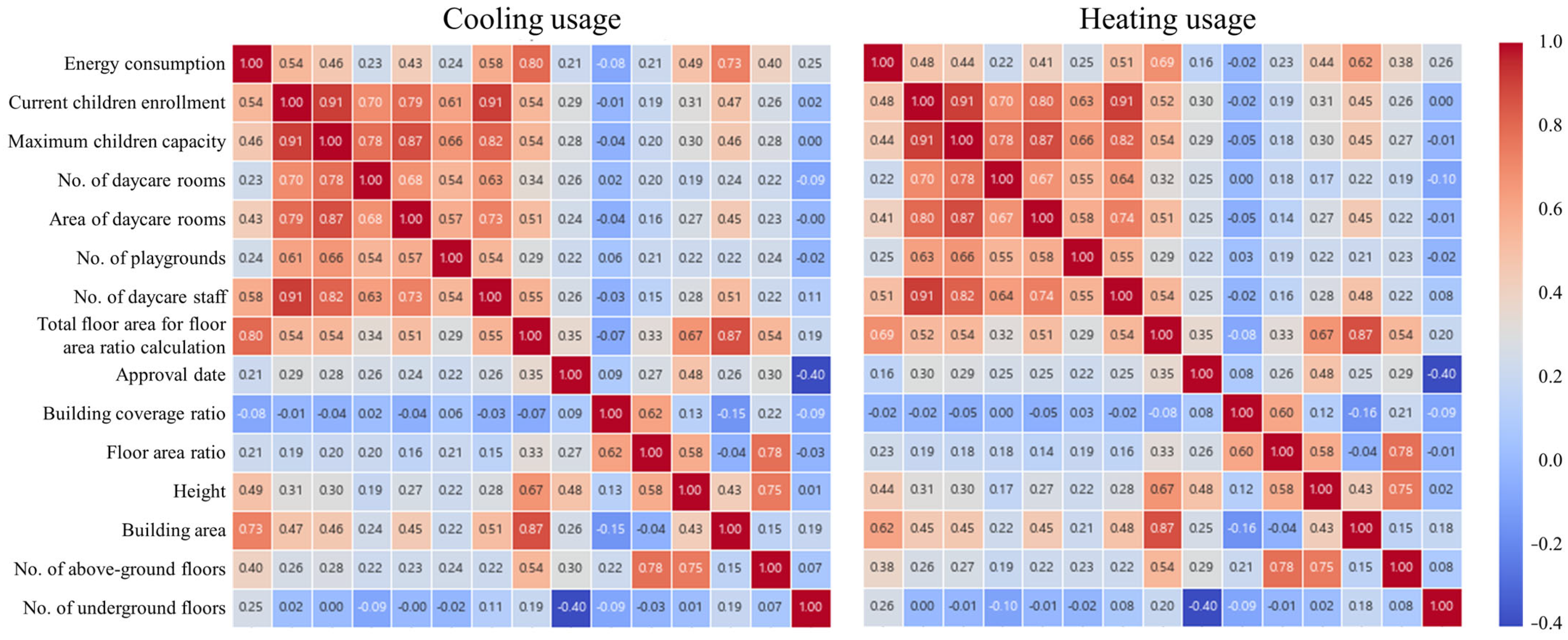
A correlation analysis was performed to examine key factors influencing energy consumption (electricity and city gas). The relationships between the monthly energy consumption and 14 input variables from the collected public data (Table 1) were examined using the Spearman correlation coefficient method. The monthly correlation results for electricity consumption during the summer months (May, June, July, August, and September) and gas consumption during the winter months (January, February, March, November, and December) were obtained. Figure 2 illustrates the monthly average values; positive values indicate a direct relationship between the input and output variables, while negative values represent an indirect relationship. The physical attributes of the buildings, such as floor area, building size, and building height, exerted the greatest influence on energy consumption. Other moderately influential factors included the number of day-care staff and building height, both showing consistent positive correlations. In contrast, the building coverage ratio showed a negative correlation, indicating an indirect relationship; however, it had minimal influence, with correlations close to zero. The GFA for FAR calculation had the strongest impact on energy consumption. Consequently, this study adopted it as the basis for normalizing energy consumption data. In other words, each monthly energy consumption value was divided by the corresponding GFA for FAR to obtain a more intuitive variable.
Figure 3 depicts the normalized annual electricity and gas usage per GFA for FAR calculation in 2018 and 2019. The data from all buildings (Table 2) were averaged by day-care center type. Evidently, the normalized energy usage is relatively consistent across different organizational types of day-care centers. Moreover, discrepancies between 2018 and 2019, mainly due to weather conditions, are evident in Figure 4 and Table 3. During the cooling season in 2018, the OAT, solar radiation, and precipitation were higher, leading to increased cooling energy usage. Conversely, during the heating season in 2018, the OAT and solar radiation were lower, while the precipitation was higher, resulting in increased heating energy consumption. This underscores the importance of incorporating weather variables into the development of evaluation models.

3.1.3. Data Grouping

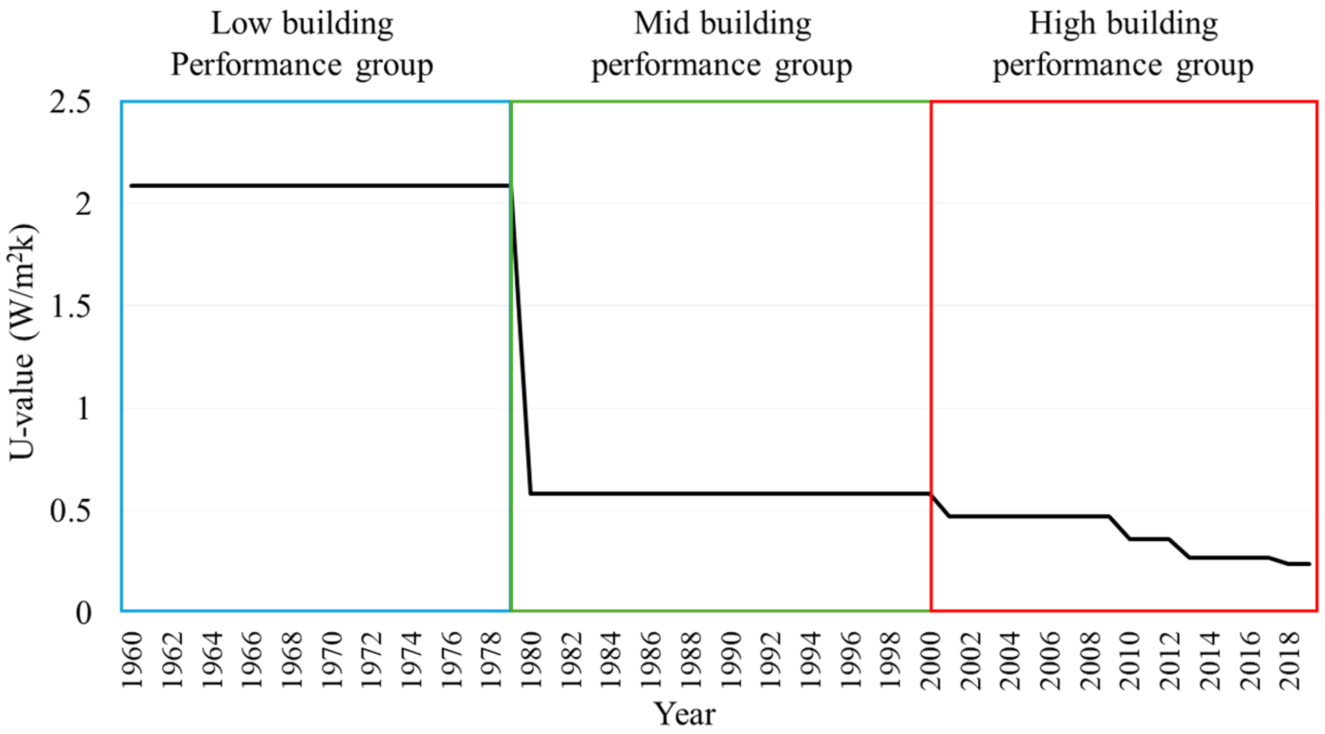
As aforementioned, the normalized data were grouped into three building performance categories—LBP, MBP, and HBP—based on the U-value, an indicator of the thermal transmission efficiency of the building envelope. This value typically decreases as the regulations become increasingly stringent under governmental policy. In South Korea, the U-value remained constant for several decades and was dramatically reduced in 1980. It then remained unchanged for nearly two decades and began to decrease consistently after 2000. This trend is illustrated in Figure 5, which shows the building performance grouping based on the U-values of external walls.
Table 4 presents the grouping results of day-care centers across different efficiency categories, further classified by organizational type. Notably, the number of centers in the LBP group is relatively small compared to those in the other groups. However, the distribution ratios of organizational types within each group are relatively consistent.
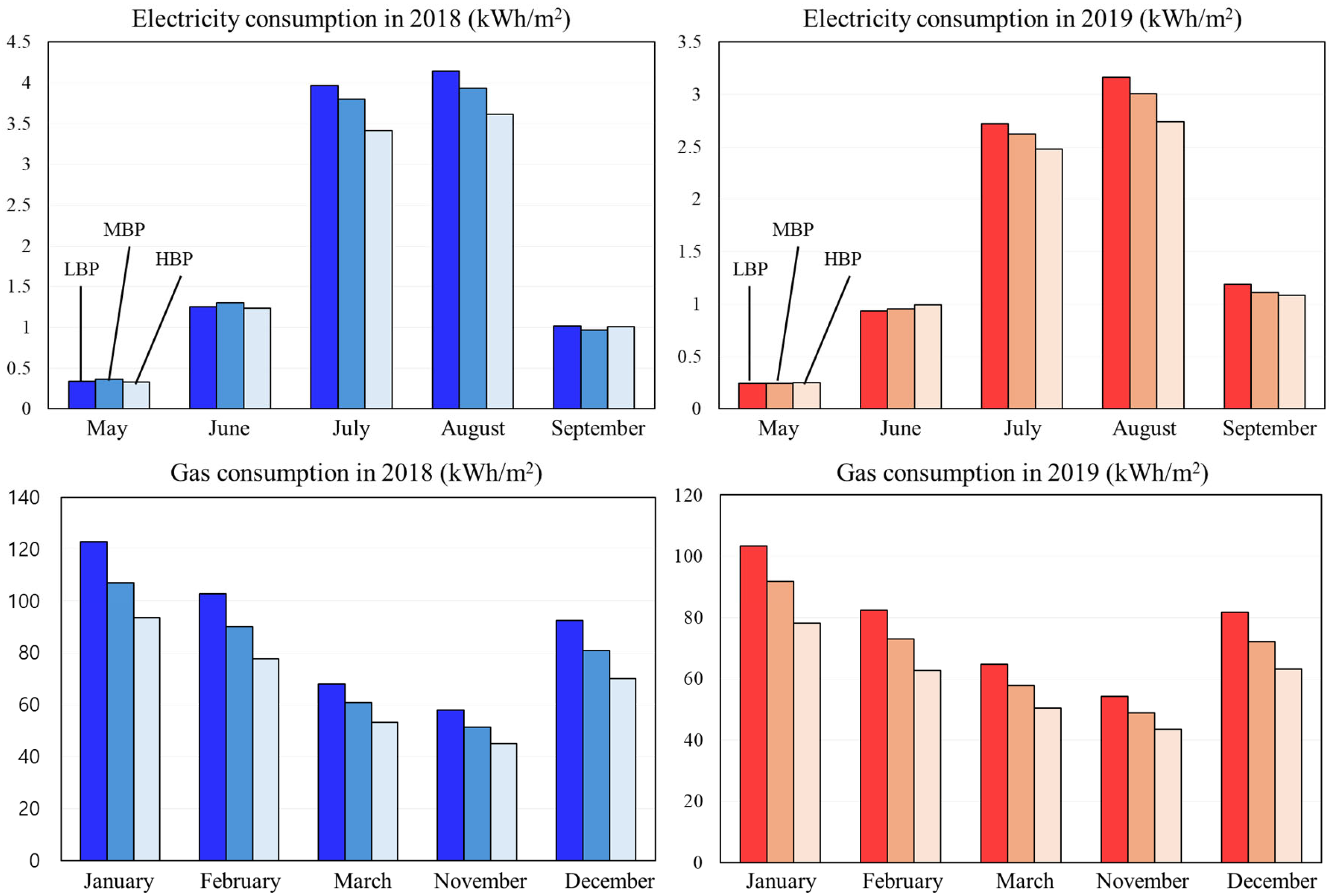
Figure 6 depicts the monthly electricity and gas energy consumption per unit area for each group in 2018 and 2019. As expected, the energy consumption is higher in buildings with lower performance, and vice versa. As regards electricity consumption during the cooling season, this trend is particularly evident in July and August, when the energy usage is significantly higher. However, the trend is relatively less prominent in other months and does not significantly impact the annual cooling energy consumption. In contrast, regarding gas consumption during the heating season, the trend appears more apparent and consistent. These findings justify the incorporation of building performance-related variables, such as thermal transmittance (U-value), into the evaluation model.

3.2. K-Means Clustering for Three Energy Usage Levels: Light, Mid, and Heavy Users

As opposed to the previously described grouping of building energy data based on building performance, this subsection describes the process of clustering each group into three levels of building energy usage—light, mid, and high users. The k-means clustering algorithm, an unsupervised learning algorithm that classifies entities in a dataset into k groups based on shared characteristics, was employed. In this study, the number of clusters was fixed at three. Table 5 presents the hyperparameters of k-means clustering.
The clustering proceeds in the following steps:
  • Initialization Step: The first step in k-means clustering involves selecting k initial centroids. In this study, the k-means++ method was adopted with k fixed at 3; this minimizes the performance degradation caused by the randomness in centroid selection.
  • Assignment Step: In this step, for each data point xi, the distance to each centroid μk is calculated, and the data point is assigned to the cluster with the nearest centroid. The Euclidean distances between each data point and the centroids are computed to identify the closest centroid, and the point is assigned accordingly, as expressed in Equation (1).
C i = a r g m i n k x i u k 2
Here, C i is the index of the cluster to which the data point belongs, and x i u k 2 is the squared Euclidean distance between the data point and centroid.
3.
Update Step: A new centroid is determined based on the mean position of the data points assigned to each cluster. Specifically, the new centroid for each cluster k is set to the mean of the data points within that cluster, as expressed in Equation (2).
u k = 1 C k i C k x i
Here, C K denotes the number of data points in cluster k.
4.
Iteration Step: The assignment and update steps are repeated until the centroid positions no longer change or a predefined number of iterations is reached. This iterative process continues until either the convergence criteria are met or the maximum number of iterations is reached.
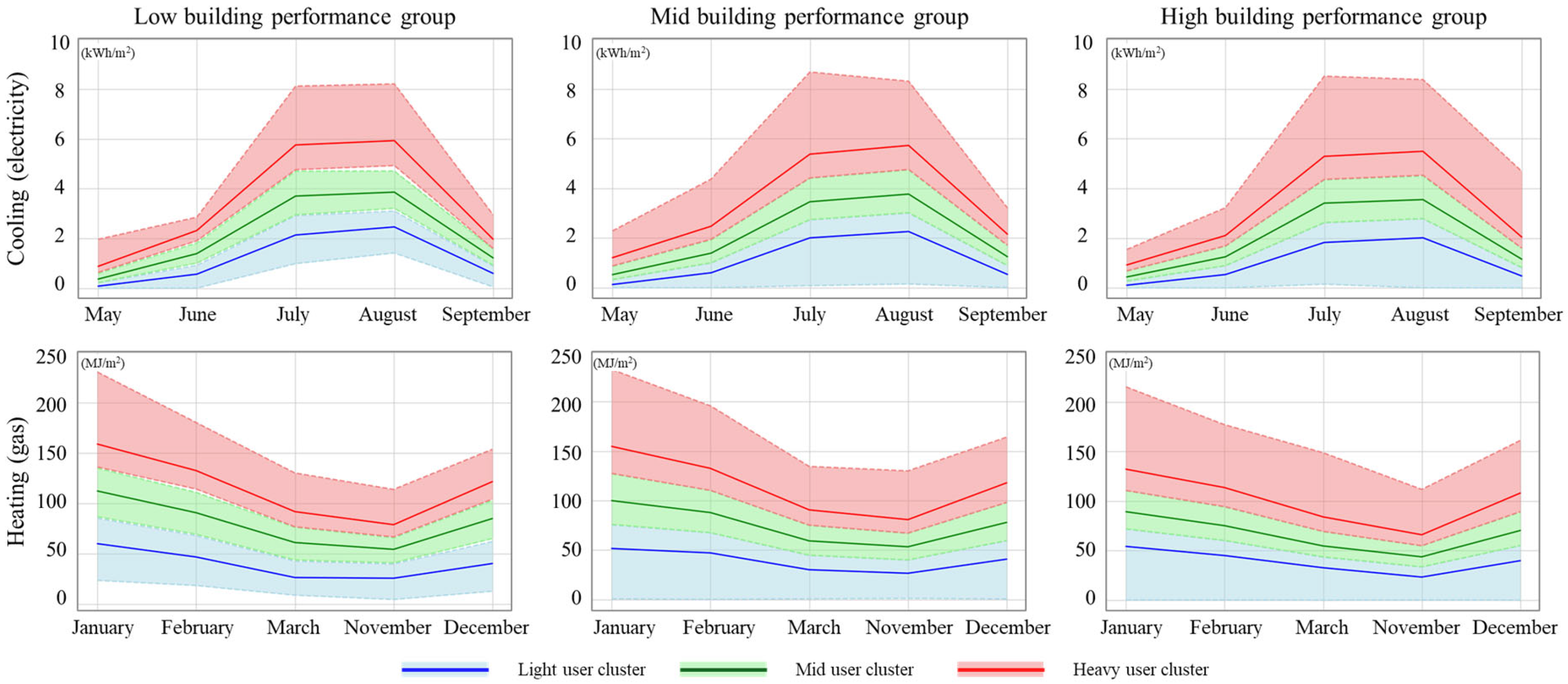
Figure 7 depicts the results of the clustering. The top three plots show the results for electricity consumption, while the bottom three show those for gas consumption. The colors red, green, and blue represent higher, mid, and light users, respectively. The shaded areas indicate the clustered data points, while the lines represent the average trajectories of the clusters. We pre-processed the data by applying the IQR (Interquartile Range) and averaged them to find the representative monthly trajectory of each cluster. While the median can be considered, in most cases, the data is not evenly distributed in each cluster, so the average value can be more representative.
The clustering results were evaluated using the silhouette coefficient. It essentially compares the similarity of each data point within its assigned cluster to its similarity with the nearest neighboring cluster [50]. Within a clustered dataset, the silhouette coefficient is derived by measuring intra-cluster similarity and the inter-cluster similarity for each data point. The average distance between a data point and all other points within the same cluster is defined as a ( i ) , representing internal similarity, that is, how well the data point fits within its cluster. Additionally, the average distance between data point i and all points in the nearest neighboring cluster is defined as b ( i ) , representing external similarity. The silhouette coefficient is then calculated as
s i = b i a ( i ) max a i , b i
s i ranges between −1 and 1 and is calculated based on the following conditions:
i = 1 a i b i ,     a i < b ( i ) 0 ,     a i = b ( i ) a ( i ) b ( i ) 1 ,     a ( i ) > b ( i )
Table 6 presents the silhouette scores for the clustering conducted within each building performance group. All scores were above 0.5 with a minimum at 0.52, a maximum at 0.65, and an average at 0.57, indicating that the clusters are reasonably well formed.

3.3. Evaluation Model Development

This subsection describes the process of developing the evaluation models of building energy usage. The modeling is based on the averaged monthly trajectories of energy usage in each cluster. This entails the use of input variables related to the building performance, building characteristics, and weather condition. LR and various machine-learning models including ANN, RF, and SVR were examined.

3.3.1. Linear Regression

LR yields a polynomial function wherein each input variable is multiplied by a coefficient to be estimated. LR is a fundamental technique in statistics used to model the relationship between input and output variables. It affords insights into the influence of one or more input (independent) variables on the output (the dependent variable). As the number of data points is greater than the number of input variables, the pseudo-inverse matrix method was used Equation (5).
Y = A T A 1 A T X = A + X
Here, X represents the matrix of dependent variables, and Y represents the independent variable vector. The matrix A + can be used to estimate model parameters when the original matrix is non-invertible. The regression coefficients are calculated using A + .
Equation (6) presents the linear model with input and output variables.
Q = c 0 + c 1 · K + c 2 · T + c 3 · P + c 4 · S + c 5 · α + c 6 · β + c 7 · γ
Here, Q is the energy consumption for a specific month; c is the model coefficient, K is the U-value (W/m2K); T is the monthly averaged OAT (℃); P is the monthly total precipitation (mm); S is the monthly total solar radiation (MJ/m2); α is the maximum children enrolment (number); β is the day-care room area (m2); and γ is the number of day-care staff.
The linear model can be presented in matrix form, as shown in Equation (7). Only the cooling case with electricity consumption is presented herein; the heating case is constructed similarly by replacing months 5 to 9 with months 1, 2, 3, 11, and 12. Moreover, the same structure is applied for each building energy usage level (light, mid and heavy user cluster). The vector on the left-hand side represents the monthly cooling energy consumption for different building performance groups (LBP, MBP, and HBP) in 2018 and 2019. On the right-hand side, the coefficient vector is multiplied by the input matrix, which consists of variables related to building performance (e.g., K), weather conditions (e.g., T, P, and S), and building characteristics ( α , β , and γ ). The coefficients are calculated using the pseudo-inverse matrix method for each user group in both heating and cooling cases; the results are presented in Table 7.
Q L B P 5,18 Q L B P 9,18 Q M B P 5,18 Q M B P 9,18 Q H B P 5,18 Q H B P 9,18 Q L B P 5,19 Q L B P 9,19 Q M B P 5,19 Q M B P 9,19 Q H B P 5,19 Q H B P 9,19 = c 0 c 1 c 2 c 7 1 K L B P T L B P , 5,18 P L B P , 5,18 S L B P , 5,18 α L B P β L B P γ L B P     1 K L B P T L B P , 9,18 P L B P , 9,18 S L B P , 9,18 α L B P β L B P γ L B P   1 K M B P T M B P , 5,18 P M B P , 5,18 S M B P , 5,18 α M B P β M B P γ M B P     1 K M B P T M B P , 9,18 P M B P , 9,18 S M B P , 9,18 α M B P β M B P γ M B P     1 K H B P T H B P , 5,18 P H B P , 5,18 S H B P , 5,18 α H B P β H B P γ H B P     1 K H B P T H B P , 9,18 P H B P , 9,18 S H B P , 9,18 α H B P β H B P γ H B P     1 K L B P T L B P , 5,19 P L B P , 5,19 S L B P , 5,19 α L B P β L B P γ L B P     1 K L B P T L B P , 9,19 P L B P , 9,19 S L B P , 9,19 α L B P β L B P γ L B P   1 K M B P T M B P , 5,19 P M B P , 5,19 S M B P , 5,19 α M B P β M B P γ M B P     1 K M B P T M B P , 9,19 P M B P , 9,19 S M B P , 9,19 α M B P β M B P γ M B P     1 K H B P T H B P , 5,19 P H B P , 5,19 S H B P , 5,19 α H B P β H B P γ H B P     1 K H B P T H B P , 9,19 P H B P , 9,19 S H B P , 9,19 α H B P β H B P γ H B P  
On top of the modeling performance, the significance of each variable was analyzed. The permutation importance, standardized coefficient, and SHAP (Shapley Additive exPlanations) were examined. In all cases, some of the environmental variables, including the OAT and precipitation, have higher importance compared to others. For example, in the case of the light energy users (cooling season), the SHAP of the primary variables (OAT and precipitation) ranged from 0.12~0.68, while the rest of the variables were less than 0.04. Because one of the purposes of this study is to develop the methodology, we preserve those relatively less significant variables of building characteristics (maximum children enrolment, day-care room area, and number of day-care staff). When applied to others building types, those characteristics can be set differently according to the target building.

3.3.2. Artificial Neural Networks (ANN) Model

The ANN is a machine learning model inspired by the structure of biological neural networks, as illustrated in Figure 8. This model is composed of an input layer, one or more hidden layers, and an output layer, mirroring the interconnected structure of neurons. Each neuron processes inputs by applying a weighted sum and activation function, enabling the model to capture complex, nonlinear relationships within the data. Table 8 presents the hyperparameter settings for the ANN used in this study. The bounds of the number and size of the hidden layer were set to 1–3 and 2–30, respectively, with the final values determined via hyperparameter optimization.

3.3.3. Random Forest Model

RF is an ensemble learning method that combines multiple decision trees to enhance the accuracy and stability of predictions. Each tree in the forest is trained on a random subset of the data. For regression tasks, the final prediction is obtained by averaging the predictions of all trees, while for classification tasks, it is determined by majority voting. This method can effectively reduce the risk of overfitting and improve model stability. The hyperparameter settings for RF are presented in Table 9. The number of trees, leaf size, and number of splits were set to 2–30, 1–5, and 10–50, respectively. The final values obtained through hyperparameters optimization are also presented.

3.3.4. Support Vector Regression Model

SVR is a widely used machine learning technique for regression analysis, used to predict target values from input data. SVR performs classification or prediction by mapping the input data into a high-dimensional space, as illustrated in Figure 9, where it constructs a hyperplane that serves as the regression function. This hyperplane, existing in a higher dimensional space, is used to estimate target values based on the input variables. To perform regression in this high-dimensional space, SVR employs a kernel function, a function that maps data points onto the higher dimension. Common types of kernels include the sigmoid, polynomial, and Gaussian kernels; the choice of the kernel significantly affects the model’s performance, depending on the characteristics of the data. Surrounding the hyperplane are boundary lines, which are positioned at distances of ε (margin of tolerance) from the hyperplane. These lines allow a tolerable range of errors in the prediction process, and the precision of the model is influenced by these margins. Lastly, the data points that lie close to or on the boundary lines are referred to as support vectors and play a pivotal role in defining the hyperplane. These vectors, determined through optimization, are critical to the SVR model as they establish the hyperplane position and orientation. The SVR hyperparameter settings employed in this study are shown in Table 10. A linear or Gaussian kernel was considered. The range of kernel scale, box constraints, and epsilon value were set to 1–10, 10–100, and 0.1–0.5, respectively. The final values were determined via hyperparameter optimization.

3.3.5. Modeling Performance Analysis

The results obtained using the LR and machine-learning methods were evaluated using three statistical criteria, namely, R2, RMSE, and cv(RMSE). R2, the coefficient of determination, is a metric that indicates how well the regression model explains the variability of the data (Equation (8)). A value closer to 1 suggests that the model effectively explains the variability in the data. The numerator in Equation (8) represents the residual sum of squares (RSS), which measures the error in the model’s predictions, while the denominator represents the total sum of squares (TSS), which indicates the total variability in the data [51]. RMSE is a commonly used metric for evaluating model performance, representing the square root of the squared differences between predicted and actual values (Equation (9)) [52]. cv(RMSE) expresses the RMSE as a percentage of the mean actual value, allowing for a relative evaluation of the model’s prediction error (Equation (10)). By standardizing RMSE to the mean, cv(RMSE) facilitates the comparison of predictive performance across datasets of varying scales. It indicates how large the prediction error is relative to the average value of the data, with a lower value implying higher prediction accuracy. This metric is typically used for evaluating the calibration performance of building energy modeling [53].
In the following equations, n is total number of data points, y i is the actual data value, y i ^   is the predicted value, and y i ¯   is the mean of the actual data values.
R 2 = i = 1 n ( y i y i ^ ) 2 i = 1 n ( y i y ¯ ) 2
R M S E = 1 n i = 1 n ( y i y i ^ ) 2
C V R M S E = 1 y i ¯ × 1 n i = 1 n ( y i y i ^ ) 2
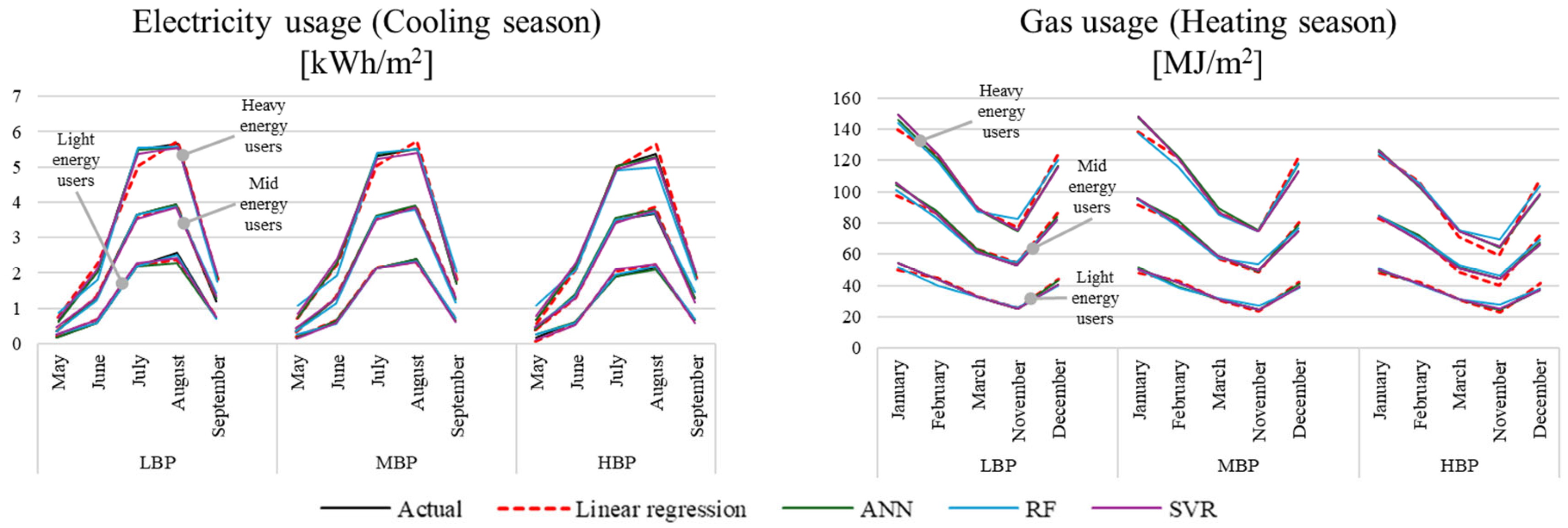
Table 11 and Table 12 present the R2, RMSE, and cv(RMSE) values for the developed models, while the trajectories are shown in Figure 10. Evidently, reasonable performances were achieved for all models across different criteria. This is because the number of data (averaged from cluster in each building performance group) is not many—e.g., the number of columns in the matrix in Equation (7) is only seven. This can be extended if more yearly data are used for modeling. The LBP group showed relatively low model performance for both seasonal models. This may be attributed to the limited amount of test data available for the LBP group; the data proportion of the LBP group is approximately 20%, which is substantially lower than those of other building performance groups (see Table 4).
In all cases, the modeling performance of the LR model is slightly lower compared to that of the machine learning models. This is because the latter models can capture the nonlinear relationship between the input variables and output, while LR only reflects the linear relationship. However, machine learning models may not be widely adopted due to their complexity. For example, they cannot be easily implemented into policymaking processes by governments or decision-makers. Conversely, the linear model is more suitable for practical applications as it can be directly used given the model structure and the derived coefficients.

3.4. Virtual Demonstration with Example Cases

A virtual demonstration was performed considering example cases. Three building data from the 2018 open dataset in the public sector were extracted for the demonstration, focusing on the cooling case. In the first case, the building was constructed in 1995–1996, and its U-value was 0.58 W/m2K. The monthly average OAT values were 18.2, 23.1, 27.8, 28.8, and 21.5 °C. The monthly total precipitation values were 222, 171.5, 185.6, 202.6, and 68.5 mm. The monthly total solar radiation values were 561, 603, 561, 517, and 471 MJ/m2. The maximum children enrolment, day-care room area, and number of day-care staff were 101 children, 316 m2, and 23 people, respectively. The estimated coefficients of the linear model presented in Table 7 were multiplied by these input variables, and the monthly energy consumptions were derived for heavy, mid, and light user groups. The trajectories of the second and third examples were drawn in the same manner.
Table 13 and Figure 11 present the results of the example cases. This actual monthly energy usage is compared to the three trajectories of heavy, mid, and light users. By computing the RMSE, the users’ energy level is evaluated: for example, the building energy user is categorized at the specific level corresponding to the trajectory with the minimum RMSE. The user considered in example 1 is thus identified as a mid user while that of example 3 is identified as a light user. Compared to those two examples, example 2 is not clear based on the observation of the trajectories in Figure 11, but it was found to be the heavy user by the RMSE comparison between the actual usage and three clustered trajectories.

4. Conclusions

This study developed a methodology for evaluating building energy usage based on the actual energy consumption data from governmental institutions. A case study was then conducted on day-care centers in South Korea by applying the proposed methodology. First, actual building energy data were normalized using GFA for FAR calculation, which showed the greatest impact among all input variables. The data were then grouped according to the building performance (e.g., U-value). Second, monthly building energy data for electricity (cooling season) and gas (heating season) were clustered into three energy usage levels, namely, heavy, mid, and light users. Third, evaluation models were developed using LR and machine learning methods including ANN, RF, and SVR, and the monthly energy trajectories for each usage level were derived based on inputs such as performance, weather, and building characteristics. The main findings of the study are summarized as follows:
  • Clustering for building energy usage levels was carried out based on actual energy consumption data from day-care center buildings. Heavy user, mid user, and light user groups were identified with reasonable reliability by using the k-means clustering method.
  • Regression and machine-learning-based models were developed for each cluster, with inputs including building performance (U-value), weather, building characteristics, and output of monthly energy consumption. All models showed reasonable performance (12% cv(RMSE) in the worst case); the LR model is recommended for practical use owing to its simplicity and applicability to policy and decision-making.
  • The evaluation process was demonstrated through virtual examples. To this end, three trajectories of building energy usage levels, calculated using the input variables and the coefficients of the linear model, were compared with the actual monthly energy consumption trajectory.

5. Discussion and Limitations

The simplified LR model is designed to aid policy formulation and decision-making processes for end users by providing actionable insights into consumption patterns. The developed models classify users based on their electricity and gas consumption levels, identifying light, mid, and heavy users. This classification enables policymakers and decision-makers to implement targeted strategies, such as incentivizing energy-efficient behavior among light users or imposing restrictions or penalties on heavy users. However, this study has several inevitable limitations, which are summarized as follows, along with future work suggestions:
Data deficiency: Only the building energy data from entire buildings occupied by day-care centers were used. This limitation resulted from privacy concerns, as only aggregated building-level energy data are collected by the government. In the future, if the government initiates the collection of more granular energy data, more detailed and extensive analyses would be feasible. For example, thermostat and setpoint temperature data as well as the schedule of the occupants might be acquired. Moreover, this study manually grouped the building data according to the building performance, thereby the number of data is different in each group. This might degrade the modeling performance of the evaluation models. A more extensive dataset is required to resolve this potential issue regarding the data imbalance.
Generalization of methodology: This study focused on day-care center buildings as a case study. However, the public data used may not fully reflect the diversity of building types and energy consumption patterns. The dataset primarily represents specific regions and building categories, limiting the generalizability of the findings to other regions with different climates or construction practices. Future research should seek to improve the robustness and applicability of the models by incorporating data from various geographic locations and building types.
Weather impact: The analysis in this study revealed a clear correlation between the weather variables and energy consumption. However, this study used only two years of energy consumption data. To improve the applicability of the model, future studies should include datasets with longer time periods and more diverse weather profiles.
Metacognition: The long-term target of this study is to induce the building energy usage through metacognition. This study does not explain the clear linkage between the users’ behaviors and labeling the energy usage level. However, future studies might investigate the apparent metacognition process by evaluating the energy usage evaluation and corresponding energy-saving behavior.

Author Contributions

Conceptualization, J.J. and D.-W.K.; methodology, J.J. and D.-W.K.; software, J.P.; validation, J.P., K.C. and C.-H.M.; formal analysis, A.T.; investigation, S.P.; resources, J.J.; data curation, S.P.; writing—original draft preparation, J.P. and J.J.; writing—review and editing, J.J.; visualization, K.C.; supervision, J.J.; project administration, J.J.; funding acquisition, D.-W.K. All authors have read and agreed to the published version of the manuscript.

Funding

This work is supported by the Korea Agency for Infrastructure Technology Advancement (KAIA) grant funded by the Ministry of Land, Infrastructure and Transport (Grant RS-2023-00244769).

Institutional Review Board Statement

Not applicable.

Informed Consent Statement

Not applicable.

Data Availability Statement

The data can not be shared.

Conflicts of Interest

Author Jinhyung Park is from EG Solutions. The remaining authors declare that the research was conducted in the absence of any commercial or financial relationships that could be construed as a potential conflict of interest.

Nomenclature

Description and Units of Symbols
SymbolDescriptionUnit
c Coefficient derivation-
C k Number of data points in cluster k-
iIndex-
KThermal transmittanceW/m2°C
nTotal number of data points-
PPrecipitationMm
s ( i ) Silhouette coefficient score-
SSolar radiationw/m2
TOutdoor air temperature
u k Distance from the centroid-
x i Position of a data point-
XIndependent variable matrix-
YDependent variable matrix-
yMeasured data valueskWh, MJ
α Maximum children enrollmentNo.
β Day-care room aream2
β ^ Estimated regression coefficients-
γ Number of day-care staffNo.

Abbreviations

ANNArtificial neural network
FARFloor area ratio
GFAGross floor area
HVACHeating, ventilation, and air-conditioning
HBPHigh building performance
LBPLow building performance
MBPMid building performance
RFRandom forest
RMSERoot mean square error
SVRSupport vector regression
TOUTime of use
OATOutdoor air temperature

Subscripts and Superscripts

elecElectricity
gasGas
Mean function
TInverse function
Predicted/estimated function

Appendix A

Table A1. Public institution for domestic building energy data in South Korea.
InstitutionPlatform NameProvided Data
Korea Energy AgencyBuilding Energy Service Total Platform-Explanation of building energy systems and civil complaint services
-Statistics on building attributes, energy sources
-Total energy consumption assessment, building operation efficiency
Ministry of Land, Infrastructure and TransportArchitectural Data Open System-Monthly electricity and gas energy consumption by lot number
Apartment Complex Management Information System-Monthly and yearly statistics on heating, hot water, gas, electricity, water energy usage costs, and energy consumption by apartment complex
Public Building Energy Consumption Information Management System-Monthly energy consumption of public buildings
Building Energy Consumption Map-Annual energy consumption by energy source and detailed use for each city and province
Korea Electric Power CorporationEnergy Integrated Platform-Status of electricity, water, gas, heating energy by district in the pilot city, and renewable energy generation status
Ministry of the Interior and SafetyPublic Data Portal-Greenhouse gas emissions from local government buildings
-Building energy efficiency rating information
-Energy consumption by building (electricity, gas) by lot number
-Energy usage information of apartment complexes
-Energy consumption by energy source, energy statistics
Korea Institute of Energy Technology Evaluation and PlanningDevelopment and Establishment of a Housing Energy Big Data Platform-Data under development
Table A2. Monthly correlation coefficients for the variables.
2018 Electricity2019 Electricity2018 Gas2019 Gas
May.Jun.Jul.Aug.Sep.May.Jun.Jul.Aug.Sep.Jan.Feb.Mar.Nov.Dec.Jan.Feb.Mar.Nov.Dec.
Current children enrollment0.480.490.550.520.530.470.510.540.50.540.430.450.50.30.430.390.430.50.20.48
Maximum children enrollment0.410.410.470.450.480.40.430.460.430.470.410.470.470.280.40.380.470.470.140.44
Number of day-care rooms0.170.180.240.20.220.170.20.230.20.220.170.250.260.080.190.140.240.2300.22
Area of day-care rooms0.40.40.450.430.450.380.40.430.40.430.370.450.450.280.390.340.430.430.130.41
Number of playgrounds0.220.230.270.240.270.210.230.240.20.250.170.240.240.120.210.180.250.240.020.25
Number of day-care staff0.50.520.570.550.560.530.550.580.550.570.450.490.520.360.470.430.490.520.260.51
GFA for FAR calculation0.770.760.770.780.770.810.810.80.810.80.690.720.730.570.690.680.720.760.460.69
Approval date0.230.220.240.230.240.210.220.210.20.220.20.210.270.140.180.130.170.240.040.16
Building coverage ratio−0.08−0.06−0.05−0.05−0.07−0.1−0.09−0.08−0.09−0.07−0.03−0.01−0.04−0.05−0.02−0.01−0.04−0.06−0.01−0.02
Floor area ratio0.190.20.230.210.20.180.20.210.20.210.180.230.180.120.20.220.220.20.170.23
Building height0.450.440.480.460.440.480.480.490.490.470.440.480.480.350.450.440.460.50.330.44
Building area0.750.720.710.740.740.760.750.730.740.750.670.670.710.550.640.630.640.70.410.62
No. of above-ground floor0.330.350.390.360.330.360.380.40.390.370.350.380.350.260.350.380.410.390.260.38
No. of underground floors0.250.250.240.260.230.280.260.250.280.270.220.190.170.250.240.250.240.220.270.26

References

  1. IEA. Energy Efficiency 2023; IEA: Paris, France, 2023; Available online: https://www.iea.org/reports/energy-efficiency-2023 (accessed on 14 September 2025).
  2. IRENA. World Energy Transitions Outlook; IRENA: Abu Dhabi, United Arab Emirates, 2023; Available online: https://www.iea.org/reports/world-energy-outlook-2023 (accessed on 14 September 2025).
  3. European Commission. European Green Deal: Energy Efficiency Directive Adopted, Helping Make the EU ‘Fit for 55′; European Commission: Brussels, Belgium, 2023; Available online: https://energy.ec.europa.eu/news/european-green-deal-energy-efficiency-directive-adopted-helping-make-eu-fit-55-2023-07-25_en (accessed on 14 September 2025).
  4. US Environmental Protection Agency. Energy Star Program Overview; US Environmental Protection Agency: Washington, DC, USA, 2023.
  5. Laaroussi, Y.; Bahrar, M.; el Mankibi, M.; Draoui, A.; Si-Larbi, A. Occupant presence and behavior: A major issue for building energy performance simulation and assessment. Sustain. Cities Soc. 2020, 63, 102420. [Google Scholar] [CrossRef]
  6. Crawley, D.B.; Lawrie, L.K.; Winkelmann, F.C.; Buhl, W.F.; Huang, Y.J.; Pedersen, C.O.; Strand, R.K.; Liesen, R.J.; Fisher, D.E.; Witte, M.J.; et al. EnergyPlus: Creating a new-generation building energy simulation program. Energy Build. 2001, 33, 319–331. [Google Scholar] [CrossRef]
  7. TRNSYS (A TRaNsient SYstems Simulation Program). Available online: https://trnsys.org/ (accessed on 14 September 2025).
  8. Prototype Building Models. Available online: https://www.energycodes.gov/prototype-building-models (accessed on 14 September 2025).
  9. BPD (Building Performance Database). Department of Energy, United States. 2014. Available online: https://bpd.lbl.gov (accessed on 14 September 2025).
  10. Granderson, J.; Lin, G.; Chen, Y.; Casillas, A.; Wen, J.; Chen, Z.; Im, P.; Huang, S.; Ling, J. A labeled dataset for building HVAC systems operating in faulted and fault-free states. Sci. Data 2023, 10, 342. [Google Scholar] [CrossRef] [PubMed]
  11. Na, W.; Liu, S. Benchmarking building energy consumption for space heating using an empirical Bayesian approach with urban-scale energy model. Energy Build. 2024, 320, 114581. [Google Scholar] [CrossRef]
  12. Yoon, Y.; Jung, S.; Im, P.; Gehl, A. Datasets of a Multizone Office Building under Different HVAC System Operation Scenarios. Sci. Data 2022, 9, 775. [Google Scholar] [CrossRef] [PubMed]
  13. Arjunan, P.; Poolla, K.; Miller, C. BEEM: Data-driven building energy benchmarking for Singapore. Energy Build. 2022, 260, 111869. [Google Scholar] [CrossRef]
  14. Li, T.; Bie, H.; Lu, Y.; Sawyer, A.O.; Loftness, V. MEBA: AI-powered precise building monthly energy benchmarking approach. Appl. Energy 2024, 359, 122716. [Google Scholar] [CrossRef]
  15. Park, H.S.; Lee, M.; Kang, H.; Hong, T.; Jeong, J. Development of a new energy benchmark for improving the operational rating system of office buildings using various data-mining techniques. Appl. Energy 2016, 173, 225–237. [Google Scholar] [CrossRef]
  16. Luo, N.; Wang, Z.; Blum, D.; Weyandt, C.; Bourassa, N.; Piette, M.A.; Hong, T. A three-year dataset supporting research on building energy management and occupancy analytics. Sci. Data 2022, 9, 156. [Google Scholar] [CrossRef]
  17. Lee, K.; Lim, H.; Hwang, J.; Lee, D. Development of building benchmarking index for improving gross-floor-area-based energy use intensity. Energy Build. 2025, 328, 115103. [Google Scholar] [CrossRef]
  18. Piscitelli, M.S.; Giudice, R.; Capozzoli, A. A holistic time series-based energy benchmarking framework for applications in large stocks of buildings. Appl. Energy 2024, 357, 122550. [Google Scholar] [CrossRef]
  19. Piscitelli, M.S.; Razzano, G.; Buscemi, G.; Capozzoli, A. An interpretable data analytics-based energy benchmarking process for supporting retrofit decisions in large residential building stocks. Energy Build. 2025, 328, 115115. [Google Scholar] [CrossRef]
  20. Roth, J.; Lim, B.; Jain, R.K.; Grueneich, D. Examining the feasibility of using open data to benchmark building energy usage in cities: A data science and policy perspective. Energy Policy 2020, 139, 111327. [Google Scholar] [CrossRef]
  21. Liu, C.; Li, Y.; Chen, H.; Xing, L.; Zhang, S. Energy-saving potential benchmarking method of office buildings based on probabilistic forecast. J. Build. Eng. 2024, 95, 110282. [Google Scholar] [CrossRef]
  22. Zheng, P.; Zhou, H.; Liu, J.; Nakanishi, Y. Interpretable building energy consumption forecasting using spectral clustering algorithm and temporal fusion transformers architecture. Appl. Energy 2023, 349, 121607. [Google Scholar] [CrossRef]
  23. Piselli, C.; Pisello, A.L. Occupant behavior long-term continuous monitoring integrated to prediction models: Impact on office building energy performance. Energy 2019, 176, 667–681. [Google Scholar] [CrossRef]
  24. Nazeriye, M.; Haeri, A.; Haghighat, F.; Panchabikesan, K. Understanding the influence of building characteristics on enhancing energy efficiency in residential buildings: A data mining based study. J. Build. Eng. 2021, 43, 103069. [Google Scholar] [CrossRef]
  25. Kim, H.; Ham, S.; Promann, M.; Devarapalli, H.; Bihani, G.; Ringenberg, T.; Kwarteng, V.; Bilionis, I.; Braun, J.E.; Rayz, J.T.; et al. MySmartE—An eco-feedback and gaming platform to promote energy conserving thermostat-adjustment behaviors in multi-unit residential buildings. Build. Environ. 2022, 221, 109252. [Google Scholar] [CrossRef]
  26. Kim, H.; Bilionis, I.; Karava, P.; Braun, J.E. Human decision making during eco-feedback intervention in smart and connected energy-aware communities. Energy Build. 2023, 278, 112627. [Google Scholar] [CrossRef]
  27. Zhu, J.; Shen, Y.; Song, Z.; Zhou, D.; Zhang, Z.; Kusiak, A. Data-driven building load profiling and energy management. Sustain. Cities Soc. 2019, 49, 101587. [Google Scholar] [CrossRef]
  28. Trotta, G. An empirical analysis of domestic electricity load profiles: Who consumes how much and when? Appl. Energy 2020, 275, 115399. [Google Scholar] [CrossRef]
  29. Ciulla, G.; D’Amico, A. Building energy performance forecasting: A multiple linear regression approach. Appl. Energy 2019, 253, 113500. [Google Scholar] [CrossRef]
  30. Olu-Ajayi, R.; Alaka, H.; Sulaimon, I.; Sunmola, F.; Ajayi, S. Building energy consumption prediction for residential buildings using deep learning and other machine-learning techniques. J. Build. Eng. 2022, 45, 103406. [Google Scholar] [CrossRef]
  31. Shi, Z.; Wu, L.; Zhou, Y. Predicting household energy consumption in an aging society. Appl. Energy 2023, 352, 121899. [Google Scholar] [CrossRef]
  32. Tang, W.; Wang, H.; Lee, X.L.; Yang, H.T. Machine-learning approach to uncovering residential energy consumption patterns based on socioeconomic and smart meter data. Energy 2022, 240, 122500. [Google Scholar] [CrossRef]
  33. Li, X.; Yao, R. A machine-learning-based approach to predict residential annual space heating and cooling loads considering occupant behaviour. Energy 2020, 212, 118676. [Google Scholar] [CrossRef]
  34. Kamel, E.; Sheikh, S.; Huang, X. Data-driven predictive models for residential building energy use based on the segregation of heating and cooling days. Energy 2020, 206, 118045. [Google Scholar] [CrossRef]
  35. Konstantakopoulos, I.C.; Barkan, A.R.; He, S.; Veeravalli, T.; Liu, H.; Spanos, C. A deep learning and gamification approach to improving human-building interaction and energy efficiency in smart infrastructure. Appl. Energy 2019, 237, 810–821. [Google Scholar] [CrossRef]
  36. Wei, P.; Xia, S.; Chen, R.; Qian, J.; Li, C.; Jiang, X. A Deep-Reinforcement-Learning-Based Recommender System for Occupant-Driven Energy Optimization in Commercial Buildings. IEEE Internet Things J. 2020, 7, 6402–6413. [Google Scholar] [CrossRef]
  37. Motlagh, O.; Berry, A.; O’Neil, L. Clustering of residential electricity customers using load time series. Appl. Energy 2019, 237, 11–24. [Google Scholar] [CrossRef]
  38. Zhang, X.; Ramírez-Mendiola, J.L.; Li, M.; Guo, L. Electricity consumption pattern analysis beyond traditional clustering methods: A novel self-adapting semi-supervised clustering method and application case study. Appl. Energy 2022, 308, 118335. [Google Scholar] [CrossRef]
  39. Wang, C.; Du, Y.; Li, H.; Wallin, F.; Min, G. New methods for clustering district heating users based on consumption patterns. Appl. Energy 2019, 251, 113373. [Google Scholar] [CrossRef]
  40. Duan, J.; Li, N.; Peng, J.; Liu, Q.; Peng, T.; Wang, S. Clustering and prediction of space cooling and heating energy consumption in high-rise residential buildings with the influence of occupant behaviour: Evidence from a survey in Changsha, China. J. Build. Eng. 2023, 76, 107418. [Google Scholar] [CrossRef]
  41. Wang, S.; Liu, H.; Pu, H.; Yang, H. Spatial disparity and hierarchical cluster analysis of final energy consumption in China. Energy 2020, 197, 117195. [Google Scholar] [CrossRef]
  42. Yilmaz, S.; Chambers, J.; Patel, M.K. Comparison of clustering approaches for domestic electricity load profile characterisation—Implications for demand side management. Energy 2019, 180, 665–677. [Google Scholar] [CrossRef]
  43. Park, S.H.; Lee, S.M.; Ahn, N.H. A Case Study on Pilot Application of Building Diagnosis Evaluation Method Considering Architectural and Mechanical Elements. J. Korean Inst. Archit. Sustain. Environ. Build. Syst. 2020, 14, 439–450. [Google Scholar] [CrossRef]
  44. Ministry of Land Infrastructure and Transport. Open Service Sector. Available online: https://www.hub.go.kr/portal/main.do (accessed on 14 September 2025).
  45. Korea Meteorological Administration, Automated Synoptic Observing System. Available online: https://data.kma.go.kr/data/grnd/selectAsosRltmList.do;jsessionid=ES0sOzyo9y0irTs93l8JXjm7aCYA6wRNl8Yf7tBbNgzkFavt7C0kRv6ChttkH4Fl.was01_servlet_engine5?pgmNo=36 (accessed on 14 September 2025).
  46. Tahmasebinia, F.; He, R.; Chen, J.; Wang, S.; Sepasgozar, S.M.E. Building Energy Performance Modeling through Regression Analysis: A Case of Tyree Energy Technologies Building at UNSW Sydney. Buildings 2023, 13, 1089. [Google Scholar] [CrossRef]
  47. Saxena, A.; Prasad, M.; Gupta, A.; Bharill, N.; Patel, O.P.; Tiwari, A.; Er, M.J.; Ding, W.; Lin, C.T. A review of clustering techniques and developments. Neurocomputing 2017, 267, 664–681. [Google Scholar] [CrossRef]
  48. Alzubi, J.; Nayyar, A.; Kumar, A. Machine Learning from Theory to Algorithms: An Overview. J. Phys. Conf. Ser. 2018, 1142, 012012. [Google Scholar] [CrossRef]
  49. Jung, S.H.; Kim, J.C.; Kim, C.Y.; Yoo, K.S.; Shim, C.B. A Study on Cluster-based Classification Evaluation Prediction Model for Measuring the Accuracy of Unsupervised Learning Data. J. Korea Multimed. Soc. 2018, 21, 779–786. [Google Scholar]
  50. Rousseeuw, P.J. Silhouettes: A graphical aid to the interpretation and validation of cluster analysis. J. Comput. Appl. Math. 1987, 20, 53–65. [Google Scholar] [CrossRef]
  51. Chong, A.; Augenbroe, G.; Yan, D. Occupancy data at different spatial resolutions: Building energy performance and model calibration. Appl. Energy 2021, 286, 116492. [Google Scholar] [CrossRef]
  52. Hodson, T.O. Root-mean-square error (RMSE) or mean absolute error (MAE): When to use them or not. In Geoscientific Model Development; Copernicus GmbH: Göttingen, Germany, 2022; Volume 15, pp. 5481–5487. [Google Scholar] [CrossRef]
  53. Ruiz, G.R.; Bandera, C.F. Validation of calibrated energy models: Common errors. Energies 2017, 10, 1587. [Google Scholar] [CrossRef]
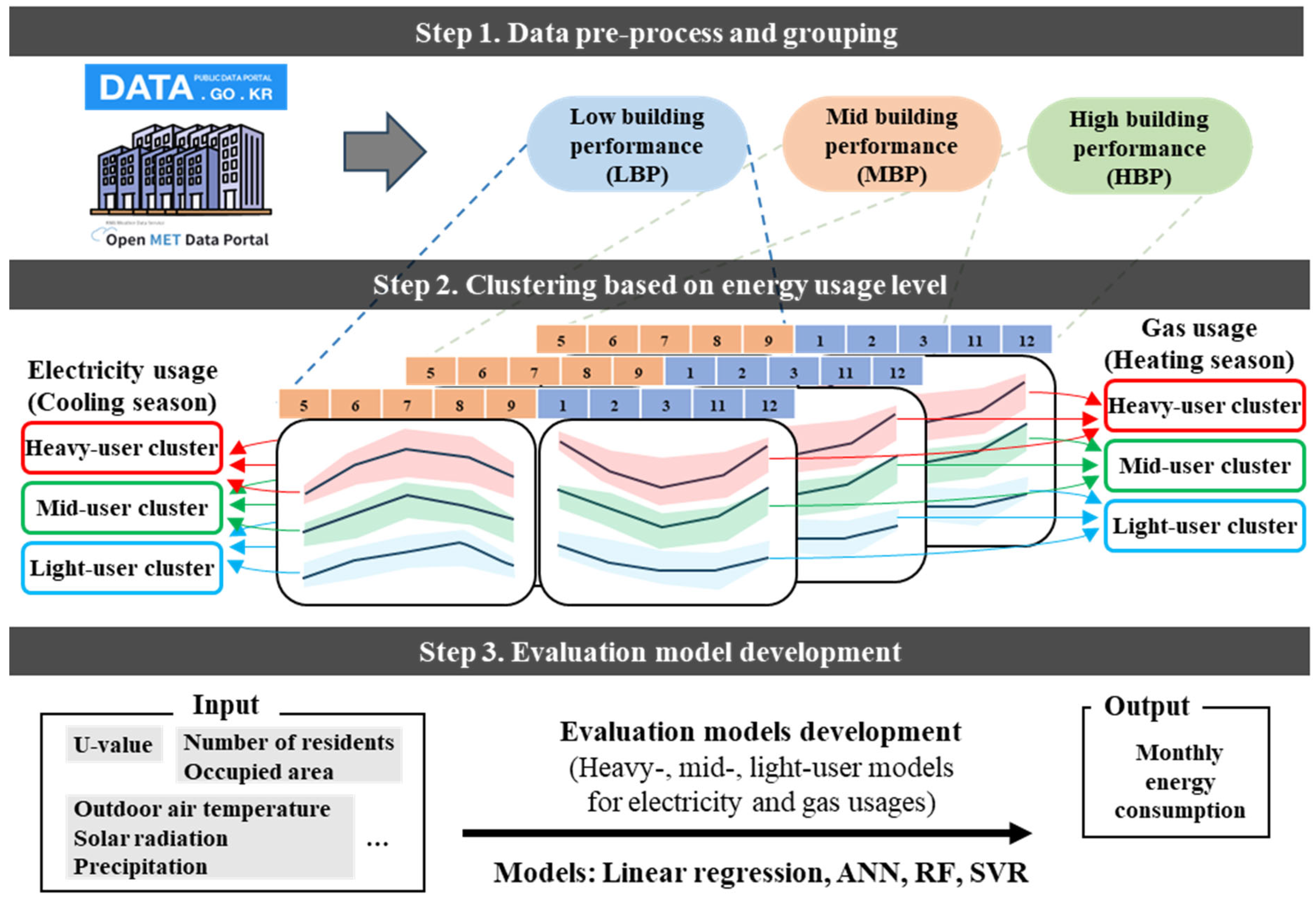
Figure 1. Overview of the proposed methodology.
Sustainability 17 08339 g001
Figure 2. Correlation analysis of input variables.
Sustainability 17 08339 g002
Figure 3. Normalized electricity and gas consumption for each day-care center type.
Sustainability 17 08339 g003
Figure 4. Weather data profiles: box plots (2018 and 2019 with hourly data).
Sustainability 17 08339 g004
Figure 5. Building performance grouping based on thermal transmittance.
Sustainability 17 08339 g005
Figure 6. Electricity and gas energy consumption by each group (low, mid, and high building performance groups).
Sustainability 17 08339 g006
Figure 7. Clustering results of electricity and gas energy consumption patterns (the area represents the data distribution while the trajectories represent the average value).
Sustainability 17 08339 g007
Figure 8. ANN architecture.
Sustainability 17 08339 g008
Figure 9. SVR architecture.
Sustainability 17 08339 g009
Figure 10. Monthly trajectories of actual and modeling results.
Sustainability 17 08339 g010
Figure 11. Evaluation of energy usage levels.
Sustainability 17 08339 g011
Table 1. Collected public data.
CategoryData NameData ScopeData Content
Ministry of Land, Infrastructure and Transport
(Architectural Data Open System)
Building registerBasic overview
General title section
General title section PK *, Title section PK *, Land address, Approval date, Building area, Gross floor area (GFA) for floor area ratio (FAR) calculation, Building coverage ratio, Gross floor area (GFA), Number of above-ground floors, Number of underground floors, Main use code, Other use code, Number of households, etc.
Monthly energy usageElectricity usage
Gas usage
Usage year and month, Usage purpose code, Supply institution code, Monthly energy consumption
Ministry of Health and Welfare
(Day-care Centers)
Day-care center information disclosure portalSeoul, South KoreaDay-care center type, Address, Number of day-care rooms, Area of day-care rooms, Number of playgrounds, Number of staff, Maximum children enrollment, Current children enrollment, School bus operation status
Korea Meteorological AdministrationWeather dataSeoul, South KoreaMonthly average outdoor temperature, Outdoor solar radiation, Precipitation
* PK stands for Primary Key typically used in database.
Table 2. Preprocessed and matched day-care centers (used/total.).
YearPublicSocial Welfare
Corporation
Corporate
Organizations
Workplace
Based
Home
Based
CooperativePrivateTotal
2018442/18258/2026/820/3040/136210/26490/1006976/4625
2019442/18258/2026/820/3040/136210/26490/1006976/4625
Table 3. Weather data profiles: min, max, and average (2018 and 2019 with hourly data).
20182019
Outdoor Air Temperature (℃)Solar Radiation (MJ/m2)Precipitation (mm)Outdoor Air Temperature (℃)Solar Radiation (MJ/m2)Precipitation
(mm)
Cooling
season
min7.00008.5000
max39.4035.003.5236.7020.403.59
avg23.951.471.2223.621.191.16
Heating seasonmin−17.8000−10.8000
max21.802.9918.0022.003.0512.40
avg1.970.841.393.260.881.11
Table 4. Number of day-care centers in each group (Number/percentage).
GroupPublicSocial Welfare CorporationCorporate OrganizationsCooperativePrivateTotal
Low building performance (LBP) group58/33.0%2/1.1%8/4.5%4/2.3%104/59.1%176/100%
Mid building performance (MBP) group410/43.4%8/0.8%36/3.8%8/0.8%482/51.1%944/100%
High building performance (HBP) group416/50.0%6/0.7%8/1.0%8/1.0%394/47.4%832/100%
Table 5. Hyperparameters for k-means clustering model profile.
ParameterValue
Number of clusters3
Initializationk-means++
Maximum number of iterations300
Tolerance1 × 10−4
Table 6. Silhouette coefficient scores of energy usage clustering.
ElectricityLight User ClusterMid User ClusterHeavy User Cluster
Electricity usage
(Heating season)
Low building performance group0.610.560.65
Mid building performance group0.600.550.59
High building performance group0.630.540.53
Gas usage
(Cooling season)
Low building performance group0.560.540.59
Mid building performance group0.580.560.53
High building performance group0.560.570.52
Table 7. Coefficients of LR models.
CoefficientElectricity (Cooling Season)Gas (Heating Season)
Light Energy UsersMid
Energy Users
Heavy Energy UsersLight Energy UsersMid
Energy Users
Heavy Energy Users
c 0 −5.26536−6.92537−9.1192239.9592277.37089116.2422
c 1 0.0885020.0303670.0159531.4037448.0301716.582097
c 2 0.2415820.3685550.495517−1.25577−2.38423−4.23574
c 3 0.002220.0025690.003773−0.16026−0.21441−0.22728
c 4 0.000477−0.00038−0.00050.004554−0.004730.002597
c 5 0.000493−0.00018−0.003720.073740.002679−0.08007
c 6 −0.00024−0.000240.0000530.002433−0.005330.012607
c 7 0.0078980.0057870.023746−0.170320.1341370.184771
Table 8. Hyperparameter settings for the ANN model.
Artificial Neural NetworkHidden Layer Size
(2:2:30)
Num Hidden Layer
(1:3)
ElectricityLight energy users201
Mid energy users21
High energy users63
GasLight energy users61
Mid energy users41
High energy users21
Table 9. Hyperparameter settings for the RF model.
Random ForestNumber of Trees
(2:2:30)
Leaf Size
(1:5)
Number of Splits
(10:50)
ElectricityLight energy users22120
Mid energy users12120
High energy users10110
GasLight energy users12120
Mid energy users20110
High energy users24110
Table 10. Hyperparameter setting for the SVR model.
Support Vector RegressionKernel FunctionBox Constraints
(10:100)
Kernel Scales
(1:10)
Epsilon Values
(0.1:0.5)
Electricity
(Cooling season)
Light energy usersLinear1010.1
Mid energy usersLinear1010.1
High energy usersGaussian1010.1
Gas
(Heating season)
Light energy usersGaussian100100.1
Mid energy usersGaussian100100.1
High energy usersGaussian100100.1
Table 11. Model performance evaluation for cooling season.
R2RMSE
[kWh/m2]
cv(RMSE) [%]R2RMSE
[kWh/m2]
cv(RMSE) [%]R2RMSE
[kWh/m2]
cv(RMSE) [%]
Low energy usersMid energy usersHeavy energy users
LBPLinear regression0.9941180.1048268.5%0.9989480.0637195.2%0.9897530.23157618.7%
ANN0.9905330.1338810.8%0.9996230.0315582.6%0.9997650.0432853.5%
RF0.9978050.061635.0%0.9939810.1158519.4%0.9934750.16705713.5%
SVR0.9942990.0989178.0%0.9988380.1032148.4%0.9998590.0999858.1%
avg0.9941890.0998138.1%0.9978470.0785856.4%0.9957130.13547611.0%
Low energy usersMid energy usersHeavy energy users
MBPLinear regression0.9993050.0292812.4%0.9995030.0357362.9%0.9924280.16972913.7%
ANN16.68 × 10−110.0%0.9999980.0177671.4%0.9999140.0245762.0%
RF0.9961620.06525.3%0.9984890.0841146.8%0.9827080.27211222.0%
SVR0.9988850.054284.4%0.9995950.0706335.7%0.9998210.099858.1%
avg0.9985880.037193.0%0.9993960.0520634.2%0.9937180.14156711.5%
Low energy usersMid energy usersHeavy energy users
HBPLinear regression0.9983730.0972857.9%0.9960310.1029918.3%0.9973220.14788612.0%
ANN0.9979250.0482983.9%0.9998810.0616125.0%0.9997590.0400153.2%
RF0.996450.055454.5%0.9970870.0955037.7%0.991540.25659620.8%
SVR0.9965520.11549.3%0.9947110.0978167.9%0.9997440.1000178.1%
avg0.9973250.0791086.4%0.9969270.0894817.2%0.9970910.13612911.0%
Table 12. Model performance evaluation for heating season.
R2RMSE
[MJ/m2]
cv(RMSE) [%]R2RMSE
[MJ/m2]
cv(RMSE) [%]R2RMSE
[MJ/m2]
cv(RMSE) [%]
Light energy usersMid energy usersHeavy energy users
LBPLinear regression0.947012.448186.3%0.959674.4785311.6%0.956585.6836814.7%
ANN0.992840.983212.5%0.995661.585364.1%0.998371.881024.9%
RF0.988682.238915.8%0.994692.557136.6%0.977104.9503112.8%
SVR0.999980.093090.2%0.999990.099740.3%1.000000.098070.3%
avg0.982131.440853.7%0.987502.180195.6%0.983013.153278.1%
Light energy usersMid energy usersHeavy energy users
MBPLinear regression0.962701.767934.6%0.955643.476189.0%0.946566.1385515.8%
ANN0.973121.529853.9%0.987652.141625.5%0.995522.248085.8%
RF0.967551.904824.9%0.987552.229495.8%0.967805.8499815.1%
SVR0.999960.099950.3%0.999990.100410.3%1.000000.100700.3%
avg0.975831.325643.4%0.982711.986925.1%0.977473.584329.2%
Light energy usersMid energy usersHeavy energy users
HBPLinear regression0.928542.422156.2%0.957843.763649.7%0.957255.3645113.8%
ANN0.998430.384281.0%0.994471.726044.5%0.999360.553181.4%
RF0.988931.299923.4%0.996842.236795.8%0.986313.640719.4%
SVR0.999960.099910.3%0.999990.099640.3%1.000000.098520.3%
avg0.978971.051572.7%0.987291.956535.0%0.985732.414236.2%
Table 13. Demonstration of metacognition of building energy usage.
MayJuneJulyAugustSeptemberRMSE Between Actual Usage and Example
Example 1Heavy users1.352.805.586.022.193.81
Mid users0.511.083.613.891.460.96 (√)
Light users0.150.662.212.530.552.19
Actual usage0.251.054.003.720.63
Example 2Heavy users1.172.535.645.902.162.88 (√)
Mid users0.541.073.543.771.404.37
Light users0.140.622.102.340.476.35
Actual usage0.010.735.347.701.55
Example 3Heavy users1.212.585.635.912.095.61
Mid users0.521.033.543.761.392.25
Light users0.130.642.172.420.490.99 (√)
Actual usage0.010.002.662.710.01
Disclaimer/Publisher’s Note: The statements, opinions and data contained in all publications are solely those of the individual author(s) and contributor(s) and not of MDPI and/or the editor(s). MDPI and/or the editor(s) disclaim responsibility for any injury to people or property resulting from any ideas, methods, instructions or products referred to in the content.