Article

Integrated Assessment of Climate-Driven Streamflow Changes in a Transboundary Lake Basin Using CMIP6-SWAT+-BMA: A Sustainability Perspective

1
School of Civil Engineering and Architecture, Shaanxi University of Technology, 1# East Ring Rd., Hantai District, Hanzhong 723001, China
2
Hanzhong Sub-Center of Shaanxi Data and Application Center for High-Resolution Earth Observation System, 1# East Ring Rd., Hantai District, Hanzhong 723001, China
3
Institute of Geographic Sciences and Natural Resources Research, Chinese Academy of Sciences, 11A Datun Road, Chaoyang District, Beijing 100101, China
4
Yunnan Key Laboratory of Plateau Geographical Process and Environmental Change, Faculty of Geography, Yunnan Normal University, Kunming 650500, China
5
Key Laboratory of Watershed Geographic Sciences, Nanjing Institute of Geography and Limnology, Chinese Academy of Sciences, Nanjing 210008, China
*
Author to whom correspondence should be addressed.
Sustainability 2025, 17(17), 7901; https://doi.org/10.3390/su17177901
Submission received: 8 July 2025 / Revised: 31 August 2025 / Accepted: 31 August 2025 / Published: 2 September 2025

Abstract

Estimating the impacts of climate change on streamflow in the Xiaoxingkai Lake Basin is vital for ensuring sustainable water resource management and transboundary cooperation across the entire Xingkai Lake Basin, a transboundary lake system shared between China and Russia. In this study, 11 Global Climate Models (GCMs) from the Coupled Model Intercomparison Project Phase 6 (CMIP6) under two Shared Socioeconomic Pathways (SSP245 and SSP585) were used to drive the Soil and Water Assessment Tool Plus (SWAT+) model. Streamflow projections were made for two future periods: the 2040s (2021–2060) and the 2080s (2061–2100). To correct for systematic biases in the GCM outputs, we applied the Delta Change method, which significantly reduced root mean square error (RMSE) in both precipitation and temperature by 3–35%, thereby improving the accuracy of SWAT+ simulations. To better capture inter-model variability and enhance the robustness of streamflow projections, we used the Bayesian Model Averaging (BMA) technique to generate a weighted ensemble, which outperformed the simple arithmetic mean by reducing uncertainty across models. Our results indicated that under SSP245, greater increases were projected in annual streamflow as well as in wet and normal-flow seasons (e.g., streamflow in normal-flow season in the 2080s increased by 13.0% under SSP245, compared to 7.0% under SSP585). However, SSP585 produced a much larger relative amplification in the dry season, with percentage changes relative to the historical baseline reaching up to +171.7% in the 2080s, although the corresponding absolute increases remained limited due to the low baseline flow. These findings quantify climate-driven hydrological changes in a cool temperate lake basin by integrating climate projections, hydrological modeling, and ensemble techniques, and highlight their implications for understanding hydrological sustainability under future climate scenarios, providing a critical scientific foundation for developing adaptive, cross-border water management strategies, and for further studies on water resource resilience in transboundary basins.

1. Introduction

Climate change is an important part of global environmental change [1]. The Sixth Assessment Report by IPCC pointed out that since the industrial era, global surface temperature has increased by approximately 1.1 °C globally and 1.59 °C over land [2]. The hydrological cycle is a crucial pathway for the transport of water and substances [3]. Existing research indicates that global climate change has intensified the global hydrological cycle [4,5], altering precipitation patterns and intensities, leading to frequent climate-related disasters that threaten human activities and ecosystems [6,7,8]. Streamflow, as the most critical component of the hydrological cycle [9], is sensitive to climate change [10,11]. Studying the impacts of climate change on streamflow is a key focus in hydrological research within the context of global environmental change [12,13].
Global climate model (GCM) data are commonly used in current research on climate change and its hydrological responses. These data provide a foundation for understanding the historical climate and environment evolution mechanisms, as well as predicting future potential global changes [14]. The Coupled Model Intercomparison Project (CMIP), which integrates global climate models from institutions worldwide, aims to investigate climate change patterns and predictability across decadal to centennial timescales [14]. CMIP6 is the latest phase of CMIP, which provides a more accurate description of geophysical processes [15], and it has lower uncertainties compared to its predecessors [16,17,18,19]. The Scenario Model Intercomparison Project (ScenarioMIP) of CMIP6 considers the response of the climate system to both natural variability and human activities [20]. The climate change scenarios in CMIP6 represent a combination of forcing levels from the Representative Concentration Pathways (RCPs) and Shared Socioeconomic Pathways (SSPs) [20,21]. ScenarioMIP provides a rich and up-to-date data foundation for addressing water resource issues under climate change scenarios. Integrating these climate change projection datasets into hydrological models can enhance our understanding of the patterns of water resource changes under future climate scenarios [22,23], thereby providing a basis for future water resource planning and management.
The integration of GCMs with hydrological models to project the key hydrological processes (e.g., streamflow) under future climate change scenarios has developed as a prominent research focus in the field of hydrology. In recent years, a growing number of studies have emerged focusing on streamflow prediction utilizing CMIP6 GCMs and hydrological models. For example, Zhou et al. [24] projected near-term and long-term future runoff across China by driving the Variable Infiltration Capacity model with data from six CMIP6 GCMs. Jian et al. [25] analyzed the effects of climate change and underlying surface change on runoff in the Yellow River Basin from 2022 to 2100 by using the CMIP6 GCMs and the Budyko equation. Song et al. [26] predicted future runoff in the Yeongsan River basin of South Korea by integrating 11 CMIP6 GCMs with the SWAT model.
Xingkai Lake is a transboundary lake between China and Russian, and the largest freshwater lake in Northeast Asia, located in southeastern Heilongjiang Province (China) and Primorsky Krai (Russian) [27]. Xiaoxingkai Lake is a relatively independent part of Xingkai Lake located in China, separated from Xingkai Lake by a natural sand dam. The water of Xiaoxingkai Lake flows into Xingkai Lake through the Xinkai Stream and the floodgate, and there is a certain hydraulic connection between the two [28]. Therefore, the streamflow from Xiaoxingkai Lake Basin is one of the important water sources of Xingkai Lake, and the accurate prediction of streamflow from Xiaoxingkai Lake Basin and its response to climate change is essential for water resource management in the whole Xingkai Lake Basin. In recent decades, the hydrological and climatic factors in the Xiaoxingkai Lake Basin have undergone obvious changes. Xiao et al. [29] indicated that the annual mean temperature significantly increased from 1961 to 2017 with a rate of 0.034 °C yr−1, and the annual precipitation in the basin experienced a slight increasing trend (0.28 mm yr−1). Moreover, the streamflow in the basin was slightly decreased. However, it is still unclear how the streamflow in the Xiaoxingkai Lake Basin will evolve with further temperature rise and increased precipitation intensity in the future.
To fill this gap, this study aims to (1) evaluate the accuracy of historical climate variables from GCMs, (2) conduct comparative performance assessments between SWAT+ streamflow simulations driven by GCM outputs and those forced by ground-observed meteorological station data, and (3) implement the Bayesian Model Averaging (BMA) method to generate weighted multi-model ensemble streamflow projections.

2. Materials and Methods

2.1. Study Area

The Xiaoxingkai Lake Basin (43°49′59″–45°55′03″ N, 129°50′59″–132°55′24″ E), located in the Southeast of Heilongjiang Province, China, covers 17,658 km2 and exhibits pronounced topographic contrast. The mountainous headwaters (elevation below 1110 m) gradually transition to low-lying plains in mid-lower reaches, with elevations dropping to as low as 62 m (Figure 1). The basin lies within a cool-temperate continental monsoon climate zone, characterized by an annual average temperature of 3.8 °C with prolonged sub-freezing winters (October–April; [28]) and an annual precipitation of 524 mm with up to 80% of which occurs in wet season (from May to September; [30]). The land use types in the Xiaoxingkai Lake Basin are dominated by forest, cropland, as well as wetland and grassland. The major soil types in the basin include Luvisols, Phaeozems, Gleisoils, and Anthrosols, and the main crops cultivated include corn and rice [29].

2.2. Selection of GCMs

CMIP6 is the latest ongoing program that brings together 112 GCMs from 33 institutions worldwide. There are significant differences in the simulation results of different GCMs. Prediction from a single GCM would be challenging to persuade due to the high uncertainty of input data. Currently, multi-model integration has been proven effective in addressing the limitations of accurate projections [31,32], thereby reducing simulation uncertainties [6,33,34]. Previous studies suggest that using more than 10 GCMs can ensure simulation stability [35]. Therefore, we selected 11 GCMs from diverse countries and regions to ensure the independence between GCMs, including available GCMs with relatively high spatial resolution of 100 km2, as well as several commonly used GCMs from existing literature. To encompass contrasting climate futures, this study adopted SSP245 and SSP585 scenarios, representing medium and high radiative forcing pathways, respectively. Additionally, the historical climate scenario (1850–2014) was incorporated to establish baseline conditions and validate model performance. These GCMs were obtained from the Earth System Grid Federation (ESGF; https://esgf-node.llnl.gov/search/cmip6/, accessed on 22 December 2020; see Table 1 for details). Given that streamflow is primarily derived from atmospheric precipitation, daily precipitation, maximum temperature, and minimum temperature data from GCMs were used to drive SWAT+, while other required climate variables were generated using a weather generator constructed based on historical observations.
In addition to institution, resolution, and versatility, we further evaluated the independence and simulation skill of the selected GCMs. Taking precipitation as an example, the correlation coefficients among GCMs were all below 0.75 (see Table S1-1), indicating acceptable independence between GCMs [36]. Furthermore, the Taylor Skill Scores for all GCMs exceeded 0.6 (Table 1), which generally be considered as an acceptable threshold for climate model evaluation in previous studies [37], indicating that these GCMs have reasonable capability in reproducing the climate features of the study area.

2.3. Bias Correction

Climate variables of GCMs often exhibit biases compared to observed values due to systematic errors and random model inaccuracies. Therefore, post-processing or bias correction is necessary before their application in regional studies. Among various approaches, Delta Change and Quantile Mapping are two widely used methods [26,38,39,40]. The Quantile Mapping method corrects GCM outputs by constructing transfer functions that adjust the quantiles of precipitation and temperature to match those of observations. When future climate distributions are expected to shift (e.g., increased extreme rainfall events, or changes in wet/dry day frequency), Quantile Mapping is often preferable at finer temporal resolutions (daily or sub-daily). However, a key limitation is that Quantile Mapping may modify the projected climate change signals and introduce distortions into future scenarios [41]. The Delta Change method applies the historical mean bias of climate variables to future projections, thereby effectively reducing systematic errors while perfectly preserving the climate change signals simulated by GCMs. This makes Delta Change particularly suitable for long-term hydrological trend analyses at monthly or coarser temporal scales [42]. Previous studies have also demonstrated that, at monthly scales, the correction performance of Delta Change and Quantile Mapping is largely comparable [42]. Based on these considerations, this study adopted the Delta Change method, which is computationally simple, robust, and efficient, to correct daily precipitation, maximum, and minimum temperature from GCMs. Firstly, the Inverse Distance Weighting interpolation method was employed to obtain the values of GCM climate variables at the corresponding locations of actual meteorological stations. Subsequently, bias correction factors were calculated based on historical observations at meteorological stations and simulated climate variables from GCMs, and then applied to rectify the GCM climate variables during the historical periods. Finally, the obtained correction factors were utilized to correct the predicted climate variables of GCMs under SSP245 and SSP585. The formulas are as follows:
P d a i l y , D e l t a = P d a i l y , G C M × P m o n t h , o b s P m o n t h , G C M
T d a i l y , D e l t a = T d a i l y , G C M + T m o n t h , o b s T m o n t h , G C M
where Pdaily,Delta and Pdaily,GCM represent bias-corrected and raw daily precipitation, respectively, while Tdaily,Delta and Tdaily,GCM are bias-corrected and raw maximum/minimum temperature, respectively, from GCM in historical or future period. Pmonth,obs and Pmonth,GCM represent observed and GCM simulated average monthly precipitation, respectively. Tmonth,obs and Tmonth,GCM are observed and GCM simulated average monthly maximum/minimum temperature, respectively.

2.4. Bayesian Model Averaging Method

Due to the diverse performance of different GCMs in simulating hydrological cycles and the Bayesian model has the capability to allocate higher weights to GCMs with better performance after the comparison between simulations and observations [43], this study utilizes the BMA method to obtain a weighted average streamflow simulation result based on the GCMs-driven SWAT+ model, thereby enhancing the simulation and prediction accuracy of streamflow. We assume that y is the simulated streamflow, D = [y1, y2, …, yn] represents the observed streamflow, m = [m1, m2, …, mk] represents model space, and mk is the kth model, then the probability distribution function of y, record as p ( y | D ) , can be defined as:
p y D = k = 1 k p m k D × p y m k , D
where p ( m k | D ) is the probability of model mk becoming a correct model that can provide observed streamflow D. it also known as the weight of mk. This weight is determined by the model’s ability to regenerate observations equal in quantity to y. p ( y | m k , D ) is the posterior distribution of y, generated from model mk, under the condition of observed streamflow D, and it is assumed to follow a normal distribution.

2.5. SWAT+ Model

SWAT+ is a completely restructured version of SWAT [44], which is one of the most widely used distributed hydrological models. In this study, we constructed a SWAT+ model with 30 m Digital Elevation Model (DEM) of ASTER GDEM V1 obtained from the Geospatial Data Cloud (http://www.gscloud.cn/), 30 arc-second soil map from the Harmonized World Soil Database (HWSD v1.2; http://fao.org/soils-portal/soil-survey, accessed on 27 October 2020), and 30 m land use data in 2010 from the Resource and Environment Science and Data Center, CAS (RESDC; https://www.resdc.cn/) as input data, as well as daily meteorological data (including precipitation, maximum and minimum temperature, relative humidity, sunshine duration, and wind speed) from 1959 to 2017 at 13 stations within and around the study area collected from the RESDC as driving data to simulate the streamflow of Xiaoxingkai Lake Basin. Details of reservoir and agricultural management practices can be found in [29].
Given the predominant mountainous terrain in the upper reaches and the river valleys and plains in the middle and lower reaches of the Xiaoxingkai Lake Basin, we modified the multi-site calibration approach in our previous study (i.e., obtaining a set of parameters that minimize the difference between simulated and observed streamflow at all sites collectively) to a site-by-site calibration approach for re-calibration. Monthly streamflow data monitored at seven hydrological stations (MuLing (ML), LiShuZhen (LSZ), QingNianShuiKu (QNSK), MiShanQiao (MSQ), HuBeiZha (HBZ), HuBeiZha (Mu) (HBZm), and YiTong (YT); Figure 1b), collected from the Annual Hydrological Report of the People’s Republic of China, were used for model calibration and validation (Table 2). The model evaluation indicators included the Nash-Sutcliffe efficiency (NSE), the percent bias (PBIAS), and the coefficient of determination (R2).

3. Results

3.1. Evaluation for Historical Climate Variables of GCMs

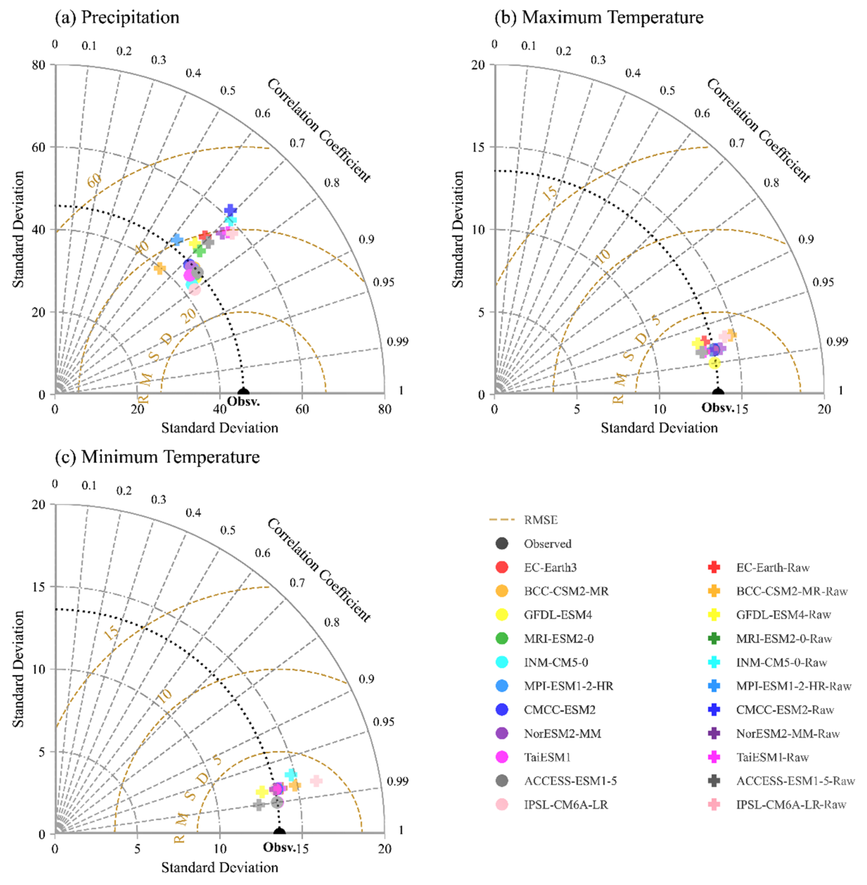
This study evaluated the performance of the monthly climate variables of 11 CMIP6 GCMs at 13 meteorological stations. The results showed that the precipitation of GCMs was obviously overestimated, the maximum temperature was obviously underestimated, and the error of the minimum temperature was relatively small (see Figures S2-1 and S2-2). Additionally, the Delta Change method can effectively correct the overestimation of precipitation and underestimation of the maximum temperature, as well as some minor deviations in the minimum temperature. Figure 2 shows the improvement in bias-corrected GCMs compared to raw GCMs in terms of Taylor diagrams and the Pearson correlation, standard deviation, and RMSE. The results showed that the consistency between climate variables of each GCM and observed values were significantly enhanced after using the Delta Change method. The standard deviation of precipitation from bias-corrected GCMs reduced by up to 29%, the RMSE reduced by 10–31%, and the Pearson correlation improved by 2–19%, compared to that from raw GCMs. Additionally, the standard deviation of maximum and minimum temperatures reduced by up to 8% and 16%, the Root Mean Square Error (RMSE) reduced by 4–32% and 3–35%, and the correlation coefficients increased by 0.1–1.5% and 0.1–0.7%, respectively.
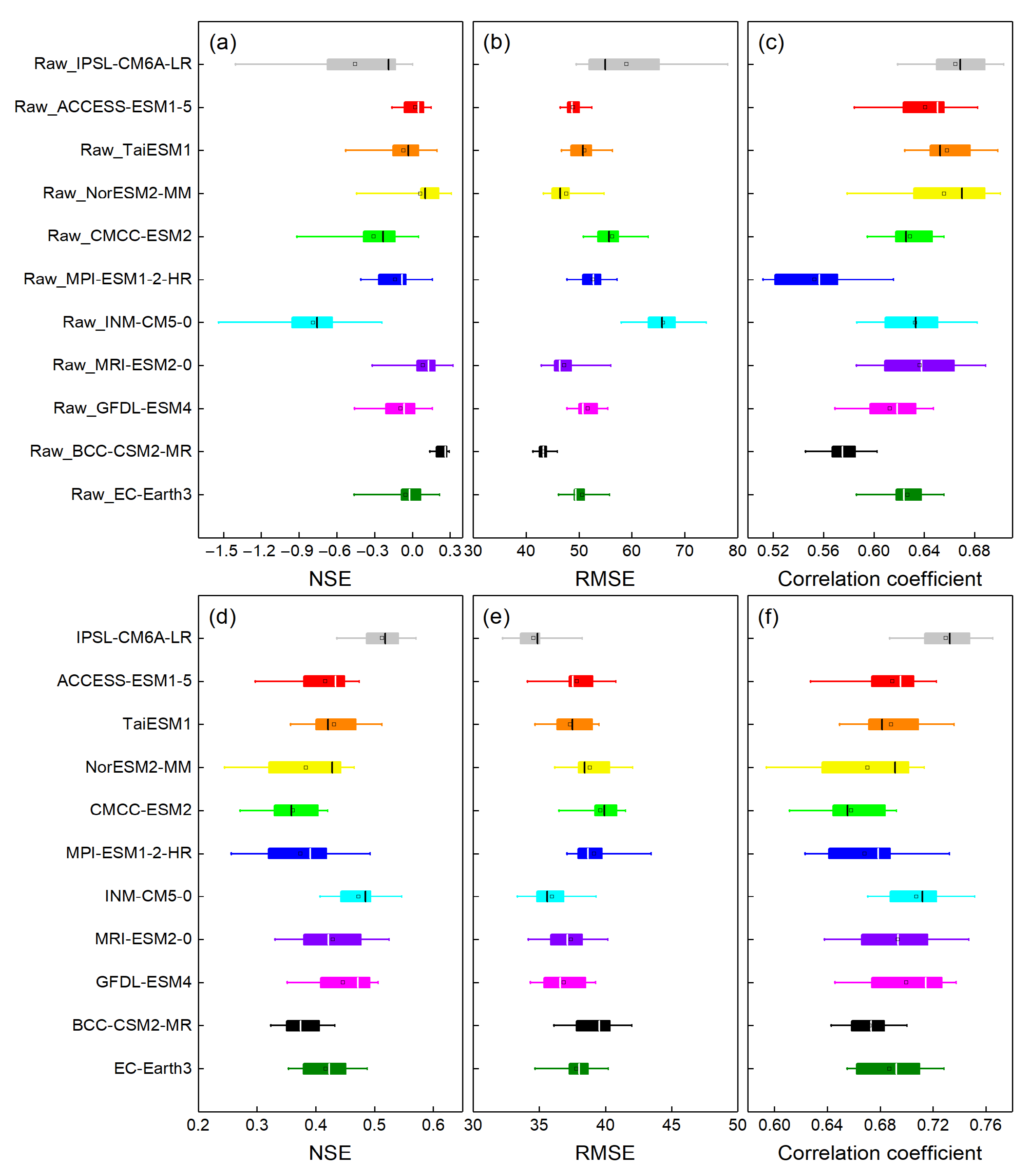
Additionally, the box plots were used to compare the consistency, errors, and correlations of precipitation, maximum temperature, and minimum temperature between 11 GCMs and observed values at 13 meteorological stations before and after Delta Change bias correction (see Figure 3, Figure 4 and Figure 5). As shown in Figure 3a–c, there were relatively low NSE (−1.54 ≤ NSE ≤ 0.32), high RMSE (41 ≤ RMSE ≤ −79 mm), and high correlation coefficient (0.51 ≤ R ≤ 0.70) between the precipitation of raw GCMs and observed values, and significant spatial variability in these metrics across different meteorological stations (0.15 ≤ ΔNSE ≤ 1.41, 4 ≤ ΔRMSE ≤ 29, and 0.06 ≤ ΔR ≤ 0.12). After bias correction, the NSE values significantly increased overall (0.24 ≤ NSE ≤ 0.57), the RMSE values greatly decreased (32 ≤ RMSE ≤ 44 mm), and the correlation coefficients slightly improved (0.51 ≤ R ≤ 0.7; Figure 3d–f). Furthermore, the spatial variability of these metrics across different meteorological stations significantly decreased, particularly for NSE (0.11 ≤ ΔNSE ≤ 0.24) and RMSE (4 ≤ ΔRMSE ≤ 7).
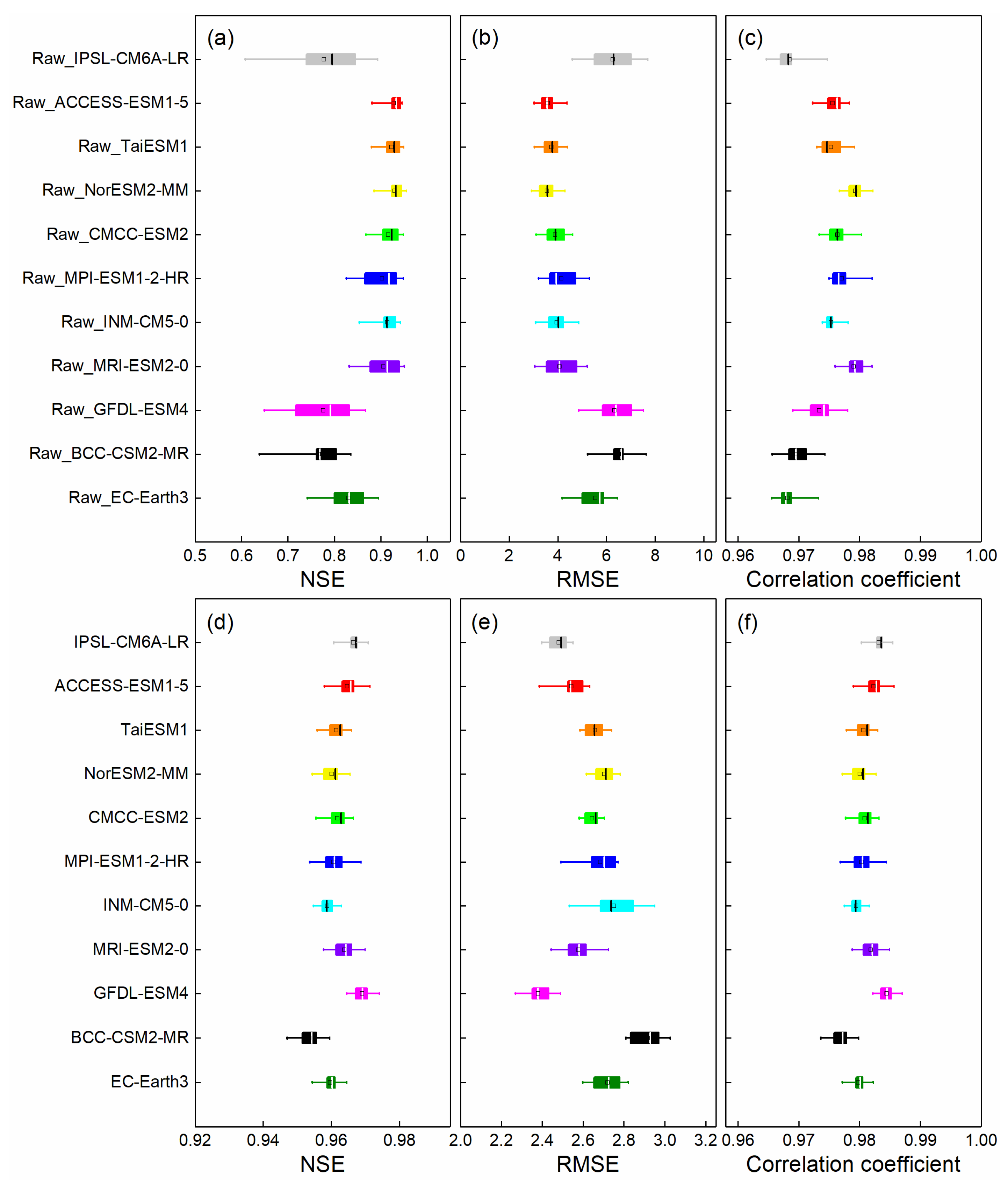
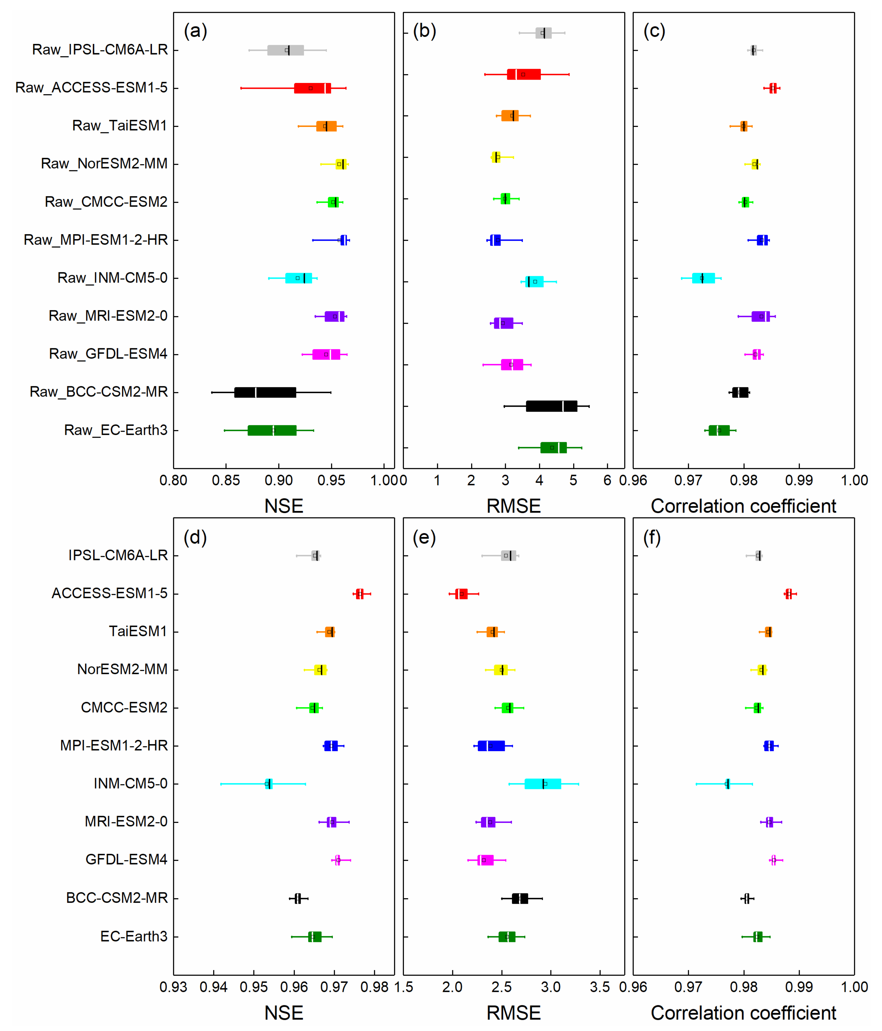
Compared to precipitation, the maximum/minimum temperature from GCMs were relatively consistent with observations. As shown in Figure 4a–c, the maximum temperature from raw-GCMs exhibited higher NSE (0.61 ≤ NSE ≤ 0.96), lower RMSE (2.9 ≤ RMSE ≤ 7.7 °C), and extremely high correlation coefficient (0.96 ≤ R ≤ 0.98), with relatively small spatial variability in these metrics across different stations. After bias correction, the NSE values significantly improved (0.95 ≤ NSE ≤ 0.97), the RMSE values substantially decreased (2.27 ≤ RMSE ≤ 3.03 °C), and the correlation coefficients slightly increased (0.97 ≤ R ≤ 0.99; Figure 4d–f). Additionally, the spatial variability of these metrics across different meteorological stations significantly reduced, particularly for NSE and RMSE. The minimum temperatures also exhibited similar characteristics, as shown in Figure 5.

3.2. Performance Evaluation of Simulated Streamflow in Historical Period

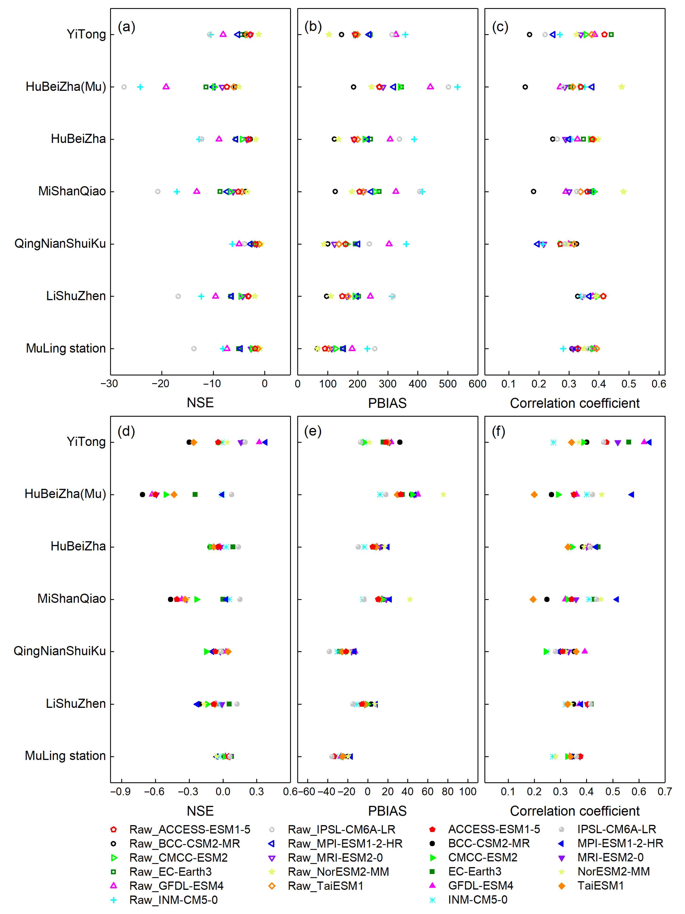
Based on the calibrated SWAT+ (see Supplementary Material S4 for calibration, validation, and evaluation results), we assessed the streamflow simulation performance of SWAT+ driven by raw and bias-corrected GCMs for the period 1961–2014, by utilizing NSE, PBIAS, and correlation coefficient (R). Results showed that the SWAT+ model driven by raw GCMs showed poor performance in simulating streamflow at the seven hydrological stations, with NSE values ranging from −0.69 to −27.32, PBIAS values ranging from 65.4 to 532.10, and correlation coefficients between 0.16 and 0.48. Among these, the QNSK station exhibited the highest overall NSE, followed by YT and ML stations, with HBZm showing the worst simulation results. The mean and range of PBIAS for ML, LSZ, and QNSK were relatively smaller compared to other stations, and their mean R values were relatively higher, with smaller ranges. Therefore, the GCMs selected in this study, before bias correction, could drive the SWAT+ model to perform slightly better in simulating streamflow for ML, LSZ, and QNSK compared to other stations. From the perspective of GCMs, the SWAT+ models driven by NorESM2-MM and TaiESM1 exhibited relatively good streamflow simulation performance for seven hydrological stations, while the models driven by IPSL-CM6A-LR and INM-CM5-0 exhibited poor streamflow simulation performance (Figure 6a–c). After bias correction, the streamflow simulation performance of the SWAT+ model driven by the selected GCMs significantly improved, with NSE values ranging from −0.71 to 0.38, PBIAS values from −38.4 to 75.7, and correlation coefficients from 0.2 to 0.64 (Figure 6d–f). Among these stations, the average NSE at YT station was the highest, but with considerable variability across different GCMs, followed by ML station with small variability. The average PBIAS at LSZ was the smallest, followed by HBZ, and their variability was relatively small across different GCMs. The correlation coefficient at YT station was the largest with considerable variability, followed by HBZ station with relatively small variability. Which indicated that bias-corrected GCMs in this study can drive the SWAT+ model to perform relatively well in simulating streamflow in the Xiaoxingkai Lake Basin, especially at HBZ and YT stations.

3.3. Streamflow Simulation and Prediction Based on Multi-Model Weighted Average Ensemble

To enhance the accuracy of streamflow simulation and prediction results of the SWAT+ model driven by GCMs, this study employed BMA to perform a weighted average ensemble of multi-model-driven streamflow simulations (see Table S5-1 for weights). The results were then compared with those obtained using a simple arithmetic average. According to Figure 7, the simple arithmetic average ensemble results did not accurately reflect the trends of observed streamflow, which was same at the whole basin (see Figure S3-1). In contrast, the streamflow trends derived from BMA showed a higher consistency with both the observed streamflow and the streamflow trends simulated based on meteorological observations, which indicated that the BMA method can effectively enhance the accuracy of streamflow simulation and prediction.
Based on historical simulated inflow of Xiaoxingkai Lake and inflows driven by GCMs, we obtained the weights of the BMA ensemble method. Hence, the multi-model weighted average inflows of Xiaoxingkai Lake under historical and future climate scenarios were obtained, as shown in Figure 8a,b. Additionally, the wavelet decomposition was performed to obtain the interdecadal variation trend of inflow, as shown in Figure 8c,d. During 1961–2014, the inflow of Xiaoxingkai Lake showed a “W”—shaped changing trend, with two low-flow periods occurring in the late 1970s and early 2000s, and a high-flow period occurring around the 1990s. The BMA-integrated inflow can better reflect this trend of change. Under SSP245 and SSP585 scenarios, the inflow of Xiaoxingkai Lake will fluctuate, and the overall trend will not be significant. On the interdecadal scale, the inflow of the Xiaoxingkai lake under the SSP245 scenario will experience three peak flow periods in the mid-2050s, late 2080s, and mid-2090s, but they will not be significant compared to the average level. Under the SSP585 scenario, the inflow of Xiaoxingkai Lake will show two significant high-flow periods in the late 2040s and around 2070s, and that in the 2070s will be particularly evident. Additionally, there will be two distinct periods of low-flow during the 2030s–2040s and in the mid-2090s.
To evaluate near-term and long-term future changes in streamflow entering Xiaoxingkai Lake under SSP245 and SSP585 scenarios, the future period (2020–2100) was divided into two sub-periods: 2020–2060 (2040s) and 2061–2100 (2080s). Figure 9 presents variations in annual, wet season (May–September), normal-flow season (March, April, October, and November), and dry season (December–February) inflows relative to the historical baseline for both scenarios and periods. For annual averages, inflow increased from 57.84 m3/s in the historical period to 66.12 m3/s (+14.3%) under SSP245 and 65.75 m3/s (+13.7%) under SSP585 in the 2040s, much lower than in the 2080s (74.33 m3/s, +28.5% under SSP245; 73.87 m3/s, +27.7% under SSP585; Table S6-1 and Figure 9a). SSP245 consistently yielded slightly higher annual increases than SSP585. Similarly, wet season inflow rose from 95.37 m3/s to 109.77 m3/s (+15.1%) under SSP245 and 109.51 m3/s (+14.8%) under SSP585 in the 2040s, substantially less than in the 2080s (126.55 m3/s, +32.7% under SSP245; 124.90 m3/s, +31.0% under SSP585; Table S6-1 and Figure 9b). For the normal-flow season, inflow increased from 49.81 m3/s to 54.33 m3/s (+9.1%) under SSP245 and 53.02 m3/s (+6.4%) under SSP585 in the 2040s, compared with 56.30 m3/s (+13.0%) and 53.28 m3/s (+7.0%) in the 2080s (Table S6-1 and Figure 9c). Here, the inflow under SSP245 maintained higher increases than SSP585, but the inter-scenario differences widened over time, while differences between sub-periods narrowed within each scenario. In contrast, dry season inflows showed the most dramatic changes. They increased from 5.99 m3/s in the historical period to 9.09 m3/s (+51.7%) under SSP245 and 9.78 m3/s (+63.1%) under SSP585 in the 2040s (Table S6-1 and Figure 9d). By the 2080s, inflows reached 11.34 m3/s (+89.2%) under SSP245 and 16.29 m3/s (+171.7%) under SSP585, indicating that SSP585 produced much stronger streamflow amplification, particularly in the 2080s.

4. Discussion

4.1. Evaluation of GCM Performance and Bias Correction

The accuracy of hydrological projections is fundamentally contingent upon the reliability of climate forcing data [45,46]. Systematic errors inherent in GCMs, coupled with structural discrepancies among them (e.g., parameterizations of cloud microphysics and land-atmosphere interactions), inevitably propagate biases into climate variable projections [21]. These biases are amplified in regions characterized by complex topography or localized convective precipitation regimes, where inter-model variability—particularly in precipitation—becomes pronounced [47,48]. The topography of the Xiaoxingkai Lake Basin is relatively complex, and there are significant differences in climate variables among GCMs, especially in precipitation (see Figure 3). In this study, we selected 11 GCMs from different countries and regions and performed the Delta Change method for bias correction, which reduced the RMSE of precipitation and temperature by 3–35%. During the selection process, we considered only the institutions providing GCMs, data resolution, and usage in previous studies. We further assessed inter-model correlations (taking precipitation as an example, all pairwise R ≤ 0.75) and simulation performance (Taylor skill score > 0.6), which suggested acceptable independence and reliability among the selected GCMs. However, correlation coefficients alone may not fully capture inter-model dependence, and a fixed threshold (e.g., 0.75) should not be considered as a strict indicator of independence [36,49,50]. Identifying the most representative and complementary model subsets, therefore, remains a challenge requiring further research. In addition, the use of the Delta Change method at the monthly scale ensures stability for long-term hydrological assessments but does not fully capture daily scale variability and extremes. Future studies should not only compare different bias correction methods and quantify their uncertainties, but also comprehensively evaluate the impact of uncertainties caused by climate model selection, downscaling, and bias correction methods on watershed streamflow. Establishing more robust criteria for GCM independence (e.g., mutual information [51], cluster analysis [49], or multi-metric ensemble diagnostics [36]) and adopting an optimal bias correction method will be essential to reduce the uncertainty in future streamflow projections.

4.2. Uncertainty of Streamflow Projections

The accuracy of streamflow prediction is constrained not only by the GCMs themselves and data processing methods, but also by changes in underlying surface conditions and socio-economic activities. For example, Chawanda, Nkwasa, Thiery and van Griensven [45] considered not only future climate change but also land use change scenarios when assessing the impact of climate change on future water resources of Africa. It was not considered in this study, which may affect the accuracy of streamflow predictions.
In this study, the BMA method was used to optimize ensemble streamflow predictions and mitigate uncertainty. The BMA weights estimated from the historical period were directly applied to future scenarios, which is a common practice in ensemble climate–hydrology assessments. However, previous studies have pointed out that model skill may not remain stationary under future climate conditions [52,53]. This non-stationarity suggests that the relative performance of GCMs could shift in future projections, implying that the direct application of historically derived weights may introduce additional uncertainty into the ensemble projections. Consequently, while the current approach ensures methodological consistency, it may underestimate the variability of future ensemble behavior. Future work should therefore consider time-varying or scenario-dependent weighting schemes, or hybrid ensemble approaches, to enhance the robustness of hydrological projections under changing climate conditions.
Additionally, the performance of BMA is highly sensitive to the continuity and representativeness of observational data. Discontinuities in the collected hydrological monitoring data led to anomalies in the BMA weighted ensemble results during data-gap periods. To mitigate these anomalies, this study derived an alternative set of weights based on historical streamflow simulations driven by observed meteorological data. These weights were applied to correct the GCM-based streamflow projections through secondary weighted averaging. While this approach effectively reduced outliers in streamflow predictions, the associated uncertainties remain challenging to quantify. Future research should explore the integration of data assimilation techniques and machine learning methods with BMA to improve streamflow projection accuracy. In addition, tests excluding stations with short (MSQ, HBZm, and YT) or incomplete observation records (HBZm and YT) showed only minor improvements in NSE (0.023 and 0.007, respectively), suggesting limited impact on overall results. In similar studies across other basins, the potential effects of calibration duration and severe gaps in observation data on runoff simulation and prediction should be further evaluated. Where conditions permit, stations with extensive missing records should be excluded, and simulations should be conducted over unified periods with continuous observations.

4.3. Future Streamflow Changes and Potential Mechanisms of Xiaoxingkai Lake

The prediction results of this study showed that although streamflow in the Xiaoxingkai Lake Basin was projected to increase under both SSP245 and SSP585 scenarios, a particularly notable finding was that under the SSP585 scenario, the increase in dry season streamflow in both the 2040s (+63.1%) and the 2080s (+171.7%) would be significantly higher than those under SSP245 scenario (+51.7% in the 2040s and +89.2% in the 2080s), compared to the historical baseline. This phenomenon might be because that under the uncontrolled high-emission scenario (SSP585), significantly warmer dry season temperatures would lead to more liquid precipitation, thereby promoting increased streamflow. Similar results have been reported in other regions. For instance, Fuso et al. [54] demonstrated that in a high-altitude basin in Northern Italy, rising winter temperatures will increase liquid precipitation at the expense of solid precipitation, consequently increasing streamflow. The climatic characteristics of the Xiaoxingkai Lake Basin, located in a temperate continental monsoon zone, keep the entire dry season in a frozen state under current conditions. However, intensified warming under SSP585 could accelerate snowmelt processes, leading to earlier snowmelt may contribute to higher baseflow in the dry season. Overall, these results suggest that enhanced dry season runoff under SSP585 reflects the combined effects of more liquid precipitation and earlier snowmelt-induced baseflow. This highlights the potential hydrological consequences of uncontrolled warming and underscores the importance of controlling CO2 emissions for mitigating the impacts of climate change on the basin’s hydrological cycle. Future research should employ techniques such as baseflow partitioning to quantitatively disentangle the relative contributions of precipitation phase shifts and snowmelt processes to the projected dry season streamflow changes under different emission scenarios.

4.4. Implications for Transboundary Water Resource Management

As a transboundary watershed shared by China and Russia, the Xiaoxingkai Lake Basin is highly sensitive to climate-driven hydrological changes. Our findings of amplified seasonal runoff variability underscore critical implications for cooperative management. First, altered seasonal regimes may affect water availability and influence bilateral water rights allocation arrangements. For example, although an increase in runoff during low-flow periods may provide more available water resources, differences in socio-economic development have led to divergent perspectives between China and Russia regarding water allocation. Moreover, increased runoff during the rainy season is likely to substantially elevate flood risks, requiring that water allocation and management be closely integrated with flood-control operations. Adaptive allocation mechanisms that integrate hydrological forecasts and explicitly account for uncertainty are therefore necessary to mitigate potential disputes. Second, changes in inflow dynamics threaten the ecological stability of the Xingkai Lake wetlands, a Ramsar-listed site of international significance. Modified inundation patterns may disrupt biodiversity and ecosystem services. Coordinated measures—such as maintaining minimum ecological flows and establishing early-warning systems for droughts and floods—are essential for sustaining ecological resilience. Finally, experiences from other international basins demonstrate that joint monitoring, data sharing, and cooperative governance can reduce transboundary tensions [55,56]. Establishing a bilateral mechanism for climate and hydrological information exchange would enhance adaptive capacity and strengthen basin-wide resilience to future climate uncertainties. Overall, linking scientific projections with policy-level coordination is vital. By integrating climate-informed hydrological modeling with cooperative governance, China and Russia can safeguard ecological and socio-economic sustainability while enhancing long-term water security in this strategically important basin.

5. Conclusions

This study employed daily precipitation, maximum temperature, and minimum temperature projections from 11 CMIP6 GCMs under the SSP245 and SSP585 scenarios to drive the SWAT+ model, predicting streamflow dynamics in the Xiaoxingkai Lake Basin during 2021–2060 (2040s) and 2061–2100 (2080s). The Delta Change method was used to correct GCM biases, and the BMA method was applied to integrate multi-model streamflow predictions. The research results indicated that the Delta Change method effectively mitigated GCM biases, thereby improving precipitation, temperature, and subsequent SWAT+ streamflow simulations; the weighted average ensemble method of BMA outperformed simple arithmetic averaging in multi-model streamflow ensemble, providing more robust projections by reducing the influence of inter-model uncertainty; streamflow entering Xiaoxingkai Lake was amplified in all seasons from the 2040s to 2080s, with the most pronounced increases in the dry season (the percentage change relative to the historical baseline increased from 51.7% to 89.2% under SSP245 and from 63.1% to 171.7% under SSP585). SSP245 consistently yielded higher streamflow gains than SSP585 in annual, wet-, and normal-flow seasons (e.g., wet season: +32.7% vs. +31.0% in the 2080s), whereas SSP585 produced disproportionately larger dry season surges, exceeding SSP245 by 82.5% in the 2080s.
By integrating SWAT+ with CMIP6 scenarios, this study provides critical insights into climate-driven hydrological changes in the Xiaoxingkai Lake Basin. As a transboundary watershed shared between China and Russia, the basin represents a unique and underexplored case for assessing climate change impacts on hydrological processes, highlighting its international significance and ecological significance. Methodologically, the study demonstrates the advantage of BMA in optimizing ensemble predictions and mitigating model uncertainty, offering an innovative contribution to hydrological impact assessments. By quantifying potential hydrological shifts under climate warming scenarios, this study contributes to a deeper understanding of hydrological sustainability and the resilience of hydrological processes and wetland ecosystems in transboundary lake basins.

Supplementary Materials

The following supporting information can be downloaded at: https://www.mdpi.com/article/10.3390/su17177901/s1, Table S1-1: Correlation matrix of historical monthly precipitation among 11 CMIP6 GCMs in the Xiaoxingkai Lake Basin; Figure S2-1: Seasonal variations in observed and simulated precipitation at different meteorological stations during historical period; Figure S2-2: Simulation and prediction results of precipitation, maximum temperature, and minimum temperature during historical and future periods; Figure S3-1. Simulation and prediction results of precipitation, maximum temperature, and minimum temperature during historical and future periods; Table S4-1: Parameters related to streamflow in SWAT+ model with the land use data in 2010; Figure S4-1: Sensitivity of 23 model parameters. Panels (a–g) refer to parameters sensitivity at MuLing, LiShuZhen, QingNianShuiKu, MiShanQiao, HuBeiZha, HuBeiZha (Mu), and YiTong stations, respectively; Figure S4-2: Observed and simulated monthly streamflow based on SWAT+ with the static land use/land cover in 2010. (a) The monthly precipitation in Xiaoxingkai Lake Basin from 1961 to 2017. (a1, a2) The average monthly precipitation during calibration (1961–1987) and validation periods (2002–2017). (b–g) The monthly streamflow at the seven hydrological stations. (b1–g1, b2–g2) The average monthly streamflow during calibration and validation periods, respectively; Table S4-2: Evaluation of monthly streamflow simulation results based on SWAT+ with static land use/land cover in 2010 in the Xiaoxingkai Lake Basin; Table S5-1: Weights from Bayesian Model Averaging of streamflow simulations based on 11 bias-corrected CMIP6 GCMs; Table S6-1: Projected changes in seasonal and annual average streamflow under SSP245 and SSP585 relative to the historical baseline (1961–2014).

Author Contributions

Conceptualization, X.W. and C.F.; methodology, F.X. and X.W.; data curation, F.X.; formal analysis, F.X.; investigation, F.X.; resources, P.W., X.W. and C.F.; writing—original draft preparation, F.X., Y.W. and J.Z.; writing—review and editing, F.X., Y.W. and P.W.; visualization, F.X.; Supervision, X.W. and C.F.; project Administration, P.W., X.W. and C.F.; funding Acquisition, P.W., X.W. and F.X. All authors have read and agreed to the published version of the manuscript.

Funding

This research was funded by the National Key Research and Development Program of China—Science & Technology Cooperation Project of Chinese and Russian Government “Sustainable Transboundary Nature Management and Green Development Modes in the Context of Emerging Economic Corridors and Biodiversity Conservation Priorities in the South of the Russian Far East and Northeast China (grant number 2023YFE0111300)”; the National Key Research and Development Program of China [grant number 2019YFA0607102]; the Natural Science Basic Research Program in Shaanxi Province [grant number 2025JC–YBQN–338]; the Doctoral Talent Introduction and Research Initiation Program of Shaanxi University of Technology [grant number SLGRCQD027].

Institutional Review Board Statement

Not applicable.

Informed Consent Statement

Not applicable.

Data Availability Statement

The original contributions presented in this study are included in the article. Further inquiries can be directed to the corresponding author.

Conflicts of Interest

The authors declare no conflicts of interest.

References

  1. IPCC. The refinement to the 2006 IPCC guidelines for national greenhouse gas inventories. Fundam. Appl. Climatol. 2019, 2, 5–13. [Google Scholar] [CrossRef]
  2. IPCC. Climate Change 2021—The Physical Science Basis: Working Group I Contribution to the Sixth Assessment Report of the Intergovernmental Panel on Climate Change; Cambridge University Press: Cambridge, UK, 2023. [Google Scholar]
  3. Yang, D.; Yang, Y.; Xia, J. Hydrological cycle and water resources in a changing world: A review. Geogr. Sustain. 2021, 2, 115–122. [Google Scholar] [CrossRef]
  4. Labat, D.; Ronchail, J.; Callede, J.; Guyot, J.L.; De Oliveira, E.; Guimaraes, W. Wavelet analysis of Amazon hydrological regime variability. Geophys. Res. Lett. 2004, 31, L02501. [Google Scholar] [CrossRef]
  5. Li, W.; Liu, H.; Gao, P.; Yang, A.; Fei, Y.; Wen, Y.; Su, Y.; Yuan, X. Development of an MPE-BMA Ensemble Model for Runoff Prediction Under Future Climate Change Scenarios: A Case Study of the Xiangxi River Basin. Sustainability 2025, 17, 4714. [Google Scholar] [CrossRef]
  6. Faramarzi, M.; Abbaspour, K.C.; Vaghefi, S.A.; Farzaneh, M.R.; Zehnder, A.J.B.; Srinivasan, R.; Yang, H. Modeling impacts of climate change on freshwater availability in Africa. J. Hydrol. 2013, 480, 85–101. [Google Scholar] [CrossRef]
  7. Zhao, Z.X.; Huo, A.D.; Liu, Q.; Yang, L.Y.; Luo, C.X.; Ahmed, A.; Elbeltagi, A. Assessment of urban inundation and prediction of combined flood disaster in the middle reaches of Yellow river basin under extreme precipitation. J. Hydrol. 2024, 640, 131707. [Google Scholar] [CrossRef]
  8. Legesse, T.G.; Dong, G.; Dong, X.B.; Qu, L.P.; Chen, B.R.; Daba, N.A.; Sorecha, E.M.; Zhu, W.; Lei, T.A.J.; Shao, C.L. The extreme wet and large precipitation size increase carbon uptake in Eurasian meadow steppes: Evidence from natural and manipulated precipitation experiments. Environ. Res. 2023, 237, 117029. [Google Scholar] [CrossRef] [PubMed]
  9. Gulahmadov, N.; Chen, Y.N.; Gulakhmadov, A.; Rakhimova, M.; Gulakhmadov, M. Quantifying the Relative Contribution of Climate Change and Anthropogenic Activities on Runoff Variations in the Central Part of Tajikistan in Central Asia. Land 2021, 10, 525. [Google Scholar] [CrossRef]
  10. Yang, Z.L.; Bai, P. Response of runoff and its components to climate change in the Manas River of the Tian Shan Mountains. Adv. Clim. Change Res. 2024, 15, 62–74. [Google Scholar] [CrossRef]
  11. Gray, L.C.; Zhao, L.; Stillwell, A.S. Impacts of climate change on global total and urban runoff. J. Hydrol. 2023, 620, 129352. [Google Scholar] [CrossRef]
  12. Burns, G.Z.; Fowler, K.J.A.; Horne, A.C. Stress testing climate change impacts on snow cover and streamflow in southeast Australia. J. Hydrol. 2024, 644, 132031. [Google Scholar] [CrossRef]
  13. Deng, C.; Yin, X.; Zou, J.C.; Wang, M.M.; Hou, Y.K. Assessment of the impact of climate change on streamflow of Ganjiang River catchment via LSTM-based models. J. Hydrol.-Reg. Stud. 2024, 52, 101716. [Google Scholar] [CrossRef]
  14. Tan, L.; Feng, P.; Li, B.; Huang, F.; Liu, D.L.; Ren, P.; Liu, H.; Srinivasan, R.; Chen, Y. Climate change impacts on crop water productivity and net groundwater use under a double-cropping system with intensive irrigation in the Haihe River Basin, China. Agric. Water Manag. 2022, 266, 107560. [Google Scholar] [CrossRef]
  15. Hamed, M.M.; Nashwan, M.S.; Shahid, S.; bin Ismail, T.; Wang, X.J.; Dewan, A.; Asaduzzaman, M. Inconsistency in historical simulations and future projections of temperature and rainfall: A comparison of CMIP5 and CMIP6 models over Southeast Asia. Atmos. Res. 2022, 265, 105927. [Google Scholar] [CrossRef]
  16. Song, Y.H.; Nashwan, M.S.; Chung, E.S.; Shahid, S. Advances in CMIP6 INM-CM5 over CMIP5 INM-CM4 for precipitation simulation in South Korea. Atmos. Res. 2021, 247, 105261. [Google Scholar] [CrossRef]
  17. Jiang, D.; Hu, D.; Tian, Z.; Lang, X. Differences between CMIP6 and CMIP5 Models in Simulating Climate over China and the East Asian Monsoon. Adv. Atmos. Sci. 2020, 37, 1102–1118. [Google Scholar] [CrossRef]
  18. Try, S.; Tanaka, S.; Tanaka, K.; Sayama, T.; Khujanazarov, T.; Oeurng, C. Comparison of CMIP5 and CMIP6 GCM performance for flood projections in the Mekong River Basin. J. Hydrol. Reg. Stud. 2022, 40, 101035. [Google Scholar] [CrossRef]
  19. Wang, Y.; Li, H.; Wang, H.; Sun, B.; Chen, H. Evaluation of CMIP6 model simulations of extreme precipitation in China and comparison with CMIP5. Acta Meteorol. Sin. 2021, 79, 369–386. [Google Scholar]
  20. O’Neill, B.C.; Tebaldi, C.; van Vuuren, D.P.; Eyring, V.; Friedlingstein, P.; Hurtt, G.; Knutti, R.; Kriegler, E.; Lamarque, J.-F.; Lowe, J.; et al. The Scenario Model Intercomparison Project (ScenarioMIP) for CMIP6. Geosci. Model Dev. 2016, 9, 3461–3482. [Google Scholar] [CrossRef]
  21. Eyring, V.; Bony, S.; Meehl, G.A.; Senior, C.A.; Stevens, B.; Stouffer, R.J.; Taylor, K.E. Overview of the Coupled Model Intercomparison Project Phase 6 (CMIP6) experimental design and organization. Geosci. Model Dev. 2016, 9, 1937–1958. [Google Scholar] [CrossRef]
  22. Chen, C.; Gan, R.; Feng, D.; Yang, F.; Zuo, Q. Quantifying the contribution of SWAT modeling and CMIP6 inputting to streamflow prediction uncertainty under climate change. J. Clean. Prod. 2022, 364, 132675. [Google Scholar] [CrossRef]
  23. Zhang, L.; Chen, X.; Xin, X. Short commentary on CMIP6 Scenario Model Intercomparison Project (ScenarioMIP). Clim. Change Res. 2019, 15, 519–525. [Google Scholar] [CrossRef]
  24. Zhou, J.; Lu, H.; Yang, K.; Jiang, R.; Yang, Y.; Wang, W.; Zhang, X. Projection of China’s future runoff based on the CMIP6 mid-high warming scenarios. Sci. China Earth Sci. 2023, 66, 528–546. [Google Scholar] [CrossRef]
  25. Jian, S.; Pei, Y.; Zhu, T.; Yu, X. Spatiotemporal change and attribution analysis of future runoff on the Yellow River basin of China. J. Hydrol. Reg. Stud. 2023, 49, 101494. [Google Scholar] [CrossRef]
  26. Song, Y.H.; Chung, E.S.; Shahid, S. Differences in extremes and uncertainties in future runoff simulations using SWAT and LSTM for SSP scenarios. Sci. Total Environ. 2022, 838, 156162. [Google Scholar] [CrossRef]
  27. Zhu, L.J.; Zhou, H.X.; Xie, X.Y.; Li, X.K.; Zhang, D.Y.; Jia, L.M.; Wei, Q.B.; Zhao, Y.; Wei, Z.M.; Ma, Y.Y. Effects of floodgates operation on nitrogen transformation in a lake based on structural equation modeling analysis. Sci. Total Environ. 2018, 631–632, 1311–1320. [Google Scholar] [CrossRef]
  28. Yuan, Y.X.; Jiang, M.; Liu, X.T.; Yu, H.X.; Otte, M.L.; Ma, C.X.; Her, Y.G. Environmental variables influencing phytoplankton communities in hydrologically connected aquatic habitats in the Lake Xingkai basin. Ecol. Indic. 2018, 91, 1–12. [Google Scholar] [CrossRef]
  29. Xiao, F.Y.; Wang, X.M.; Fu, C.S. Impacts of land use/land cover and climate change on hydrological cycle in the Xiaoxingkai Lake Basin. J. Hydrol.-Reg. Stud. 2023, 47, 101422. [Google Scholar] [CrossRef]
  30. Song, K.; Wang, Z.; Li, L.; Tedesco, L.; Li, F.; Jin, C.; Du, J. Wetlands shrinkage, fragmentation and their links to agriculture in the Muleng–Xingkai Plain, China. J. Environ. Manag. 2012, 111, 120–132. [Google Scholar] [CrossRef] [PubMed]
  31. Crosbie, R.S.; Dawes, W.R.; Charles, S.P.; Mpelasoka, F.S.; Summerell, G.K. Differences in future recharge estimates due to GCMs, downscaling methods and hydrological models. Geophys. Res. Lett. 2011, 38, L11406. [Google Scholar] [CrossRef]
  32. Xiao, D.; Liu, D.L.; Wang, B.; Feng, P.; Tang, J. Climate change impact on yields and water use of wheat and maize in the North China Plain under future climate change scenarios. Agric. Water Manag. 2020, 238, 1–15. [Google Scholar] [CrossRef]
  33. Asseng, S.; Martre, P.; Maiorano, A.; Rötter, R.P.; Ewert, F. Climate change impact and adaptation for wheat protein. Glob. Change Biol. 2018, 25, 155–173. [Google Scholar] [CrossRef]
  34. Thomson, A.M.; Brown, R.A.; Rosenberg, N.J.; Srinivasan, R.; Izaurralde, R.C. Climate Change Impacts for the Conterminous USA: An Integrated Assessment Part 4: Water Resources. Clim. Change 2005, 69, 43–65. [Google Scholar] [CrossRef]
  35. Najafi, M.R.; Moradkhani, H.; Jung, I.W. Assessing the uncertainties of hydrologic model selection in climate change impact studies. Hydrol. Process. 2011, 25, 2814–2826. [Google Scholar] [CrossRef]
  36. Ashfaq, M.; Rastogi, D.; Kitson, J.; Abid, M.A.; Kao, S.C. Evaluation of CMIP6 GCMs Over the CONUS for Downscaling Studies. J. Geophys. Res. Atmos. 2022, 127, e2022JD036659. [Google Scholar] [CrossRef]
  37. Li, Z.-L.; Jiao, X.-Z. Evaluation and projections of summer daily precipitation over Northeastern China in an optimal CMIP6 Multimodel Ensemble. Clim. Dyn. 2024, 62, 6235–6251. [Google Scholar] [CrossRef]
  38. Li, C.; Fang, H. Assessment of climate change impacts on the streamflow for the Mun River in the Mekong Basin, Southeast Asia: Using SWAT model. Catena 2021, 201, 105199. [Google Scholar] [CrossRef]
  39. Buhay Bucton, B.G.; Shrestha, S.; Kc, S.; Mohanasundaram, S.; Virdis, S.G.P.; Chaowiwat, W. Impacts of climate and land use change on groundwater recharge under shared socioeconomic pathways: A case of Siem Reap, Cambodia. Environ. Res. 2022, 211, 113070. [Google Scholar] [CrossRef]
  40. Tan, M.L.; Liang, J.; Samat, N.; Chan, N.W.; Haywood, J.M.; Hodges, K. Hydrological Extremes and Responses to Climate Change in the Kelantan River Basin, Malaysia, Based on the CMIP6 HighResMIP Experiments. Water 2021, 13, 1472. [Google Scholar] [CrossRef]
  41. Maraun, D. Bias Correcting Climate Change Simulations—A Critical Review. Curr. Clim. Change Rep. 2016, 2, 211–220. [Google Scholar] [CrossRef]
  42. Shrestha, M.; Acharya, S.C.; Shrestha, P.K. Bias correction of climate models for hydrological modelling-are simple methods still useful? Meteorol. Appl. 2017, 24, 531–539. [Google Scholar] [CrossRef]
  43. Konapala, G.; Mishra, A.K.; Wada, Y.; Mann, M.E. Climate change will affect global water availability through compounding changes in seasonal precipitation and evaporation. Nat. Commun. 2020, 11, 3044. [Google Scholar] [CrossRef]
  44. Bieger, K.; Arnold, J.G.; Rathjens, H.; White, M.J.; Bosch, D.D.; Allen, P.M.; Volk, M.; Srinivasan, R. Introduction to SWAT+, A Completely Restructured Version of the Soil and Water Assessment Tool. JAWRA J. Am. Water Resour. Assoc. 2017, 53, 115–130. [Google Scholar] [CrossRef]
  45. Chawanda, C.J.; Nkwasa, A.; Thiery, W.; van Griensven, A. Combined impacts of climate and land-use change on future water resources in Africa. Hydrol. Earth Syst. Sci. 2024, 28, 117–138. [Google Scholar] [CrossRef]
  46. Mankin, K.R.; Mehan, S.; Green, T.R.; Barnard, D.M. Review of gridded climate products and their use in hydrological analyses reveals overlaps, gaps, and the need for a more objective approach to selecting model forcing datasets. Hydrol. Earth Syst. Sci. 2025, 29, 85–108. [Google Scholar] [CrossRef]
  47. Carmichael, M.J.; Lunt, D.J.; Huber, M.; Heinemann, M.; Kiehl, J.; LeGrande, A.; Loptson, C.A.; Roberts, C.D.; Sagoo, N.; Shields, C.; et al. A model–model and data–model comparison for the early Eocene hydrological cycle. Clim. Past 2016, 12, 455–481. [Google Scholar] [CrossRef]
  48. Eghdamirad, S.; Johnson, F.; Sharma, A. How reliable are GCM simulations for different atmospheric variables? Clim. Change 2017, 145, 237–248. [Google Scholar] [CrossRef]
  49. Brunner, L.; Pendergrass, A.G.; Lehner, F.; Merrifield, A.L.; Lorenz, R.; Knutti, R. Reduced global warming from CMIP6 projections when weighting models by performance and independence. Earth Syst. Dyn. 2020, 11, 995–1012. [Google Scholar] [CrossRef]
  50. Nguyen, P.L.; Alexander, L.V.; Thatcher, M.J.; Truong, S.C.H.; Isphording, R.N.; McGregor, J.L. Selecting CMIP6 global climate models (GCMs) for Coordinated Regional Climate Downscaling Experiment (CORDEX) dynamical downscaling over Southeast Asia using a standardised benchmarking framework. Geosci. Model Dev. 2024, 17, 7285–7315. [Google Scholar] [CrossRef]
  51. Majhi, A.; Dhanya, C.T.; Chakma, S. Mutual information based weighted variance approach for uncertainty quantification of climate projections. MethodsX 2023, 10, 102063. [Google Scholar] [CrossRef] [PubMed]
  52. Sanderson, B.M.; Wehner, M.; Knutti, R. Skill and independence weighting for multi-model assessments. Geosci. Model Dev. 2017, 10, 2379–2395. [Google Scholar] [CrossRef]
  53. Wang, H.-M.; Chen, J.; Xu, C.-Y.; Chen, H.; Guo, S.; Xie, P.; Li, X. Does the weighting of climate simulations result in a better quantification of hydrological impacts? Hydrol. Earth Syst. Sci. 2019, 23, 4033–4050. [Google Scholar] [CrossRef]
  54. Fuso, F.; Stucchi, L.; Bonacina, L.; Fornaroli, R.; Bocchiola, D. Evaluation of water temperature under changing climate and its effect on river habitat in a regulated Alpine catchment. J. Hydrol. 2023, 616, 128816. [Google Scholar] [CrossRef]
  55. Gao, J.; Castelletti, A.; Burlado, P.; Wang, H.; Zhao, J. Soft-cooperation via data sharing eases transboundary conflicts in the Lancang-Mekong River Basin. J. Hydrol. 2022, 606, 127464. [Google Scholar] [CrossRef]
  56. Zhao, Y.; Zhao, T.; Xiong, X.; Sun, Y. Understanding the conflict and cooperation in the Yarlung Tsangpo-Brahmaputra River Basin under climate change: A quantitative view based on water events. J. Water Clim. Change 2023, 14, 1226–1246. [Google Scholar] [CrossRef]
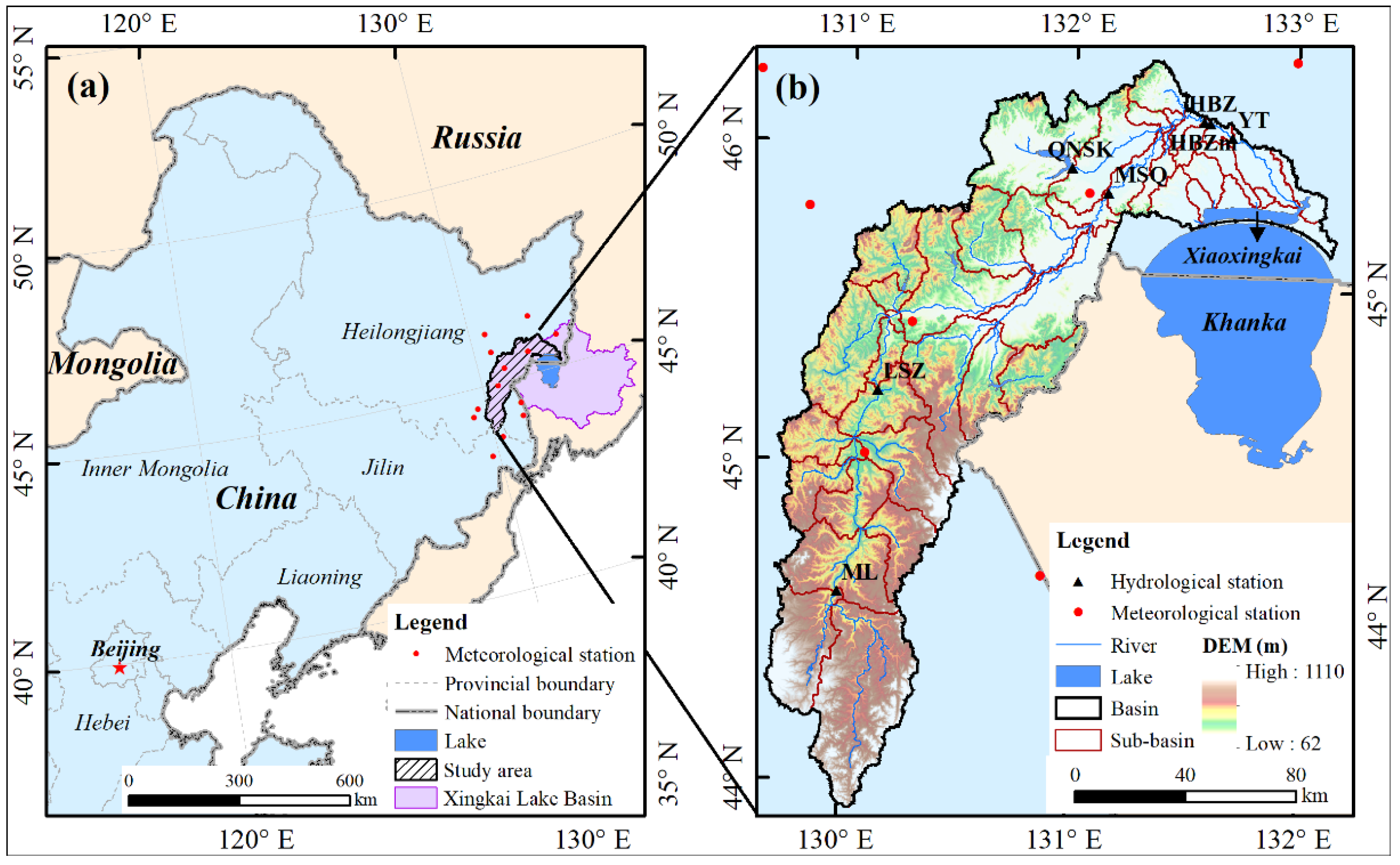
Figure 1. Location of the Xiaoxingkai Lake Basin. (a) Geographic location of the basin within Northeast China; (b) Detailed map of the basin. ML, LSZ, QNSK, MSQ, HBZ, HBZm, and YT in panel (b) refer to hydrological stations of MuLing, LiShuZhen, QingNianShuiKu, MiShanQiao, HuBeiZha, HuBeiZha (Mu), and YiTong, respectively.
Sustainability 17 07901 g001
Figure 2. Comparison between the raw/bias-corrected historical climate variables of 11 CMIP6 GCMs and observations at 13 stations using a Taylor diagram.
Sustainability 17 07901 g002
Figure 3. Box diagram of comparison between the raw and bias-corrected historical precipitation of 11 CMIP6 GCMs and observations at 13 stations. (a) Nash-Sutcliffe efficiency (NSE) before bias correction; (b) Root Mean Square Error (RMSE) before bias correction; (c) Correlation coefficient before bias correction; (d) NSE after bias correction; (e) RMSE after bias correction; (f) Correlation coefficient after bias correction.
Sustainability 17 07901 g003
Figure 4. Box diagram of comparison between the raw and bias-corrected historical maximum temperature of 11 CMIP6 GCMs and observations at 13 stations. (a) Nash-Sutcliffe efficiency (NSE) before bias correction; (b) Root Mean Square Error (RMSE) before bias correction; (c) Correlation coefficient before bias correction; (d) NSE after bias correction; (e) RMSE after bias correction; (f) Correlation coefficient after bias correction.
Sustainability 17 07901 g004
Figure 5. Box diagram of comparison between the raw and bias-corrected historical minimum temperature of 11 CMIP6 GCMs and observations at 13 stations. (a) Nash-Sutcliffe efficiency (NSE) before bias correction; (b) Root Mean Square Error (RMSE) before bias correction; (c) Correlation coefficient before bias correction; (d) NSE after bias correction; (e) RMSE after bias correction; (f) Correlation coefficient after bias correction.
Sustainability 17 07901 g005
Figure 6. Comparison between the streamflow based on raw and bias-corrected historical climate variables of 11 CMIP6 GCMs. (a) Nash-Sutcliffe efficiency (NSE) before bias correction; (b) Percent bias (PBIAS) before bias correction; (c) Correlation coefficient before bias correction; (d) NSE after bias correction; (e) PBIAS after bias correction; (f) Correlation coefficient after bias correction.
Sustainability 17 07901 g006
Figure 7. Comparison among ensemble streamflow simulations, observed streamflow, and streamflow based on observed climate variables (QObs: observed streamflow; QCMA: simulated streamflow based on observed climate data; QGCM.BMA: Bayesian Model Average integrated streamflow from GCM-driven simulations; QGCM.Average: simple arithmetic average integrated from GCM-driven simulations. The shaded area represents the 90% percentile range (P5–P95) of streamflow simulation results, indicating that 90% of the simulated values fall within this interval).
Sustainability 17 07901 g007
Figure 8. Changes in integrated historical and future predictions of streamflow entering Xiaoxingkai Lake based on the Bayesian Weighted Average (BMA) method. (a) Historical streamflow simulations; (b) Wavelet analysis of historical streamflow simulations; (c) Streamflow projections under SSP245 and SSP585 scenarios; (d) Wavelet analysis of streamflow predictions. (QCMA represents historical simulated streamflow based on observed climate data. QGCM.BMA represents BMA-integrated streamflow from GCM-driven simulations. QSSP245 and QSSP585 represent the streamflow prediction results driven by GCM climate variables under the SSP245 and SSP585 scenarios, respectively, while QSSP245.BMA and QSSP585.BMA represent their BMA-integrated results, respectively. The shaded area represents the 90% percentile range (P5–P95) of streamflow simulation results, indicating that 90% of the simulated values fall within this interval).
Sustainability 17 07901 g008
Figure 9. Predicted streamflow variations relative to the historical baseline for annual, wet season, normal-flow season, and dry season under SSP245 and SSP585 scenarios in the 2040s and 2080s. The historical baseline: 1961–2014; Wet season: May–September; Dry season: December–February.
Sustainability 17 07901 g009
Table 1. Information table of selected global climate models.
IDModel NameInstitute IDCountryResolutionTaylor Skill Score
1ACCESS-ESM1-5BoMAustralia250 km0.72
2BCC-CSM2-MRBCCChina100 km0.66
3CMCC-ESM2CMCCItaly100 km0.66
4EC-Earth3EC-EARTHEuropean Union100 km0.70
5GFDL-ESM4NOAA GFDLAmerica100 km0.70
6INM-CM5-0INMRussia100 km0.68
7IPSL-CM6A-LRIPSLFrance250 km0.71
8MPI-ESM1-2-HRMPI-MGermany100 km0.65
9MRI-ESM2-0MRIJapan100 km0.72
10NorESM-MMNCCNorway100 km0.71
11TaiESM1AS-RCECTaiwan, China100 km0.71
Note: (1) This study utilized CMIP6 data archived in the Earth System Grid Federation system. Per the Coupled Model Intercomparison Project’s data governance, all datasets are guaranteed persistent availability through globally distributed nodes. The initial download portal was the LLNL node (https://esgf-node.llnl.gov); the current active access portals include the IPSL node (https://esgf-node.ipsl.upmc.fr/projects/cmip6-ipsl/) and the DKRZ node (https://esgf-data.dkrz.de/projects/cmip6-dkrz/). All links verified on 18 August 2025. (2) Taylor Skill Scores were calculated based on the standard deviation of monthly precipitation from GCMs (δm) and observations (δo), and the correlation coefficient (R) between them. The formula is as: TSS = 4·(1 + R)2/[(δm/δo + δo/δm)2(1 + R0)2], where R0 is set to 1, which is substituted into the formula as the maximum correlation coefficient among all models. A larger TSS indicates a relatively better performance of the GCM.
Table 2. Information table of hydrological stations.
Hydrological StationsAvailable Data RangeMonthly StreamflowAverage Yearly Streamflow
AverageMaximum (Year-Month)
1MuLing1962–1987, 2002–201711.49149.00 (1965-08)11.55
2Lishuzhen1963–1987, 2002–201724.81324.00 (1965-08)24.94
3QingNianShuiKu1961–1987, 2002–20173.1279.80 (1981-08)3.14
4MiShanQiao1979–1987, 2002–201736.69320.00 (2002-08)36.89
5HuBeiZha1961–1987, 2002–201747.02568.00 (1965-08)47.24
6HuBeiZha (Mu)1979–1987, 2002–201133.34385.00 (1981-08)33.53
7YiTong1961–196948.12507.00 (1965-08)48.30
Note: (1) The hydrological data between 1988 and 2001 were not published; (2) The streamflow observation of HuBeiZha (Mu) was stopped from 2012; (3) The Yitong was changed to be a water level station from 1 August 1970, and the streamflow observation was stopped; (4) The minimum monthly streamflow approached zero at all hydrological stations due to river ice formation during winter months.
Disclaimer/Publisher’s Note: The statements, opinions and data contained in all publications are solely those of the individual author(s) and contributor(s) and not of MDPI and/or the editor(s). MDPI and/or the editor(s) disclaim responsibility for any injury to people or property resulting from any ideas, methods, instructions or products referred to in the content.