Identifying the Impact of Green Fiscal Policy on Urban Carbon Emissions: New Insights from the Energy Saving and Emission Reduction Pilot Policy in China

Abstract

Urban carbon reduction is instrumental in enabling cities to realize their developmental sustainability objectives. However, regional disparities in economic development pose significant challenges to low-carbon transitions. This study utilizes panel data from 282 cities in China spanning 2006–2021, considering the energy saving and emission reduction (ESER) fiscal policy as an external shock. Using a multi-period difference-in-differences approach, we assess how ESER impacts urban carbon emissions. Our findings indicate that ESER significantly reduces municipal carbon emissions by an average of 23.3% compared to non-pilot cities. Mechanism analyses suggest that this effect operates through reduced energy consumption, improved industrial structure, and enhanced green innovation. ESER’s impact exhibits heterogeneity across cities with different levels of economic development, population size, innovation capacity, and industrial composition. Moreover, we find evidence of spatial spillover effects, as ESER benefits extend to neighboring regions. These results confirm the effectiveness of ESER in promoting low-carbon development and offer practical implications for enhancing environmental governance through green fiscal instruments.

1. Introduction

Carbon emissions refer to the release of carbon dioxide along with other greenhouse gases caused by human activities, which significantly contribute to the rise in global temperatures [1,2]. With the widespread dissemination of global sustainable development concepts, green and low-carbon development has garnered increasing attention from numerous countries [3], becoming a shared goal for humanity. From the late twentieth century onward, China’s modernization pursuit has intensified industrial and urban development. However, heavy energy demands and pollutant emissions have brought serious environmental costs. As economic development enters a new normal, the traditional growth model reliant on high-carbon energy sources such as coal and oil can no longer meet the demands for high-quality development. China faces immense pressure to transition from the traditional growth model to a green and low-carbon development path. This contradiction makes the task of carbon reduction urgent and imperative [4]. According to official data, by the close of 2024, China had consumed 5.96 billion metric tons of standard coal equivalent in total energy, of which coal comprised 53.2%. By late 2024, the total population was recorded at 1.40828 billion, including 943.50 million urban dwellers, corresponding to an urbanization rate of 67%. However, despite a series of policy measures undertaken during the transition process, the carbon emission issue remains severe, particularly against the backdrop of rapid urbanization, where the pressure of carbon emissions is increasingly pronounced. Intense carbon emissions exacerbate urban air pollution and lead to frequent occurrences of severe climate phenomena, including floods, droughts, and hurricanes [3], constraining the long-term development of cities. Cities, bearing multiple functions, such as population concentration, economic development, and transportation hubs, are significant sources of carbon emissions, specifically, the energy demand generated by high-density urban populations (especially in heating, household appliances, and lighting) and this extensive use of high-energy-consuming transportation modes within dense transportation networks (such as logistics, aviation, and railways) increase carbon emissions. Consequently, achieving carbon regulation is a critical basis for optimizing urban development paths and boosting ecological civilization construction. Effectively curbing carbon emissions has increasingly emerged as an obstacle to achieving sustainable urban development.

Against the backdrop of increasing constraints on resources, the environment, and institutions, China is actively assuming these responsibilities, guided by a belief that preserving natural beauty is a valuable asset [5], and commits to the dual targets of capping carbon emissions by 2030 and achieving carbon neutrality by 2060. Consequently, the Ministry of Finance and the National Development and Reform Commission officially launched the energy saving and emission reduction (ESER) fiscal policy in 2011 [6]. During 2011–2014, 30 cities were selected across three batches to implement ESER initiatives (as described in Figure 1). As a form of green fiscal policy, the core objective of ESER is to enhance energy utilization efficiency through fiscal incentive mechanisms, covering energy conservation alongside emissions mitigation aspects, aiming to unlock pathways to sustainable growth while aligning economic and social advancement with ecological stewardship. Theoretically, ESER employs dual incentives of tax reductions and subsidies to stimulate the uptake of renewable energy and efficiency-enhancing technologies by firms and citizens alike. It also encourages green research and development to foster the creation and deployment of cutting-edge technologies, improve energy utilization, and facilitate low-carbon transformation of industries, thereby effectively reducing carbon emissions [4]. However, empirically speaking, has ESER effectively declined urban carbon emissions? Through which pathways does ESER exert its carbon reduction effects? Does this carbon reduction effect exhibit heterogeneity across different types of cities? Are there spatial spillover effects associated with these carbon reduction outcomes? Answering these questions not only conduces to evaluating the urban carbon reduction effects of ESER but also supplies an integration of theory and empirical evidence to comprehend how green fiscal policy influences low-carbon transitions [7]. To date, academic research on ESER has primarily explored its economic effects from the perspectives of green technological innovation, economic growth, and industrial structure upgrades [4,8,9]. While existing research has explored how ESER influences conventional air pollutants, such as SO₂ and PM₂.₅, theoretical insights into its carbon mitigation remain limited. Moreover, few empirical studies have deeply investigated how ESER impacts carbon emissions.

We construct a theoretical analysis framework considering the dual economic and environmental attributes of ESER, examining which factors drive urban carbon emissions from three perspectives: energy consumption, industrial structure, and green innovation. After quantifying carbon emissions in 282 Chinese cities from 2006 to 2021, this study employs a multiple-time difference-in-differences (DID) technology to empirically assess how ESER impacts urban carbon emissions and their underlying mechanisms. The research offers three main innovation points. First, from a research perspective, we comprehensively measure urban-level carbon emissions using carbon accounting coefficients published in the IPCC guidelines, establishing a solid empirical framework to study the association between ESER and carbon emissions from a micro-focused standpoint. Second, from a methodological standpoint, multi-period DID models are used to study the carbon reduction effects of ESER, mitigating endogeneity issues caused by unobservable factors to some extent and enhancing the effectiveness of causal identification. Additionally, we introduce a spatial autoregressive technique to evaluate how ESER’s carbon reduction influences surrounding areas spatially and the extent to which these effects weaken, revealing cooperative regional carbon mitigation. Third, we examine the theoretical pathways by which ESER influences urban carbon emissions and empirically verify the existence of mechanisms involving energy consumption, industrial structure, and green innovation. To further investigate how complex ESER is for urban carbon emissions, we examine the differences in the impact across cities with varying economic development levels, population sizes, innovation attributes, and industrial characteristics, improving the pertinence and effectiveness of policy implementation.

The subsequent sections are arranged as follows. Section 2 surveys existing studies, and Section 3 examines ESER’s policy surrounding theoretical foundations affecting urban carbon emissions. Section 4 outlines the research design, including model construction, data sources, and variable descriptions. Section 5 presents empirical results, including baseline regression, robustness tests, heterogeneity tests, and mechanism analysis. Section 6 focuses on the spatial spillover effects of ESER, analyzing their regional linkage impacts and geographic attenuation characteristics. Finally, the paper concludes with research findings and policy recommendations.

2. Literature Review

From a review of existing literature, it is evident that scholars have devoted substantial attention to the relationship between ESER and carbon emissions. The relevant research is classified into three sub-branches: studies on the determinants of carbon emissions, research on the economic and environmental effects of ESER, and applications of the DID model. An overview of the literature is presented below.

2.1. Research on Carbon Output Determinants

Carbon emissions, as a global climate issue, directly exacerbate the greenhouse effect, thereby leading to global temperature rise, which poses an increasingly urgent and serious threat faced by the world today [3]. In the existing literature, scholars have primarily probed the influencing factors from three aspects: economic factors, social factors, and institutional factors.

In terms of economic factors, academia has primarily investigated how factors like economic growth, financial development, and urbanization influence carbon emissions. Regarding economic development, extensive discussions have explored whether and how economic growth causally affects carbon emissions. In this case, a dynamic cause-and-effect nexus relating economic expansion to carbon output at the national level was confirmed by Acheampong [10] through a panel vector autoregressive framework based on datasets from 116 nations during 1990–2014, and this was also reflected in the research by Mirza and Kanwal [11]. According to Wang et al. [2], the rapid expansion of financial markets supports carbon emission mitigation through optimizing energy frameworks and boosting industrial transformation. Nevertheless, Boutabba [12] argued that long-term financial development would exacerbate carbon emissions, thereby exerting adverse effects on environmental sustainability. Furthermore, Shahbaz et al. [13] pointed out that a non-linear nexus may follow between financial development and carbon output. Some believe urban development increases carbon output by raising consumption levels and driving technological progress [14]. Musah et al. [15] applied econometric models to analyze data from 16 West African countries between 1990 and 2018 and discerned that urbanization increased carbon emissions, as supported by Sufyanullah et al. [1]. The analysis of social factors primarily involves how population aging and income inequality impact carbon emissions. Some researchers, including Xu and Zhu [16], suggest that demographic aging influences carbon emission growth through modifying consumption and energy frameworks. However, some scholars hold opposing views. Dalton et al. [17] analyzed consumer expenditure survey data from the United States and pointed out that demographic senescence had reduced prolonged carbon output to some extent. Over recent years, some studies have endorsed that income inequality may indirectly reduce carbon emissions through curbing per capita energy consumption and enhancing R&D expenditures [18]. But, Hailemariam et al. [19] demonstrated that diverse income imbalance indicators could lead to markedly different conclusions about their impact on carbon emissions. The academic community has also explored the impact of institutional factors, particularly environmental regulations, on carbon emissions. For example, some academics advocate that emissions trading schemes for energy consumption rights effectively reduce carbon emissions by promoting the substitution of clean energy and enhancing green technology innovation [20]. Furthermore, some studies suggest that resource tax rates can alter the factor allocation mechanism of firms, influencing the emission of CO₂ along with other air pollutants [21].

2.2. Research on the Economic and Environmental Effects of Green Fiscal Policy

As environmental concerns and the global climate crisis become increasingly severe, green fiscal policies have become an essential tool for governments worldwide to promote green development and ecological civilization construction. Among them, sustainable finance, through launching green bonds, enhances energetic utilization and curbs carbon emissions [22,23]. Furthermore, as a cornerstone of climate-oriented fiscal reform, ESER is systematically examined from both economic and environmental perspectives.

From an economic perspective, existing literature has focused on assessing ESER’s impact on technological greening, economic progression, and industrial optimization. Regarding green technological innovation, some scholars disclose that ESER promotes corporate green innovation by increasing loan balances and government subsidies [8]. Additionally, Li et al. [24] utilized a multiple-period DID approach to validate the outcomes of Jin et al. [8]. In terms of economic growth, scholars have observed that ESER fosters integrated progress in both economic and environmental dimensions within pilot cities. Specifically, Lin and Zhu [4] applied the DID approach to reveal that ESER facilitated a synergy between economic growth and pollution mitigation in pilot areas, which was also represented in the study by Wang et al. [7]. For industrial structure upgrading, Sun and Feng [9] applied the DID model and urban panel data from 2006–2017, uncovering that ESER encouraged upgrading industrial structures. In addition, ESER has ecological and environmental effects. The academic community believes that it declines pollutant emissions, such as SO₂ and PM₂.₅, through driving technological transformation in the green sector as well as lowering energy intensity [5]. However, Lin and Zhu [4] indicated that the policy was unable to lower PM₂.₅ concentrations. Some scholars have evaluated the pollution reduction effects of ESER at the household and enterprise levels. For example, a staggered DID approach was applied by Ma et al. [6] to examine panel data covering prefecture-level cities during 2010–2020, concluding that the policy effectively controlled urban household waste through improving waste treatment technology, boosting waste control investment, and advancing green lifestyles. Lee et al. [25] executed the DID method for micro-level enterprise analysis, proving that ESER reduced carbon emissions in manufacturing enterprises through augmenting fiscal incentives targeting enterprises within designated pilot areas, encouraging R&D activities, and lowering energy consumption levels and intensity. Furthermore, some scholars have examined the energy saving effects of ESER. Some studies illustrate that urban electricity consumption can be decreased by means of ESER facilitating industrial upgrading, fostering green technology innovation, and enhancing public transportation infrastructure [26]. However, Lee et al. [25] proposed that ESER was unsuccessful in decreasing corporate electricity consumption.

2.3. Studies on the Implementation of Difference-in-Differences Methodology

An essential econometric strategy, the DID model aims to identify the causal effects of policy interventions by comparing the changes before and after policy implementation between an experimental group and a control group. Nowadays, this method has been widely applied in various fields, including economics, ecology, and sociology.

In economic studies, Bujunoori et al. [27] chose the DID technique to investigate India and found that the flexible wage adjustment of contract workers reduced the adverse effect of tight monetary policies on corporate output because of their lower wage rigidity. Salinas and Solé-Ollé [28] utilized a DID approach to examine provincial-level panel data from Spain during 1977–1991, exhibiting that decentralization of fiscal powers in the 1980s lessened high-school dropout rates by raising the teacher–student ratio. Gomes and Librero-Cano [29] introduced the DID framework to examine how the European Capital of Culture program influenced regional economies, claiming that the strategy had a long-term impact on economic development. Other researchers have also deployed ESER’s economic and environmental consequences, as well as its regulations [4,8,25]. Regarding ecological research specifically, Jiang et al. [30] constructed a DID model to discuss how the National Civilized City policy impacted SO₂ emissions in 283 Chinese cities from 2003 to 2018. They discovered that it accomplished local SO₂ reduction through an industrial structure upgrading mechanism and exerted adverse spillover outcomes on SO₂ emissions in surrounding areas. Nenavath [31] deployed a semi-parametric DID model to check data from India between 2020 and 2021, manifesting that fintech and green finance dropped SO₂ and CO₂ emissions, respectively. Furthermore, other scholars have adopted the DID model to investigate PM₂.₅ emissions [4,5]. Additionally, sociological research has increasingly adopted this DID framework for detailed examination. Miyawaki et al. [32] implemented the DID method with micro-level data from Japanese elementary-school children to evaluate how medical subsidies influenced healthcare usage. They recognized that increased cost-sharing rates for nine common diseases could lead to a decrease in the overall utilization of outpatient services. Bielen [33] applied the DID model to confirm the effects of a reform in Belgium aimed at declining recidivism in the criminal justice system, detecting that this measure was effective by increasing the certainty and immediacy of punishments. McGavock [34] used the DID model to study the marriage regulations mentioned in Ethiopia’s Revised Family Code, discovering that the law likely reduced child marriage through two mechanisms: age effects and spouse quality.

In brief, a thorough review of the academic field discloses that extensive research has been conducted on drivers of carbon emissions, dual economic and environmental outcomes of ESER, and advancements in the DID model, producing rich research results and countless valuable insights. Nonetheless, there are still four gaps in the existing literature. Specifically, detailed studies on measuring carbon emissions have been conducted, but there is a lack of unified understanding. Ignoring this issue not only puts policymakers in a situation of information asymmetry when implementing emission reduction measures, thereby affecting the fairness and transparency in trade. Secondly, while numerous academic studies are addressing determinants associated with carbon discharges, studies focusing specifically on green fiscal policy remain scarce. Without a focus on green fiscal policy, the formulation of effective carbon reduction and pollution control fiscal policies and the establishment of coordinated regional carbon reduction mechanisms are significantly hindered. Thirdly, research exploring how ESER impacts carbon emissions is limited, especially empirical studies that systematically exhibit the effect mechanisms. Ignoring these discussions will make it difficult to systematically undertake the pathways of incorporated technological innovation, industrial restructuring, and energy consumption reductions. Lastly, there is a lack of attention on the dynamic changes of policy effects and the handling of endogeneity issues in the model. Failing to address these critical issues not only undermines the effectiveness of the model in evaluating policy outcomes but also affects policymakers’ decisions regarding subsequent policy adjustments. In conclusion, this study aims to utilize the DID method, the PSM-DID model, and the instrumental variable approach to evaluate policy effects. Parallel trend and placebo tests are conducted to verify these impacts’ robustness, providing valuable insights for policymakers aiming to reconcile environmental sustainability with economic growth.

3. Policy Background and Research Hypothesis

3.1. Policy Background

As a responsible global power, China has actively advocated for green and low-carbon development [35,36].

In 2020, it announced its dual carbon goals: to cap carbon emissions before 2030 and attain carbon neutrality by 2060. Faced with increasingly severe pressure to lower carbon discharges, China’s central authorities first proposed the goals of reducing energy consumption per unit of GDP by about 20% and reducing total emissions of major pollutants by 10% as binding indicators in the 11th Five-Year Plan. Following this trajectory, the 12th Five-Year Plan proposed a clear objective to cut carbon emissions per unit of GDP by 17% by 2015 compared to 2010. Additionally, China’s 14th Five-Year Plan explicitly emphasized the promotion of green and low-carbon development, which had driven the formulation of policies that achieved both environmental protection and economic benefits. Furthermore, the report of the 20th National Congress placed greater emphasis on integrating green and low-carbon goals into the national development agenda, setting forth a clear vision for the future of China’s energy transition and environmental governance. In response, beginning in 2011, China’s Ministry of Finance and National Development and Reform Commission (hereinafter the two ministries) launched pilot initiatives across 30 cities in three batches to carry out comprehensive demonstration work on energy saving and emission reduction fiscal policies. Specifically, in June 2011, the two ministries jointly released a policy document about the initial pilot cities of ESER, including Jilin, Xinyu, Chongqing, Guiyang, Changsha, Beijing, Hangzhou, and Shenzhen. In October 2013, the two ministries expanded the pilot scheme by adding ten additional cities, including Dongguan, Shijiazhuang, Tongling, Tongchuan, Tieling, Tangshan, Shaoguan, Qiqihar, Nanping, and Jingmen, to the second round of demonstration efforts. In October 2014, the two ministries added 12 new cities as pilot cities, including Liaocheng, Lanzhou, Haidong, Baotou, Tianjin, Hebi, Nanning, Deyang, Xuzhou, Urumqi, Linfen, and Meizhou. As of the end of 2014, a total of 30 cities in China have been designated as pilot cities for energy saving and emission reduction [6,8,25]. Spanning 26 provinces across China’s eastern, central, and western regions, the three batches of pilot cities differ significantly in economic development and population size, which enhances their overall representativeness and policy relevance.

3.2. Theoretical Analysis and Research Hypotheses

To deduce how ESER affects carbon emissions from a micro position, following Antweiler et al. [37], we build a corporate carbon emissions model that includes ESER, characterizes the economic behavior process of corporate carbon emissions, and derives the benefits for ESER on corporate carbon emissions reduction. Specifically, we consider the production process of a representative firm, where the firm needs to invest certain factors, such as capital (labeled as k), data (labeled as d), and labor (labeled as l), into production, and assume that the Cobb–Douglas (simplified as C–D) production function is defined as:

$$y=A{k}^{\alpha }{d}^{\beta }{l}^{1-\alpha -\beta }$$

(1)

where y represents the output level, and k, d, and l reflect the inputs of capital, data, and labor, respectively. α and β denote the output elasticity of capital and data factors. A reflects the productivity level. Meanwhile, assuming that the firm’s production process generates carbon emissions, it can minimize these emissions by investing in carbon reduction equipment. More precisely, a firm’s carbon emissions scale and its output level are linearly related [38]. Thus, the firm’s carbon emissions scale can be explained as:

$$e=(1-\eta )\theta y$$

(2)

In Equation (2), e denotes the carbon emissions scale, η signifies the investment level in emission reduction technology that effectively lowers carbon emissions, and θ signifies the carbon emission intensity per product unit (θ > 0). The firm always needs to pay an emission tax on each unit of carbon dioxide emitted during the production process. Assuming that the carbon emission tax is a quantity tax with a rate of T and T > 0, the firm faces a total emission tax of Te. Additionally, when firms adopt emission reduction equipment for carbon reduction, they need to pay a certain amount of emission reduction costs, which are composed of variable costs and fixed costs. Referring to Xu and Song [39], we infer that the cost function of carbon reduction for firms is as follows:

$$c=a{\eta }^{b}y+f$$

(3)

In Equation (3), c reflects the firm’s carbon reduction cost. a reflects the variable cost coefficient. b reflects the cost elasticity of carbon reduction equipment investment, and a > 0, b > 1. f is the fixed cost of corporate carbon reduction. It can be seen that the first item on the right in Equation (3) represents the variable emission reduction cost, which is related to the production quantity of the firm’s products, and the second item represents the fixed emission reduction costs, which are not related to the quantity of products produced by the firm. We generally assume that a firm can independently decide whether to minimize carbon dioxide generated during its production stage. If a firm does not reduce the carbon dioxide emissions, it does not need to pay the emission reduction cost c. In addition, in order to introduce ESER factors, the firm can obtain low-carbon transformation funding support from the local governments with a probability of λ, and 0 < λ < 1. We presume that a firm covers the expense for cutting carbon emissions in the production process through low-carbon financing; that is, the firm that received low-carbon transformation funding is more inclined to reduce carbon dioxide emissions. In addition, referring to Qi et al. [40], environmental regulatory authorities are introduced into the model. When the firm directly emits carbon dioxide without any carbon reduction treatment, there is a probability of (1 − m) that the firm will be punished by the environmental regulatory authorities. The ratio of fines to the firm’s profits is δ, indicating that the probability of evading environmental penalties is m, and δ > 0, 0 < m < 1. Due to the negative behavior of a firm directly discharging pollutants into the environment with a mentality of luck, when such behavior is discovered by environmental regulatory authorities, the firm will face high punitive fines. Therefore, it is assumed that δ(1 − m) > 1. Therefore, assuming that the capital factor cost of the enterprise is r, the data factor cost is n, the labor factor cost is w, and the product pricing is p, the firm’s expected profit can be expressed as follows:

$$\pi =\lambda (py-\psi -Te-c)+m(1-\lambda )(py-\psi -Te)+(1-\lambda )(1-m)(1-\delta )(py-\psi -Te)$$

(4)

In Equation (4), ψ represents the total input cost of factors, i.e., ψ = (rk + nd + wl). In this context, a firm makes decisions to maximize profits by changing the investment intensity of carbon reduction equipment in the production process. By combining Equations (2)–(4), we compute the first-order partial derivative of Equation (4) in relation to η, arriving at the following result:

$${\displaystyle \frac{\partial \pi }{\partial \eta }}=T\theta y\left[\lambda +(1-\lambda )(1-\delta +m\delta )\right]-\lambda ab{\eta }^{b-1}y=0$$

(5)

By organizing Equation (5), the optimal investment intensity of the firm’s carbon emission reduction equipment is obtainable by the detailed below:

$$\eta *={\left\{{\displaystyle \frac{T\theta \left[\lambda +(1-\lambda )(1-\delta +m\delta )\right]}{\lambda ab}}\right\}}^{{\displaystyle \frac{1}{b-1}}}$$

(6)

Further combining Equation (2), the optimal carbon emission scale e* of the firm can be expressed as:

$$e^{*}=(1-\eta *)\theta y$$

(7)

To study how ESER influences the scale of carbon emissions for corporations, we start by calculating the partial derivative of Equation (7) relative to λ, employing a positive monotonic transformation of the function to derive the subsequent expression:

$${\displaystyle \frac{\partial e*}{\partial \lambda }}={\displaystyle \frac{\partial e*}{\partial \eta *}}{\displaystyle \frac{\partial \eta *}{\partial \lambda }}<0$$

(8)

The above formula means that ESER’s support for financing low-carbon transformations contributes significantly to lowering carbon emissions, thus proving that ESER helps companies reduce their carbon footprint. From this, we formulate the first hypothesis:

Hypothesis 1 (H1).

ESER can significantly lower urban carbon emissions.

As outlined in ESER policy documents, pilot cities are tasked with promoting the development of low-carbon industries, advancing clean transportation, encouraging green buildings, reducing major pollutant emissions, and increasing the adoption of renewable energy [25]. Consequently, ESER indirectly contributes to carbon mitigation by decreasing energy consumption intensity, facilitating industrial upgrading, and enhancing green innovation capacity.

Firstly, ESER can reduce energy use and urban carbon footprints through economies of scale. Specifically, at the local government level, it is essential for ESER pilot cities to create information platforms for energy utilization and carbon emissions. This includes developing comprehensive carbon emission inventories and implementing a robust data collection and accounting system for carbon emissions. Such initiatives will enable local authorities to more effectively monitor and manage energy use and carbon emissions within their jurisdictions. On the corporate front, under the increasingly strict environmental regulations, enterprises will strive to strengthen the management of production equipment and processes, improve energy utilization efficiency, and promote environmental protection technology innovation from the source, process, and end of the production chain, thereby reducing energy consumption and carbon emissions. At the public level, ESER pilot cities can raise the environmental awareness of the public, motivate families to adopt eco-friendly lifestyles, and magnify the use of clean energy by implementing a carbon credit system. Ultimately, through collaboration among local authorities, firms, and the community, these initiatives can reduce energy consumption and carbon emissions. Thus, we put forward the second hypothesis:

Hypothesis 2 (H2).

ESER can inhibit carbon emissions by limiting energy consumption.

Secondly, ESER contributes to decreasing urban carbon emission through optimizing industrial structure. The incentives and constraints imposed by ESER facilitate the advancement of low-carbon industrial transformation, strategic emerging industries, and service industries within pilot cities [26]. On the one hand, ESER pilot cities will use fiscal tools to eliminate the outdated production capacity while intensifying the access scrutiny for polluting firms, strictly controlling the accelerated expansion of energy-intensive as well as high-polluting industries, and striving to meet low-carbon transformation targets in various industries. Alternatively, capitalizing on unique local resources and relative strengths, ESER pilot cities will vigorously cultivate and develop strategic emerging industries with distinctive features. To be more specific, ESER pilot cities vigorously develop strategic emerging industries centered on emerging renewable energy sectors, including wind power, photovoltaic technology, solar thermal energy, and energy storage systems, as well as the manufacturing of energy saving and emission reducing equipment. Meanwhile, by creating service industry clusters, pilot cities under the ESER initiative facilitate the expansion of modern service sectors, including logistics, financial services, and technological innovation. Hence, we put forward the third hypothesis:

Hypothesis 3 (H3).

ESER limits carbon emissions through promoting industrial upgrading.

Thirdly, ESER enhances urban green technological innovation and reduces carbon emissions through innovation effects [9]. Unlike conventional innovation, green innovation explicitly emphasizes ecological sustainability. Its primary goals are to minimize the environmental costs associated with economic development, reduce resource waste, alleviate shortages of nonrenewable resources, decrease urban dependence on natural resources, and ultimately foster sustainable urban development. Moreover, ESER, as an environmental regulatory tool, can foster advancements in urban low-carbon technologies through the Porter effect. Meanwhile, ESER pilot cities have established dedicated low-carbon funds that offer crucial financial incentives to encourage green innovation within enterprises through funding matching, investment subsidies, credit subsidies, direct rewards, and tax deductions, and these costs and the risks of low-carbon technology research are reduced for firms. In addition, ESER catalyzes the clustering of green innovations, promoting rapid dissemination of green technologies and knowledge exchange across the supply chain. This fosters the creation of environmentally friendly, carbon-efficient products and simultaneously lowers urban carbon emissions through technological advancements. Thus, the fourth hypothesis is formulated as follows:

Hypothesis 4 (H4).

ESER facilitates carbon emission mitigation by advancing green innovation.

4. Materials and Methods

4.1. The Specifications of the Multi-Period DID Model

Building on the preceding theoretical framework, we hypothesize that ESER contributes to lowering carbon emissions. Since ESER is rolled out in three distinct phases, we adopt the multi-period difference-in-differences (DID) approach, referring to Xu and Liu [41], to assess the causal effect of urban carbon output.

CE_it = α + β·Fiscal_did_it + γ·X_it + η_i + λ_t + ε_it

(9)

In Equation (9), we define subscripts i alongside t to represent the city as well as the year. CE_it, a dependent variable, captures carbon emissions for city i in year t. The key explanatory variable Fiscal_did_it represents a dummy variable for ESER demonstration city construction. When city i was granted demonstration status during year t, Fiscal_did = 1; failing that, Fiscal_did = 0. X_it represents a set of city-level control variables, involving economic openness level (Openn), industrialization level (Indust), fiscal support (Spend), financial development (Financ), economic development (Econo), and population density (Densi). α, β, and γ are estimated coefficients, where the sign and significance of β reflect ESER’s carbon emissions reduction effect. If β > 0, ESER is associated with an increase in carbon emissions; conversely, if β < 0, ESER will reduce carbon emissions. Additionally, λ_t is year-fixed effects (Time Fixed), and η_i is city fixed effects (ID Fixed), with ε_it being the random error term.

4.2. Variables Declaration

4.2.1. Explained Variable: Urban Carbon Emissions (CE)

Since official city-level carbon emission data are not published by the Chinese government, it becomes a necessary step for empirical analysis to estimate carbon emissions. So far, scholars have primarily employed three methods to estimate carbon output released by China: the energetic usage method grounded in fossil fuel use, a high-resolution spatial gridding technique reflecting spatial emission patterns, and a nighttime light data matching approach using satellite observations [16,42,43]. To ensure data consistency and completeness, this study employs the energy consumption approach to calculate urban carbon emissions, which includes four primary categories of emission sources. The related formula is detailed below in Equation (10):

CE = C_g + C_p + C_e + C_h = κ·E_g + ν·E_p + φ·E_e + χ·E_h

(10)

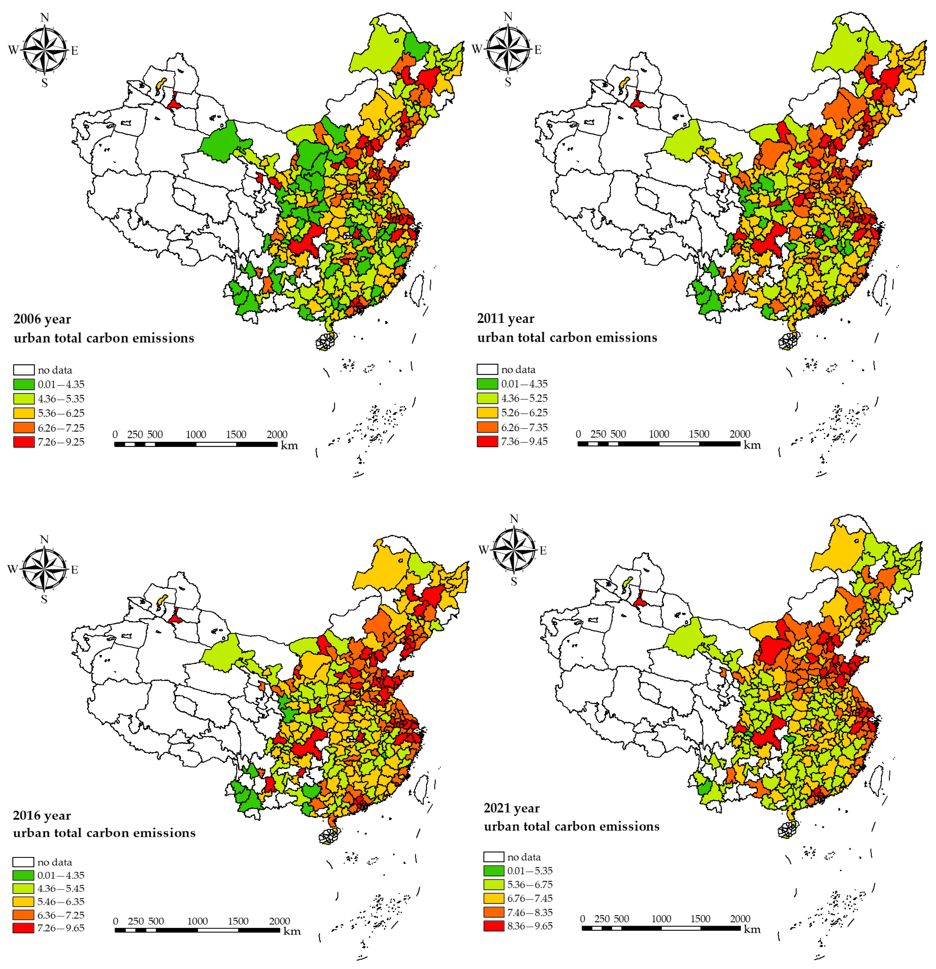
Equation (10) defines CE as the aggregate carbon emissions for a city, where C_g, C_h, C_e, and C_p correspond to emissions derived from four energy sources: natural gas (g), heating (h), electricity consumption (e), and liquefied petroleum gas (p), respectively. E_g, E_h, E_e, and E_p denote the consumption for these four energy sources during 2006–2021, respectively. κ, χ, φ, and ν are carbon conversion coefficients for natural gas, raw coal, electricity, and liquefied petroleum gas, respectively. In line with IPCC recommendations, the emission coefficients are 1.9003 kgCO₂/kg for raw coal, 3.1013 kgCO₂/m³ for liquefied petroleum gas, and 2.1622 kgCO₂/m³ for natural gas. Carbon emissions stemming from electricity consumption are difficult to assess, particularly after 2011, when China segmented its power grid into six areas: eastern, northern, central, southern (Hainan was merged into the southern grid), northeastern, and northwestern. Therefore, we evaluated the carbon emissions generated by electricity use in each region based on the historical CO₂ emission baseline in China. Chinese urban carbon emissions in 282 cities during 2006–2021 are illustrated in Figure 2.

4.2.2. Core Explanatory Variable: Energy Saving and Emission Reduction (ESER) City Pilot

Relying on the official pilot city list issued by China’s Ministry of Finance in conjunction with the National Development and Reform Commission, this study constructs a policy treatment variable. Specifically, more precisely, when a city becomes a demonstration city in year t, its value is given a value of 1 for year t and subsequent years; otherwise, it is assigned 0. We remove Haidong from the sample to maintain statistical uniformity, as it upgraded from district- to prefecture-level city status in 2013. Ultimately, the dataset comprises 282 prefecture-level cities, including 29 pilot cities.

4.2.3. Control Variables

To mitigate coefficient bias and endogeneity arising from omitted variables, this study incorporates urban control variables into the DID model during regression construction, including economic openness level (Openn), industrialization level (Indust), fiscal support (Spend), financial development level (Financ), economic development level (Econo), and population density (Densi). Specifically, the economic openness level (Openn) represents the proportion of total imports and exports relative to GDP. The industrialization level (Indust) is the share of the value added by the secondary industry to the regional GDP. Fiscal support (Spend) is expressed as the proportion of science and technology spending, as well as education spending, in fiscal expenditure to GDP. The financial development level (Financ) is represented by the ratio of the loan balance of financial institutions to GDP for each city. The urban economic development level (Econo) refers to the per capita regional gross domestic product in each city. Population density (Densi) denotes permanent resident density in the administrative region of each city.

4.3. Data Sources and Description

It is well acknowledged that the availability and validity of data are basic premises for conducting empirical research. Accordingly, we carefully matched the ESER pilot city list with corresponding city-level data to construct a novel panel dataset spanning 2006–2021. After excluding cities with substantial missing data, the final sample consists of 282 prefecture-level cities across 30 provincial-level administrative regions in China. The primary data sources include the China Statistical Yearbook, the EPS database, and the China Urban Statistical Yearbook. To estimate urban carbon emissions, additional data were collected from the China Urban–Rural Construction Statistical Yearbook and the China Energy Statistical Yearbook. For the missing values in certain years, linear interpolation and ARIMA prediction techniques were applied to fill them in. Furthermore, to mitigate heteroskedasticity, continuous variables were winsorized at the 1% quantile through a Winsor 2 truncation approach. Moreover, all absolute variables have been logarithmized, yielding 4512 observations, as indicated in

Table 1. Descriptive statistics.

Variable	Definition	The Whole Sample				Pilot Cities		Non-Pilot Cities
		SD	Mean	Obs	VIF	SD	Mean	SD	Mean
CE	Urban carbon emissions	1.186	6.251	4512	—	1.204	7.077	1.147	6.156
Fiscal_did	ESER pilot city policy	0.236	0.059	4512	1.07	0.495	0.573	0	0
Densi	Population density	0.923	5.737	4512	1.14	0.725	5.932	0.941	5.715
Indust	Industrialization level	0.077	0.381	4512	1.57	0.078	0.374	0.077	0.382
Spend	Fiscal support	0.017	0.036	4512	1.58	0.012	0.032	0.017	0.036
Financ	Financial development	0.250	0.631	4512	1.69	0.312	0.735	0.239	0.619
Econo	Economic development	0.718	10.490	4512	1.75	0.658	10.757	0.718	10.460
Openn	Economic openness level	0.276	0.192	4512	1.11	0.336	0.262	0.267	0.184

. In addition, the VIF values of all variables are less than 10, confirming that multicollinearity is not a concern in our models.

5. Empirical Results and Analysis

5.1. Baseline Regression Analysis

Urban carbon emissions are designated as dependent variables in this analysis, with ESER identified as the primary independent variable.

Table 2. Baseline panel regression estimates for ESER’s impact on CE and PCE.

Variable	CE							PCE
	(1)	(2)	(3)	(4)	(5)	(6)	(7)	(8)
Fiscal_did	−0.283 ***	−0.225 ***	−0.226 ***	−0.233 ***	−0.234 ***	−0.232 ***	−0.233 ***	−0.125 ***
	(−7.54)	(−6.22)	(−6.25)	(−6.43)	(−6.46)	(−6.39)	(−6.41)	(−6.03)
Econo		0.643 ***	0.677 ***	0.673 ***	0.662 ***	0.677 ***	0.676 ***	0.075 ***
		(18.91)	(17.11)	(17.01)	(15.97)	(15.82)	(15.82)	(3.09)
Indust			−0.332 *	−0.366 *	−0.382 *	−0.367 *	−0.343 *	−0.290 **
			(−1.67)	(−1.84)	(−1.91)	(−1.83)	(−1.71)	(−2.53)
Densi				0.335 ***	0.334 ***	0.329 ***	0.303 ***	−0.151 **
				(3.00)	(2.99)	(2.94)	(2.67)	(−2.33)
Financ					−0.058	−0.066	−0.063	−0.122 ***
					(−0.89)	(−1.00)	(−0.96)	(−3.25)
Spend						1.375	1.557	−0.473
						(1.41)	(1.58)	(−0.84)
Openn							−0.057	−0.002
							(−1.28)	(−0.07)
_Cons	6.268 ***	−0.481	−0.708 *	−2.577 ***	−2.412 ***	−2.589 ***	−2.444 ***	1.335 ***
	(1037.82)	(−1.35)	(−1.85)	(−3.53)	(−3.20)	(−3.39)	(−3.16)	(3.03)
ID Fixed	Yes	Yes	Yes	Yes	Yes	Yes	Yes	Yes
Time Fixed	Yes	Yes	Yes	Yes	Yes	Yes	Yes	Yes
R2	0.899	0.907	0.907	0.907	0.907	0.907	0.907	0.912
F statistic	56.84	209.6	140.7	108.0	86.53	72.46	62.35	11.16
Obs	4512	4512	4512	4512	4512	4512	4512	4512

Note: t-statistics in parentheses. Asterisks denote statistical significance: *** p < 0.01, ** p < 0.05, * p < 0.1.

reports the detailed empirical outcomes for Model (9).

As is well known, the regression outcome of Fiscal_did is −0.283 without adding any control variables, passing the 1% significance test in Column (1). From Columns (2) to (7), control variables such as fiscal support (Spend), financial development (Financ), and economic development (Econo) are gradually introduced, and the results for ESER (Fiscal_did) remain significant at the 1% level. Fiscal_did for CE is −0.233, as reported in Column (7), which indicates that when Fiscal_did increases by one standard deviation, carbon emissions (CE) decrease by about 0.046 (= 0.233 × 0.236/1.186) standard deviations. A reasonable explanation is that ESER reduces energy consumption through fiscal subsidies and tax incentives, namely, encouraging enterprises to apply energy-conserving technologies, thereby curtailing carbon emissions. Overall, establishing ESER pilot zones contributes to lowering urban carbon emissions, consistent with Xu et al. [44]. Furthermore, when per capita carbon emissions (PCE) are selected as an explained variable in Model (9), as exhibited in Column 8, Fiscal_did for PCE is significant at −0.125, thereby validating Hypothesis 1 (H1).

5.2. Robustness Analysis

5.2.1. Parallel Trend Testing

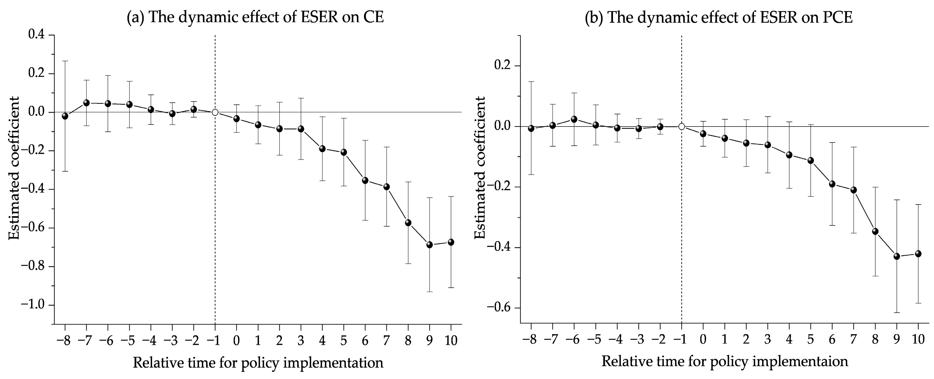
To examine whether pilot and non-pilot cities exhibited comparable CE patterns before ESER’s introduction, we conducted parallel trend tests on CE and PCE, as illustrated in Figure 3.

Figure 3 illustrates the parallel trend tests comparing carbon emissions trends between treatment and control groups. We set the first period before ESER pilot zones’ establishment as a baseline, detecting that neither CE nor PCE values displayed statistical significance before the policy took effect, which verifies the validity of the parallel trend hypothesis. Moreover, Figure 3 further reveals ESER’s dynamic effects following implementation. Specifically, after the establishment of ESER pilot zones, CE began to be significantly negatively affected in the fourth year, while PCE began to indicate negative effects in the sixth period. The sustained reduction in urban carbon emissions observed in pilot zones confirms ESER’s effective role in lowering carbon emissions.

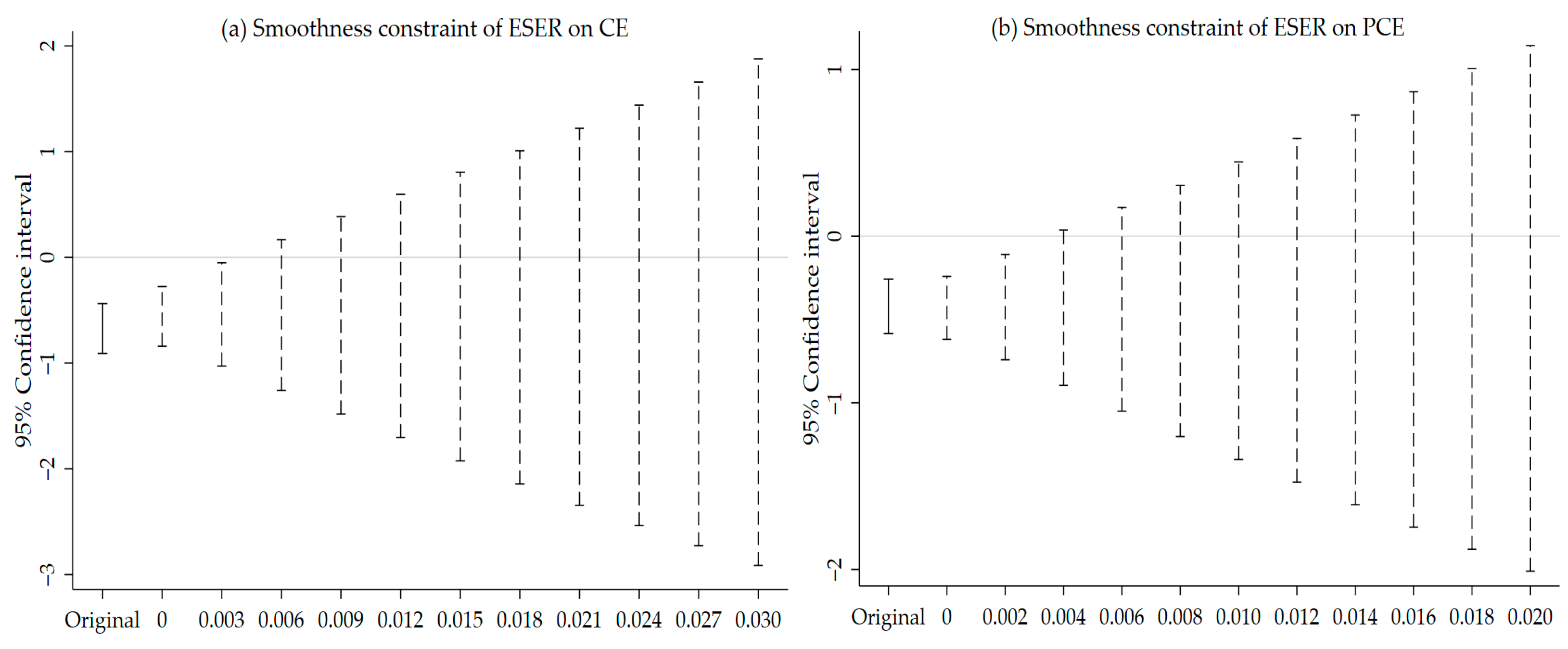
Furthermore, to assess how slight deviations from the parallel trends assumption impact our estimation results, we conducted a sensitivity analysis following Biasi and Sarsons [45]. The findings are presented in Figure 4, where smooth constraint conditions of ESER for CE and PCE are shown in Figure 4a and Figure 4b, respectively. These outcomes indicate that, even allowing for a certain degree of deviation from parallel trends, ESER still has a significant effect.

5.2.2. Placebo Testing

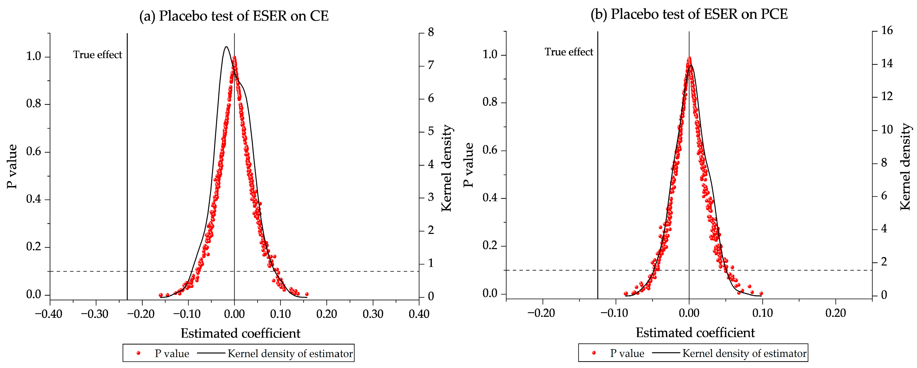
To rule out false policy effects driven by random factors and to be more precise, we followed the approach of Beck et al. [46] and implemented a placebo test, with the results presented in Figure 5.

Secondly, to alleviate estimation bias originating from random factors in this model, we further validated its effectiveness using placebo testing. To be specific, we randomly select 29 cities as a pseudo-treated group, with the remaining cities forming a pseudo-control group. We generated Fiscal_did, a pseudo policy dummy, through repeatedly sampling 500 times. Figure 5 depicts how these estimated coefficients, along with p-values for pseudo Fiscal_did for CE and PCE, are mainly concentrated near zero and are much larger than the benchmark regression findings. In other words, their kernel density distribution aligns well with a normal distribution. Furthermore, most p-values exceed 0.1, suggesting no significance at the 10% threshold, which supports the idea that reductions in urban carbon emissions are largely attributable to ESER’s program rather than other random factors.

5.2.3. Policy Uniqueness Test

Since some policies were launched during the study period that may have cross-effects with ESER, we conducted a policy uniqueness test to improve the credibility of causal inference and eliminate interference from other policies.

In detail, four additional policies were incorporated for CE and PCE during 2006–2021: the new energy demonstration city policy (Energy_did) performed in 2014 to promote renewable energy adoption, the pilot zones policy for green finance reform and innovation (Green_did) established in 2017 to incentivize sustainable investments, the low-carbon city pilot policy (Low_did) initiated in 2010 to test integrated emission reduction strategies, and the environmental protection tax policy (Tax_did) implemented in 2018 to internalize pollution costs. To isolate the causal effect of ESER from potential contamination by concurrent policies, we augmented Model (9) with four time-varying policy controls.

Table 3. Uniqueness test results for CE and PCE.

Variable	CE					PCE
	(1)	(2)	(3)	(4)	(5)	(6)
Fiscal_did	−0.239 ***	−0.230 ***	−0.222 ***	−0.227 ***	−0.218 ***	−0.120 ***
	(−3.13)	(−3.02)	(−2.89)	(−2.89)	(−2.87)	(−5.82)
Energy_did	−0.137 **				−0.136 **	−0.040 ***
	(−2.18)				(−2.25)	(−2.61)
Green_did		−0.334 ***			−0.374 ***	−0.089 **
		(−2.78)			(−3.64)	(−2.27)
Low_did			−0.073		−0.082 *	−0.017
			(−1.62)		(−1.88)	(−1.34)
Tax_did				−0.155 **	−0.168 **	−0.094 ***
				(−2.23)	(−2.42)	(−6.43)
_Cons	−2.662	−2.643	−2.525	−3.307 *	−3.906 **	0.680
	(−1.49)	(−1.43)	(−1.37)	(−1.75)	(−2.09)	(1.52)
Control	Yes	Yes	Yes	Yes	Yes	Yes
ID Fixed	Yes	Yes	Yes	Yes	Yes	Yes
Time Fixed	Yes	Yes	Yes	Yes	Yes	Yes
R2	0.907	0.907	0.907	0.908	0.909	0.913
F statistic	11.55	10.89	10.93	11.18	10.05	12.00
Obs	4512	4512	4512	4512	4512	4512

Note: t-statistics in parentheses. Asterisks denote statistical significance: *** p < 0.01, ** p < 0.05, * p < 0.1.

presents the ESER estimates after isolating other contemporaneous interventions, addressing potential policy interference. Notably, in Column (1), the Energy_did for carbon emission is controlled, and the sustained negative significance of Fiscal_did reinforces the reliability of our primary findings. Column (2) evaluates ESER’s performance while controlling Green_did. Notably, the coefficient is −0.230 and significant, demonstrating that ESER maintains carbon emission reduction even after neutralizing the potential influence of these interventions. Column (3) assesses the ESER effect under Low_did. The analysis indicates that ESER’s ability to mitigate carbon emissions remains robust after isolating the policy’s effects. Column (4) examines ESER in the context of Tax_did. Strikingly, ESER continues to exhibit a statistically significant negative effect on CE. All four aforementioned policies are included in Column (5), further validating the stability of baseline regression findings. Finally, Column (6) shifts the focus to Fiscal_did for PCE. The findings reaffirm that the ESER scheme exerts a substantial negative impact on PCE, corroborating ESER’s overall effectiveness.

5.2.4. Other Robustness Tests

In addition, to strengthen our findings’ reliability and to address potential concerns related to data selection, model specification, and outcome interpretation, we adopt six complementary approaches to validate the robustness of how ESER impacts CE in the benchmark regression. These methods, along with their outcomes, are noted in

Table 4. Robustness test results for ESER of CE.

Variable	Exclude Expectation	CE_GDP	PSM-DID	Adjust Interval	Adjust Sample	Lagged Control	IV_Air Estimation	IV_River Estimation
	(1)	(2)	(3)	(4)	(5)	(6)	(7)	(8)
Fiscal_did	−0.216 ***	−0.113 ***	−0.196 **	−0.191 ***	−0.210 **	−0.231 ***	−0.228 ***	−0.311 ***
	(−3.38)	(−2.90)	(−2.52)	(−2.89)	(−2.00)	(−3.05)	(−2.90)	(−4.29)
Fiscal_did_f1	−0.017
	(−0.85)
Fiscal_did_f2	−0.002
	(−0.04)
_Cons	−2.441	1.097 *	−0.168	−0.619	−3.674 *	−2.766	—	—
	(−1.33)	(1.69)	(−0.08)	(−0.32)	(−1.71)	(−1.44)	—	—
Control	Yes	Yes	Yes	Yes	Yes	Yes	Yes	Yes
ID Fixed	Yes	Yes	Yes	Yes	Yes	Yes	Yes	Yes
Time Fixed	Yes	Yes	Yes	Yes	Yes	Yes	Yes	Yes
R2	0.907	0.765	0.891	0.912	0.889	0.905	—	—
CD-Wald-F							1.5 × 106	2.0 × 104
KP-rk-LM							35.161	111.681
F statistic	9.56	5.38	4.34	6.58	11.02	11.70	11.62	13.26
Obs	4512	4512	3184	3384	4032	4230	4512	4512

Note: t-statistics in parentheses. Asterisks denote statistical significance: *** p < 0.01, ** p < 0.05, * p < 0.1.

.

First, given that relevant information about ESER was released ahead of the policy’s official enactment, to diminish the estimation bias caused by this expectation, we embedded the variables of one year before (Fiscal_did_f1) and two years before (Fiscal_did_f2) ESER’s implementation in Equation (9) to respectively re-estimate how ESER impacts carbon reduction effect, as represented in Column (1). Fiscal_did for CE is significant at −0.216, while Fiscal_did_f1 and Fiscal_did_f2 are not statistically significant, indicating that the decline in carbon emissions is primarily from ESER, rather than being driven by market participants’ early expectations of ESER changes, effectively excluding the interference of expectation effects on the estimation results.

Second, we substituted our primary carbon emission measure with carbon intensity, consistent with an indicator used by Xu and Liu [41], defined as CO₂ emissions per unit of GDP. Column (2) presents the results using this variable, revealing a statistically significant negative ESER coefficient of −0.113, confirming that our core findings are not sensitive to the measurement of the dependent variable.

Third, we adopted the PSM-DID strategy to construct matched samples between treatment and control groups, thereby reducing potential bias arising from heterogeneity, as noted in Column (3). Specifically, a logit model incorporating a set of control variables was employed to estimate each city’s propensity score. Treated cities were matched to untreated counterparts with the nearest propensity scores, facilitating comparability in covariate characteristics. To enhance the estimation reliability, observations that could not be matched to either the treated group or the untreated group were further eliminated. With a coefficient of −0.196 for CE, ESER is consistent with our baseline results in both sign and direction.

Fourth, given policy diffusion lags and contemporaneous shocks, the sample period was truncated to exclude both the policy initiation phase and extreme events. As evidenced in Column (4), ESER’s estimated value is −0.191 in 2008–2019, confirming our results are not driven by endpoint anomalies or adoption lags.

Fifth, to assess whether our results are driven by privileged administrative cities possessing distinct advantages in economic influence and technological effect, we performed a sub-sample analysis excluding municipalities, which included Beijing, Tianjin, Shanghai, and Chongqing, as well as 26 provincial capitals. As shown in Column (5), this ESER outcome remains at −0.210, demonstrating robust policy effects beyond administrative centers.

Sixth, we dealt with potential simultaneity bias by lagging all control variables by one temporal period. This specification, displayed in Column (6), yields an ESER coefficient of −0.231, proving that the outcomes are not driven by reverse causality and the policy effect persists meaningfully.

Seventh, an instrumental variable (IV_air) approach was applied to handle endogeneity concerns, adopting the air circulation value following Xu and Liu [41]. As evidenced in Column (7), Fiscal_did for CE is significant at −0.228. There are two main reasons. First, the air circulation value reflects the strength of airflow in a region, which is typically determined by factors such as wind speed, topography, and atmospheric pressure. In cities with lower air circulation coefficients, pollutants such as CO₂ and PM₂.₅ are prone to accumulate and linger, resulting in higher concentrations. These cities are more likely to be included in the ESER pilot cities. More importantly, the air circulation value is a climate-related variable that is not subject to manipulation by local governments, and it does not directly or indirectly, through other channels, affect the effectiveness of ESER implementation.

Finally, considering political–economic factors, development priorities, and environmental governance capabilities that may simultaneously influence the selection of ESER policies and air quality management, we introduced an interaction term between the logarithm of municipal river length and the logarithm of national power generation capacity from 2005 to 2020 as a panel data instrumental variable (IV_river). This selection of this variable was based on two considerations. First, river density is highly correlated with urban water area, and cities with larger water areas tend to receive more stringent government oversight, increasing their likelihood of being selected as ESER pilot cities. This satisfies the relevance condition for this instrument. Second, as a geographical endowment variable, river distribution is determined at the natural level and does not directly impact carbon emissions through other economic channels, thus fulfilling the exogeneity principle. As shown in Column (8), Fiscal_did for CE displays a significant −0.311 coefficient, further demonstrating the robustness of ESER’s carbon reduction effects.

5.2.5. Bacon Decomposition

When utilizing a two-way fixed effect approach to evaluate how ESER influences carbon emissions, if there is treatment time heterogeneity, it may lead to biased estimates. To identify where potential bias may arise, as well as assess how much each sub-estimation contributes, we referred to Goodman–Bacon [47] and decomposed the estimation results of ESER for carbon emission derived from Model (9), as summarized in

Table 5. Bacon decomposition results.

Testing Type	Estimator	Weight
Timing_groups	0.1055	0.0163
Never_v_timing	−0.2901	0.9686
Within	3.0967	0.0151

. The overall TWFE estimate can be decomposed into several two-group comparisons, which fall into three categories. These include comparisons where groups treated earlier serve as controls for groups treated later, those where later-treated groups act as controls for earlier-treated groups, and contrasts between untreated and treated groups. Among them, the first type of situation leads to estimation bias. The decomposition outcome of the estimations, including the first and second categories, is 0.1055, but the weight is 0.0163, indicating that it has a small impact on the overall estimation. The third category of estimation is −0.2901, and its weight is 0.9686, which has the greatest influence on the overall results. Therefore, to the best of our knowledge, this benchmark regression outcome is credible.

5.3. Heterogeneity Tests

China’s geographical diversity and uneven resource distribution have sparked substantial differences across regions in resource endowments, development paths, and innovation capabilities, resulting in significant disparities in carbon emission levels and structures. Therefore, it is vital to delve into whether there are differentiated influence effects of ESER in various cities from multiple dimensions to identify the boundary conditions and applicable scope of ESER. In particular, the heterogeneity tests are from four aspects comprising economy attributes, population attributes, innovation attributes, and industrial attributes. The regression outcomes are stated in

Table 6. Heterogeneity test results for ESER of CE.

Variable	Economy Attribute		Population Attribute		Innovation Attribute		Industrial Attribute
	Eco	Others_Eco	Lar	Others_Lar	Innov	Others_Inn	Non-Old	Old_Ind
	(1)	(2)	(3)	(4)	(5)	(6)	(7)	(8)
Fiscal_did	−0.160 **	−0.232	−0.169 **	−0.227	−0.168 **	−0.151	−0.296 ***	0.032
	(−2.33)	(−1.08)	(−2.18)	(−1.48)	(−2.37)	(−1.13)	(−3.29)	(0.28)
_Cons	3.636 *	−8.329 ***	2.044	−9.594 ***	7.493 ***	−8.668 ***	1.853	−3.690 *
	(1.67)	(−3.26)	(0.86)	(−4.18)	(3.81)	(−4.11)	(0.79)	(−1.67)
Control	Yes	Yes	Yes	Yes	Yes	Yes	Yes	Yes
ID Fixed	Yes	Yes	Yes	Yes	Yes	Yes	Yes	Yes
Time Fixed	Yes	Yes	Yes	Yes	Yes	Yes	Yes	Yes
R2	0.900	0.867	0.939	0.852	0.931	0.862	0.921	0.883
F statistic	2.63	13.47	4.60	13.32	3.85	13.41	9.87	18.50
Obs	2256	2256	2208	2304	1200	3312	2992	1520

Note: Cities are classified as follows: (1) “Eco” and “Others_Eco” are divided by median per capita GDP in 2006, with “Eco” denoting cities above this median. (2) “Lar” and “Others_Lar” are classified based on whether a city’s municipal district population exceeded one million in 2014, in line with the State Council’s official policy document. (3) “Innov” and “Others_Inn” follow the official list of national innovative cities issued by the Ministry of Science and Technology. (4) “Old_Ind” and “Non-Old” are defined according to the State Council’s designation of old industrial base cities. t-statistics in parentheses. Asterisks denote statistical significance: *** p < 0.01, ** p < 0.05, * p < 0.1.

, spanning Columns (1) to (8). Moreover, the specific classification criteria are shown in footnotes.

For economic development, when grouped by the median per capita GDP in 2006, our full sample forms two distinct categories: 141 economically more developed cities (Eco) and 141 economically less developed cities (Others_Eco), with the corresponding results displayed in Columns (1)–(2). To the best of our knowledge, the estimated outcome of Fiscal_did for CE is significant at −0.160 for cities located in Eco, while the findings of ESER implementation for CE are negligible for cities in Others_Eco. To be specific, the possible reasons are that cities in more economically developed regions have a high proportion of tertiary industries, and the industrial structure is dominated by high-tech industries and low-energy-consuming services. Moreover, ESER enables Eco, which has a higher proportion of clean energy in its energy consumption, to enhance carbon reduction efforts by refining its energy structures.

Secondly, how demographic characteristics impact technological advancement and energy consumption patterns may lead to significant inter-city disparities in carbon emissions. Referring to Xu et al. [48], we stratified the dataset into two subgroups using a 2014 municipal district population threshold of one million. This classification identified 138 large cities (Lar) as well as 144 other cities (Others_Lar). Contrasted with small and medium cities in Column (4), Column (3) demonstrates that ESER can reduce carbon mitigation in Lar. To the best of our knowledge, the reason is that high population density promotes efficient patterns of resource utilization and energy consumption, forming scale economies. Frequent population mobility and labor optimization brought by a larger population size improve industrial structure upgrading. Meanwhile, higher environmental awareness boosts the popularization of low-carbon behavior. These factors enable big cities to respond to and implement ESER policies more effectively, thus significantly reducing carbon emissions.

Thirdly, guided by the Chinese government’s official list, we classified 75 cities as national innovative cities (Innov) along with 207 as non-national innovative cities (Others_Inn), as reported in Columns (5)–(6). The estimated outcome of Fiscal_did for CE is −0.168 and reaches statistical significance, as displayed in Column (5). That is to say, ESER effectively curbs carbon emissions in Innov. In contrast, the policy impact is statistically insignificant in non-national innovative cities. A plausible explanation is that national innovative cities (Innov) generally possess stronger capabilities in technological R&D and converting innovation achievements into practical applications compared with non-national innovative cities (Others_Inn), reducing environmental protection costs.

Fourthly, for industrial development, we bifurcated the sample into two distinct categories: 95 old industrial base cities (Old_Ind) and 187 non-old industrial base cities (Non-Old), with the corresponding results displayed in Columns (7)–(8). The estimated value of Fiscal_did for CE in non-old industrial base areas is significant at −0.296, indicating a substantial inhibitory effect of ESER in these cities, while no such effect is observed in old industrial base zones. One possible explanation is that, compared with Non-Old, Old_Ind have higher green transformation costs stemming from their historical reliance on heavy industry as well as outdated energy structures, which could limit ESER policies’ effectiveness.

5.4. Transmission Mechanism Analysis

What is the transmission pathway for ESER reducing CE? To clarify the logical chain, we focus on the mechanism test covering energy consumption, green innovation, and industrial upgrading illustrated in Columns (1) to (8) in

Table 7. Mechanism test results for ESER of CE.

Variable	Energy Consumption			Industrial Upgrading			Green Innovation
	Energy	Energy	CE	Ind_up	Ind_up	CE	Patent	Patent	CE
	(1)	(2)	(3)	(4)	(5)	(6)	(7)	(8)	(9)
Fiscal_did	−0.061 ***	−0.029 **		0.102 ***	0.064 ***		0.084 ***	0.059 ***
	(−4.85)	(−2.44)		(7.59)	(6.23)		(10.10)	(7.82)
Fiscal_did_high			−0.195 ***			−0.217 ***			−0.375 ***
			(−3.17)			(−5.22)			(−8.81)
Fiscal_did_low			0.238 *			−0.009			0.420 ***
			(1.95)			(−0.11)			(2.94)
_Cons	1.324 ***	0.677 ***	−2.417 ***	0.734 ***	−0.719 ***	−2.568 ***	0.101 ***	−0.817 ***	−2.567 ***
	(658.52)	(2.69)	(−3.22)	(339.52)	(−3.29)	(−3.43)	(75.88)	(−5.12)	(−3.45)
Control	No	Yes	Yes	No	Yes	Yes	No	Yes	Yes
ID Fixed	Yes	Yes	Yes	Yes	Yes	Yes	Yes	Yes	Yes
Time Fixed	Yes	Yes	Yes	Yes	Yes	Yes	Yes	Yes	Yes
Wald statistic			10.03			4.84			28.49
			[0.0015]			[0.0279]			[0.0000]
R2	0.938	0.945	0.660	0.886	0.935	0.661	0.731	0.783	0.666
F statistic	23.56	85.42	393.8	57.66	464.80	395.6	101.9	163.0	403.7
Obs	4512	4512	4512	4512	4512	4512	4512	4512	4512

Note: t-statistics in parentheses. Asterisks denote statistical significance: *** p < 0.01, ** p < 0.05, * p < 0.1.

. Specifically, we regressed Fiscal_did on each of the three mechanism variables, both with and without the control variables, to evaluate the robustness of these mechanisms. Furthermore, grounded in the 75% and 25% of each mechanism quantile, the full sample was split into a high group (Fiscal_did_high) and a low group (Fiscal_did_low). Concretely, urban energy consumption (Energy) was proxied by per capita energy use to measure energy intensity at the city level. This energy consumption was estimated by extrapolating from the established linear relationship between nighttime light intensity and provincial energy consumption. Additionally, industrial upgrading (Ind_up) was determined by the value-added ratio of the tertiary to secondary sectors, illustrating the structural shift toward a more service-oriented economy. Green innovation capacity (Patent) was gauged using the number of urban green invention patent applications per 10,000 people, which reflects the innovation intensity in sustainable technologies.

First, we see that this ESER scheme’s estimated value in Column (1) is significant at −0.061, which demonstrates that ESER effectively reduces energy consumption across various cities. After adding the control variables, the outcome of Fiscal_did is significant at −0.029, as reported in Column (2). As outlined in Column (3), the value of Fiscal_did_high is evidently −0.195. In contrast, the outcome for Fiscal_did_low is 0.238 and statistically insignificant. Given that the Wald test rejects the null hypothesis, the grouping is plausible for statistical significance, further bolstering Hypothesis 2 (H2).

Second, to assess whether Ind_up helps reduce CE, we refer to the estimates in Columns (4)–(6). The estimated values of 0.102 and 0.064 in Columns (4)–(5), respectively, reflect that ESER has fostered favorable conditions for industrial upgrading by accelerating industrial transformation, concurring with the outcome of Zhou and Lin [26]. By the same token, Fiscal_did_high for CE is notably −0.217 in Column (6), underscoring its positive role in reinforcing carbon mitigation through urban industrial restructuring, and thereby validating Hypothesis 3 (H3).

Third, as is well known, the ESER scheme’s estimated values are significant at 0.084 and 0.059, as in Columns (7)–(8), respectively, which demonstrates that ESER effectively stimulates green innovation activities in cities, endorsing Hypothesis 4 (H4) as well as aligning with Sun and Feng [9]. Namely, as stated in Column (9), the outcome of Fiscal_did_high is notably −0.375, while the value for Fiscal_did_low of CE is 0.420 and statistically insignificant, suggesting that the high Fiscal_did group achieves greater emission reduction effects than the low group.

6. Spatial Spillover Effects Analysis

6.1. Spatial Autocorrelation Test

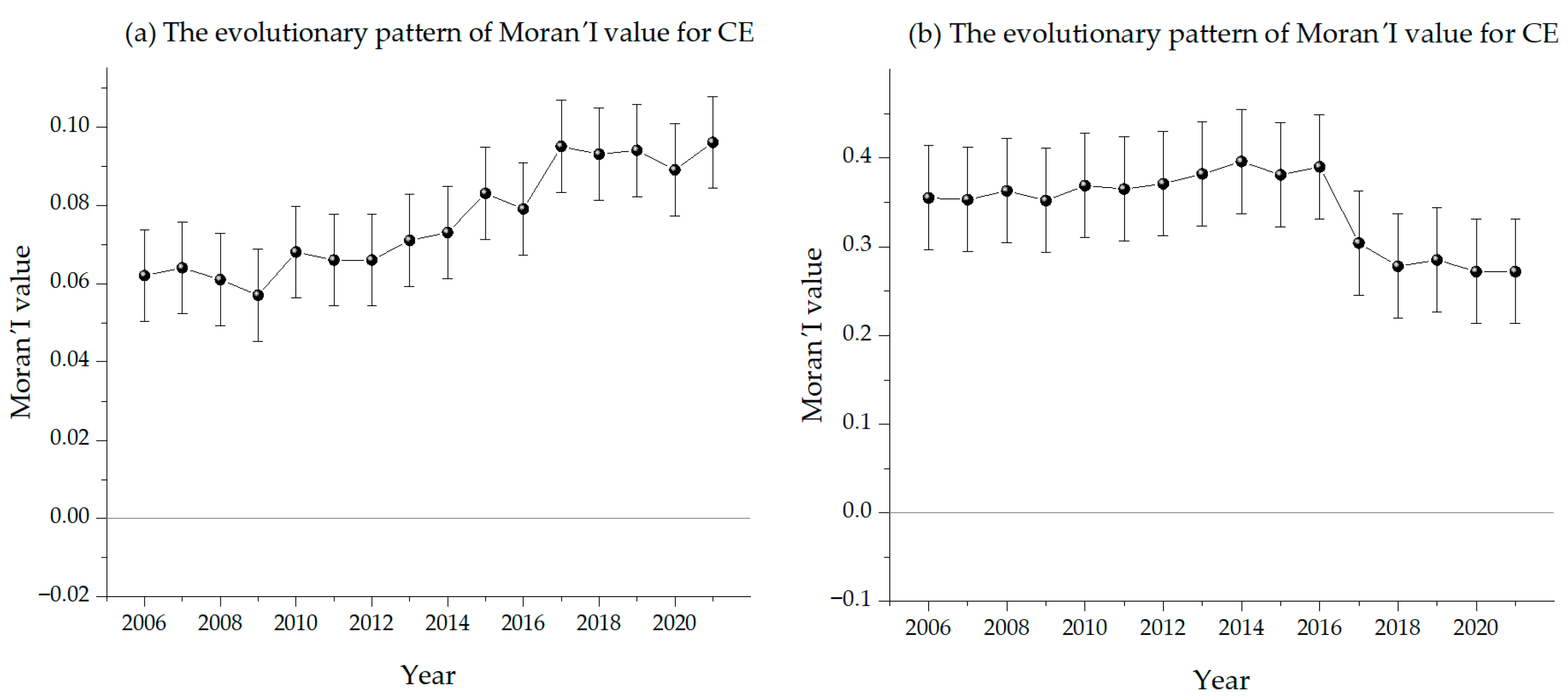
Given interactions in regional economic activities, a carbon emission increase in one area could elevate emission levels in neighboring regions, manifesting a pronounced spatial distribution pattern. That is to say, if one area increases its carbon emissions due to regional economic activities, it can also raise emissions in nearby areas, showing a clear pattern of how emissions are spread out. To probe this spatial correlation across cities, following Baysoy and Altug [49], a geographic weight matrix was constructed based on both longitude and latitude in 282 cities, and Moran’s I index was applied to execute global spatial autocorrelation (depicted in Figure 6a). For this geographic spatial weight matrix, we adopted an inverse distance method based on the longitude and latitude coordinates of the city. To be more specific, this spatial weight w_ij is defined as the reciprocal of the spherical distance d_ij between cities i and j, calculated by 1/d_ij, where d_ij is determined by the latitude and longitude of two centroids. Furthermore, to compare spatial autocorrelation patterns across matrices, an economic weight matrix was adopted (depicted in Figure 6b). Referring to Lin et al. [50], we constructed an economic spatial weight matrix based on 2006–2021 per capita GDP data for 282 cities. More precisely, we computed the absolute GDP differences between two cities, taking the inverse of these values to form the initial weight matrix (setting weights to zero where the difference is zero), and applied row standardization to obtain the final normalized economic weight matrix.

In general, Moran’s I indices remain consistently greater than zero during 2006–2021 and reach significance with a 95% confidence interval, as indicated by Figure 6, revealing that this is spatial clustering rather than randomly distributed, confirming that using a spatial econometric model is suitable for subsequent analyses. These spatial autocorrelation findings for CE indicate that carbon emissions across different regions often exhibit certain similarities. That is to say, we should consider their spatial spillover effects. It is worth noting that there is a smaller standard deviation from the means for Figure 6b compared to Figure 6a. A possible reason is that cities with similar economic characteristics often share strong similarities in terms of industrial development, thereby exhibiting more homogeneous carbon emission behaviors over time. In contrast, geographically proximate cities may differ significantly in economic development level, industrial structure, and other aspects, leading to greater fluctuations in the spatial clustering of their carbon emission patterns.

6.2. Spatial Panel Regression Findings

To further investigate the spatial dynamics of ESER’s impact, a two-way fixed effects spatial autoregressive (SAR) model was employed to analyze how ESER impacts carbon emissions.

As shown in

Table 8. Spatial panel regression for ESER of CE.

Variable	Geometric Matrix_CE				Economic Matrix_CE
	(1)	(2)	(3)	(4)	(5)	(6)	(7)	(8)
	Main_Geo	Direct_Geo	Indirect_Geo	Total_Geo	Main_Eco	Direct_Eco	Indirect_Eco	Total_Eco
Fiscal_did	−0.240 ***	−0.239 ***	−0.284 ***	−0.524 ***	−0.230 ***	−0.230 ***	−0.068 ***	−0.298 ***
	(−6.88)	(−6.66)	(−2.91)	(−4.41)	(−6.64)	(−6.43)	(−4.77)	(−6.27)
Econo	0.622 ***	0.623 ***	0.736 ***	1.359 ***	0.612 ***	0.615 ***	0.180 ***	0.795 ***
	(14.88)	(15.49)	(3.35)	(6.05)	(14.75)	(15.35)	(7.06)	(14.94)
Indust	−0.225	−0.205	−0.237	−0.441	−0.306	−0.287	−0.084	−0.371
	(−1.16)	(−1.09)	(−1.00)	(−1.06)	(−1.60)	(−1.55)	(−1.50)	(−1.54)
Densi	0.230 **	0.229 **	0.263 **	0.491 **	0.360 ***	0.361 ***	0.106 ***	0.467 ***
	(2.10)	(2.15)	(1.97)	(2.14)	(3.31)	(3.40)	(3.13)	(3.40)
Financ	−0.022	−0.021	−0.025	−0.046	−0.094	−0.094	−0.028	−0.122
	(−0.35)	(−0.33)	(−0.32)	(−0.33)	(−1.50)	(−1.49)	(−1.44)	(−1.48)
Spend	1.562 *	1.626 *	1.948	3.574	0.953	1.017	0.298	1.315
	(1.65)	(1.73)	(1.44)	(1.61)	(1.01)	(1.08)	(1.06)	(1.08)
Openn	−0.077 *	−0.078 *	−0.092	−0.170 *	−0.075 *	−0.077 *	−0.022 *	−0.099 *
	(−1.77)	(−1.74)	(−1.48)	(−1.65)	(−1.76)	(−1.72)	(−1.66)	(−1.72)
ρ	0.534 ***				0.233 ***
	(7.11)				(8.71)
R2	0.445				0.528
Log-Lik	−1639.108				−1622.968
Obs	4512	4512	4512	4512	4512	4512	4512	4512

Note: z-values in parentheses. Asterisk means significance: *** p < 0.01, ** p < 0.05, * p < 0.1.

, Columns (1) and (5) indicate that the spatial estimated outcomes of Fiscal_did on CE are notably −0.240 (Main_Geo) and −0.230 (Main_Eco) across different matrices, which demonstrates that this negative outcome of ESER for CE is evidently robust. Furthermore, Columns (2) to (4) decompose the spatial effects based on a geometric matrix, where the coefficients for the direct effect (Direct_Geo), indirect effect (Indirect_Geo), and total effect (Total_Geo) of Fiscal_did on CE are −0.239, −0.284, and −0.524. Similarly, Columns (6) to (8) decompose the spatial effects based on an economic matrix, where the coefficients for the direct effect (Direct_Eco), indirect effect (Indirect_Eco), and total effect (Total_Eco) of Fiscal_did on CE are −0.230, −0.068, and −0.298. In other words, these findings not only prove the robustness of previous conclusions but also reveal the transmission mechanism of ESER’s carbon reduction effect on surrounding areas through spatial spillover effects. Therefore, the inter-regional linkage and synergy of carbon reduction policies should not be ignored.

6.3. Decay Boundaries for Spatial Spillover Effects

To further explore the spatial extent of the ESER policy’s spillover effects, we conducted a spatial heterogeneity analysis, with the results presented in Figure 7. A radius of 38 km was selected as the minimum radiation distance to examine the attenuation pattern of spillover effects over varying distances. This setting was based on three main considerations. First, by simplifying cities into circular shapes, Zhoushan has the smallest radius among the sampled cities, approximately 38 km, making it suitable for capturing the most immediate and potentially affected areas. Second, spillover mechanisms typically depend on geographic proximity, and a 38 km radius provides a meaningful benchmark to reflect the initial transmission range of the policy. Third, using 38 km as a baseline allows for the division of multiple distance bands, facilitating a systematic analysis of how spillover effects change with increasing distance. For instance, in the pilot cities, Shenzhen and Dongguan are adjacent cities with a distance falling between 38 and 76 km, demonstrating realistic spatial relationships and supporting the policy relevance of this distance-based analysis.

Figure 7 applies a spline-fitting approach to better capture the overall pattern of spatial spillovers, demonstrating that the effective spillover range of ESER for CE and PCE lies between 38 km and 76 km and reaches significance with a 90% confidence interval. Furthermore, the spatial spillover coefficients fluctuate around zero between 76 km and 342 km, with the amplitude of fluctuation gradually stabilizing, which indicates a distinct attenuation pattern of indirect spillover effects. One possible explanation is that the dissemination of policy information and green technologies usually relies on geographical proximity. As the distance increases, the information diffusion cost and resource-sharing difficulty gradually rise, thereby weakening ESER’s spillover effect. In addition, neighboring cities can more easily generate synergistic effects under ESER incentives.

7. Conclusion and Policy Recommendations

ESER offers valuable insights into balancing economic growth and environmental protection, providing practical experience for other developing countries. Using a multi-period DID model with data from 2006–2021, we conclude that ESER significantly reduces urban carbon emissions, averaging a decrease of approximately 23.3% compared to non-pilot cities. Robustness checks, including dynamic effect analysis and instrumental variable methods, confirm these findings. The policy’s effectiveness varies across cities due to differences in economic level, population size, innovation capacity, and industrial structure. Mechanism tests reveal that ESER promotes carbon reduction through reducing energy consumption, optimizing industrial structure, and fostering green innovation. Moreover, it generates positive spillovers in neighboring regions. Based on these results, we offer the following policy recommendations.

First, strengthening environmental regulatory frameworks to better manage carbon emissions, and optimizing the policy coordination mechanism between central and local governments. A standardized and transparent carbon emission monitoring and evaluation system should be established, focusing on high-emission sectors like power, chemical, and transportation industries. Utilizing cutting-edge technologies, including IoT, blockchain, and big data, can facilitate the development of real-time monitoring and dynamic evaluation systems, significantly enhancing the precision of carbon emission data. However, relying solely on technological empowerment is not enough to form an effective governance synergy. To prevent local authorities from excessively focusing on immediate economic growth at the cost of long-term environmental welfare, environmental performance metrics should be integrated into their evaluation systems. By regularly assessing and providing feedback, intrinsic motivation for governance can be stimulated, thereby achieving a decoupling of economic growth from carbon emissions.

Second, given demonstration cities’ implementation of ESER notably reduced urban carbon emissions, both central and local governments should expedite the expansion of pilot zones for ESER. This expansion should be systematically extended to non-pilot cities that meet the criteria, establishing a green fiscal policy system that covers a broader region. Throughout this process, spatial factors should be systematically considered to harness the positive spillover effects of ESER. Through policy radiation, the green transition of surrounding areas can be stimulated, improving coordinated regional carbon reduction development. In addition, the government should enhance the incentive and constraint functions of green finance, employing diversified fiscal tools to unblock the channels of fund circulation and allocation and reasonably facilitate resource allocation toward sectors aligned with ecological sustainability and carbon neutrality initiatives, effectively curbing high-emission and energy-intensive industrial activities to maximize policy execution and ensure optimal carbon reduction outcomes. Furthermore, beyond the pilot phase, China must build a comprehensive climate governance system. This includes enacting a unified climate law, enhancing inter-ministerial coordination, and aligning local policies with national carbon neutrality targets.

Third, when assessing how ESER impacts carbon emissions, it must be assessed with attention to city-level heterogeneity across dimensions like economic status, population density, innovation capacity, and industrial layout. Tailored policies should be implemented to avoid resource misallocation and inefficiencies in reduction associated with a one-size-fits-all management approach. The above research indicates that ESER is more effective in economically developed cities and large cities. Thus, fostering stronger regional connectivity between less developed cities along with major economic hubs should be encouraged to strengthen this interregional linkage with economically developed cities and big cities. By learning from their successful practices in carbon reduction and utilizing policy radiation, experience replication and dissemination can be achieved. Additionally, accelerating energy infrastructure in smaller and underdeveloped cities is fundamental to bolstering their green transition capabilities. For old industrial base cities, the focus should be on adjusting and optimizing industrial structures through restricting high-emission and resource-demanding sectors, along with enabling decarbonized transformation across legacy industrial domains. To address the issue of non-innovative cities where carbon reduction effects are not prominent, investment in green low-carbon technology research should be increased, actively cultivating and attracting technological talent to break through key core technologies. Furthermore, improving the technology transformation mechanism is vital for expanding the share of high-tech sectors in the overall industrial landscape, facilitating the application of low-carbon technologies in actual production.

Fourth, attention should be paid to the roles of reducing energy consumption and optimizing industrial structure, as well as fostering green innovation, when considering ESER’s influence on carbon emissions. To limit energy consumption, the core focus should be on optimizing energy structure to advance supply-side structural reforms, accelerating efforts to harness renewable sources like wind, solar, biomass, and hydroelectric power, and adding low-carbon energy consumption, thereby contributing to a structural shift in the energy system characterized by greener and lower-carbon operations. However, many enterprises are locked into original technologies, struggling to break free from reliance on high-carbon technologies, which increases the cost and uncertainty of green transformation. Thus, the government should construct an innovation compensation mechanism to provide appropriate economic support to enterprises bearing high substitution costs, reducing transformation pressures. For industrial structure upgrading, the core focus should be on integrating structural sophistication with rationalization, and enhancing the decarbonization trajectory of secondary industries through policy-driven transformation while accelerating the development of low-carbon agriculture and modern services, which builds a diversified and collaborative modern industrial system. In addition, green consumption guidance should be strengthened, stimulating demand for low-carbon products and services from the consumer side, which compels enterprises to develop green industries.

Although this study employs both theoretical and empirical methods to analyze ESER’s impact on carbon emissions, two limitations remain. First, due to data limitations, this study adopts fixed IPCC emission coefficients and uses linear interpolation and ARIMA models to address missing energy data. These methods may overlook regional heterogeneity in coal quality, energy structure, and technology levels, potentially affecting the accuracy of carbon emission estimates. Future research could utilize more granular data and advanced imputation techniques, such as machine learning or sensitivity analysis, to enhance robustness. Second, the spatial analysis relies solely on geographic proximity and does not account for other forms of inter-city linkages like transportation infrastructure or economic ties. Additionally, ESER is treated as a binary variable, ignoring potential variation in policy strength and implementation across cities. Future studies should consider incorporating multi-dimensional spatial connections and continuous measures of policy intensity to better capture heterogeneous effects.

References

1. Sufyanullah, K.; Ahmad, K.A.; Sufyan Ali, M.A. Does emission of carbon dioxide is impacted by urbanization? An empirical study of urbanization, energy consumption, economic growth and carbon emissions—Using ARDL bound testing approach. Energy Policy 2022, 164, 112908. [Google Scholar] [CrossRef]
2. Wang, J.Q.; Tian, J.X.; Kang, Y.X.; Guo, K. Can green finance development abate carbon emissions: Evidence from China. Int. Rev. Econ. Financ. 2023, 88, 73–91. [Google Scholar] [CrossRef]
3. Waldinger, M. The Economic Effects of Long-Term Climate Change: Evidence from the Little Ice Age. J. Polit. Econ. 2022, 130, 2275–2314. [Google Scholar] [CrossRef]
4. Lin, B.Q.; Zhu, J.P. Is the implementation of energy saving and emission reduction policy really effective in Chinese cities? A policy evaluation perspective. J. Clean. Prod. 2019, 220, 1111–1120. [Google Scholar] [CrossRef]
5. Wang, Z.L.; Qiu, S.L. Can “energy saving and emission reduction” demonstration city selection actually contribute to pollution abatement in China? Sustain. Prod. Consump. 2021, 27, 1882–1902. [Google Scholar] [CrossRef]
6. Ma, Q.S.; Zhang, Y.M.; Hu, F.; Zhou, H.Y. Can the energy conservation and emission reduction demonstration city policy enhance urban domestic waste control? Evidence from 283 cities in China. Cities 2024, 154, 105323. [Google Scholar] [CrossRef]
7. Wang, K.K.; Yin, R.; He, Q.; Wang, S.H. Transfer payments and carbon reduction in China: The effect of the national comprehensive demonstration city of energy saving and emission reduction fiscal policy. Energy 2024, 297, 131253. [Google Scholar] [CrossRef]
8. Jin, H.; Yang, J.; Chen, Y.Y. Energy saving and emission reduction fiscal policy and corporate green technology innovation. Front. Psychol. 2022, 13, 1056038. [Google Scholar] [CrossRef]
9. Sun, L.; Feng, N. Research on fiscal policies supporting green and low-carbon transition to promote energy conservation and emission reduction in cities: Empirical evidence from China. J. Clean. Prod. 2023, 430, 139688. [Google Scholar] [CrossRef]
10. Acheampong, A.O. Economic growth, CO2 emissions and energy consumption: What causes what and where? Energy Econ. 2018, 74, 677–692. [Google Scholar] [CrossRef]
11. Mirza, F.M.; Kanwal, A. Energy consumption, carbon emissions and economic growth in Pakistan: Dynamic causality analysis. Renew. Sustain. Energy Rev. 2017, 72, 1233–1240. [Google Scholar] [CrossRef]
12. Boutabba, M.A. The impact of financial development, income, energy and trade on carbon emissions: Evidence from the Indian economy. Econ. Model. 2014, 40, 33–41. [Google Scholar] [CrossRef]
13. Shahbaz, M.; Destek, M.A.; Dong, K.Y.; Jiao, Z.L. Time-varying impact of financial development on carbon emissions in G-7 countries: Evidence from the long history. Technol. Forecast. Soc. Change 2021, 171, 120966. [Google Scholar] [CrossRef]
14. Tan, F.F.; Yang, S.S.; Niu, Z.Y. The impact of urbanization on carbon emissions: Both from heterogeneity and mechanism test. Environ. Dev. Sustain. 2023, 25, 4813–4829. [Google Scholar] [CrossRef]
15. Musah, M.; Kong, Y.S.; Mensah, I.A.; Antwi, S.K.; Donkor, M. The connection between urbanization and carbon emissions: A panel evidence from West Africa. Environ. Dev. Sustain. 2020, 23, 11525–11552. [Google Scholar] [CrossRef]
16. Xu, X.P.; Zhu, Y.Q. Towards Green Development: Identifying the Impact of Population Aging on China’s Carbon Emissions Based on the Provincial Panel Data Analysis. Pol. J. Environ. Stud. 2024, 33, 4861–4877. [Google Scholar] [CrossRef] [PubMed]
17. Dalton, M.; O’Neill, B.; Prskawetz, A.; Jiang, L.W.; Pitkin, J. Population aging and future carbon emissions in the United States. Energy Econ. 2008, 30, 642–675. [Google Scholar] [CrossRef]
18. Wan, G.H.; Wang, C.; Wang, J.X.; Zhang, X. The income inequality-CO2 emissions nexus: Transmission mechanisms. Ecol. Econ. 2022, 195, 107360. [Google Scholar] [CrossRef]
19. Hailemariam, A.; Dzhumashev, R.; Shahbaz, M. Carbon emissions, income inequality and economic development. Empir. Econ. 2019, 59, 1139–1159. [Google Scholar] [CrossRef]
20. Han, D.R.; Bi, C.F.; Wu, H.S.; Hao, P. Energy and environment: How could energy-consuming transition promote the synergy of pollution reduction and carbon emission reduction in China? Urban Clim. 2024, 55, 101931. [Google Scholar] [CrossRef]
21. Hu, H.S.; Dong, W.H.; Zhou, Q. A comparative study on the environmental and economic effects of a resource tax and carbon tax in China: Analysis based on the computable general equilibrium model. Energy Policy 2021, 156, 112460. [Google Scholar] [CrossRef]
22. Al Mamun, M.; Boubaker, S.; Nguyen, D.K. Green finance and decarbonization: Evidence from around the world. Financ. Res. Lett. 2022, 46, 102807. [Google Scholar] [CrossRef]
23. Rasoulinezhad, E.; Taghizadeh-Hesary, F. Role of green finance in improving energy efficiency and renewable energy development. Energy Effic. 2022, 15, 14. [Google Scholar] [CrossRef] [PubMed]
24. Li, Z.; Gao, S.; Song, S.F. Can Green Fiscal Policies Drive the Digital Transformation of Enterprises? J. Knowl. Econ. 2024, 1–36. [Google Scholar] [CrossRef]
25. Lee, C.C.; Wang, E.Z.; Tang, H.M. Green fiscal policy and carbon emission: Enterprises’ level evidence from China. Renew. Sustain. Energy Rev. 2024, 203, 114795. [Google Scholar] [CrossRef]
26. Zhou, Y.C.; Lin, B.Q. The energy-saving effect of green fiscal policy: Empirical evidence from China’s comprehensive demonstration cities of energy conservation and emission reduction fiscal policy. Appl. Energy 2025, 378, 124784. [Google Scholar] [CrossRef]
27. Bujunoori, R.R.; Mannil, N.; Tantri, P. Does labor composition impact the transmission of monetary policy to output? J. Dev. Econ. 2024, 167, 103241. [Google Scholar] [CrossRef]
28. Salinas, P.; Solé-Ollé, A. Partial fiscal decentralization reforms and educational outcomes: A difference-in-differences analysis for Spain. J. Urban Econ. 2018, 107, 31–46. [Google Scholar] [CrossRef]
29. Gomes, P.; Librero-Cano, A. Evaluating three decades of the European Capital of Culture programme: A difference-in-differences approach. J. Cult. Econ. 2016, 42, 57–73. [Google Scholar] [CrossRef]
30. Jiang, L.; Zhang, Z.N.; Zhang, B.; He, S.X. Does “National Civilized City” policy mitigate air pollution in China? A spatial Durbin difference-in-differences analysis. BMC Public Health 2024, 24, 1234. [Google Scholar] [CrossRef]
31. Nenavath, S. Impact of fintech and green finance on environmental quality protection in India: By applying the semi-parametric difference-in-differences (SDID). Renew. Energy 2022, 193, 913–919. [Google Scholar] [CrossRef]
32. Miyawaki, A.; Noguchi, H.; Kobayashi, Y. Impact of medical subsidy disqualification on children’s healthcare utilization: A difference-in-differences analysis from Japan. Soc. Sci. Med. 2017, 191, 89–98. [Google Scholar] [CrossRef] [PubMed]
33. Bielen, S. Prosecutors and crime deterrence: Evidence from a difference-in-differences analysis with staggered treatment. J. Crim. Justice 2024, 90, 102147. [Google Scholar] [CrossRef]
34. McGavock, T. Here waits the bride? The effect of Ethiopia’s child marriage law. J. Dev. Econ. 2021, 149, 102580. [Google Scholar] [CrossRef]
35. Xu, H.Z.; Li, X.Y. Effect mechanism of Chinese-style decentralization on regional carbon emissions and policy improvement: Evidence from China’s 12 urban agglomerations. Environ. Dev. Sustain. 2023, 25, 474–505. [Google Scholar] [CrossRef]
36. Zhao, Y.H.; Zhang, Y.Y.; Wang, S.Y. Can a Policy Mix Achieve a Collaborative Effect? Exploring the Nested Implementation Process of Urban Carbon Emission Reduction Policies. Sustainability 2024, 16, 6529. [Google Scholar] [CrossRef]
37. Antweiler, W.; Copeland, B.R.; Taylor, M.S. Is free trade good for the environment? Am. Econ. Rev. 2001, 91, 877–908. [Google Scholar] [CrossRef]
38. Andersen, D.C. Do credit constraints favor dirty production? Theory and plant-level evidence. J. Environ. Econ. Manag. 2017, 84, 189–208. [Google Scholar] [CrossRef]
39. Xu, X.P.; Song, Y.C. Is there a conflict between automation and environment? Implications of artificial intelligence for carbon emissions in China. Sustainability 2023, 15, 12437. [Google Scholar] [CrossRef]
40. Qi, J.; Tang, X.; Xi, X.C. The size distribution of firms and industrial water pollution: A quantitative analysis of China. Am. Econ. J. Macroecon. 2021, 13, 151–183. [Google Scholar] [CrossRef]
41. Xu, X.P.; Liu, L. Effects of climate policy on urban carbon emissions—New insights from China’s Low-Carbon City Pilot policy. Appl. Ecol. Environ. Res. 2025, 23, 3637–3661. [Google Scholar] [CrossRef]
42. Wang, L.; Zhang, N.Y.; Deng, H.G.; Wang, P.F.; Yang, F.; Qu, J.J.; Zhou, X.X. Monitoring urban carbon emissions from energy consumption over China with DMSP/OLS nighttime light observations. Theor. Appl. Climatol. 2022, 149, 983–992. [Google Scholar] [CrossRef]
43. Liang, X.Y.; Fan, M.; Xiao, Y.T.; Yao, J. Temporal-spatial characteristics of energy-based carbon dioxide emissions and driving factors during 2004–2019, China. Energy 2022, 261, 124965. [Google Scholar] [CrossRef]
44. Xu, T.T.; Kang, C.Y.; Zhang, H. China’s efforts towards carbon neutrality: Does energy-saving and emission-reduction policy mitigate carbon emissions? J. Environ. Manag. 2022, 316, 115286. [Google Scholar] [CrossRef]
45. Biasi, B.; Sarsons, H. Flexible wages, bargaining, and the gender gap. Q. J. Econ. 2022, 137, 215–266. [Google Scholar] [CrossRef]
46. Beck, T.; Levine, R.; Levkov, A. Big bad banks? The winners and losers from bank deregulation in the United States. J. Financ. 2010, 65, 1637–1667. [Google Scholar] [CrossRef]
47. Goodman-Bacon, A. Difference-in-differences with variation in treatment timing. J. Econom. 2021, 225, 254–277. [Google Scholar] [CrossRef]
48. Xu, X.P.; Meng, Q.Q.; Huang, J. Identifying the Impact of New Digital Infrastructure on Urban Energy Consumption: Evidence from the Broadband China Strategy. Energies 2025, 18, 1072. [Google Scholar] [CrossRef]
49. Baysoy, M.A.; Altug, S. Growth Spillovers for the MENA Region: Geography, Institutions, or Trade? Dev. Econ. 2021, 59, 275–305. [Google Scholar] [CrossRef]
50. Lin, B.; Tang, J.; Dai, C.; Lu, B. Spatial effect of digital economy on the coordinated development of Port cities. Res. Transp. Econ. 2024, 103, 101385. [Google Scholar] [CrossRef]
Figure 1. Geographic distribution of pilot cities under the ESER initiative.
Sustainability 17 07632 g001
Figure 2. Spatial evolution of carbon emissions in China during 2006–2021.
Sustainability 17 07632 g002
Figure 3. Parallel trend test.
Sustainability 17 07632 g003
Figure 4. Sensitivity analysis for the parallel trend assumption.
Sustainability 17 07632 g004
Figure 5. Placebo test.
Sustainability 17 07632 g005
Figure 6. Spatial autocorrelation testing.
Sustainability 17 07632 g006
Figure 7. The trend of the spillover effect of ESER on CE and PCE with geographical distance.
Sustainability 17 07632 g007