
Exploring Precipitable Water Vapor (PWV) Variability and Subregional Declines in Eastern China
 , , ,
, , ,  , and
, and
Abstract
1. Introduction
2. Research Data and Methods
2.1. Research Data
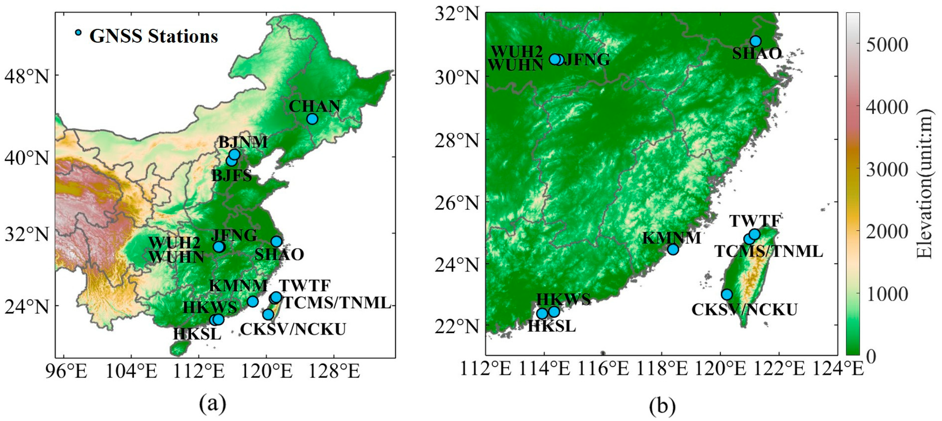
2.1.1. GNSS Data
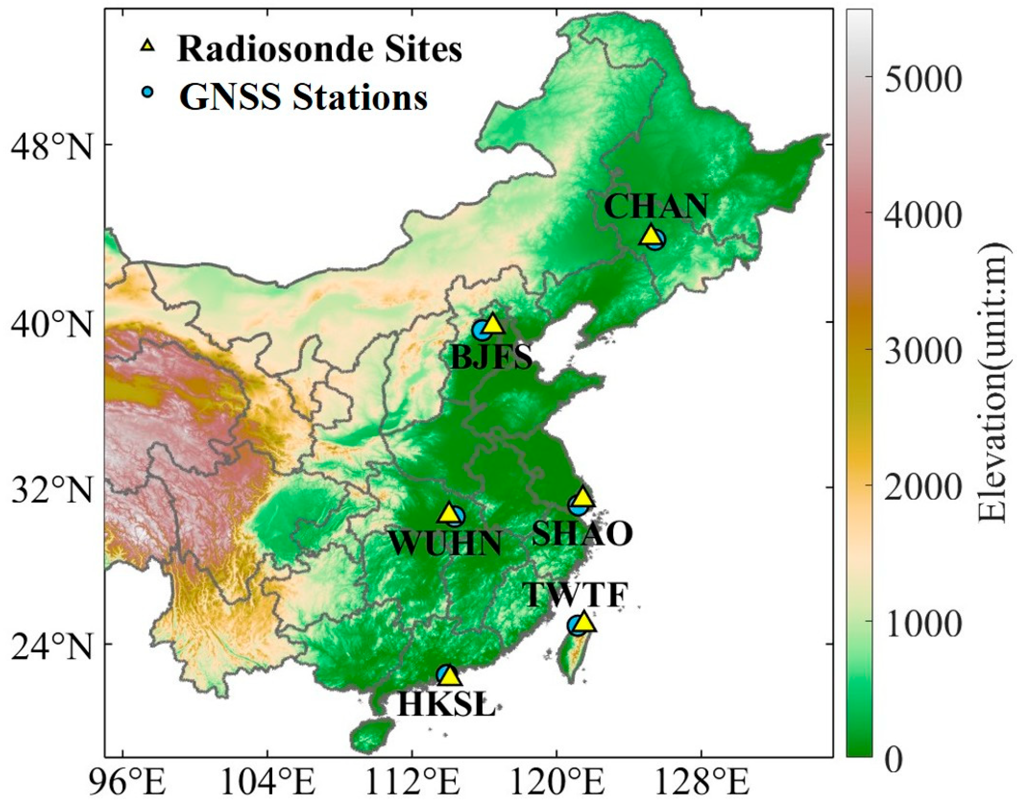
2.1.2. Radiosonde PWV
2.1.3. Temperature
2.2. GNSS PWV Retrieval
2.2.1. GNSS Data Solution Software
2.2.2. GNSS PWV Retrieval Method
2.3. Bayesian Statistics
2.4. Wavelet Transform
2.5. Fast Fourier Transform
2.6. Evaluation Indicators
3. Results and Discussion
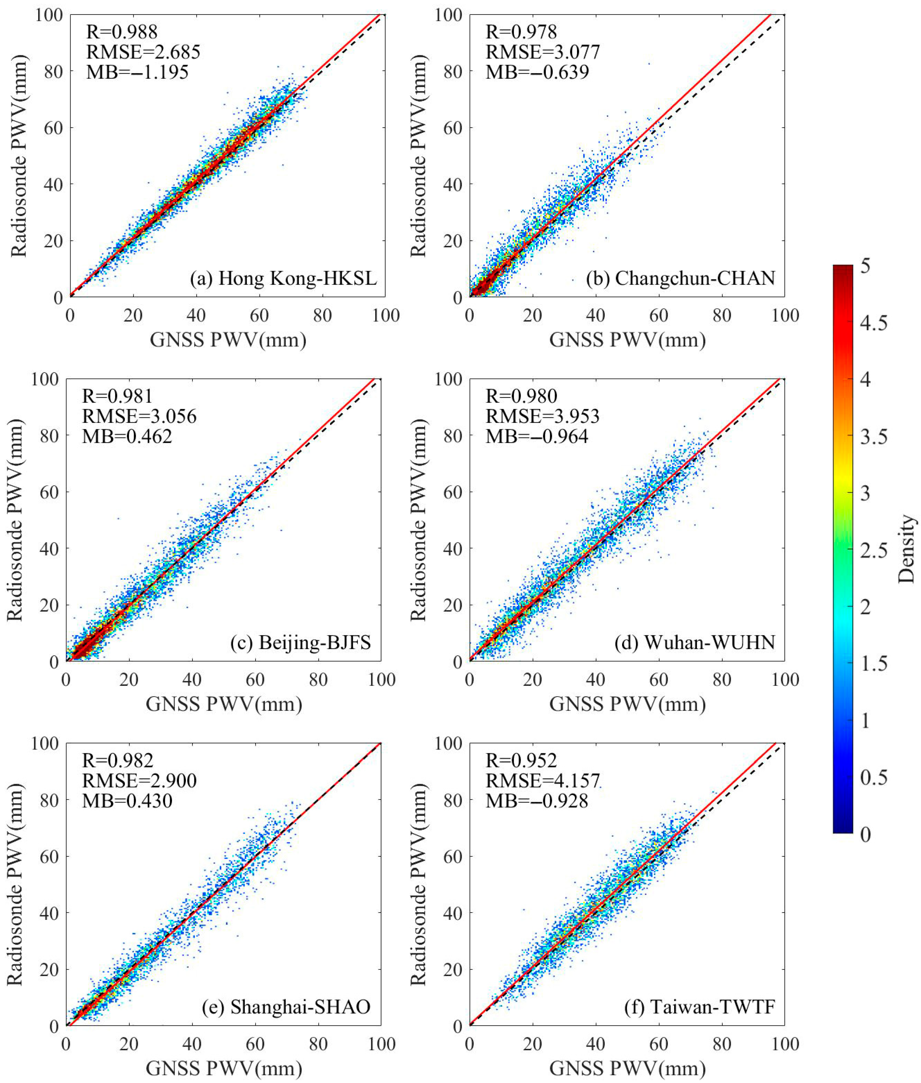
3.1. Accuracy Assessment of GNSS PWV
3.2. Spatial and Temporal Variations in GNSS PWV
3.2.1. Overall Characteristics of PWV in the Time Domain
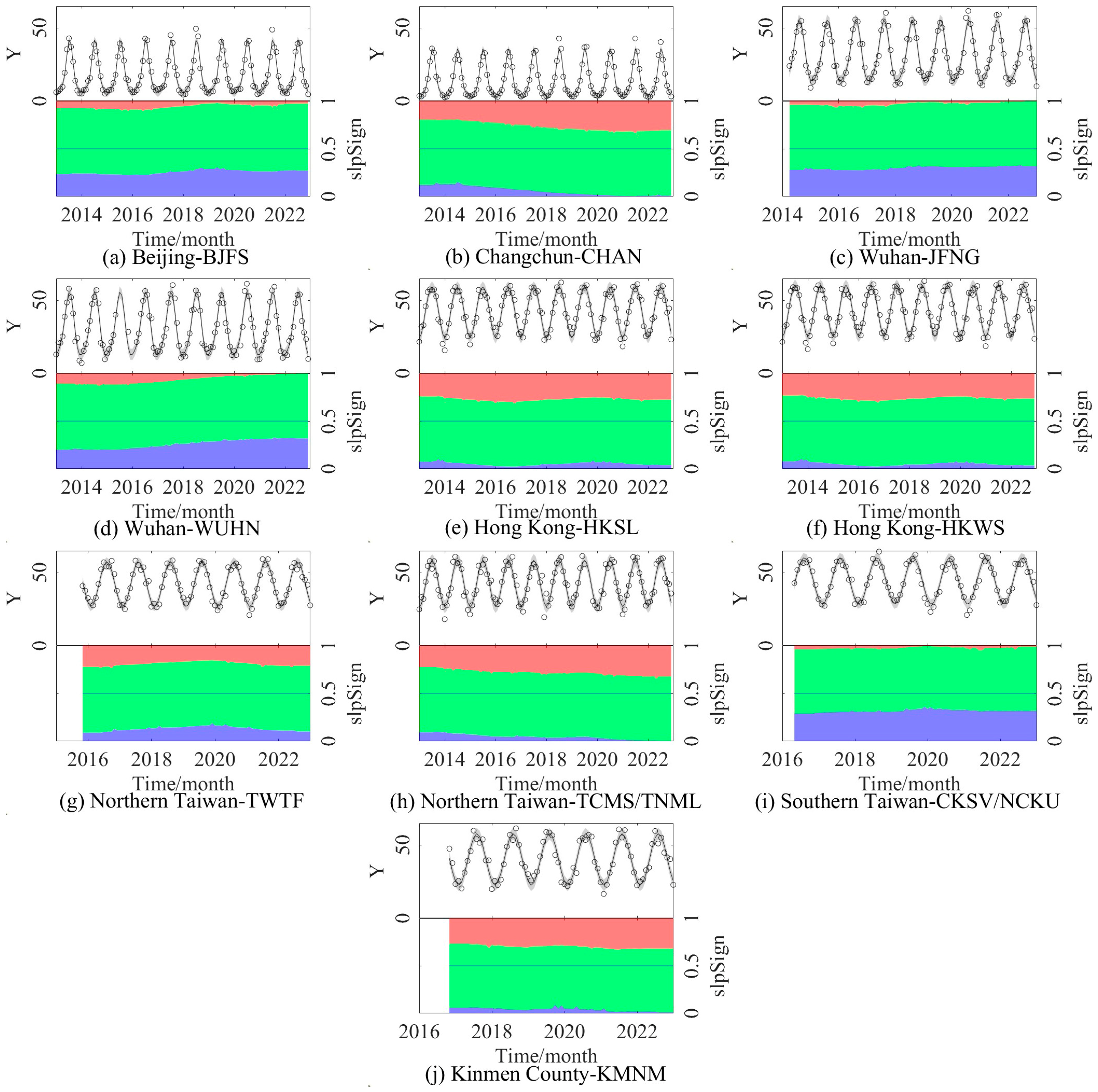
3.2.2. Trend Variations in PWV Time Series
3.3. Frequency-Domain Characterization of GNSS PWV
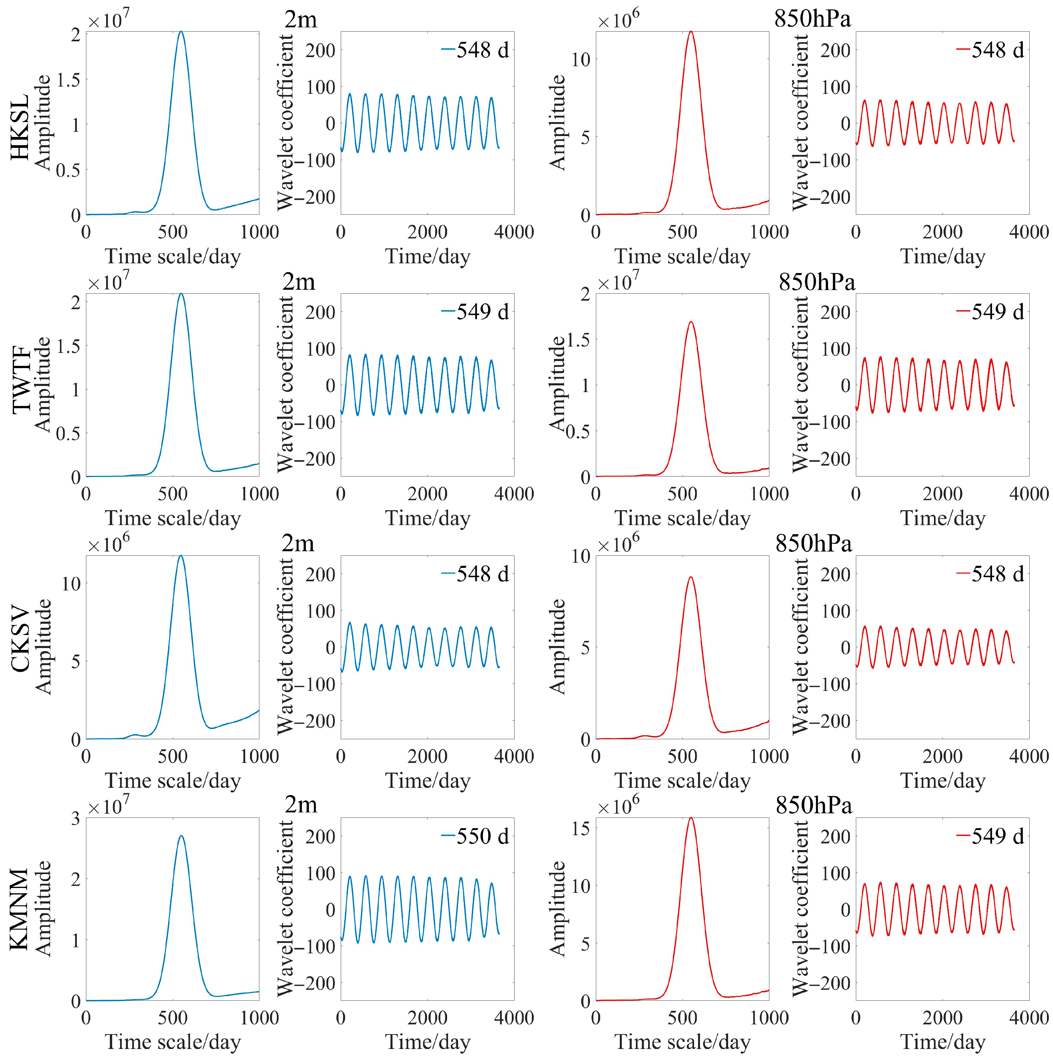
3.3.1. Annual/Semi-Annual Period of GNSS PWV
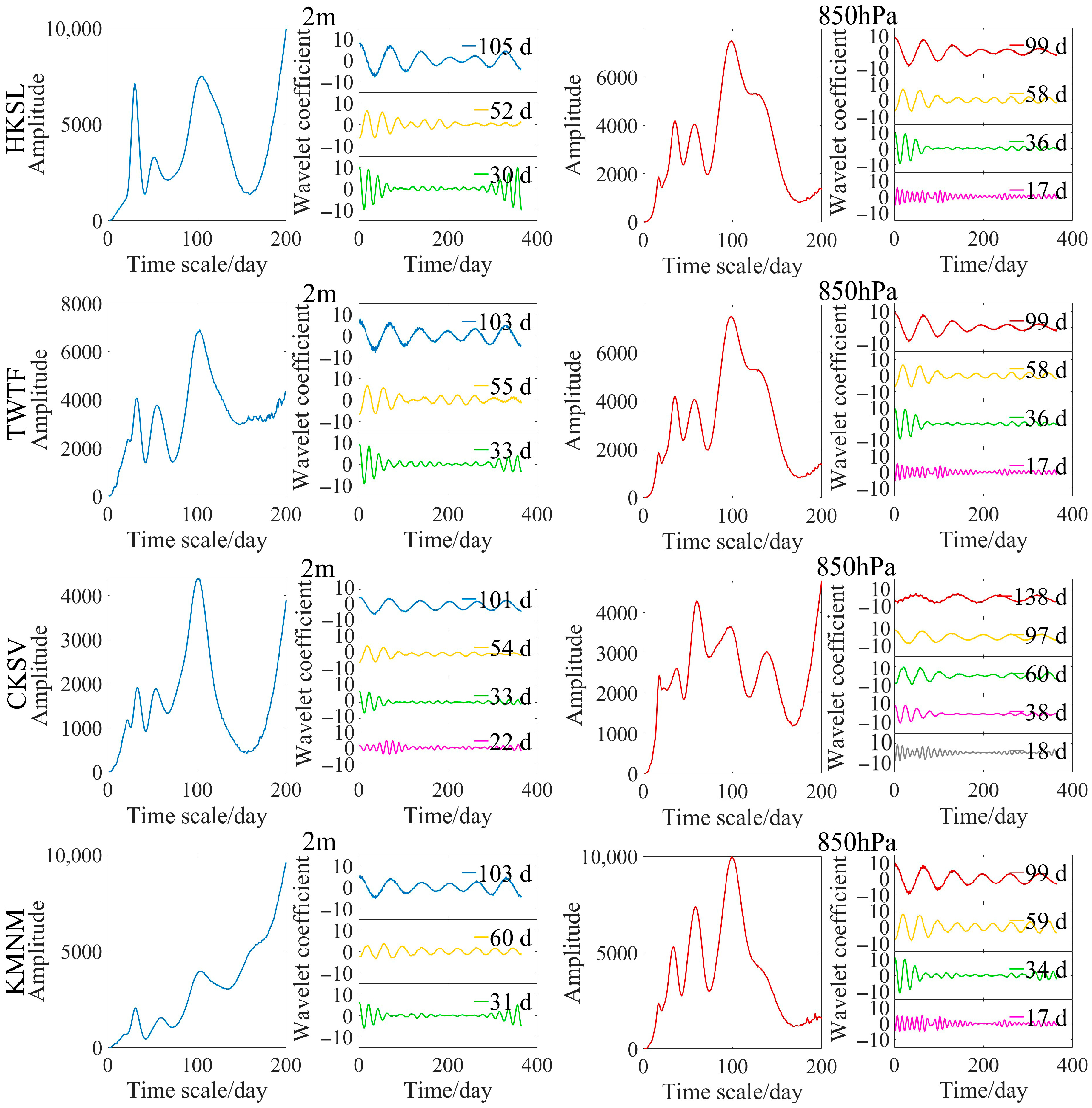
3.3.2. Seasonal/Monthly Fluctuation Period of GNSS PWV
3.4. Short-Time Frequency-Domain Characterizations of GNSS PWV
3.5. The Effect of Atmospheric Temperature on PWV
4. Limitations and Prospects
5. Conclusions
Author Contributions
Funding
Institutional Review Board Statement
Informed Consent Statement
Data Availability Statement
Acknowledgments
Conflicts of Interest
Abbreviations
| PWV | Precipitable Water Vapor |
| GNSS | Global Navigation Satellite System |
| IGS | International GNSS Service |
| FFT | Fast Fourier Transform |
| ERA5 | ECMWF Reanalysis v5 |
| ZHD | Zenith Hydrostatic Delay |
| ZTD | Zenith Tropospheric Delay |
| ZWD | Zenith Wet Delay |
References
- Charlesworth, E.; Plöger, F.; Birner, T.; Baikhadzhaev, R.; Abalos, M.; Abraham, N.L.; Akiyoshi, H.; Bekki, S.; Dennison, F.; Jöckel, P.; et al. Stratospheric water vapor affecting atmospheric circulation. Nat. Commun. 2023, 14, 3925. [Google Scholar] [CrossRef] [PubMed]
- Zhu, H.; Chen, K.; Hu, S.; Liu, J.; Shi, H.; Wei, G.; Chai, H.; Li, J.; Wang, T. Using the Global Navigation Satellite System and Precipitation Data to Establish the Propagation Characteristics of Meteorological and Hydrological Drought in Yunnan, China. Water Resour. Res. 2023, 59, e2022WR033126. [Google Scholar] [CrossRef]
- Zhang, J.; Chen, H.; Fang, X.; Yin, Z.; Hu, R. Warming-induced hydrothermal anomaly over the Earth’s three Poles amplifies concurrent extremes in 2022. NPJ Clim. Atmos. Sci. 2024, 7, 8. [Google Scholar] [CrossRef]
- Zhou, X.; Li, Y.; Xiao, C.; Chen, W.; Mei, M.; Wang, G. High-impact Extreme Weather and Climate Events in China: Summer 2024 Overview. Adv. Atmos. Sci. 2025, 42, 1064–1076. [Google Scholar] [CrossRef]
- Liu, X.; Wang, Y.; Huang, J.; Yu, T.; Jiang, N.; Yang, J.; Zhan, W. Assessment and calibration of FY-4A AGRI total precipitable water products based on CMONOC. Atmos. Res. 2022, 271, 106096. [Google Scholar] [CrossRef]
- Jiang, P.; Liu, R.; Huo, Y.; Wu, Y.; Ye, S.; Wang, S.; Mu, X.; Zhu, L. Retrieving the Atmospheric Water Vapor Profile Combining FY-4A/GIIRS and Ground-Based GNSS PWV in Hong Kong Region. IEEE Trans. Geosci. Remote Sens. 2025, 63, 1–9. [Google Scholar] [CrossRef]
- Wang, J.; Liu, Z. Improving GNSS PPP accuracy through WVR PWV augmentation. J. Geod. 2019, 93, 1685–1705. [Google Scholar] [CrossRef]
- Sun, Q.; Vihma, T.; Jonassen, M.O.; Zhang, Z. Impact of Assimilation of Radiosonde and UAV Observations from the Southern Ocean in the Polar WRF Model. Adv. Atmos. Sci. 2020, 37, 441–454. [Google Scholar] [CrossRef]
- Dessler, A.E.; Davis, S.M. Trends in tropospheric humidity from reanalysis systems. J. Geophys. Res.-Atmos. 2010, 115, D19127. [Google Scholar] [CrossRef]
- Li, W.; Yao, Y.; Zhang, L.; Peng, W.; Du, Z.; Zuo, Y.; Wang, W. Evaluating global precipitable water vapor products from four public reanalysis using radiosonde data. J. Geod. Geodyn. 2025, in press. [Google Scholar] [CrossRef]
- Mo, Z.; Zeng, Z.; Huang, L.; Liu, L.; Huang, L.; Zhou, L.; Ren, C.; He, H. Investigation of Antarctic Precipitable Water Vapor Variability and Trend from 18 Year (2001 to 2018) Data of Four Reanalyses Based on Radiosonde and GNSS Observations. Remote Sens. 2021, 13, 3901. [Google Scholar] [CrossRef]
- Ssenyunzi, R.C.; Oruru, B.; D’ujanga, F.M.; Realini, E.; Barindelli, S.; Tagliaferro, G.; von Engeln, A.; van de Giesen, N. Performance of ERA5 data in retrieving Precipitable Water Vapour over East African tropical region. Adv. Space Res. 2020, 65, 1877–1893. [Google Scholar] [CrossRef]
- Wang, S.; Xu, T.; Nie, W.; Jiang, C.; Yang, Y.; Fang, Z.; Li, M.; Zhang, Z. Evaluation of Precipitable Water Vapor from Five Reanalysis Products with Ground-Based GNSS Observations. Remote Sens. 2020, 12, 1817. [Google Scholar] [CrossRef]
- Zhao, T.; Fu, C.; Ke, Z.; Guo, W. Global Atmosphere Reanalysis Datasets: Current Status and Recent Advances. Adv. Earth Sci. 2010, 25, 241–254. [Google Scholar]
- Bevis, M.; Businger, S.; Herring, T.A.; Rocken, C.; Anthes, R.A.; Ware, R.H. GPS meteorology: Remote sensing of atmospheric water vapor using the global positioning system. J. Geophys. Res.-Atmos. 1992, 97, 15787–15801. [Google Scholar] [CrossRef]
- Dong, C.; Yu, F.; Zhang, W.; Fang, L.; Wei, K.; Lou, Y.; Ou, S. An Improved Rainfall Forecasting Method with GNSS-PWV Three Factor Threshold. Geomat. Inf. Sci. Wuhan Univ. 2025, 50, 866–873. [Google Scholar] [CrossRef]
- Wang, Z.; Chai, H.; Zheng, N.; Ming, L.; Chen, P. Research on filling missing GNSS precipitable water vapor time series data using the PSORF model combined with reanalysis datasets. Meas. Sci. Technol. 2025, 36, 016014. [Google Scholar] [CrossRef]
- Borger, C.; Beirle, S.; Wagner, T. Analysis of global trends of total column water vapour from multiple years of OMI observations. Atmos. Chem. Phys. 2022, 22, 10603–10621. [Google Scholar] [CrossRef]
- Kim, S.; Sharma, A.; Wasko, C.; Nathan, R. Linking Total Precipitable Water to Precipitation Extremes Globally. Earth Future 2022, 10, e2021EF002473. [Google Scholar] [CrossRef]
- Parracho, A.C.; Bock, O.; Bastin, S. Global IWV trends and variability in atmospheric reanalyses and GPS observations. Atmos. Chem. Phys. 2018, 18, 16213–16237. [Google Scholar] [CrossRef]
- Wan, N.; Lin, X.; Pielke, R.A., Sr.; Zeng, X.; Nelson, A.M. Global total precipitable water variations and trends over the period 1958–2021. Hydrol. Earth Syst. Sci. 2024, 28, 2123–2137. [Google Scholar] [CrossRef]
- Foster, J.; Bevis, M.; Raymond, W. Precipitable water and the lognormal distribution. J. Geophys. Res.-Atmos. 2006, 111, D15102. [Google Scholar] [CrossRef]
- Liu, Y.; Zhang, B.; Yao, Y.; Zhao, Q.; Xu, C.; Yan, X.; Zhang, L. Revealing the spatiotemporal patterns of water vapor and its link to North Atlantic Oscillation over Greenland using GPS and ERA5 data. Sci. Total Environ. 2024, 918, 170596. [Google Scholar] [CrossRef] [PubMed]
- Khutorova, O.G.; Khutorov, V.E.; Teptin, G.M. Tropospheric Water Vapor Long-term Periodicities and ENSO Relation in European Territory of Russia. Earth Space Sci. 2019, 6, 2480–2486. [Google Scholar] [CrossRef]
- Jadala, N.B.; Sridhar, M.; Dashora, N.; Dutta, G. Annual, seasonal and diurnal variations of integrated water vapor using GPS observations over Hyderabad, a tropical station. Adv. Space Res. 2020, 65, 529–540. [Google Scholar] [CrossRef]
- Liu, Y.; Wang, Y.; Ding, K.; Liu, X.; Zhan, W. Short Term Frequency Domain Characteristics of GNSS PWV Based on CMONOC. J. Geod. Geodyn. 2021, 41, 1118–1122. [Google Scholar]
- Yang, F.; Gong, X.; Li, Z.; Wang, Y.; Song, S.; Wang, H.; Chen, R. Spatiotemporal distribution and impact factors of GNSS-PWV in China based on climate region. Adv. Space Res. 2024, 73, 4187–4201. [Google Scholar] [CrossRef]
- Wang, F.; Liu, C.; Xu, Y. Analyzing Population Density Disparity in China with GIS-automated Regionalization: The Hu Line Revisited. Chin. Geogr. Sci. 2019, 29, 541–552. [Google Scholar] [CrossRef]
- Pielke, R., Jr.; Burgess, M.G.; Ritchie, J. Plausible 2005–2050 emissions scenarios project between 2 °C and 3 °C of warming by 2100. Environ. Res. Lett. 2022, 17, 024027. [Google Scholar] [CrossRef]
- Ferreira, A.P.; Gimeno, L. Determining precipitable water vapour from upper-air temperature, pressure and geopotential height. Q. J. R. Meteorol. Soc. 2024, 150, 484–522. [Google Scholar] [CrossRef]
- Gong, S.; Fiifi Hagan, D.; Lu, J.; Wang, G. Validation on MERSI/FY-3A precipitable water vapor product. Adv. Space Res. 2018, 61, 413–425. [Google Scholar] [CrossRef]
- Liu, H.; Tang, S.; Zhang, S.; Hu, J. Evaluation of MODIS water vapour products over China using radiosonde data. Int. J. Remote Sens. 2015, 36, 680–690. [Google Scholar] [CrossRef]
- Hersbach, H.; Bell, B.; Berrisford, P.; Hirahara, S.; Horányi, A.; Muñoz-Sabater, J.; Nicolas, J.; Peubey, C.; Radu, R.; Schepers, D.; et al. The ERA5 global reanalysis. Q. J. R. Meteorol. Soc. 2020, 146, 1999–2049. [Google Scholar] [CrossRef]
- Glaser, S.; Fritsche, M.; Sośnica, K.; Rodríguez-Solano, C.J.; Wang, K.; Dach, R.; Hugentobler, U.; Rothacher, M.; Dietrich, R. A consistent combination of GNSS and SLR with minimum constraints. J. Geod. 2015, 89, 1165–1180. [Google Scholar] [CrossRef]
- Geng, J.; Wen, Q.; Zhang, Q.; Li, G.; Zhang, K. GNSS observable-specific phase biases for all-frequency PPP ambiguity resolution. J. Geod. 2022, 96, 11. [Google Scholar] [CrossRef]
- Geng, J.; Zhang, Q.; Li, G.; Liu, J.; Liu, D. Observable-specific phase biases of Wuhan multi-GNSS experiment analysis center’s rapid satellite products. Satell. Navig. 2022, 3, 23. [Google Scholar] [CrossRef]
- Zeng, J.; Geng, J.; Li, G.; Tang, W. Improving cycle slip detection in ambiguity-fixed precise point positioning for kinematic LEO orbit determination. GPS Solut. 2024, 28, 135. [Google Scholar] [CrossRef]
- Li, X.; Han, X.; Li, X.; Liu, G.; Feng, G.; Wang, B.; Zheng, H. GREAT-UPD: An open-source software for uncalibrated phase delay estimation based on multi-GNSS and multi-frequency observations. GPS Solut. 2021, 25, 66. [Google Scholar] [CrossRef]
- Li, X.; Yuan, L.; Li, X.; Huang, J.; Shen, Z.; Tan, Y. GREAT-PVT: An open-source software for multi-frequency and multi-GNSS PPP-AR and RTK. GPS Solut. 2025, 29, 157. [Google Scholar] [CrossRef]
- Li, X.; Zheng, H.; Li, X.; Yuan, Y.; Wu, J.; Han, X. Open-source software for multi-GNSS inter-frequency clock bias estimation. GPS Solut. 2023, 27, 84. [Google Scholar] [CrossRef]
- Xie, S.; Zhang, P.; Wang, X. Influence of Dynamic Mapping Functions on GPS Baseline Quality. J. Geod. Geodyn. 2017, 37, 192–195. [Google Scholar]
- Saastamoinen, J. Atmospheric Correction for the Troposphere and Stratosphere in Radio Ranging Satellites. In The Use of Artificial Satellites for Geodesy; American Geophysical Union: Washington, DC, USA, 1972; Volume 15, pp. 247–251. [Google Scholar]
- Bevis, M.; Businger, S.; Chiswell, S.; Herring, T.A.; Anthes, R.A.; Rocken, C.; Ware, R.H. GPS Meteorology: Mapping Zenith Wet Delays onto Precipitable Water. J. Appl. Meteorol. Climatol. 1994, 33, 379–386. [Google Scholar] [CrossRef]
- Boehm, J.; Heinkelmann, R.; Schuh, H. Short Note: A global model of pressure and temperature for geodetic applications. J. Geod. 2007, 81, 679–683. [Google Scholar] [CrossRef]
- Sun, J.; Fan, S.; Zang, J.; Zhou, C.; Liu, Y. Accuracy comparison and analysis for three GPT models. Sci. Surv. Mapp. 2018, 43, 63–67,75. [Google Scholar]
- Zhou, T.; Popescu, S.C.; Lawing, A.M.; Eriksson, M.; Strimbu, B.M.; Bürkner, P.C. Bayesian and Classical Machine Learning Methods: A Comparison for Tree Species Classification with LiDAR Waveform Signatures. Remote Sens. 2017, 10, 39. [Google Scholar] [CrossRef]
- Zhao, K.; Valle, D.; Popescu, S.; Zhang, X.; Mallick, B. Hyperspectral remote sensing of plant biochemistry using Bayesian model averaging with variable and band selection. Remote Sens. Environ. 2013, 132, 102–119. [Google Scholar] [CrossRef]
- Li, J.; Li, Z.-L.; Wu, H.; You, N. Trend, seasonality, and abrupt change detection method for land surface temperature time-series analysis: Evaluation and improvement. Remote Sens. Environ. 2022, 280, 113222. [Google Scholar] [CrossRef]
- Zhao, K.; Wulder, M.A.; Hu, T.; Bright, R.; Wu, Q.; Qin, H.; Li, Y.; Toman, E.; Mallick, B.; Zhang, X.; et al. Detecting change-point, trend, and seasonality in satellite time series data to track abrupt changes and nonlinear dynamics: A Bayesian ensemble algorithm. Remote Sens. Environ. 2019, 232, 111181. [Google Scholar] [CrossRef]
- White, J.H.R.; Walsh, J.E.; Thoman, R.L., Jr. Using Bayesian statistics to detect trends in Alaskan precipitation. Int. J. Climatol. 2021, 41, 2045–2059. [Google Scholar] [CrossRef]
- Morlet, J.; Arens, G.; Fourgeau, E.; Giard, D. Wave propagation and sampling theory; Part I, Complex signal and scattering in multilayered media. Geophysics 1982, 47, 203–221. [Google Scholar] [CrossRef]
- Morlet, J.; Arens, G.; Fourgeau, E.; Giard, D. Wave propagation and sampling theory; Part II, Sampling theory and complex waves. Geophysics 1982, 47, 222–236. [Google Scholar] [CrossRef]
- Li, L.; Song, Y.; Zhou, J.L. Preliminary Exploration of GNSS Meteorological Elements Using Wavelet Transform for Rainstorm Prediction. J. Geod. Geodyn. 2020, 40, 225–230. [Google Scholar]
- Wang, Y.; Liu, B.; Liu, Y. Correlation Analysis of GPS PWV and Meteorological Elements Based on Wavelet Transform. J. Geod. Geodyn. 2017, 37, 721–725. [Google Scholar]
- Grossmann, A.; Morlet, J. Decomposition of Hardy Functions into Square Integrable Wavelets of Constant Shape. SIAM J. Math. Anal. 1984, 15, 723–736. [Google Scholar] [CrossRef]
- Kumar, P.; Foufoula-Georgiou, E. Wavelet analysis for geophysical applications. Rev. Geophys. 1997, 35, 385–412. [Google Scholar] [CrossRef]
- Cooley, J.W.; Tukey, J.W. An Algorithm for the Machine Calculation of Complex Fourier Series. Math. Comput. 1965, 19, 297–301. [Google Scholar] [CrossRef]
- Shi, H.; Zhang, R.; Nie, Z.; Li, Y.; Chen, Z.; Wang, T. Research on variety characteristics of mainland China troposphere based on CMONOC. J. Geod. Geodyn. 2018, 9, 411–417. [Google Scholar] [CrossRef]
- Wang, J.; Zhang, L. Climate applications of a global, 2-hourly atmospheric precipitable water dataset derived from IGS tropospheric products. J. Geod. 2009, 83, 209–217. [Google Scholar] [CrossRef]
- Zhao, Q.; Yao, Y.; Yao, W.; Zhang, S. GNSS-derived PWV and comparison with radiosonde and ECMWF ERA-Interim data over mainland China. J. Atmos. Sol.-Terr. Phys. 2019, 182, 85–92. [Google Scholar] [CrossRef]
- Zhao, Y.; Zhou, S.; Wang, S.; Sun, J.; San, X. The Error Analysis for the Remote Sensing of Water Vapor Data by Ground Based GPS in Tengchong, Yunnan Province. J. Geosci. Environ. Prot. 2019, 7, 231–245. [Google Scholar] [CrossRef]
- Shangguan, S.; Lin, H.; Wei, Y.; Tang, C. Spatiotemporal Modes Characteristics and SARIMA Prediction of Total Column Water Vapor over China during 2002–2022 Based on AIRS Dataset. Atmosphere 2022, 13, 885. [Google Scholar] [CrossRef]
- Wu, M.; Jin, S.; Li, Z.; Cao, Y.; Ping, F.; Tang, X. High-Precision GNSS PWV and Its Variation Characteristics in China Based on Individual Station Meteorological Data. Remote Sens. 2021, 13, 1296. [Google Scholar] [CrossRef]
- Zhang, J.; Zhao, T.; Dai, A.; Zhang, W. Detection and Attribution of Atmospheric Precipitable Water Changes since the 1970s over China. Sci. Rep. 2019, 9, 17609. [Google Scholar] [CrossRef] [PubMed]
- Willett, K.M.; Gillett, N.P.; Jones, P.D.; Thorne, P.W. Attribution of observed surface humidity changes to human influence. Nature 2007, 449, 710–712. [Google Scholar] [CrossRef] [PubMed]
- Luo, Z.; Liu, J.; Zhang, Y.; Zhou, J.; Yu, Y.; Jia, R. Spatiotemporal characteristics of urban dry/wet islands in China following rapid urbanization. J. Hydrol. 2021, 601, 126618. [Google Scholar] [CrossRef]
- Liu, S. Assessment of Regional Climate Effects of Urbanization around Subtropical City Wuhan in Summer Using Numerical Modeling. Atmosphere 2024, 15, 185. [Google Scholar] [CrossRef]
- Li, X.; Fan, W.; Wang, L.; Luo, M.; Yao, R.; Wang, S.; Wang, L. Effect of urban expansion on atmospheric humidity in Beijing-Tianjin-Hebei urban agglomeration. Sci. Total Environ. 2021, 759, 144305. [Google Scholar] [CrossRef] [PubMed]
- Luan, Q.; Cao, Q.; Huang, L.; Liu, Y.; Wang, F. Identification of the Urban Dry Islands Effect in Beijing: Evidence from Satellite and Ground Observations. Remote Sens. 2022, 14, 809. [Google Scholar] [CrossRef]
- Chen, Y.; Zhang, Y.; Tian, J.; Tang, Z.; Wang, L.; Yang, X. Understanding the Propagation of Meteorological Drought to Groundwater Drought: A Case Study of the North China Plain. Water 2024, 16, 501. [Google Scholar] [CrossRef]
- Liu, Q.; Zhang, X.; Xu, Y.; Li, C.; Zhang, X.; Wang, X. Characteristics of groundwater drought and its correlation with meteorological and agricultural drought over the North China Plain based on GRACE. Ecol. Indic. 2024, 161, 111925. [Google Scholar] [CrossRef]
- Sprenger, M.; Leistert, H.; Gimbel, K.; Weiler, M. Illuminating hydrological processes at the soil-vegetation-atmosphere interface with water stable isotopes. Rev. Geophys. 2016, 54, 674–704. [Google Scholar] [CrossRef]
- Trenberth, K.E.; Fasullo, J.; Smith, L. Trends and variability in column-integrated atmospheric water vapor. Clim. Dyn. 2005, 24, 741–758. [Google Scholar] [CrossRef]
- Dong, B.; Dai, A. The influence of the Interdecadal Pacific Oscillation on Temperature and Precipitation over the Globe. Clim. Dyn. 2015, 45, 2667–2681. [Google Scholar] [CrossRef]
- Feng, L.; Zhang, R.-H.; Yu, B.; Han, X. Roles of Wind Stress and Subsurface Cold Water in the Second-Year Cooling of the 2017/18 La Niña Event. Adv. Atmos. Sci. 2020, 37, 847–860. [Google Scholar] [CrossRef]
- Sherwood, S.C.; Roca, R.; Weckwerth, T.M.; Andronova, N.G. Tropospheric water vapor, convection, and climate. Rev. Geophys. 2010, 48, RG2001. [Google Scholar] [CrossRef]
- Nakamura, M.; Miyama, T. Impacts of the Oyashio Temperature Front on the Regional Climate. J. Clim. 2014, 27, 7861–7873. [Google Scholar] [CrossRef]
- Xie, Y.; Wei, F.; Chen, G.; Zhang, T.; Hu, L. Analysis of the 2008 heavy snowfall over South China using GPS PWV measurements from the Tibetan Plateau. Ann. Geophys. 2010, 28, 1369–1376. [Google Scholar] [CrossRef]
- Kim, Y.-J.; Jee, J.-B.; Lim, B. Investigating the Influence of Water Vapor on Heavy Rainfall Events in the Southern Korean Peninsula. Remote Sens. 2023, 15, 340. [Google Scholar] [CrossRef]
- Wang, X.; Zhang, Q.; Zhang, S. Periodic Oscillation Analysis of GPS Water Vapor Time Series Using Combined Algorithm Based on EMD and WD. Geomat. Inf. Sci. Wuhan Univ. 2018, 43, 620–628. [Google Scholar] [CrossRef]
- O’Gorman, P.A.; Muller, C.J. How closely do changes in surface and column water vapor follow Clausius–Clapeyron scaling in climate change simulations? Environ. Res. Lett. 2010, 5, 025207. [Google Scholar] [CrossRef]
- Shi, P.; Sun, S.; Wang, M.; Li, N.; Wang, J.A.; Jin, Y.; Gu, X.; Yin, W. Climate change regionalization in China (1961–2010). Sci. China Earth Sci. 2014, 57, 2676–2689. [Google Scholar] [CrossRef]
- Xian, T.; Su, K.; Zhang, J.; Hu, H.; Wang, H. Precipitable Water Vapor Retrieval Based on GNSS Data and Its Application in Extreme Rainfall. Remote Sens. 2025, 17, 2301. [Google Scholar] [CrossRef]
- Zhao, Q.; Liu, Y.; Yao, W.; Yao, Y. Hourly Rainfall Forecast Model Using Supervised Learning Algorithm. IEEE Trans. Geosci. Remote Sens. 2022, 60, 1–9. [Google Scholar] [CrossRef]


| Stations | Areas | Temporal Coverage | Data Points Before Exclusion | Data Points After Exclusion |
|---|---|---|---|---|
| BJFS | Beijing | 2013-01-01–2022-12-31 | 83,926 | 83,829 |
| BJNM | Beijing | 2013-01-01–2020-07-08 | 53,865 | 53,772 |
| CHAN | Changchun | 2013-01-01–2022-12-31 | 83,544 | 82,914 |
| CKSV | Southern Taiwan | 2016-10-16–2022-12-31 | 50,900 | 50,900 |
| HKSL | Hong Kong | 2013-01-01–2022-12-31 | 85,189 | 85,189 |
| HKWS | Hong Kong | 2013-01-01–2022-12-31 | 85,280 | 85,280 |
| JFNG | Wuhan | 2014-03-26–2022-12-31 | 75,026 | 75,024 |
| KMNM | Kinmen County | 2016-10-16–2022-12-31 | 50,681 | 50,681 |
| NCKU | Southern Taiwan | 2016-04-05–2022-05-19 | 47,560 | 47,560 |
| SHAO | Shanghai | 2013-01-01–2021-07-08 | 44,489 | 44,479 |
| TCMS | Northern Taiwan | 2013-01-01–2021-04-24 | 48,595 | 48,595 |
| TNML | Northern Taiwan | 2013-01-01–2022-12-31 | 45,966 | 45,966 |
| TWTF | Northern Taiwan | 2013-01-01–2022-12-31 | 81,810 | 81,810 |
| WUH2 | Wuhan | 2016-08-31–2022-12-31 | 50,693 | 50,690 |
| WUHN | Wuhan | 2013-01-04–2022-12-31 | 72,874 | 72,867 |
| Processing Key Points | Specific Models and Parameters | |
|---|---|---|
| Double-difference relative positioning | Coordinate parameters | Double-difference network adjustment |
| Receiver clock offset | Differential technique | |
| Observations | Type of observation | GPS observation data |
| Observation periods | 2013-01-01–2022-12-31 | |
| Sampling interval | 30 s | |
| Correction models | Cutoff height angle | 10° |
| Phase entanglement | Correction | |
| Tidal load | Correction of Earth tides, polar tides, and ocean tides | |
| Relativistic effect | Correction | |
| ZTD prior model | VMF1+Saastamoinen | |
| Projection function | °) | |
| Parameter estimation strategies | Satellite orbit | IGS Final Orbital Precision Ephemeris |
| Ambiguity solution | Least-Squares Ambiguity Decorrelation Adjustment | |
| Ambiguity parameter | Floating point solution |
| Stations | First Main Period/d | First Fluctuation Period/d | Second Main Period/d | Second Fluctuation Period/d |
|---|---|---|---|---|
| BJFS | 552 | 363 | 278 | 182 |
| BJNM | 562 | 370 | 286 | 184 |
| CHAN | 552 | 361 | 277 | 183 |
| JFNG | 549 | 365 | 277 | 182 |
| WUH2 | 542 | 368 | 280 | 185 |
| WUHN | 542 | 364 | 281 | 180 |
| SHAO | 611 | 386 | / | / |
| HKSL | 553 | 364 | / | / |
| HKWS | 553 | 364 | / | / |
| KMNM | 544 | 366 | / | / |
| TWTF | 551 | 362 | / | / |
| TCMS | 558 | 366 | / | / |
| TNML | 569 | 365 | / | / |
| CKSV | 542 | 364 | / | / |
| NCKU | 539 | 366 | / | / |
| Stations | Main Period/d | Fluctuation Period/d |
|---|---|---|
| BJFS | 160/43 | 105/31 |
| CHAN | 176/44 | 113/26 |
| JFNG | 94/59/39 | 62/38/25 |
| WUH2 | 97/59/39 | 64/40/26 |
| WUHN | 94/60/39 | 64/40/26 |
| SHAO | 97/60/40 | 56/40/25 |
| HKSL | 184/136/86/41/18 | 121/90/56/27/11 |
| HKWS | 184/136/86/42/18 | 122/92/57/27/12 |
| KMNM | 186/133/91/41/18 | 125/93/58/27/12 |
| TWTF | 132/90/41/18 | 93/58/27/12 |
| CKSV | 194/88/43/18 | 121/56/27/12 |
| NCKU | 184/88/43/18 | 121/56/28/12 |
| Height | BJFS | CHAN | JFNG | SHAO | HKSL | TWTF | CKSV | KMNM |
|---|---|---|---|---|---|---|---|---|
| 2 m | 0.71 | 0.76 | 0.71 | 0.76 | 0.74 | 0.73 | 0.71 | 0.78 |
| 1000 hPa | 0.70 | 0.77 | 0.70 | 0.76 | 0.73 | 0.75 | 0.74 | 0.77 |
| 975 hPa | 0.69 | 0.77 | 0.69 | 0.75 | 0.73 | 0.74 | 0.74 | 0.75 |
| 950 hPa | 0.69 | 0.77 | 0.70 | 0.75 | 0.75 | 0.74 | 0.74 | 0.75 |
| 925 hPa | 0.69 | 0.77 | 0.72 | 0.76 | 0.78 | 0.74 | 0.75 | 0.76 |
| 900 hPa | 0.70 | 0.78 | 0.73 | 0.77 | 0.8 | 0.74 | 0.76 | 0.77 |
| 875 hPa | 0.71 | 0.78 | 0.75 | 0.77 | 0.81 | 0.74 | 0.76 | 0.78 |
| 850 hPa | 0.72 | 0.79 | 0.76 | 0.78 | 0.81 | 0.74 | 0.76 | 0.78 |
| 825 hPa | 0.74 | 0.79 | 0.77 | 0.78 | 0.8 | 0.75 | 0.75 | 0.78 |
| 800 hPa | 0.75 | 0.80 | 0.78 | 0.78 | 0.79 | 0.76 | 0.74 | 0.77 |
| 775 hPa | 0.76 | 0.80 | 0.79 | 0.79 | 0.77 | 0.76 | 0.73 | 0.77 |
| 750 hPa | 0.77 | 0.81 | 0.80 | 0.79 | 0.75 | 0.75 | 0.72 | 0.76 |
| 700 hPa | 0.79 | 0.81 | 0.81 | 0.8 | 0.68 | 0.74 | 0.68 | 0.73 |
| 650 hPa | 0.8 | 0.81 | 0.82 | 0.81 | 0.59 | 0.70 | 0.60 | 0.67 |
| 600 hPa | 0.81 | 0.82 | 0.82 | 0.81 | 0.48 | 0.65 | 0.50 | 0.60 |
Disclaimer/Publisher’s Note: The statements, opinions and data contained in all publications are solely those of the individual author(s) and contributor(s) and not of MDPI and/or the editor(s). MDPI and/or the editor(s) disclaim responsibility for any injury to people or property resulting from any ideas, methods, instructions or products referred to in the content. |
© 2025 by the authors. Licensee MDPI, Basel, Switzerland. This article is an open access article distributed under the terms and conditions of the Creative Commons Attribution (CC BY) license (https://creativecommons.org/licenses/by/4.0/).
Share and Cite
Zhang, T.; Xiong, J.; Hu, S.; Zhao, W.; Huang, M.; Zhang, L.; Xia, Y. Exploring Precipitable Water Vapor (PWV) Variability and Subregional Declines in Eastern China. Sustainability 2025, 17, 6699. https://doi.org/10.3390/su17156699
Zhang T, Xiong J, Hu S, Zhao W, Huang M, Zhang L, Xia Y. Exploring Precipitable Water Vapor (PWV) Variability and Subregional Declines in Eastern China. Sustainability. 2025; 17(15):6699. https://doi.org/10.3390/su17156699
Chicago/Turabian StyleZhang, Taixin, Jiayu Xiong, Shunqiang Hu, Wenjie Zhao, Min Huang, Li Zhang, and Yu Xia. 2025. "Exploring Precipitable Water Vapor (PWV) Variability and Subregional Declines in Eastern China" Sustainability 17, no. 15: 6699. https://doi.org/10.3390/su17156699
APA StyleZhang, T., Xiong, J., Hu, S., Zhao, W., Huang, M., Zhang, L., & Xia, Y. (2025). Exploring Precipitable Water Vapor (PWV) Variability and Subregional Declines in Eastern China. Sustainability, 17(15), 6699. https://doi.org/10.3390/su17156699