Article

Extraction of Basic Features and Typical Operating Conditions of Wind Power Generation for Sustainable Energy Systems

1
The School of Mechanical Engineering, Inner Mongolia University of Science and Technology, Baotou 014010, China
2
Guoneng Hebei Cangdong Power Generation Co., Ltd., Cangzhou 061113, China
*
Author to whom correspondence should be addressed.
Sustainability 2025, 17(14), 6577; https://doi.org/10.3390/su17146577
Submission received: 29 June 2025 / Revised: 16 July 2025 / Accepted: 17 July 2025 / Published: 18 July 2025

Abstract

Accurate extraction of representative operating conditions is crucial for optimizing systems in renewable energy applications. This study proposes a novel framework that combines the Parzen window estimation method, ideal for nonparametric modeling of wind, solar, and load datasets, with a game theory-based time scale selection mechanism. The novelty of this work lies in integrating probabilistic density modeling with multi-indicator evaluation to derive realistic operational profiles. We first validate the superiority of the Parzen window approach over traditional Weibull and Beta distributions in estimating wind and solar probability density functions. In addition, we analyze the influence of key meteorological parameters such as wind direction, temperature, and solar irradiance on energy production. Using three evaluation metrics, the main result shows that a 3-day representative time scale offers optimal accuracy when determined through game theory methods. Validation with real-world data from Inner Mongolia confirms the robustness of the proposed method, yielding low errors in wind, solar, and load profiles. This study contributes a novel 3-day typical profile extraction method validated on real meteorological data, providing a data-driven foundation for optimizing energy storage systems under renewable uncertainty. This framework supports energy sustainability by ensuring realistic modeling under renewable intermittency.

1. Introduction

The increasing reliance on wind and solar energy presents critical challenges to power grid stability due to the inherent intermittency and variability of these resources. A key problem lies in how to effectively characterize and model these fluctuations to guide the design of reliable and economical energy storage systems. The problems of grid integration of wind power and solar power systems stem mainly from their intermittent and fluctuating nature. Fluctuations in wind speed and solar irradiance lead to instability in power generation, which poses a challenge to the stable supply of electricity to the grid. Numerous studies have investigated the role of energy storage systems in addressing the instability caused by the fluctuating outputs of wind and solar power. For example, Yuan et al. [1] and Zhu et al. [2] proposed frameworks that optimize storage capacity in hybrid systems, demonstrating improved power dispatch. Ding et al. [3] and Tong et al. [4] analyzed how declining storage costs and compensation mechanisms can enhance grid reliability. Additionally, Nasser et al. [5] and Ahmed et al. [6] reviewed hybrid hydrogen and photovoltaic (PV) and wind systems, while Lamadrid [7] and Wang et al. [8] emphasized operational complexity under meteorological variability. Together, these works underline the significance of coordinated storage, forecasting, and control strategies—forming the theoretical foundation for this study’s model and optimization design.
In this context—where traditional probability models struggle with multimodal distributions in renewable energy data—the Parzen window estimation method offers a flexible, non-parametric solution.
In the process of extracting representative dataset characteristics of wind power, PV, and electrical load, known functions (such as normal distribution, Beta distribution, and Weibull distribution) fail to accurately describe the probability distribution. Moreover, some classical probability density functions are unimodal, whereas Parzen windows, a non-parametric estimation method, yield probability density functions for wind power, PV, and electrical load sample data that are mostly multimodal, which directly affects the accuracy of the representative day dataset. The paper proposes a method using the Parzen window estimation method and a weighted average method to obtain a representative dataset. As a non-parametric estimation method, the Parzen window estimation does not rely on the constraints of the overall probability distribution and does not overly depend on probability parameters, making the model robust. In summary, although the Beta probability distribution is widely used in various types of data analysis due to its computational simplicity and solid theoretical foundation, the Parzen window method clearly provides a more reasonable and effective probability density estimation for PV data with complex distributional characteristics.
During the selection of representative time scales, different time scales can influence economic optimization, such as inaccurate energy reserve estimates, neglecting long-term trends, failing to consider multiple system operating scenarios, and declining reliability. Therefore, this paper establishes reasonable indicators for representative time scale selection and uses a game theory-based combination weighting method to obtain the most practical representative time scale.
This paper first establishes a Parzen window model and extracts representative dataset characteristics of wind power, PV, and user demand. Then, it develops evaluation indicators for time scale selection, and finally uses the game theory-based combination weighting method to determine the optimal time scale.
The increasing integration of wind and solar energy brings significant uncertainty and intermittency to power systems, which poses serious challenges for load frequency regulation, energy storage sizing, and data-driven dispatch optimization. While many studies have applied machine learning or probabilistic models to characterize renewable outputs, few have focused on extracting representative time scales for multi-source data in a statistically robust way. For certain scenarios, such as: resilient event-triggered MPC for load frequency regulation with wind turbines under false data injection attacks, resilient frequency regulation for microgrids under phasor measurement unit faults and communication intermittency, robust distributed load frequency control for multi-area wind energy-dominated microgrids considering phasor measurement unit failures. However, these works focus primarily on real-time control under cyber-physical disruptions, while less attention has been given to the data preprocessing stage, where representative operating conditions must be selected. In contrast, this paper aims to fill this gap by combining non-parametric statistical modeling with multi-criteria evaluation to determine the optimal typical time scale for hybrid energy systems.
The main contributions of this paper are summarized as follows: A non-parametric Parzen window estimation method is applied to model the probability distributions of wind power, PVoutput, and load demand, which better captures multimodal characteristics compared to traditional Weibull and Beta distributions. Three evaluation indicators are designed to assess the representativeness of different typical time scales (1–7 days) for wind, solar, and load profiles. A combined weighting method based on game theory is developed to determine the optimal typical time scale, considering both subjective (ordinal ranking) and objective (entropy-based) factors. The study validates that the 3-day typical time scale achieves the best overall representativeness for all three energy sources, with minimal deviation from annual average data. The proposed framework provides a foundation for improving data-driven scheduling, energy storage configuration, and renewable integration in power systems. The proposed approach contributes to sustainable energy system modeling by improving representativeness under variability.

2. Literature Review

Renewable energy systems, especially those integrating wind and solar sources, face substantial challenges due to data uncertainty and multimodal distributions. Numerous studies have attempted to characterize these uncertainties using both parametric and non-parametric methods.
A nonparametric framework has been developed for power system security evaluation, employing kernel-based density estimation to model probabilistic distributions of wind power profiles, generation patterns, and electrical load fluctuations [9]. A novel two-stage thresholding method for image segmentation is proposed, integrating weighted Parzen window and linear programming for efficiency [10]. An architecture for multivariate probability density estimation via the Parzen window approach was proposed. It leverages Parzen window methodology to estimate multivariate probability densities, offering a structured framework for such estimations [11]. A two-phase methodology is introduced for region segmentation: initial seed point generation via kernel-based density estimation, followed by logarithmic clustering for boundary identification; iterative region expansion and contour refinement through probabilistic density modeling of spatial distributions [12]. The Parzen window estimation method is employed to extract features from a historical dataset, deriving distributions of representative weekly wind power, solar power, and electrical load. These distributions are compared with Weibull and Beta distributions. A multi-objective optimization framework, combined with evolutionary algorithms, enhances the sizing and allocation of hybrid wind-solar-storage systems to achieve better economic efficiency under dynamic energy market constraints [13]. A stochastic computational framework is developed for power flow uncertainty quantification, employing kernel-based nonparametric methods to derive probabilistic distributions of grid variables while explicitly modeling interdependencies among wind farms, demand profiles, and electric vehicle charging infrastructures [14]. A novel threshold selection framework for image segmentation is developed by integrating information-theoretic metrics with kernel density estimation, enabling adaptive boundary detection in complex visual datasets [15].
A review of wind velocity and wind power prediction methods is presented, focusing on analyzing the characteristics and probability distributions of the wind power dataset, along with the processing of such a dataset by various prediction techniques [16]. A review of dataset preprocessing and mining methods applied to smart meter dataset profiling was conducted, offering novel insights for dataset processing in wind power and PV datasets [17]. A dimensionality-aware scene analysis framework is developed by integrating manifold learning techniques with adaptive density modeling, enabling robust identification of representative patterns in a high-dimensional visual dataset [18]. An intelligent control framework for hybrid solar-wind energy systems is developed, integrating fuzzy inference mechanisms at critical operational nodes to dynamically optimize renewable resource utilization and maximize power conversion efficiency [19]. A description of the seasonal distribution characteristics of PV power generation fluctuations was presented, along with a method for predicting PV power generation uncertainty based on seasonal classification. This approach leverages seasonal patterns to enhance the accuracy of uncertainty predictions in PV power generation [20]. Qadir et al. [21] identified seven key meteorological variables—wind speed, solar irradiance, temperature, humidity, air pressure, wind direction, and cloud cover—as critical determinants of renewable energy output. However, the study did not delve into the individual influence of each parameter. In contrast, our work specifically incorporates wind direction and solar irradiance into the Parzen probability modeling framework, where they shape the distribution curves used for extracting typical profiles. This integration provides a more accurate and context-aware representation of renewable generation. In summary, the current literature highlights the need for integrated frameworks combining accurate probabilistic modeling with representative dataset extraction. This paper aims to address these gaps through a novel methodology grounded in Parzen estimation and game-theory-based time scale optimization.

3. Methods and Analysis

3.1. Parzen Window Estimation Method

The main methods for extracting representative dataset curves are parametric and non-parametric estimation methods. For the uncertainty characteristics of wind/PV, the Parzen window estimation method (a non-parametric estimation method) will be more applicable.
The expression for the Parzen window estimation method is as follows:
f ( x ) = 1 N h i = 1 N K ( x X i h ) ,
To clarify the application of the Parzen window estimation, we provide a brief example. Suppose we observe wind speed samples x1, x2, …, xn from historical data. For a given evaluation point x, the Parzen probability density estimate is obtained by placing a kernel function (e.g., Gaussian) centered at each sample point and computing the average contribution. For instance, let N = 5 and the kernel be Gaussian with bandwidth h = 1.0. Then, the estimated density at x = 8.0 is calculated by averaging the values of the five Gaussian functions evaluated at that point. This process allows us to model complex, multimodal distributions without assuming a predefined parametric form.
In (1), f(x) represents the probability density function; K(x) is the window function; h is the bandwidth (smoothing parameter); N is the total number of samples in the dataset; and Xi is the given sample. Parzen Window functions commonly used in window estimation methods include Gaussian Functions, Triangle functions, and Epanechnikov functions. Their expressions are respectively:
K ( x ) = 1 2 π exp ( 1 2 x 2 ) G a u s s i a n 1   -   x T r i a n g l e 3 4 ( 1   -   x 2 ) E p a n e c h n i k o ,
In (2), The value domain of x in the trigonometric and Epanechnikov functions is 0–1, which needs to be normalised if used for wind velocity/solar radiation and user electrical load estimation. The three window functions have little effect on Parzen window estimation. A major influence on the Parzen window estimation method is the bandwidth h. The effect of different bandwidths on the results for wind velocity, for example, is shown in Figure 1. The bandwidth h is in the interval of [0.01, 10], and the bandwidth with the smallest mean square error is selected as the best bandwidth by matching the optimization in steps of 0.01.
A sensitivity analysis was performed on the kernel bandwidth parameter h, which plays a crucial role in Parzen window estimation. We evaluated the resulting density curves across a range of h values (e.g., 0.1 to 1.0), and observed that overly small or large values of h lead to overfitting or oversmoothing, respectively. This demonstrates the importance of careful selection of h and suggests the necessity of incorporating uncertainty bands when interpreting estimated distributions.

3.2. Extract Typical Data Features

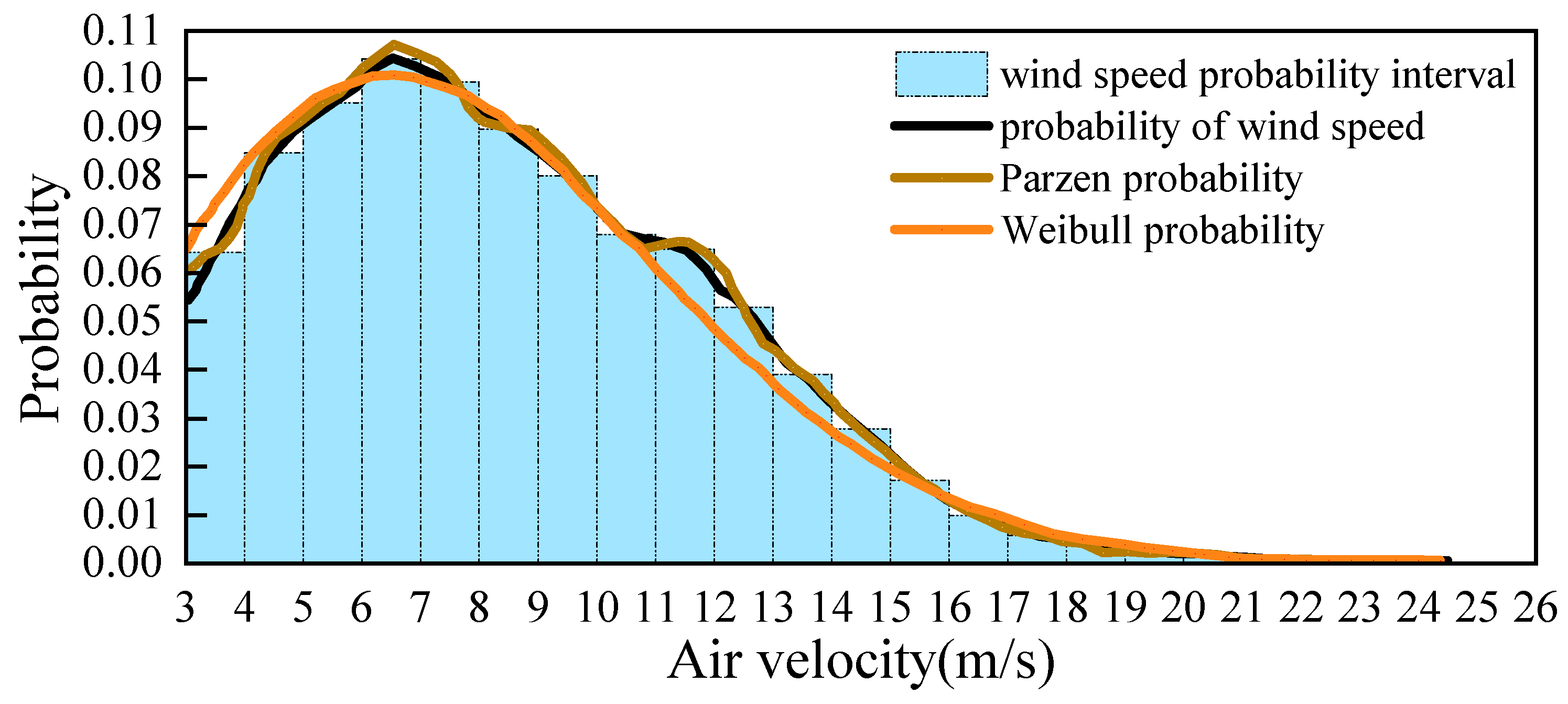
3.2.1. Extraction of Typical Data Features for Wind Power

Extracting representative dataset features for wind power includes three steps: firstly, Wind power generation dataset pretreatment. Removing outliers, filling in missing values, and dataset smoothing to ensure the quality and reliability of the dataset used. Secondly, create a probability density curve. This is done through the Parzen window estimation method, and this method helps to establish the trend of power generation at different wind velocities. Thirdly, verify the theoretical output curve of the turbine. The established wind velocity probability density curves need to be validated against the theoretical power curves of the turbines to assess the accuracy of the model and provide a reference for subsequent work. Through this series of steps, the researcher can establish the representative dataset wind output power curve model, which is of significant value for optimising the design and operation of wind farms. In recent years, machine learning approaches based on meteorological data have been increasingly applied to wind speed forecasting due to their ability to model nonlinear relationships and capture environmental dynamics [22]. These data-driven methods highlight the importance of incorporating diverse meteorological parameters into wind power prediction models.
In this paper, a region in Inner Mongolia Autonomous Region, China, was selected to (N 39°61′, E 109°78′). The actual wind velocity dataset of a weather station from 1 January 2020 to 31 December 2020 was analysed with a sampling interval of fifteen minutes, as shown in Figure 2.
(1) Wind power generation dataset pretreatment
The wind velocity range probability plot is shown in Figure 3. Based on the above dataset characteristics, the Goldwind AW82/1500 wind turbine (Goldwind Science & Technology Co., Ltd., Urumqi, China) is selected, and its parameters are shown in Table 1. As shown in Figure 4, the Goldwind AW82/1500 wind turbine can be used for 92.08% of the total number of working hours, of which 22.92% of the total number of working hours are in full state.
The expression of the Goldwind AW82/1500 wind turbine is:
In (3), v, vr, vcut-in, and vcut-out represent the actual wind velocity, rated wind velocity, cut-in wind velocity, and cut-out wind velocity of the wind turbine, respectively. Pr indicates rated power. The relationship between the dataset is shown in Figure 5, and the red line is the theoretical output power curve of the wind turbine.
P W t t = 0 , v v c u t i n   o r   v v c u t o u t P W r v 3 v c u t i n 3 v r 3 v c u t i n 3 , v c u t i n < v v r P W r , v r < v v c u t i n ,
Taking the representative dataset time selection of 24 h as an example, the modeling process of the Parzen window estimation method for the representative power curve extraction for the minutes 0:00–0:15 is as follows:
(1)
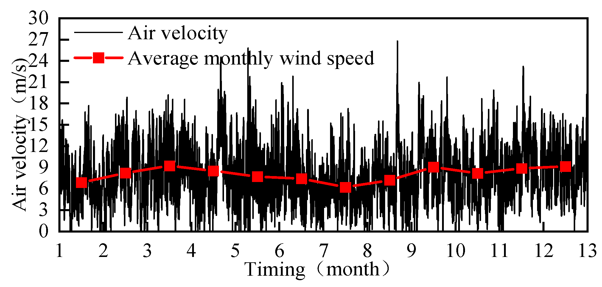
Based on the IEC 61400–12-1 standard [23], valid wind speed measurements from all available days are collected at 1-min intervals during the 0:00–0:15 time period. This yields a sample set of wind speeds {x1, x2, ..., xn} for that time window.
(2)
The sample values are first discretized using a binning method. The wind speed axis is divided into intervals (bins) centered at integer multiples of 0.5 m/s (e.g., 0.5, 1.0, 1.5,...). These bins provide reference points at which the probability density function will be estimated.
(3)
For each bin center x, the Parzen window density estimate f(x) is calculated using a kernel function K and bandwidth h, as defined in Equation (1).
(4)
The resulting density estimates across all bins form a smooth probability distribution curve, representing the wind speed pattern during 0:00–0:15. This curve is then used to identify typical power profiles under varying conditions.
The optimal Weibull probability density distribution curve [24] was obtained using the method described in reference [25]. Figure 6 shows the probability distributions of wind velocities from 0:00 to 0:15 min obtained by different methods. In this time period, the optimal bandwidth is 0.3209, and the optimal shape and scale parameters in the Weibull probability distribution function are 2.1066 and 8.7573, respectively.
To assess the goodness-of-fit of the probability distributions, RMSE and K–S tests were applied following the statistical approach described by Azad et al. [24]. In order to compare the closeness of the Parzen probability, Weibull probability curves to the wind velocity probability, respectively, the following Root Mean Squared Error (RMSE) formula can be used:
R M S E = 1 n i = 1 n y 1 , i y 2 , i 2 ,
In (4), n is the total number of dataset points, y1, i is the ith Standard value, y2, i is the ith value to be compared.
The RMSE values presented in the study quantify the deviation between estimated probability distributions and actual data. Parzen window estimation consistently results in lower RMSE compared to the Weibull and Beta models. The root mean square error was calculated to be 0.001879 for Parzen probability and wind velocity probability and 0.005260 for Weibull probability and wind velocity probability. It is evident that the Parzen method shows superior accuracy in estimating wind speed distributions. The lower RMSE of the Parzen method indicates its ability to capture multimodal distributions more effectively, which is crucial for improving the accuracy of energy output forecasts and the design of energy storage systems. In Figure 6, the Weibull probability distribution differs from the probability histogram, especially at wind velocities between 10 m/s and 15 m/s. The Parzen window estimation method is more in line with the true distribution of the dataset and has a higher degree of accuracy, which provides an initial validation of the reliability of the Parzen probability distribution.
In addition to RMSE, the Kolmogorov–Smirnov (K–S) test was performed to statistically evaluate the goodness-of-fit for different probability models. The K–S test measures the maximum absolute difference between the empirical and estimated cumulative distribution functions (CDFs). Results showed that the Parzen method yielded a K–S statistic of 0.042, significantly lower than that of the Weibull (0.087) distributions. This confirms that the Parzen window approach provides a better fit not only visually but also in terms of statistical agreement with the empirical data. The use of RMSE and K–S jointly strengthens the reliability of the probability modeling results.

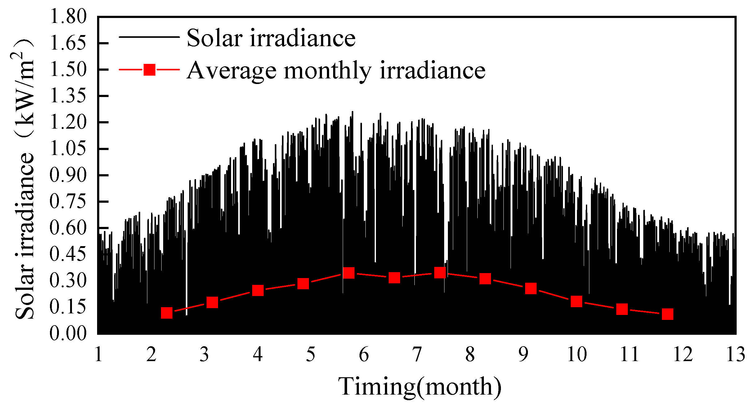
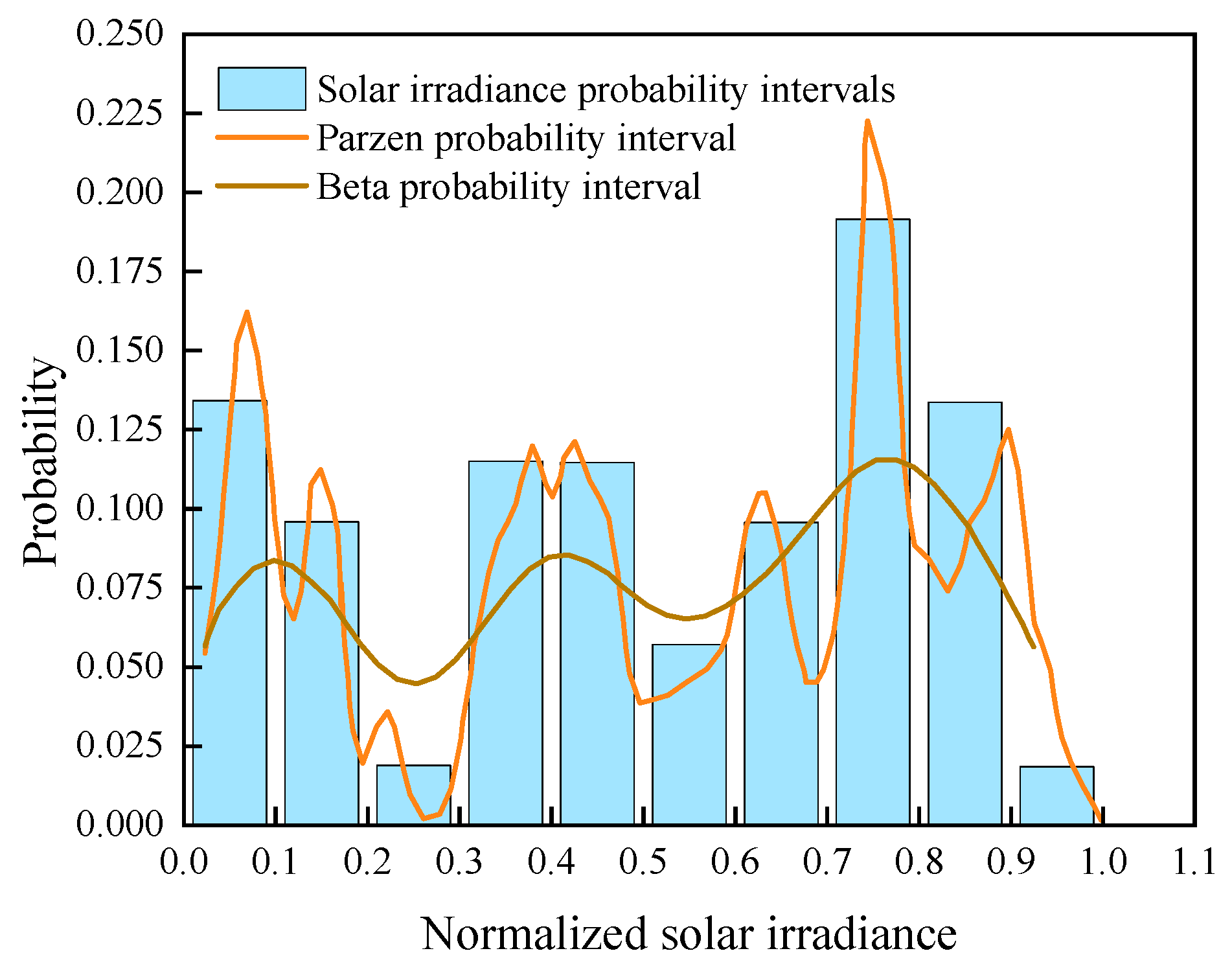
3.2.2. Extracting Typical Data Characteristics of PV

In this paper, the actual solar radiation dataset from a meteorological station in a region of Inner Mongolia Autonomous Region, China (N 39°61′, E 109°78′) from 1 January 2020 to 31 December 2020 is selected for analysis with a sampling interval of fifteen minutes. As shown in Figure 7, the solar radiation observed at the weather station throughout the year is demonstrated.
As shown in Figure 8, 45.91% of the total annual dataset observed by the weather stations had solar radiation equal to 0, and 4.19% had solar radiation greater than 1 KW/m2. Solar irradiance greater than 0 and less than 0.2 KW/m2 accounted for 19.22% of the total. Solar irradiance in the range of 0.2 KW/m2–1 KW/m2 accounted for 30.68% of the total. The annual average solar radiation in the dataset observed at the meteorological stations was 0.23707 KW/m2. But when selecting PV panels, it is not necessary to consider the period of time when the solar radiation is 0. If this situation is not taken into account, the annual average solar radiation is 0.52907 KW/m2.
In a PV power plant, the theoretical expression between solar radiation and the output power of PV power generation is:
In (5), PPV is the output power of the PV plant (in W), I is the solar radiation (in W/m2), A is the area of the PV panel (in m2), ηPPV For the PV panel conversion efficiency, the current domestic mainstream PV panel conversion efficiency between 15–40%, the PV panel conversion efficiency selection of 30%.
P P V t = I t     A     η P V ,
The annual solar radiation is converted into the output power of the PV plant per unit area, and its distribution is shown in Figure 8. The PV panel model CY-TJ 250 is selected, and its parameters are shown in Table 2. According to the above dataset features CY-TJ 250, without counting the moments when the output power is 0, the distribution of the PV panel output power is shown in Figure 9, the PV panel full working hours accounted for 7.75% of the total number of hours, and the output power is less than 100 W h accounted for 51.60% of the total number of hours, which further verifies the scientific nature of the selected PV panel model.
Taking the representative dataset time selection of 24 h as an example, the representative power curve is extracted for the minutes 10:00–10:15, and the modeling process of the Parzen window estimation method is as follows:
(1)
Normalize the dataset and consider the solar radiation exceeding 1000 W/m2 as 1000 W/m2.
(2)
Use Bin’s method to divide the intervals, and use 0.1 W/m2 as an integer multiple of 0.1 W/m2 as the center point, and calculate the probability density of each interval.
(3)
Summarize all the probability densities to build the Parzen window probability distribution curve.
This modeling approach is consistent with methods used in probabilistic forecasting studies such as those described by Shi et al. [20].
The best Beta probability density distribution curve was obtained using the method described in reference [26]. Figure 10 shows the probability distribution of solar radiation for the 10:00–10:15 min obtained by different methods. The optimal bandwidth is 0.0273 for this time period.
When examining the probability distribution characteristics of a PV dataset, Beta distribution curves are often used to model the knowledge accumulation of the dataset. As shown in Figure 10, the shape parameter of the Beta distribution determines the type of distribution it can represent. For complex PV dataset distributions, it is still not possible to accurately capture all the peaks, resulting in its inability to fully reflect the overall distribution trend.
In contrast to the Beta distribution, the Parzen window method provides a nonparametric means of estimating probability densities that makes no assumptions about the form of the distribution of the dataset. A more flexible density estimate is constructed by accumulating weights in the vicinity of sample points through a sliding window. In Figure 10, the root-mean-square error of Parzen probability and wind velocity probability is calculated to be 0.020376, and the root-mean-square error of Weibull probability and wind velocity probability is 0.039799. The Parzen probability distribution is more effective in fitting the PV dataset. This method is not limited by the shape of a particular distribution, and thus can better accommodate the phenomenon of multiple peaks in the dataset, exhibiting a smaller overall error than the Beta distribution.
In summary, although the Beta probability distribution is widely used in various types of dataset analysis due to its computational simplicity and solid theoretical foundation, the Parzen window method clearly provides a more reasonable and effective probability density estimation for the PV dataset with complex distributional characteristics.

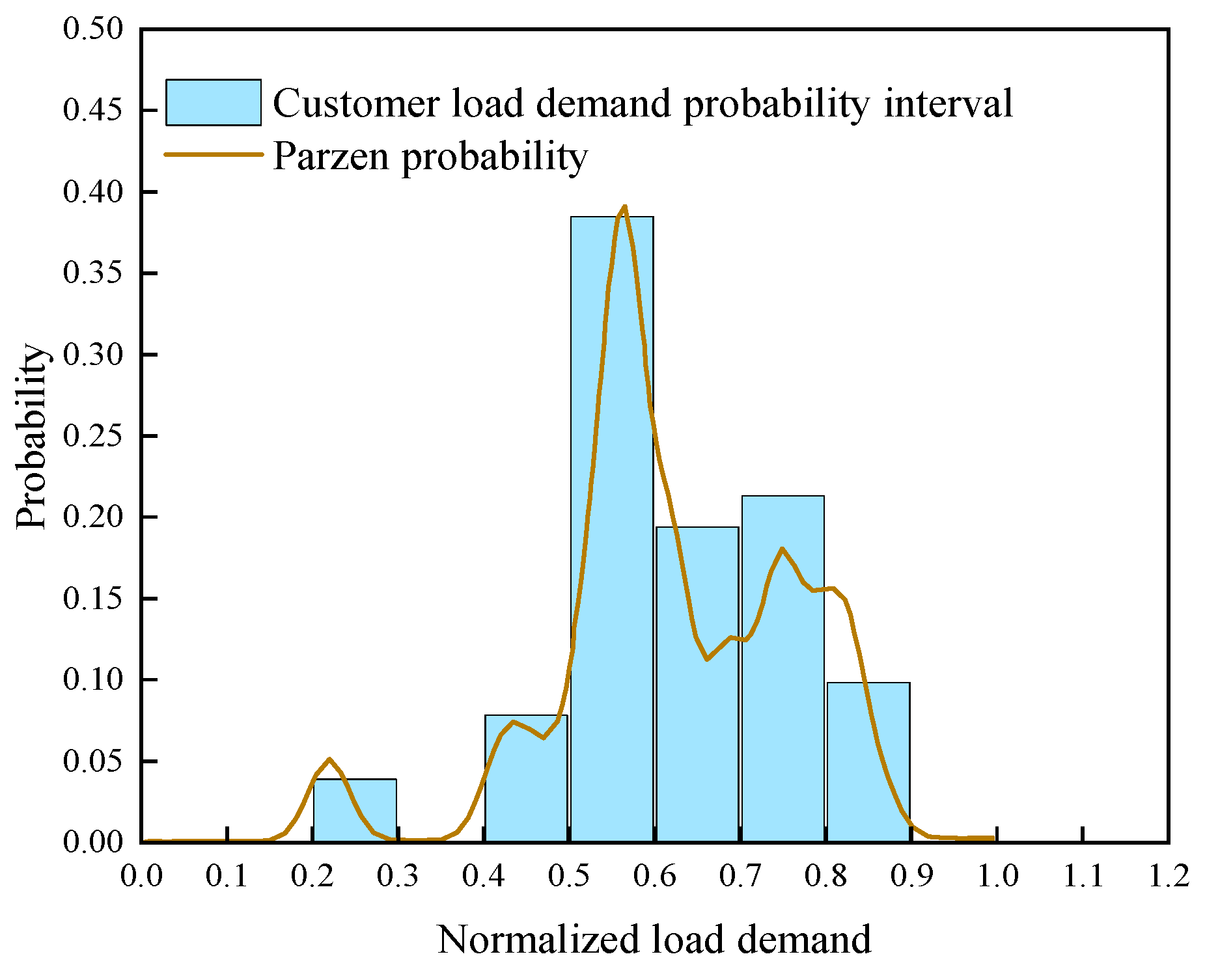
3.2.3. Extract Typical Data Features of User Requirements

In this paper, the actual customer electrical load dataset from 1 January 2020 to 31 December 2020 in a region of Inner Mongolia Autonomous Region of China (N 39°61′, E 109°78′) is selected for analysis, with a sampling interval of fifteen minutes, as shown in Figure 11.
Taking the representative dataset time selection of 24 h as an example, representative power curves were extracted for the minutes 10:00–10:15, and the modeling procedure for the Parzen window estimation method was as follows:
(1)
Normalize the dataset;
(2)
Use Bin’s method to partition the intervals, using an integer multiple of 0.1 MW as the center point, and calculate the probability density of each interval.
(3)
Summarize all probability densities to create a Parzen window probability distribution curve.
Figure 12 shows the probability distribution profile of the customer electrical load demand from 00:00 to 00:15 min obtained using the Parzen window estimation method. The optimal bandwidth is 0.02 during this time period.
Figure 11 shows that there are some seasonal fluctuations in user loads in different months, with the average load being slightly higher in spring and autumn, which may be related to the planned cycle of industrial production or the use of heating and cooling equipment. The load probability distribution for the night time (00:00–00:15) period is shown in Figure 12, and it can be seen that the loads are concentrated in the lower power range, indicating that power usage in this period is dominated by maintenance or base loads, presumably mainly from continuously running equipment such as lighting, servers or a small amount of night-shift production equipment, and less likely to reflect large-scale industrial loads.
To avoid ambiguity in variable interpretation, the symbols used in modeling wind power, solar irradiance, and user load are defined below. The symbols, meanings, units, and typical values are listed in the nomenclature Table 3.

4. Results

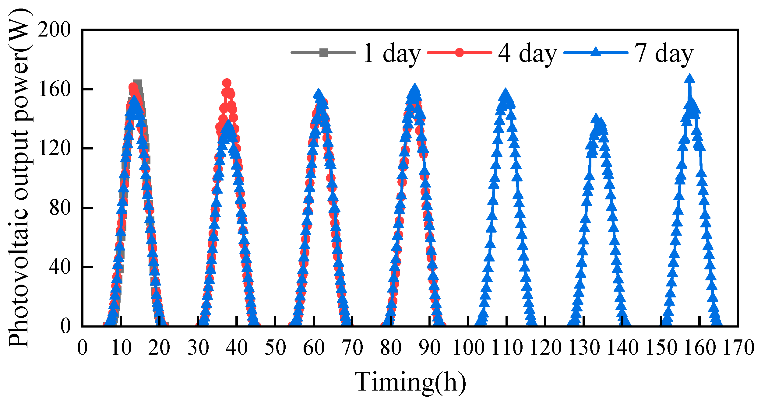
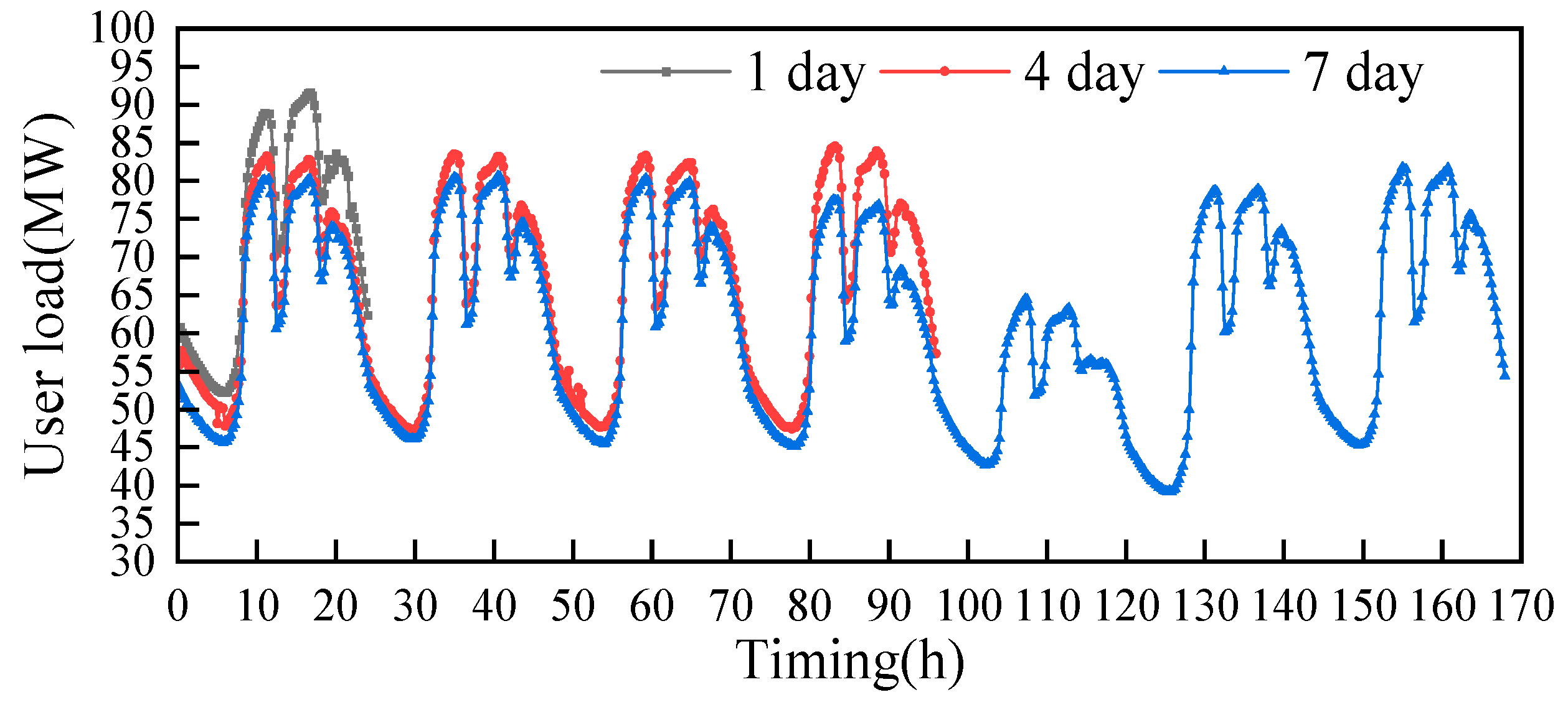
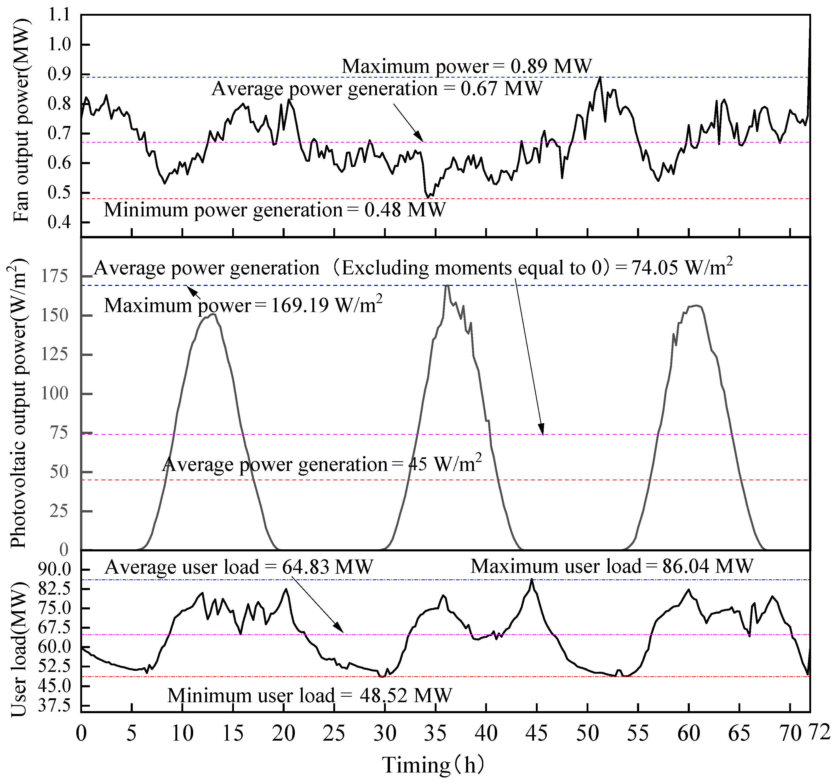
4.1. Typical Time Scale Selection

In addition to probabilistic modeling, the performance of wind and solar power systems is significantly influenced by key environmental parameters. First, wind direction determines the effective wind capture by turbines and affects turbulence, which influences power output stability. Second, solar irradiance is the most direct driver of PV output and is affected by cloud cover, seasonality, and atmospheric conditions. Third, temperature impacts PV efficiency, with higher temperatures reducing energy conversion rates. Fourth, air density—primarily governed by altitude and temperature—affects the kinetic energy of wind and thus the actual wind power output. Lastly, altitude influences both air density and the availability of solar radiation due to atmospheric thinning. By considering these factors, energy prediction models and representative data extraction can be further refined, improving system reliability and accuracy under real-world operating conditions.
In the process of analyzing wind power dataset, PV power generation dataset, and customer electrical load dataset, and extracting representative working conditions, the selection of representative time length is a decisive factor. It directly affects the type of wind, PV, electrical load variation characteristics, and operating conditions that we are able to identify. Furthermore, optimization strategies for wind power prediction in complex terrains, such as mountainous wind farms, underscore the need for precise characterization of representative data profiles [27]. Our study contributes to this by offering a robust framework that integrates probabilistic modeling and time scale evaluation under varied environmental conditions.
As shown in Figure 13, the representative time lengths were selected as 1 day, 4 days, and 7 days, and the representative operating condition curves were obtained for wind power output. Because the cube of wind velocity is proportional to the wind power output, resulting in large differences in the wind power output curves obtained for different representative time lengths, which demonstrates the importance of the representative time length selection.
As shown in Figure 14, representative time lengths of 1 day, 4 days and 7 days were selected and the representative operating conditions curves of the obtained PV outputs were utilized, from which it can be observed that there are large differences in the peak areas of the two representative operating conditions curves (with representative time lengths of 1 day and 7 days) in the interval from 0 to 24 h. In the interval from 24 to 48 h, the two representative operating conditions curves (with representative time lengths of 4 days and 7 days) show a large difference in the peak region, which also proves the importance of the selection of the representative time length.
As shown in Figure 15, the representative time lengths of 1 day, 4 days and 7 days were selected and the representative operating conditions curves of the obtained PV outputs were utilized, from which it can be observed that there are differences in the peak areas of the three representative operating conditions curves in the interval from 0 to 24 h. In particular, there are large differences in the peaks between the operating conditions curves when the representative time length is 1 day and the curves for the other two days. In the interval from 72 to 96 h, both the peak region and the peak-to-valley region of the two representative operating condition curves (with representative time lengths of 4 and 7 days) differed considerably. This also demonstrates the importance of the representative length of time chosen.

4.2. Development of Evaluation Criteria

The purpose of creating statistical indicators is to quantify the difference between a representative day relative to the raw dataset in the aggregate and across time periods. In particular, the deviation of the total electrical load power for the year represents the relative error of the total electrical load power on a representative day, calculated by weighting, to the total electrical load power of the original dataset, as follows [28]:
Δ C 1 = y e a r d C d C y e a r C y e a r ,
In (6), Cd Indicates the sum of representative dataset selected; Cyear Indicates one year of total dataset; year Equals 365; d Indicates the number of days selected. The smaller the deviation of the resource throughout the year, the more accurate the dataset selected for the representative time.
Pearson Correlation Coefficient describes well the correlation of 2 sets of datasets, let there exist 2 arrays of X and Y. When r > 0, then the positive correlation between the 2 sets of datasets is stronger, and when r < 0, then the negative correlation between the 2 sets of datasets is stronger.
r = k = 1 m x k x ̄ y k y ̄ k = 1 m ( x k x ̄ ) 2 k = 1 m ( y k y ̄ ) 2 ,
In (7), m is the number of elements in the array. The average of the absolute values of the correlation coefficients between the representative time dataset and all of the datasets is used as indicator 2, which is calculated as follows:
Δ C 2 = j = 1 y e a r r j y e a r ,
The larger the indicator 2, the stronger the correlation between the representative time dataset and the original dataset, and the better the selection of representative dataset. The dataset bias represents the relative error of the dataset for the same time period over all representative days as compared to the dataset for the same time period of the historical dataset, and indicator 3 is the average of the deviations of the dataset over all time periods, as follows:
Δ C 3 = 1 d 244 t = 1 d 244 i D P i , t i D 0 P i , t i D 0 P i , t ,
In (9), D and D0 are the set of all dates for representative and original dataset, respectively; Pi,t is the dataset value of date d at moment t. The smaller the indicator 3, the better the selection of the representative dataset.
The selection of these three indicators is based on evaluation frameworks proposed in recent power system planning studies [29]. This approach ensures that no single indicator dominates the selection. Strictly in accordance with the above three evaluation indexes, to make a separate evaluation of the representative time length of 1–7 days, the results are shown in Table 4. The optimal representative length of time for all three indicators of wind power is 4 days; the optimal representative length of time for PV indicator 1 is 3 days, and the optimal representative length of time for indicators 2 and 3 is 2 days; the optimal representative length of time for all three indicators of customer electrical load is 3 days. In order to select the optimal representative time length, we need to develop a harmonized weighting scheme.

4.3. Evaluation Methodology

Ordinal Relationship Method [29] (ORA) is a subjective assignment method, with the advantages of a small amount of calculation, without the need to construct a judgment matrix, and its general steps are as follows:
(1) Determine the ordinal relationship of the indicators; based on importance and expert recommendations, establish the ranking order among the three indicators.
(2) The expression of the judgment of the degree of importance between the two neighboring indices is:
R k = X k 1 X k ,
In (10): k takes values of 2 and 3, X represents the value of the evaluation indicator, and Rk denotes the importance between the k-th evaluation indicator and the k-1-th evaluation indicator.
(3) The weight coefficient of the k-th evaluation indicator is:
ω k = 1 + k = 2 3 i = k 3 R i 1 ,
The weight coefficient of the k-1-th evaluation indicator is:
ω k 1 = R k ω k ,
Based on the above process, the subjective weights of the indicators are shown in Table 5. Because in the source-electrical load-storage system the generation side (source) is wind and solar energy, and the electrical load side (electrical load) is the customer electrical load, the electrical load share is 0.5; the share of wind and solar energy is 80 + 20% [13], so the share of wind energy is 0.4 and the share of solar energy is 0.1.
Entropy Weight Method is an objective assignment method [30] with the following general steps:
(1) The dataset Xm × n is quantized with the expression:
X m × n = x 11 x 1 m x n 1 x n m ,
z i j = x i j min x 1 j , , x n j max x 1 j , , x n j min x 1 j , , x n j ,
In (14), zij is the standardized value of the j-th evaluation indicator in the i-th evaluation scheme.
(2) The weight of the j-th evaluation indicator in the i-th evaluation program is:
p i j = z i j i = 1 n z i j ,
(3) The entropy value of the j-th evaluation indicator is:
e j = 1 ln n i = 1 n p i j ln p i j ,
(4) The weight of the j-th evaluation indicator is:
ω j = 1 e j j = 1 m 1 e j ,
Based on the above process, the objective weights of the indicators are shown in Table 6.
The use of game theory methods revolves around the “integration of subjective and objective weights”, the core of which is to coordinate the results of the two weight determination methods through the idea of gaming in order to obtain a more reasonable combination of weights, and thus to solve the problem of the inconsistency of the optimal results of the evaluation indexes in the selection of the typical length of time.
The two sides of the game are the subjective weight W1 obtained by ORA and the objective weight W2 obtained by the Entropy Weight Method [31], whose expressions are (18) and (19):
W 1 = ω 11 , ω 12 ,   ,   ω 1 m T ,
W 2 = ω 21 , ω 22 ,   ,   ω 2 m T ,
The combination weight expression is:
W 12 = ω 11 ω 21 ω 1 m ω 2 m λ 1 λ 2 ,
In (20), λ is the linear combination coefficient. With the sum of the minimum deviations between the combined weights and the individual weights as the objective function, the optimal linear combination coefficient is solved, and its constraint condition expression is:
Min W 12 W 1 2 + W 12 W 2 2 = min λ 1 W 1 + λ 2 W 2 W 1 2 + λ 1 W 1 + λ 2 W 2 W 2 2 ,
In (21): λ1 and λ2 are both greater than or equal to 0, and their sum equals 1. From the principle of differentiation, the model is also required to satisfy the first-order derivative condition, which is expressed as:
λ 1 W 1 W 1 T + λ 2 W 1 W 2 T = W 1 W 1 T λ 1 W 2 W 1 T + λ 2 W 2 W 2 T = W 2 W 2 T ,
Normalizing λ yields the optimal linear combination coefficients, which are expressed as:
λ 1 , O S = λ 1 λ 1 + λ 2 λ 2 , O S = λ 2 λ 1 + λ 2 ,
The expression for the optimal combination of weights for the evaluation indicators is:
W O S = λ 1 , O S W 1 + λ 2 , O S W 2
In summary, the optimal linear scaling factors are found to be 0.3854 and 0.6146 respectively. The final combination weights are obtained by calculation as shown in Table 7.
It was obtained that the representative time length choice of 3 days best characterized the original dataset and had the best overall correlation with the original dataset. The representative dataset feature extraction method is strictly implemented to obtain the representative operating condition curves of wind power, PV, and customer electrical loads, as shown in Figure 16.
From the figure, it can be observed that the average wind power generation is 0.67 MW. At this power level, the wind velocity is 8.48 m/s, which is only 0.23 m/s higher than the actual annual average wind velocity, with an error of 2.7%. This indirectly demonstrates the feasibility of selecting a representative wind power dataset. Ignoring the moments when the power generation is 0, the average PV power generation is 74.05 W/m2. At this power level, the solar radiation is 246.83 W/m2, which is only 9.76 W/m2 higher than the actual annual average solar radiation, with an error of 3.94%. This indirectly demonstrates the feasibility of selecting a representative PV dataset. The average user’s electrical load power is 64.83 MW, which is only 2.24 MW higher than the actual annual average electricity load, with an error of 3.45%. This indirectly demonstrates the feasibility of selecting a representative user electrical load dataset.

4.4. Implications for Grid Operators: A Practical Perspective

The identification of a 3-day typical time scale offers practical value for grid operators. With typical data closely approximating annual averages, these profiles can be directly integrated into daily and seasonal planning of energy dispatch and storage sizing. Similar effects of typical time scale selection on system optimization have been reported in studies involving mountainous wind farms [27] and distributed grids.
For instance, in the Inner Mongolia case study, scheduling energy storage based on typical 3-day curves enables operators to reduce the need for large safety margins in reserve capacity. This reduces the overdesign of battery capacity and allows better planning of generation-load balance under uncertainty. Moreover, typical time-scale-based forecasts can support demand response strategies, allowing more accurate peak-load predictions.
In summary, the proposed methodology provides grid operators with statistically representative data to enhance system planning, improve forecasting models, and optimize energy dispatch strategies.

5. Discussion

The findings of this study confirm the effectiveness of the Parzen window estimation method in capturing the multimodal characteristics inherent in wind, solar, and load datasets. The lower RMSE and K–S statistics compared to Weibull and Beta distributions validate the superiority of the Parzen method for modeling complex renewable energy profiles.
This paper analyzes the uncertainty of wind power generation, solar power generation, and user electrical load variations. Through comparative analysis, when dealing with the uncertainty of wind power generation and user electrical load under representative operating conditions, the Parzen window estimation method (a non-parametric estimation method) is more consistent with the true distribution of the dataset and offers higher accuracy during the process of extracting probability distribution curves. Since the output curves differ significantly when the representative time lengths are set to 1 day, 4 days, and 7 days, the best indicator weight is finally calculated, and it is determined that the representative operating condition curve most closely aligns with the actual situation when the representative time scale is 3 days.
Moreover, the framework’s use of multi-criteria indicators and a game theory-based weighting method provides a more holistic approach to typical day selection. Unlike conventional single-metric approaches, our method ensures that no individual metric disproportionately influences the result, leading to more balanced and representative profiles.

6. Conclusions

While the proposed framework offers a practical tool for typical time scale selection, it also presents certain limitations. The framework has not been verified in real-time scheduling scenarios. The main innovation lies in combining non-parametric density estimation with multi-criteria evaluation for typical day extraction in renewable energy planning. This enhances the representativeness of simulation data used in energy storage sizing, scheduling, and forecasting models. In future research, we plan to extend the method to include other forms of renewable energy (e.g., biomass or hydro) and validate the framework under real-time dispatch scenarios. This method supports the long-term sustainability of renewable-integrated grids by enhancing data-driven planning and energy storage sizing. Recent studies have further highlighted the importance of integrating smart multiphysics approaches in wind turbine design to enhance sustainable performance in Industry 5.0 contexts [32]. Overall, this study contributes a novel, statistically grounded methodology for representative data extraction, with significant implications for grid stability, energy storage sizing, and forecasting accuracy.

Author Contributions

Validation, G.S.; Investigation, Q.Y.; Resources, Q.Y.; Data curation, X.W. and S.G.; Writing—original draft, Y.S. All authors have read and agreed to the published version of the manuscript.

Funding

The research work presented in this paper was financially supported by the Natural Science Foundation of Inner Mongolia (Grant No. 2024QN05042), the First-Class Discipline Scientific Research Project (Grant No. YLXKZX-NKD-039), and the Basic Scientific Research Fund for Universities Directly Under the Administration of the Inner Mongolia Autonomous Region (Grant No. 2024QNJS070).

Institutional Review Board Statement

Not applicable.

Informed Consent Statement

Not applicable.

Data Availability Statement

Data are contained within the article.

Conflicts of Interest

Author Shengyu Gao was employed by Guoneng Hebei Cangdong Power Generation Co., Ltd. The remaining authors declare that the research was conducted in the absence of any commercial or financial relationships that could be construed as a potential conflict of interest.

References

  1. Tiejiang, Y.; Yong, C.; Yiqian, S.; Long, Z.; Shengwei, M. Optimized proportion of energy storage capacity in wind-storage system based on timing simulation and GA algorithm. High Volt. Eng. 2017, 43, 2122–2130. [Google Scholar]
  2. Zhu, R.; Zhao, A.L.; Wang, G.C.; Xia, X.; Yang, Y. An Energy Storage Performance Improvement Model for Grid-Connected Wind-Solar Hybrid Energy Storage System. Comput. Intell. Neurosci. 2020, 2020, 8887227. [Google Scholar] [CrossRef] [PubMed]
  3. Ding, Z.; Bu, W.; Xu, R.; Feng, S. Application of Energy Storage Technology in Photovoltaic Power Generation System. In Proceedings of the 8th International Conference on Management and Computer Science (ICMCS 2018), Shenyang, China, 10–12 August 2018; Atlantis Press: Dordrecht, The Netherlands, 2018; pp. 463–466. [Google Scholar]
  4. Tong, F.; Yuan, M.; Lewis, N.S.; Davis, S.J.; Caldeira, K. Effects of deep reductions in energy storage costs on highly reliable wind and solar electricity systems. iScience 2020, 23, 101484. [Google Scholar] [CrossRef] [PubMed]
  5. Nasser, M.; Megahed, T.F.; Ookawara, S.; Hassan, H. A review of water electrolysis–based systems for hydrogen production using hybrid/solar/wind energy systems. Environ. Sci. Pollut. Res. 2022, 29, 86994–87018. [Google Scholar] [CrossRef] [PubMed]
  6. Ahmed, M.M.R.; Mirsaeidi, S.; Koondhar, M.A.; Karami, N.; Tag-Eldin, E.M.; Ghamry, N.A.; El-Sehiemy, R.A.; Alaas, Z.M.; Sharaf, A.M. Mitigating Uncertainty Problems of Renewable Energy Resources Through Efficient Integration of Hybrid Solar PV/Wind Systems into Power Networks. IEEE Access 2024, 12, 30311–30328. [Google Scholar] [CrossRef]
  7. Lamadrid, A.J. Optimal use of energy storage systems with renewable energy sources. Int. J. Electr. Power Energy Syst. 2015, 71, 101–111. [Google Scholar] [CrossRef]
  8. Wang, F.; Zhen, Z.; Mi, Z.; Sun, H.; Su, S.; Yang, G. Solar irradiance feature extraction and support vector machines based weather status pattern recognition model for short-term photovoltaic power forecasting. Energy Build. 2015, 86, 427–438. [Google Scholar] [CrossRef]
  9. Ul Hassan, R.; Yan, J.; Liu, Y. Security risk assessment of wind integrated power system using Parzen window density estimation. Electr. Eng. 2022, 104, 1997–2008. [Google Scholar] [CrossRef]
  10. Xiong, F.; Zhang, Z.; Ling, Y.; Zhang, J. Image thresholding segmentation based on weighted Parzen-window and linear programming techniques. Sci. Rep. 2022, 12, 13635. [Google Scholar] [CrossRef] [PubMed]
  11. Stanković, D.; Draganić, A.; Lekić, N.; Ioana, C.; Orović, I. An architecture for Parzen-based multivariate probability density estimation. In Proceedings of the 2024 32nd Telecommunications Forum (TELFOR), Belgrade, Serbia, 26–27 November 2024; IEEE: New York, NY, USA, 2024; pp. 1–4. [Google Scholar]
  12. de Souza Rebouças, E.; De Medeiros, F.N.; Marques, R.C.; Chagas, J.V.; Guimarães, M.T.; Santos, L.O.; Medeiros, A.G.; Peixoto, S.A. Level set approach based on Parzen Window and floor of log for edge computing object segmentation in digital images. Appl. Soft Comput. 2021, 105, 107273. [Google Scholar] [CrossRef]
  13. Yu, Q.; Gao, S.; Sun, G.; Qin, R. Optimization of wind and solar energy storage system capacity configuration based on the Parzen window estimation method. J. Renew. Sustain. Energy 2023, 15, 064103. [Google Scholar] [CrossRef]
  14. Rouhani, M.; Mohammadi, M.; Kargarian, A. Parzen window density estimator-based probabilistic power flow with correlated uncertainties. IEEE Trans. Sustain. Energy 2016, 7, 1170–1181. [Google Scholar] [CrossRef]
  15. Xiong, F.; Zhang, J.; Ling, Y.; Zhang, Z. A novel image thresholding method combining entropy with Parzen window estimation. Comput. J. 2022, 65, 2231–2244. [Google Scholar] [CrossRef]
  16. Wang, Y.; Zou, R.; Liu, F.; Zhang, L.; Liu, Q. A review of wind speed and wind power forecasting with deep neural networks. Appl. Energy 2021, 304, 117766. [Google Scholar] [CrossRef]
  17. Dahunsi, F.M.; Olawumi, A.E.; Ale, D.T.; Sarumi, O.A. A systematic review of data pre-processing methods and unsupervised mining methods used in profiling smart meter data. AIMS Electron. Electr. Eng. 2021, 5, 284–314. [Google Scholar] [CrossRef]
  18. Wang, X.; Zhong, F.; Xu, Y.; Liu, X.; Li, Z.; Liu, J.; Zhao, Z. Extraction and Joint Method of PV–Load Typical Scenes Considering Temporal and Spatial Distribution Characteristics. Energies 2023, 16, 6458. [Google Scholar] [CrossRef]
  19. Balakishan, P.; Chidambaram, I.A.; Manikandan, M. Smart fuzzy control based hybrid PV-wind energy generation system. Mater. Today Proc. 2023, 80, 2929–2936. [Google Scholar] [CrossRef]
  20. Shi, M.; Yin, R.; Wang, Y.; Li, D.; Han, Y.; Yin, W. Photovoltaic power interval forecasting method based on kernel density estimation algorithm. IOP Conf. Ser. Earth Environ. Sci. 2020, 615, 012062. [Google Scholar] [CrossRef]
  21. Qadir, Z.; Khan, S.I.; Khalaji, E.; Munawar, H.S.; Al-Turjman, F.; Mahmud, M.P.; Kouzani, A.Z.; Le, K. Predicting the energy output of hybrid PV–wind renewable energy system using feature selection technique for smart grids. Energy Rep. 2021, 7, 8465–8475. [Google Scholar] [CrossRef]
  22. Yetis, Y.; Tehrani, K.; Jamshidi, M. Wind speed forecasting using machine learning approach based on meteorological data-a case study. Energy Environ. Res. 2022, 12, 1–11. [Google Scholar] [CrossRef]
  23. IEC 61400-12-1-2017; Wind Turbines Generator Systems-Part 12-1: Power Performance Measurements of Electricity Producing Wind Turbines. British Standard: London, UK, 2005.
  24. Azad, A.K.; Rasul, M.G.; Alam, M.M.; Uddin, S.A.; Mondal, S.K. Analysis of wind energy conversion system using Weibull distribution. Procedia Eng. 2014, 90, 725–732. [Google Scholar] [CrossRef]
  25. Chen, H.; Li, H.; Xu, Y.; Chen, M.; Wang, L.; Dai, H.; Xu, D.; Tang, X.; Li, X.; Hu, Y.; et al. Research Progress of Energy Storage Technologies in China in 2022. Energy Storage Sci. Technol. 2023, 12, 1516–1552. (In Chinese) [Google Scholar]
  26. Jani, V.; Abdi, H. Optimal allocation of energy storage systems considering wind power uncertainty. J. Energy Storage 2018, 20, 244–253. [Google Scholar] [CrossRef]
  27. He, J.; Zhang, Z. Optimization Study of Wind Power Prediction in Mountainous Wind Farms. In Proceedings of the 2023 3rd International Conference on Energy, Power and Electrical Engineering (EPEE), Wuhan, China, 15–17 September 2023; IEEE: New York, NY, USA, 2023; pp. 150–154. [Google Scholar]
  28. Junxi, T.; Huazhen, C.; Chong, G.; Wu, Z.; Ying, S. A User Load Curve Analysis Method Based on Time Series Data Mining. Power Syst. Prot. Control. 2021, 49, 140–148. (In Chinese) [Google Scholar]
  29. Guohua, F.; Xiaojing, Y.; Huaizhu, Y.; Tao, L.; Ziqi, S. Evaluation of Rural River Ecological Status Based on Fuzzy Matter-element Method. China Rural. Water Hydropower 2022, 4, 80–84. (In Chinese) [Google Scholar]
  30. Shuqiang, Z.; Shanfa, T. Comprehensive Evaluation of Power Transmission Network Planning Schemes Based on Improved Analytic Hierarchy Process, CRITIC Method and Technique for Order Preference by Similarity to an Ideal Solution. Electr. Power Autom. Equip. 2019, 39, 143–148, 162. (In Chinese) [Google Scholar]
  31. Hao, L.I.; Liang, G.A.; Peigen, L.I. Topology optimization of structures under multiple loading cases with a new compliance-volume product. Eng. Optim. 2014, 46, 725–744. [Google Scholar]
  32. Tehrani, K.; Beikbabaei, M.; Mehrizi-Sani, A.; Jamshidi, M. A smart multiphysics approach for wind turbines design in industry 5.0. J. Ind. Inf. Integr. 2024, 42, 100704. [Google Scholar] [CrossRef]
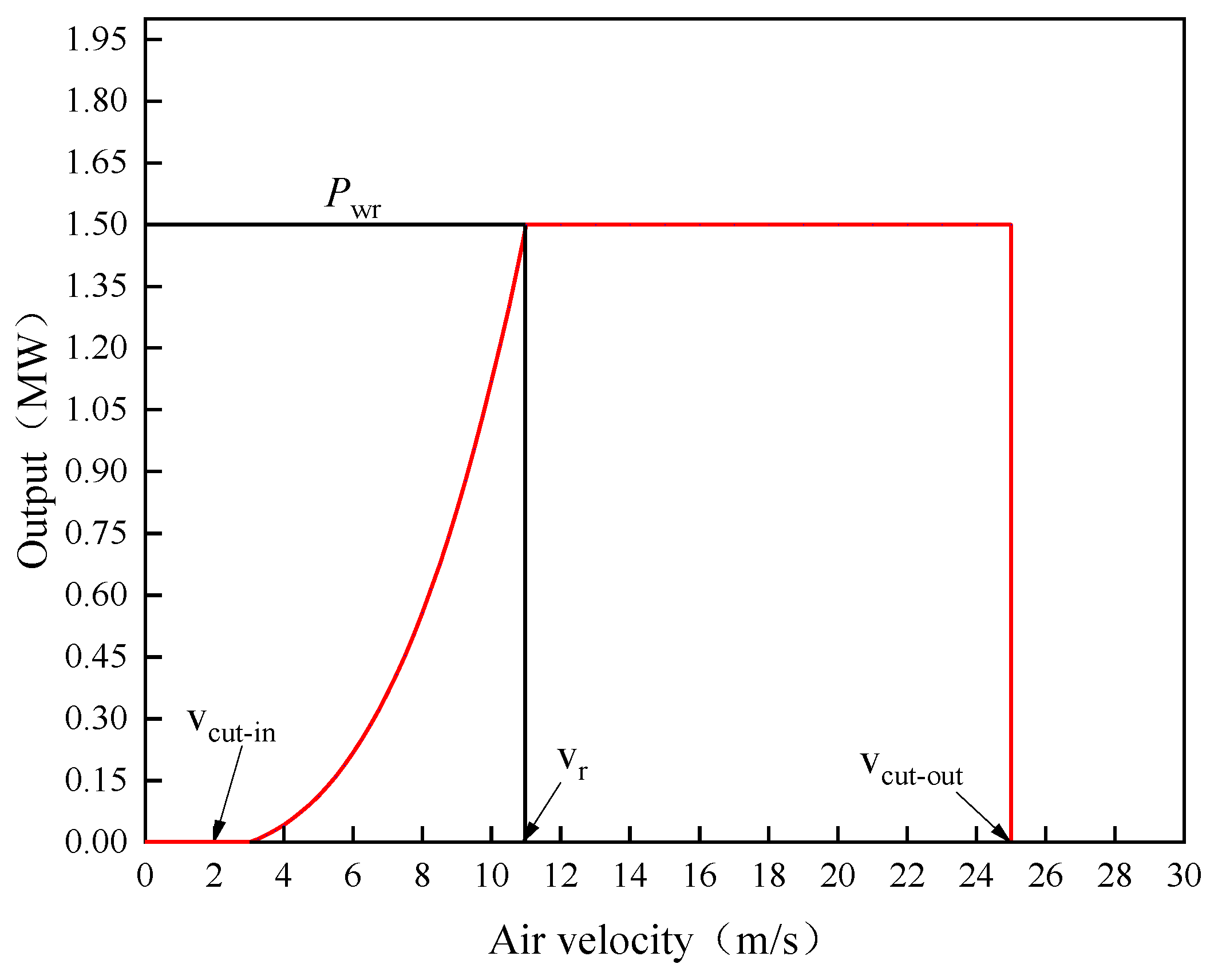
Figure 1. Probability density curves for different bandwidths.
Sustainability 17 06577 g001
Figure 2. Real-time wind velocity at wind farms.
Sustainability 17 06577 g002
Figure 3. Wind speed range histogram.
Sustainability 17 06577 g003
Figure 4. Probability plot of the operating range of the Goldwind AW82/1500 wind turbine.
Sustainability 17 06577 g004
Figure 5. Wind turbine output power curve.
Sustainability 17 06577 g005
Figure 6. Probability plot of wind velocity distribution (00:00–00:15).
Sustainability 17 06577 g006
Figure 7. Real-time solar energy of PV power plants.
Sustainability 17 06577 g007
Figure 8. Probability distribution of solar irradiance under different time scales.
Sustainability 17 06577 g008
Figure 9. Probability plot of the working interval of CY-TJ 250.
Sustainability 17 06577 g009
Figure 10. Standardized solar radiation distribution probability chart (10:00–10:15).
Sustainability 17 06577 g010
Figure 11. Real-time electrical load demand.
Sustainability 17 06577 g011
Figure 12. Probability distribution plot of customer electrical load demand (00:00–00:15).
Sustainability 17 06577 g012
Figure 13. Comparison of representative time scales for wind power.
Sustainability 17 06577 g013
Figure 14. Comparison of representative time scales for PV.
Sustainability 17 06577 g014
Figure 15. Comparison of representative time scales of electrical load.
Sustainability 17 06577 g015
Figure 16. Typical time power curve.
Sustainability 17 06577 g016
Table 1. AW82/1500 wind turbine.
ParametesRating
(MW)
Cut-in Wind Speed
(m/s)
Rated Wind Speed
(m/s)
Cut Out Air Speed (m/s)Blade Length (m)
Value1.53112534
Table 2. CY-TJ 250 PV panel.
ParametersRating
(W)
Conversion Efficiency (%)Theoretical Temperature (K)Best Angle
(°)
Value2502529630
Table 3. Nomenclature of Symbols and Parameters Used in the Study.
SymbolDescriptionUnitTypical Value/Notes
vWind speedm/s0–25 (from dataset)
vrRated wind speedm/s11
vcut-inCut-in wind speedm/s3
vcut-outCut-out wind speedm/s25
PrRated powerMW1.5
ISolar irradianceW/m20–1000
APV panel aream21 m2 assumed
PPVPV output powerWCalculated from I × A × η
η P V PV efficiency%25–30
hBandwidth in Parzen estimation-0.02–0.32
K(x)Kernel function-Gaussian, Triangle, Epanechnikov
f(x)Estimated probability density-Computed using Parzen window method
Table 4. Indicator Results for Representative Time Lengths—Wind, PV, and Load.
Name1234567
Wind energyΔC10.01120.00940.00870.00830.00890.00860.0090
ΔC20.96430.97660.98530.99250.99230.99230.9919
ΔC30.04710.0320.02170.01360.01380.01490.0139
PhotovoltaicΔC10.01410.01250.01090.01260.01370.01530.0168
ΔC20.98350.98850.98390.98030.96990.96260.9516
ΔC30.03940.02410.02670.03430.04130.04570.0460
BurdenΔC10.01820.01160.00760.01510.01880.02090.0264
ΔC20.96340.97470.98220.97460.97250.95350.9486
ΔC30.34230.25130.01250.02410.04170.05230.0619
Table 5. Subjective Weights (ORA Method) for Indicator Evaluation.
NormWind PowerPhotovoltaicUser Load
ΔC1ΔC2ΔC3ΔC1ΔC2ΔC3ΔC1ΔC2ΔC3
Value0.13330.13340.13330.03330.03340.03330.16670.16670.1666
Table 6. Objective Weights (Entropy Method) for Indicator Evaluation.
NormWind PowerPhotovoltaicUser Load
ΔC1ΔC2ΔC3ΔC1ΔC2ΔC3ΔC1ΔC2ΔC3
Value0.14650.17590.09760.04280.05140.01050.17690.18010.1183
Table 7. Combined Weights (Game Theory Integration of ORA and Entropy).
NormWind PowerPhotovoltaicUser Load
ΔC1ΔC2ΔC3ΔC1ΔC2ΔC3ΔC1ΔC2ΔC3
Value0.14140.15950.11140.03910.04450.01930.1730.17490.1369
Disclaimer/Publisher’s Note: The statements, opinions and data contained in all publications are solely those of the individual author(s) and contributor(s) and not of MDPI and/or the editor(s). MDPI and/or the editor(s) disclaim responsibility for any injury to people or property resulting from any ideas, methods, instructions or products referred to in the content.

