A Sustainable Production Model with Quality Improvement and By-Product Management

Abstract

Reducing setup costs and improving product quality are critical objectives in a sustainable production processes. The significance of these goals lies in their direct impact on efficiency. It affects competitiveness and customer satisfaction. Businesses can reduce setup costs to maximize resource usage. It can reduce downtime between production runs and improve overall operational agility. Sustained performance and expansion in contemporary manufacturing environments focus on setup cost reduction and product quality improvement. The present paper discusses a production inventory model for the product, which produces by-products as secondary products from the same manufacturing process. Setup cost is reduced for the setup of production and refining processes. A production process may change from being under control to an uncontrolled one. As a result of this, imperfect products are formed. This paper considers product quality improvement for both produced and processed items. The outcome shows that dealing with by-products helps make the system more profitable. Sensitivity analysis is performed for various costs and parameters. Mathematica 11 software was used for calculation and graphical work.

1. Introduction

In terms of reliability concerns, continuous processes generally have higher reliability concerns compared to discrete part processes. This is due to the nature of continuous operations, where the production flow remains uninterrupted, and any failure can result in significant downtime, production loss, and costly repairs. A malfunction in one part of the system can have cascading effects on the entire process, making reliability a critical factor. Discrete part processes, on the other hand, involve the production of individual parts or items, typically through processes like assembly or machining. Although they still face reliability challenges, failures in discrete processes tend to be less catastrophic as the impact is often isolated to a specific machine or part, and the production can usually be halted and adjusted more easily. Therefore, while both types of industries must prioritize reliability, the risks and consequences in continuous processes tend to be more severe, making them a greater concern in terms of operational stability and risk management. The present model uses reliability concerns of both the production and refining processes. An investment is necessary to address this problem in both the production and refining processes. A discrete part process industry involves the production of individual, distinct items or parts, typically through processes like assembly, machining, molding, or fabrication. These industries manufacture products in separate, identifiable units rather than continuous flows of material. This study examines an in-process inspection, which can be highly beneficial for such industries in reducing the rate of defective items during the production process.

In production and manufacturing, the term ‘by-product’ refers to the outputs that are produced alongside the primary product. By-products are goods that are produced simultaneously in a common process and are difficult to separate from one another [1]; they are usually of equal importance and value, and the production process is set up to yield these multiple outputs simultaneously. They frequently share production costs and inputs up until a certain point in the manufacturing process [2]. By-products include petroleum products obtained from refining crude oil, such as gasoline, diesel, and jet fuel. In such cases, these products emerge from the refining process and cannot be individually prioritized or separated without significant additional processing [3]. On the other hand, by-products are secondary products that emerge incidentally from the production process, often with lesser significance or value than the primary product [4]. Unlike main products, by-products are typically not the primary focus of production and are often produced alongside the main product without specific intention [5]. However, they can still hold value and contribute to overall revenue. For instance, in the meatpacking industry, while the primary product may be cuts of meat such as steaks and roasts, by-products like bones, hides, and organ meats may also be generated. While these by-products may not command the same price or demand as the primary cuts, they can still be processed and sold for additional revenue [6].

An illustrative example of by-products can be found in the dairy industry. When milk is processed into various dairy products such as cheese, yogurt, and butter, these products emerge simultaneously from the production process [7]. Each item carries significant value and requires similar initial inputs like milk, enzymes, and cultures. However, they cannot be easily separated or prioritized without additional processing. For instance, the production of cheese results in whey as a by-product, which is often used in manufacturing other dairy products like protein powders or in animal feed [8]. Similarly, yogurt production might yield whey and other by-products like excess cultures or liquid whey proteins. While the primary focus might be cheese or yogurt production, these additional outputs emerge naturally from the process and contribute to overall revenue streams. In this case, by-products might include whey protein powder or animal feed supplements, which, although not the primary focus, still hold value and can be utilized profitably. Thus, in the dairy industry, the simultaneous production of various dairy products exemplifies the concept of by-products and the generation of valuable secondary products. By-products are prevalent in various industries, each with unique characteristics and examples [9].

Dealing with by-products presents several challenges in production systems. One major issue is storage and handling, as by-products may require special conditions to avoid spoilage, contamination, or safety hazards. Environmental regulations also pose a challenge, especially if the by-products are hazardous or polluting, requiring proper disposal or treatment, which can be costly and complex. Additionally, market demand for by-products can be uncertain or limited, making it difficult to generate consistent revenue from them [10]. Producers may struggle to find reliable buyers or appropriate uses, leading to waste. Processing and converting by-products into usable or sellable forms often involves additional equipment, technology, and investment, which may not be feasible for all companies. Moreover, integrating by-product management into existing workflows without disrupting the main production process can be difficult. Overall, while by-products can offer economic and environmental benefits, effectively managing them requires careful planning, investment, and compliance with regulations.

1.1. Research Gaps and Contribution of This Study

This study seeks to address the following gaps in existing research:

• Studies on by-products are not new and are available in the literature, mostly for chemical, food, or biotechnological industries. But, by-product management in the inventory management literature is rarely discussed. As per the authors’ knowledge, no existing study on inventory modeling considers the main product along with by-products. This study develops a production-inventory model for both main and by-product management to fill in this research gap.
• The scenario of by-product management using a production-inventory model has yet to be discussed. From the above context, main products and by-products are produced in parallel, and their representation is mathematically complex. The remanufacturing of both types of products is carried out in parallel with the demand. These two contexts are new for the literature of by-product inventory management modeling, thereby filling in this research gap.
• Machine reliability and the improvement of machine reliability are two widely discussed topics in inventory management. Defective production for machine shifting from an in-control state to an out-of-control state is another highly discussed topic, but both scenarios for by-product management are not discussed topics. This study discusses machine reliability, quality improvement of both products, and production setup cost reduction for by-product management.

Figure 1 shows a schematic diagram of the study flow.

2. Literature Review

This section provides a brief literature discussion.

2.1. Production-Inventory Model

A production-inventory model is a strategic framework that businesses use to manage their inventory levels while balancing production and demand efficiently. The economic production quantity (EPQ) model is one of the most widely used models in production inventory management. Unlike the economic order quantity (EOQ) model, which is primarily used for inventory purchased externally, the EPQ model is tailored for environments where items are produced internally. Businesses may use other production inventory models, such as material requirement planning (MRP) and the just-in-time (JIT) inventory system, in addition to the EPQ model. In contrast to MRP, which employs computer-based algorithms to organize production schedules and guarantee that the proper supplies are available at the right time, JIT focuses on decreasing inventory levels by synchronizing output with demand and avoiding waste [11].

There are numerous studies available on production. For example, Sana [12] determined optimal product reliability. The study was based on the assumption that all produced items are not of perfect quality. Datta et al. [13] considered a risk-averse model for a dual-channel system with customer satisfaction. Tayyab et al. [14] considered a demand pattern dependent on stock. The production of imperfect quality depended on time and reliability parameters. Furthermore, the production and development costs changed with technology and resources. Guchhait and Sarkar [15] discussed a two-stage flexible inventory model. The inspection process and reworking of defective items were taken into account. Moon et al. [16] included rework, and the model encountered a reduction in the overuse of machines for repetitive use. Sivashankari and Valarmathi [17] incorporated three production rates of perishable products considering constant, linear, and quadratic demand. Taleizadeh et al. [18] developed a model with price-dependent selling demand. A rework process and backorder were adopted for managing defective products.

Figure 2a shows the total number of papers published in the corresponding year for the production-inventory model.

2.2. Carbon Emissions

Mahapatra et al. [19] introduced a promotional retailing model without considering emissions factor. The autonomation policy was used in the flexible production system to improve the characteristics of biofuel. Zou et al. [20] incorporated low-carbon development based on trading related to carbon quota. Pre- and post-consumer textile waste was recycled by John and Mishra [21] using wastewater technology and green technology investment. It was found in the study that the integrated model is more profitable than the individual one. Ullah [22] introduced a hybrid manufacturing–remanufacturing model considering a reverse supply chain. Jauhari et al. [23] developed a manufacturer–retailer model. The hybrid production was composed of two facilities. A carbon tax policy was used in the production system with a variable demand. Kar et al. [24] minimized emissions by adopting flexible production and emissions tax. A robust, multi-modal transportation policy was considered. Cudjoe et al. [25] incorporated the personal innovation effect into a carbon footprint app. Sun et al. [7] and Mahata et al. [26] studied carbon emissions in detail. Figure 2b shows the total number of papers published in the corresponding year for carbon emissions.

2.3. Setup Cost Reduction

Reducing setup costs can yield several significant advantages for businesses across various industries. Primarily, it enhances operational efficiency and flexibility. When setup costs are high, companies often face challenges in adjusting production schedules or responding swiftly to changes in demand. By investing in strategies and technologies that minimize setup times and expenses, businesses can position themselves for long-term success in an increasingly competitive and dynamic marketplace. An inventory policy was incorporated into a controllable setup cost framework by Huang et al. [27], wherein shortage was permitted and a collaboration between the vendor and the buyer was considered. Sarkar et al. [28] included quality improvement and setup cost reduction using a distribution-free approach. Sarkar et al. [29] considered environment issues. For vendors, a discrete setup cost was implemented and a waste water treatment-dependent demand pattern was considered. Min and Chen [30] extended an EOQ model considering a symmetric oligopoly containing several producers. The paper aimed to understand the economic implications of the resulting equilibrium. Integrated manufacturer–retailer was studied by Kurdhi et al. [31] using a backorder price discount. The concept of process quality improvement was incorporated into the model. It was assumed that lead time followed normal distribution. An investment was used to improve process quality (Figure 2c).

2.4. Product Quality Improvement

Product quality improvement refers to the systematic efforts organizations undertake to enhance their products or services’ attributes, features, and performance. However, product quality improvement is not without its costs. These costs can manifest in several ways, including direct expenses associated with research and development, equipment upgrades, material procurement, and employee training. The advantages of product quality improvement include increased customer satisfaction, cost savings, competitive advantage, innovation, and employee engagement, all of which contribute to organizations’ long-term success and sustainability [32]. A large body of literature has been published on product quality improvement. Garai and Sarkar [33] considered the reduction of waste. With the help of discrete investment, production setup costs were reduced, and quality improved. Alyahya et al. [34] discussed the application of Six Sigma in the plastic industry. Salhab et al. [35] examined the synergistic influence of inventory competition, incorporating artificial intelligence (AI). Their study investigated the intrinsic relationship among variables like AI and digital marketing intensity on quality improvement decisions. An essential consumer service framework was provided by Kumar et al. [36]. Figure 2d shows the total number of papers published in the corresponding year for quality improvement.

2.5. Rework on Production System

The rework process refers to the systematic approach to revising, correcting, or improving a product, service, or project that has already been developed or implemented. There are numerous research studies available on rework. Taleizadeh et al. [18] included pricing policy and backorder. They considered a selling price-dependent demand. Gupta and Khanna [37] assessed a carbon footprint tracking app. Their study discovered that personal innovations impact the adoption of carbon footprint tracking apps. A survey questionnaire’s responses were studies, and the authors discovered that incentive programs influence the uptake of carbon footprint measuring applications. Guchhait and Sarkar [38] implemented green technology, where various carbon regulations were deliberated. They showed how lower carbon emissions can be significantly achieved when limited carbon policies are combined with rework processes. Mokhtari et al. [39] considered a system of multiple-product production. The products produced were deemed to be of imperfect quality, which were then further reworked. Gautam et al. [40] incorporated carbon emission using a skillful rework approach. The demand pattern was assumed to be price- and advertisement-dependent. Tayyab and Sarkar [41] considered the idea of imperfect manufacturing with ideal batch and backorder sizes. A single-stage cleaner production strategy was opted for. Jauhari et al. [42] incorporated green technology and cap and trade policy. To recover used products, remanufacturing and refurbishment procedures were employed. A collection effort investment was included to boost the rate at which used products were collected. Demand pattern was considered a function of green technology level, selling price, and product quality. Gautam et al. [43] considered sustainability. Three models were discussed depending on the condition of the remanufactured product. Figure 2e shows the total number of papers published in the corresponding year.

2.6. By-Products

By-products and secondary products are both derived from the same production process. By-products are two or more products of significant and relatively equal value, such as milk and cream from dairy processing. In contrast, secondary products are secondary outputs of lesser value that result incidentally during production, like molasses from sugar refining. The main difference lies in their economic value and importance to the business. By-products are important because they help increase the overall efficiency and profitability of a production process. Instead of being treated as waste, by-products can be reused, sold, or processed into other valuable materials, reducing production costs and environmental impact. For example, using sawdust to make particle board or biofuel adds value and supports sustainable practices. There is very limited literature available on by-product inventory models. Fussone et al. [10] investigated the circular supply chain. Multiple circular strategies were implemented. It was found in the study that an increase in the degree of circularity below the stability threshold improves the dynamic performance of the supply chain. Zhang et al. [44] studied a by-product gas distribution model for production users considering calorific value fluctuation and supply patterns in steel plants. A data-based modeling was discussed by Springer and Schmitt [45] for waste management through by-product management. Bigerna and Campbell [46] surveyed by-product management practices during the energy transition process. It has been found from the literature review that the production-inventory model for by-product production is not a widely discussed topic in the literature. Most studies focus on either the food industry Medina-Mendoza et al. [47] or chemical industry [48]. Additionally, Penalver et al. [49] and Yadav et al. [50] studied by-products. Figure 2f shows the total number of papers published in the corresponding year for by-products in different fields of studies.

3. Preliminaries

This section provides some preliminaries of this study such as problem description and notation.

3.1. Problem Description

Consider a production system that produces a main product at a rate P and a by-product at a rate $\alpha P$ alongside the main product. As the machine transitions to an out-of-control state at a rate $\theta$, the machine produces defective products for both the main product and by-product. Both types of defective products undergo a reworking process, i.e., reworking and refining processes. The main product undergoes a reworking process and the by-product undergoes a refining process as soon as it is separated from the main product. As the machine produces defective products, the machine’s reliability is questionable. An out-of-control state is a situation where the system moves between operational states (such as idle, setup, processing, or maintenance) in an unpredictable or unintended manner. This can be caused by faulty logic, software bugs, sensor failures, or improper synchronization between system components. As a result, the production process becomes unreliable, leading to delays, inefficiencies, and product defects. The manufacturer invests an additional amount for the improvement of the reliability of the production system and, therefore, the quality of products. The reliability investment is directly linked to a reduction in defects, as the more reliable the system, the less defective the item production. The entire production-inventory model is divided into three parts: production time of both main products and by-products ($0,T_1$), production and delivery of demand of both types of products ($T_1,T_2$), and only delivery time ($T_2,T$).

3.2. Notation

This study is performed using the notations given in

Table 1. Notation.

Decision Variables
T	cycle time (time unit)
$\theta ,{\theta }_1$	probability of shifting production and refining process from in-control to out-of-control state
$S,S_1$	setup cost for production and refining (USD/setup)
Parameters	Definition
P	production rate (unit/time unit)
$\alpha P$	rate of by-product formation
$P_c$	unit production cost (USD/unit)
$R_c$	unit refining cost (USD/unit)
$h_c,H_c$	unit holding cost of by- and main products, respectively (USD/unit)
$C_e^1,C_e^2$	carbon emission cost due to production and refining processes, respectively (USD/unit)
$C_r,C_r^1$	rework cost of main and by-products, respectively (USD/unit)
${\lambda }_1,{\lambda }_2$	demand for main and by-products (unit/time unit)
$G,G^1$	annual fractional cost of capital investment for main and by-products, respectively (USD)
$b,b^1$	scaling parameter of product quality improvement for main and by-products, respectively
$B,B^1$	scaling parameter related to setup cost reduction for main and by-products, respectively
$\gamma ,{\gamma }^1$	positive integers for investment function of main product and by-product
${\delta }_1,{\delta }_2$	time proportion for $T_1$ and $T_2$, respectively
$T_1,T_2$	time of production only and production and demand together, respectively (time unit)
$TC$	total cost (USD/cycle)
${\tilde{\lambda }}_1$	fuzzy demand of the main product
${\epsilon }_1,{\epsilon }_2$	limit for triangular fuzzy number
$\alpha$	fuzzy number
${\mu }_{{\lambda }_1}\left(\alpha \right),{\mu }_X\left(\alpha \right)$	membership function of the number ${\lambda }_1$ and X
$\widetilde{TC},\widetilde{T{C}_1}$	total cost under demand and cost uncertainty (USD/cycle)

.

3.3. Assumptions

The model was formed under the following assumptions:

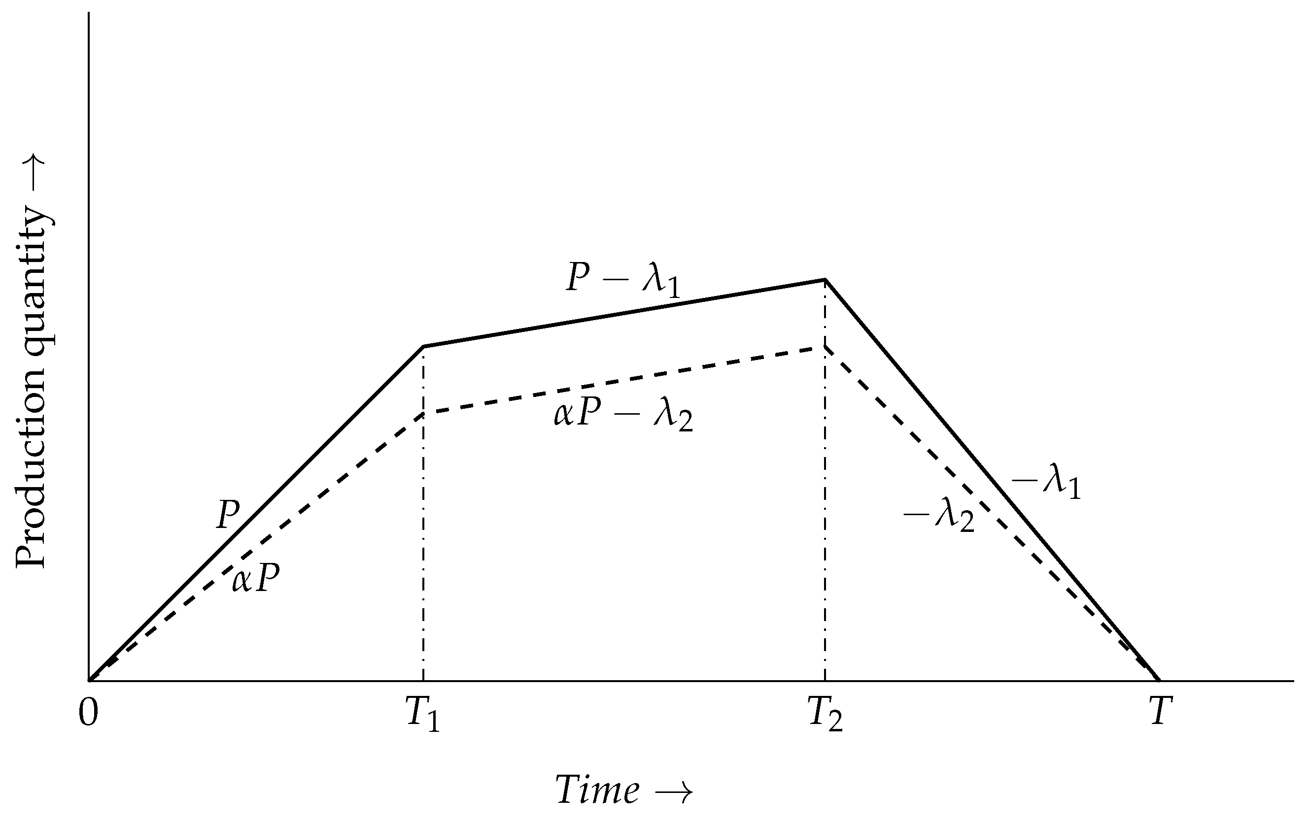
• A production system produces the main product and by-product simultaneously. The production system has two setups: one is for the main product and the other is for the by-product. The demand of the main product (${\lambda }_1$) [2] and by-product (${\lambda }_2$) is constant.
• The production rate of the main product is constant [17]. The by-product is produced simultaneously at a rate of $\alpha P$. As the system transitions to an out-of-control state and produces some defective products [51], rework for the main product and refining process for the by-products take place. The out-of-control rate of the production system $\theta$ has the same effect on both setups.
• Total cycle time is T. $T_1$ is the production time and $T_2$ is the production with reworking time. $T_1$ and $T_2$ are the proportions of T, i.e., $T_1={\delta }_{1}T$ and $T_2={\delta }_{2}T$, where $0<{\delta }_1<1$, $0<{\delta }_2<1$, and ${\delta }_1<{\delta }_2$.
• Machine reliability is a big concern for a production system. If the machine is not reliable, it produces more defective products than the normal rate. An investment is used to improve the reliability of both production and refining processes. An additional investment is used for setup cost reduction for the system [13].
• The production system emits carbon during the entire production time [23]. Carbon emission costs for main products and by-products are different. To be more specific, carbon emission cost due to refining is less to that of production as production is on a large scale, while there are less units to be refined as a by-product is formed at a rate of $\alpha P$, where $\alpha$ is less than one.
• Split-off point is the stage in a production process where the by-products become separately identifiable from the main products. The model and the associated costs are formulated after that split-off point.
• All associated costs related to the main product are higher than that of the by-product. Shortage and lead time are negligible.

4. Formulation of Model

The projected study formulates a production-inventory model without considering Markov chain. The problem description, as stated in Section 3.1, is executed by formulating the total cost of the production-inventory system. Each step of managing the main product and by-product requires some costs such as setup, quality improvement of products, reworking of products, holding of products, machine reliability improvement, and carbon emission costs. These costs are discussed in this section along with the total cost of the production-inventory model. The production system produces the main product at a rate of P and $\alpha P$ is the rate of by-product production. Until $T_1$ is reached, only production is performed. From $T_1$ to $T_2$, both production and demand fulfillment take place. From time $T_2$ to T, only demand is fulfilled and no production occurs (Figure 3).

4.1. Setup Cost

Setup cost refers to the expenses incurred when preparing equipment, machinery, or systems for a specific production task or operation. It is divided into two parts:

•

Setup cost for the main product. The production activity requires a setup and the associated cost is given by S.

•

Setup cost for refining the processing of the by-product. The refining process requires a different setup which constitutes a cost given by $S_1$.

4.2. Production Cost

Production cost is divided into two parts:

•

Production cost of main product. It is given by

$$\begin{array}{cc}& P_c\underset{0}{\overset{T_2}{\int }}Pdt=P_{c}P{T}_2.\end{array}$$

(1)

•

Refining cost of by-product. Refining or processing costs for by-products involve the expenses incurred in separating and processing these secondary products alongside the main product during production. It is given by

$$\begin{array}{cc}& R_c\underset{0}{\overset{T_2}{\int }}\alpha Pdt=R_c\alpha P{T}_2.\end{array}$$

(2)

4.3. Cost of Quality Improvement and Setup Cost Reduction

Quality improvement ($log\theta$) and setup reduction ($logS$) costs are both investments aimed at enhancing operational efficiency and customer satisfaction within a business. G is the annual fractional cost for the investment and $\gamma$ is a positive integer [51]. The investment for these purposes is given by

$$\begin{array}{cc}& G(\gamma -Blog\theta -blogS).\end{array}$$

(3)

4.4. Rework Cost for Main Product

Rework cost refers to the expenses incurred to rectify defects or deficiencies in a product or service that did not meet quality standards during the initial production or delivery process. During production, the machine shifts from an in-control state to out-of-control state; defective units are then produced, which are reworked at a cost given by

$$\begin{array}{cc}& {\displaystyle \frac{C_r\theta {\lambda }_1^{2}T}{2}}.\end{array}$$

(4)

4.5. Reprocessing Cost for By-Product

During the refining process, the machine shifts from an in-control state to out-of-control state, due to which reprocessing is required. The cost associated to this is given by

$$\begin{array}{cc}& {\displaystyle \frac{C_r^1{\theta }_1{\lambda }_2^{2}T}{2}}.\end{array}$$

(5)

4.6. Cost of System Reliability Improvement and Setup Cost Reduction for By-Product

To improve the by-product’s quality improvement (${\theta }_1$) and setup cost reduction ($S_1$), an investment is used. Associated cost is given by

$$\begin{array}{cc}& G^1({\gamma }^1-B^{1}log{\theta }_1-b^{1}log{S}_1).\end{array}$$

(6)

4.7. Holding Cost

Both the main and by-products are stored during [0, T] time. The holding cost is given by

$$\begin{array}{ccc}& & H_c\left[\underset{0}{\overset{T_1}{\int }}Ptdt+\underset{T_1}{\overset{T_2}{\int }}((P-{\lambda }_1)t+{\lambda }_{1}T-P{T}_2)dt+\underset{T_2}{\overset{T}{\int }}{\lambda }_1(T-t)dt\right]+h_c[\underset{0}{\overset{T_1}{\int }}\alpha Ptdt\hfill \\ & & +\underset{T_1}{\overset{T_2}{\int }}((\alpha P-{\lambda }_2)t+{\lambda }_{1}T-\alpha P{T}_2)dt+\underset{T_2}{\overset{T}{\int }}{\lambda }_2(T-t)dt]\hfill \\ & & =H_c\left[{\displaystyle \frac{P{T}_1^2}{2}}+(T_2-T_1)\left({\displaystyle \frac{P-{\lambda }_1}{2}}(T_2+T_1)+{\lambda }_{1}T-P{T}_2\right)+{\displaystyle \frac{{\lambda }_1}{2}}{(T-T_2)}^2\right]\hfill \\ & & +h_c\left[{\displaystyle \frac{\alpha P{T}_1^2}{2}}+(T_2-T_1)\left({\displaystyle \frac{\alpha P-{\lambda }_2}{2}}(T_2+T_1)+{\lambda }_{2}T-\alpha P{T}_2\right)+{\displaystyle \frac{{\lambda }_2{(T-T_2)}^2}{2}}\right].\hfill \end{array}$$

(7)

4.8. Carbon Emissions Cost

Carbon emissions cost is paid for the production system and refining system for main and by-products, respectively. The associated cost is given by

$$\begin{array}{cc}& C_e^1\underset{0}{\overset{T_2}{\int }}Pdt+C_e^2\underset{0}{\overset{T_2}{\int }}\alpha Pdt=C_e^{1}P{T}_2+C_e^2\alpha P{T}_2.\end{array}$$

(8)

4.9. Total Cost

After setting $T_1={\delta }_{1}T$ and $T_2={\delta }_{2}T$ where $0<{\delta }_1<1$, $0<{\delta }_2<1$, and ${\delta }_1<{\delta }_2$, the total cost is given by

$$\begin{array}{ccc}\hfill TC& =& {\displaystyle \frac{1}{T}}[S+S_1+{\displaystyle \frac{C_r\theta {\lambda }_1^{2}T}{2}}+{\displaystyle \frac{C_r^1{\theta }_1{\lambda }_2^{2}T}{2}}+P{\delta }_2(P_c+C_e^1+R_c\alpha +C_e^2\alpha )T+{\displaystyle \frac{P{\delta }_1^2{T}^2}{2}}(H_c+\alpha h_c)\hfill \\ & +& T^2{\displaystyle \frac{{(1-{\delta }_2)}^2}{2}}({\lambda }_1{H}_c+{\lambda }_2{h}_c)+{\displaystyle \frac{({\delta }_2^2-{\delta }_1^2)T^2}{2}}(H_c(P-{\lambda }_1)+h_c(\alpha P-{\lambda }_2))\hfill \\ & +& ({\delta }_2-{\delta }_1)T^2(H_c{\lambda }_1+h_c{\lambda }_2)+({\delta }_2-{\delta }_1){\delta }_2{T}^{2}P(H_c-\alpha h_c)]+G(\gamma -Blog\theta -blogS)\hfill \\ & +& G^1({\gamma }^1-B^{1}log{\theta }_1-b^{1}log{S}_1).\hfill \end{array}$$

(9)

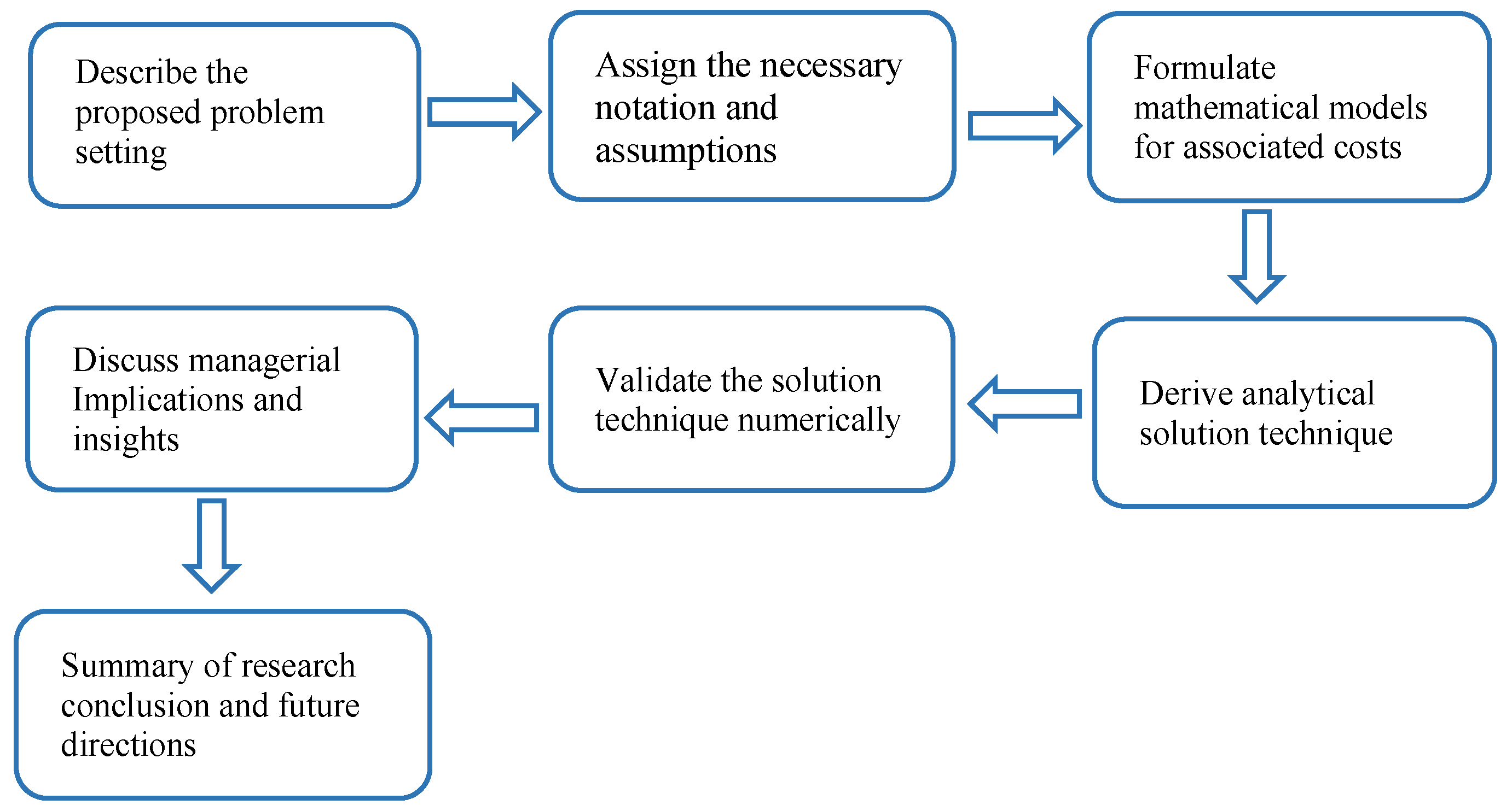
5. Solution Methodology

Equation (9) is solved for the global minimum cost using classical optimization. The necessary and sufficient conditions are described below for Equation (9).

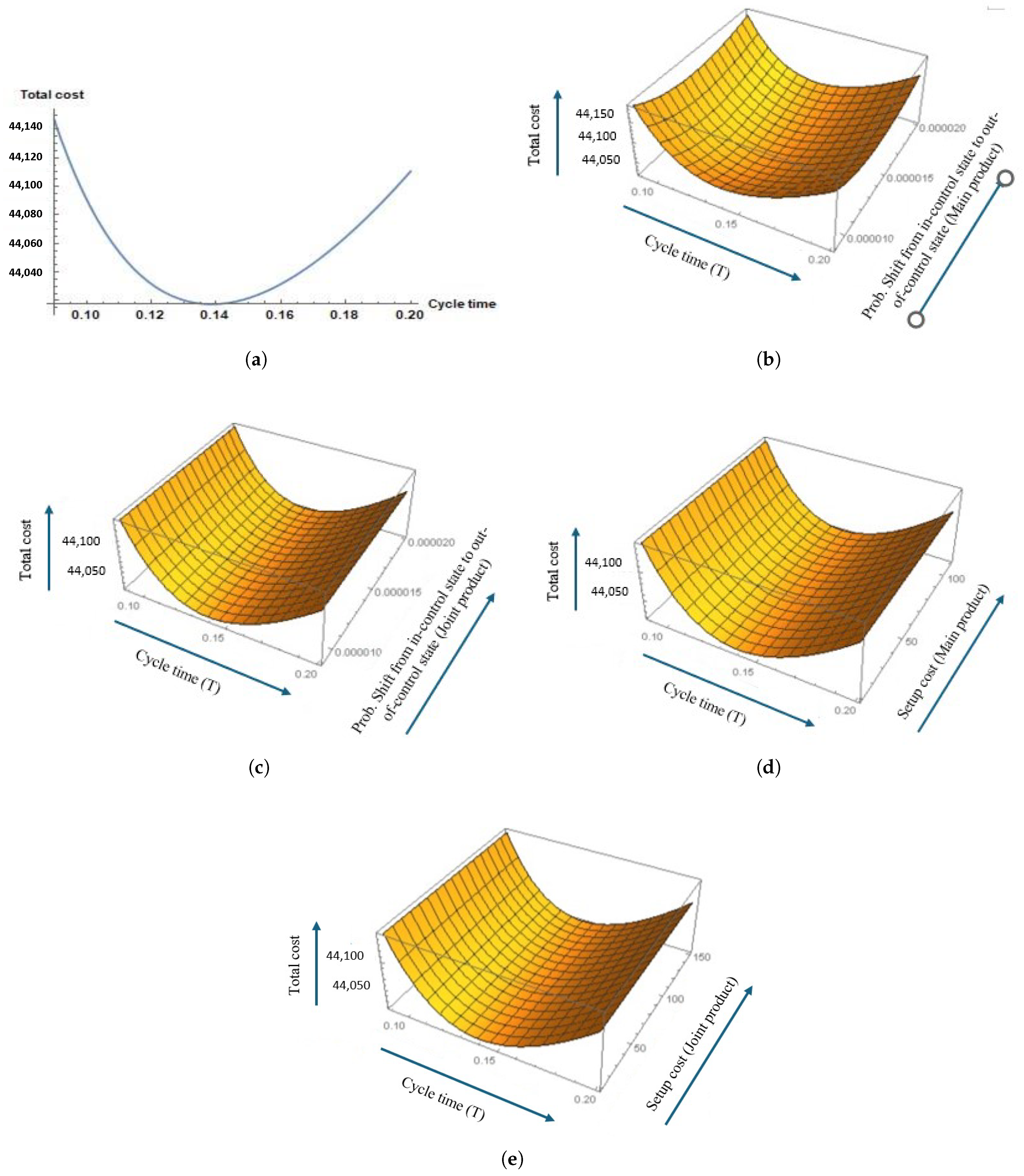
5.1. Necessary Condition of Classical Optimization for Optimality

Differentiating Equation (9) partially with respect to the decision variables $T,S,S_1,\theta ,$ and ${\theta }_1$ and equating to zero, one can obtain the values of decision variables. These can be represented as

$$\begin{array}{ccc}\hfill {\displaystyle \frac{\partial TC}{\partial T}}& =& -{\displaystyle \frac{S+S_1}{T^2}}+(P{\delta }_1^2(H_c+\alpha h_c)+{(1-{\delta }_2)}^2({\lambda }_1{H}_c+{\lambda }_2{h}_c)+({\delta }_2^2-{\delta }_1^2)(H_c(P-{\lambda }_1)\hfill \\ & & +h_c(\alpha P-{\lambda }_2))+2({\delta }_2-{\delta }_1)(H_c{\lambda }_1+h_c{\lambda }_2)+2({\delta }_2-{\delta }_1){\delta }_{2}P(H_c-\alpha h_c))/2=0\hfill \\ & & \mathrm{implies}\hfill \\ \hfill T^{\ast }& =& \sqrt{[}\left(2(S+S_1)\right)/(P{\delta }_1^2(H_c+\alpha h_c)+{(1-{\delta }_2)}^2({\lambda }_1{H}_c+{\lambda }_2{h}_c)+({\delta }_2^2-{\delta }_1^2)(H_c\hfill \\ & & (P-{\lambda }_1)+h_c(\alpha P-{\lambda }_2))+2({\delta }_2-{\delta }_1)(H_c{\lambda }_1+h_c{\lambda }_2)+2({\delta }_2-{\delta }_1){\delta }_{2}P(H_c-\alpha h_c))]\hfill \\ \hfill {\displaystyle \frac{\partial TC}{\partial \theta }}& =& {\displaystyle \frac{C_{r}T{\lambda }_1^2}{T}}-{\displaystyle \frac{GB}{\theta }}=0\mathrm{implies}{\theta }^{\ast }={\displaystyle \frac{2GB}{C_r{\lambda }_1^2}}\hfill \\ \hfill {\displaystyle \frac{\partial TC}{\partial {\theta }_1}}& =& {\displaystyle \frac{C_r^{1}T{\lambda }_2^2}{T}}-{\displaystyle \frac{G^1{B}^1}{{\theta }_1}}=0\mathrm{implies}{\theta }_1^{\ast }={\displaystyle \frac{2G^1{B}^1}{C_r^1{\lambda }_2^2}}\hfill \\ \hfill {\displaystyle \frac{\partial TC}{\partial S}}& =& {\displaystyle \frac{1}{T}}-{\displaystyle \frac{Gb}{S}}=0\mathrm{implies}{S}^{\ast }=GbT\hfill \\ \hfill {\displaystyle \frac{\partial TC}{\partial S_1}}& =& {\displaystyle \frac{1}{T}}-{\displaystyle \frac{G^1{b}^1}{S_1}}=0\mathrm{implies}{S}_1^{\ast }=G^1{b}^{1}T.\hfill \end{array}$$

(10)

5.2. Sufficient Conditions of Classical Optimization for Optimality

To obtain sufficient conditions, it is required to calculate the values of the principal minors of the Hessian matrix.

Theorem 1.

The values of all principal minors of 4 × 4 Hessian matrix are positive in sign at optimal values of decision variables in Equation (10). Therefore, the total cost function is positive definite, which indicates its global minimality with respect to decision variables.

Proof. 

The Hessian matrix is given by

$$\begin{array}{cc}& H_{55}=\left(\begin{array}{ccccc}{\displaystyle \frac{{\partial }^{2}TC}{\partial T^2}}& {\displaystyle \frac{{\partial }^{2}TC}{\partial T\partial \theta }}& {\displaystyle \frac{{\partial }^{2}TC}{\partial T\partial {\theta }_1}}& {\displaystyle \frac{{\partial }^{2}TC}{\partial T\partial S}}& {\displaystyle \frac{{\partial }^{2}TC}{\partial T\partial S_1}}\\ {\displaystyle \frac{{\partial }^{2}TC}{\partial \theta \partial T}}& {\displaystyle \frac{{\partial }^{2}TC}{\partial {\theta }^2}}& {\displaystyle \frac{{\partial }^{2}TC}{\partial \theta \partial {\theta }_1}}& {\displaystyle \frac{{\partial }^{2}TC}{\partial \theta \partial S}}& {\displaystyle \frac{{\partial }^{2}TC}{\partial \theta \partial S_1}}\\ {\displaystyle \frac{{\partial }^{2}TC}{\partial {\theta }_1\partial T}}& {\displaystyle \frac{{\partial }^{2}TC}{\partial {\theta }_1\partial \theta }}& {\displaystyle \frac{{\partial }^{2}TC}{\partial {\theta }_1^2}}& {\displaystyle \frac{{\partial }^{2}TC}{\partial {\theta }_1\partial S}}& {\displaystyle \frac{{\partial }^{2}TC}{\partial {\theta }_1\partial S_1}}\\ {\displaystyle \frac{{\partial }^{2}TC}{\partial S\partial T}}& {\displaystyle \frac{{\partial }^{2}TC}{\partial S\partial \theta }}& {\displaystyle \frac{{\partial }^{2}TC}{\partial S\partial {\theta }_1}}& {\displaystyle \frac{{\partial }^{2}TC}{\partial S^2}}& {\displaystyle \frac{{\partial }^{2}TC}{\partial S\partial S_1}}\\ {\displaystyle \frac{{\partial }^{2}TC}{\partial S_1\partial T}}& {\displaystyle \frac{{\partial }^{2}TC}{\partial S_1\partial \theta }}& {\displaystyle \frac{{\partial }^{2}TC}{\partial S_1\partial {\theta }_1}}& {\displaystyle \frac{{\partial }^{2}TC}{\partial S_1\partial S}}& {\displaystyle \frac{{\partial }^{2}TC}{\partial S_1^2}}\end{array}\right)\hfill \end{array}$$

Second-order partial derivatives of decision variables are ${\displaystyle \frac{{\partial }^{2}TC}{\partial T^2}}={\displaystyle \frac{2(S+S_1)}{T^3}},{\displaystyle \frac{{\partial }^{2}TC}{\partial {\theta }^2}}={\displaystyle \frac{GB}{{\theta }^2}},{\displaystyle \frac{{\partial }^{2}TC}{\partial {\theta }_1^2}}={\displaystyle \frac{G^1{B}^1}{{\theta }_1^2}},{\displaystyle \frac{{\partial }^{2}TC}{\partial S^2}}={\displaystyle \frac{Gb}{S^2}},{\displaystyle \frac{{\partial }^{2}TC}{\partial S_1^2}}={\displaystyle \frac{G^1{b}^1}{S_1^2}}$.

Mixed partial derivatives of decision variables are zero, i.e., ${\displaystyle \frac{{\partial }^{2}TC}{\partial \theta \partial T}}={\displaystyle \frac{{\partial }^{2}TC}{\partial S\partial \theta }}={\displaystyle \frac{{\partial }^{2}TC}{\partial \theta \partial {\theta }_1}}={\displaystyle \frac{{\partial }^{2}TC}{\partial {\theta }_1\partial S}}={\displaystyle \frac{{\partial }^{2}TC}{\partial S\partial S_1}}={\displaystyle \frac{{\partial }^{2}TC}{\partial \theta \partial S_1}}={\displaystyle \frac{{\partial }^{2}TC}{\partial {\theta }_1\partial T}}={\displaystyle \frac{{\partial }^{2}TC}{\partial S\partial T}}={\displaystyle \frac{{\partial }^{2}TC}{\partial S_1\partial T}}={\displaystyle \frac{{\partial }^{2}TC}{\partial S_1\partial {\theta }_1}}=0$.

First-order 1 × 1 principal minor is ${\displaystyle \frac{{\partial }^{2}TC}{\partial T^2}}={\displaystyle \frac{2(S+S_1)}{T^3}}$, which is positive as all parameters are positive.

The second-order 2 × 2 principal minor is

$$\begin{array}{cc}& \left|\begin{array}{cc}{\displaystyle \frac{{\partial }^{2}TC}{\partial T^2}}& {\displaystyle \frac{{\partial }^{2}TC}{\partial T\partial \theta }}\\ {\displaystyle \frac{{\partial }^{2}TC}{\partial \theta \partial T}}& {\displaystyle \frac{{\partial }^{2}TC}{\partial {\theta }^2}}\end{array}\right|={\displaystyle \frac{{\partial }^{2}TC}{\partial {\theta }^2}}{\displaystyle \frac{{\partial }^{2}TC}{\partial T^2}}={\displaystyle \frac{GB}{{\theta }^2}}{\displaystyle \frac{2(S+S_1)}{T^3}}\hfill \end{array}$$

which is positive as all parameters are positive.

The third-order 3 × 3 principal minor is

$$\begin{array}{cc}& \left|\begin{array}{ccc}{\displaystyle \frac{{\partial }^{2}TC}{\partial T^2}}& {\displaystyle \frac{{\partial }^{2}TC}{\partial T\partial \theta }}& {\displaystyle \frac{{\partial }^{2}TC}{\partial T\partial {\theta }_1}}\\ {\displaystyle \frac{{\partial }^{2}TC}{\partial \theta \partial T}}& {\displaystyle \frac{{\partial }^{2}TC}{\partial {\theta }^2}}& {\displaystyle \frac{{\partial }^{2}TC}{\partial \theta \partial {\theta }_1}}\\ {\displaystyle \frac{{\partial }^{2}TC}{\partial {\theta }_1\partial T}}& {\displaystyle \frac{{\partial }^{2}TC}{\partial {\theta }_1\partial \theta }}& {\displaystyle \frac{{\partial }^{2}TC}{\partial {\theta }_1^2}}\end{array}\right|={\displaystyle \frac{{\partial }^{2}TC}{\partial {\theta }_1^2}}{\displaystyle \frac{{\partial }^{2}TC}{\partial {\theta }^2}}{\displaystyle \frac{{\partial }^{2}TC}{\partial T^2}}={\displaystyle \frac{G^1{B}^1}{{\theta }_1^2}}{\displaystyle \frac{GB}{{\theta }^2}}{\displaystyle \frac{2(S+S_1)}{T^3}}\hfill \end{array}$$

which is positive as all parameters are positive.

The fourth-order 4 × 4 principal minor is

$$\begin{array}{cc}& \left|\begin{array}{cccc}{\displaystyle \frac{{\partial }^{2}TC}{\partial T^2}}& {\displaystyle \frac{{\partial }^{2}TC}{\partial T\partial \theta }}& {\displaystyle \frac{{\partial }^{2}TC}{\partial T\partial {\theta }_1}}& {\displaystyle \frac{{\partial }^{2}TC}{\partial T\partial S}}\\ {\displaystyle \frac{{\partial }^{2}TC}{\partial \theta \partial T}}& {\displaystyle \frac{{\partial }^{2}TC}{\partial {\theta }^2}}& {\displaystyle \frac{{\partial }^{2}TC}{\partial \theta \partial {\theta }_1}}& {\displaystyle \frac{{\partial }^{2}TC}{\partial \theta \partial S}}\\ {\displaystyle \frac{{\partial }^{2}TC}{\partial {\theta }_1\partial T}}& {\displaystyle \frac{{\partial }^{2}TC}{\partial {\theta }_1\partial \theta }}& {\displaystyle \frac{{\partial }^{2}TC}{\partial {\theta }_1^2}}& {\displaystyle \frac{{\partial }^{2}TC}{\partial {\theta }_1\partial S}}\\ {\displaystyle \frac{{\partial }^{2}TC}{\partial S\partial T}}& {\displaystyle \frac{{\partial }^{2}TC}{\partial S\partial \theta }}& {\displaystyle \frac{{\partial }^{2}TC}{\partial S\partial {\theta }_1}}& {\displaystyle \frac{{\partial }^{2}TC}{\partial S^2}}\end{array}\right|={\displaystyle \frac{{\partial }^{2}TC}{\partial S^2}}{\displaystyle \frac{{\partial }^{2}TC}{\partial {\theta }_1^2}}{\displaystyle \frac{{\partial }^{2}TC}{\partial {\theta }^2}}{\displaystyle \frac{{\partial }^{2}TC}{\partial T^2}}={\displaystyle \frac{Gb}{S^2}}{\displaystyle \frac{G^1{B}^1}{{\theta }_1^2}}{\displaystyle \frac{GB}{{\theta }^2}}{\displaystyle \frac{2(S+S_1)}{T^3}}\hfill \end{array}$$

which is positive as all parameters are positive.

The fifth-order 5 × 5 principal minor is

$$\begin{array}{cc}& \left|\begin{array}{ccccc}{\displaystyle \frac{{\partial }^{2}TC}{\partial T^2}}& {\displaystyle \frac{{\partial }^{2}TC}{\partial T\partial \theta }}& {\displaystyle \frac{{\partial }^{2}TC}{\partial T\partial {\theta }_1}}& {\displaystyle \frac{{\partial }^{2}TC}{\partial T\partial S}}& {\displaystyle \frac{{\partial }^{2}TC}{\partial T\partial S_1}}\\ {\displaystyle \frac{{\partial }^{2}TC}{\partial \theta \partial T}}& {\displaystyle \frac{{\partial }^{2}TC}{\partial {\theta }^2}}& {\displaystyle \frac{{\partial }^{2}TC}{\partial \theta \partial {\theta }_1}}& {\displaystyle \frac{{\partial }^{2}TC}{\partial \theta \partial S}}& {\displaystyle \frac{{\partial }^{2}TC}{\partial \theta \partial S_1}}\\ {\displaystyle \frac{{\partial }^{2}TC}{\partial {\theta }_1\partial T}}& {\displaystyle \frac{{\partial }^{2}TC}{\partial {\theta }_1\partial \theta }}& {\displaystyle \frac{{\partial }^{2}TC}{\partial {\theta }_1^2}}& {\displaystyle \frac{{\partial }^{2}TC}{\partial {\theta }_1\partial S}}& {\displaystyle \frac{{\partial }^{2}TC}{\partial {\theta }_1\partial S_1}}\\ {\displaystyle \frac{{\partial }^{2}TC}{\partial S\partial T}}& {\displaystyle \frac{{\partial }^{2}TC}{\partial S\partial \theta }}& {\displaystyle \frac{{\partial }^{2}TC}{\partial S\partial {\theta }_1}}& {\displaystyle \frac{{\partial }^{2}TC}{\partial S^2}}& {\displaystyle \frac{{\partial }^{2}TC}{\partial S\partial S_1}}\\ {\displaystyle \frac{{\partial }^{2}TC}{\partial S_1\partial T}}& {\displaystyle \frac{{\partial }^{2}TC}{\partial S_1\partial \theta }}& {\displaystyle \frac{{\partial }^{2}TC}{\partial S_1\partial {\theta }_1}}& {\displaystyle \frac{{\partial }^{2}TC}{\partial S_1\partial S}}& {\displaystyle \frac{{\partial }^{2}TC}{\partial S_1^2}}\end{array}\right|={\displaystyle \frac{{\partial }^{2}TC}{\partial S_1^2}}{\displaystyle \frac{{\partial }^{2}TC}{\partial S^2}}{\displaystyle \frac{{\partial }^{2}TC}{\partial {\theta }_1^2}}{\displaystyle \frac{{\partial }^{2}TC}{\partial {\theta }^2}}{\displaystyle \frac{{\partial }^{2}TC}{\partial T^2}}={\displaystyle \frac{G^1{b}^1}{S_1^2}}{\displaystyle \frac{Gb}{S^2}}{\displaystyle \frac{G^1{B}^1}{{\theta }_1^2}}{\displaystyle \frac{GB}{{\theta }^2}}{\displaystyle \frac{2(S+S_1)}{T^3}},\hfill \end{array}$$

which is positive as all parameters are positive. All other second-order derivatives are zero. Thus, the total cost in Equation (10) is a convex function with a global minimum. □

5.3. Robustness of the Solution to Parameter Uncertainty

A comparison with the total cost to parameter uncertainty is tested in this section. Two cases are tested: the main product’s demand uncertainty and cost uncertainty. One cost is tested for the cost uncertainty parameter and it will be similar for the other cost parameters.

5.3.1. Robustness of the Solution to Uncertain Demand Parameter

The market demand of the main product contains some uncertainty. The uncertain market demand of the main product is represented as ${\tilde{\lambda }}_1$. If ${\tilde{\lambda }}_1$ follows a triangular fuzzy number defined within a range of (${\epsilon }_1,{\epsilon }_2$), then the uncertain market demand of the main product can be represented as ${\tilde{\lambda }}_1=({\lambda }_1-{\epsilon }_1,{\lambda }_1,{\lambda }_1+{\epsilon }_2)$. The membership function of the triangular fuzzy number is ${\mu }_{{\tilde{\lambda }}_1}\left(\alpha \right)=\left\{\begin{array}{cc}{\displaystyle \frac{\alpha -({\lambda }_1-{\epsilon }_1)}{{\epsilon }_1}},\hfill & {\lambda }_1-{\epsilon }_1\le \alpha \le {\lambda }_1;\hfill \\ {\displaystyle \frac{{\lambda }_1+{\epsilon }_2-\alpha }{{\epsilon }_2}},\hfill & {\lambda }_1\le \alpha \le {\lambda }_1+{\epsilon }_2;\hfill \\ 0,\hfill & \mathrm{otherwise}.\hfill \end{array}\right.$

The centroid of the membership function ${\mu }_{{\tilde{\lambda }}_1}\left(\alpha \right)$ is [52]

$$\begin{array}{c}\hfill {\lambda }_1^{\prime }={\lambda }_1+{\displaystyle \frac{{\epsilon }_2-{\epsilon }_1}{3}}.\end{array}$$

(11)

After defuzzification using the centroid, the fuzzy total cost of the production system is

$$\begin{array}{ccc}\hfill \widetilde{TC}(T,\theta ,{\theta }_1,S,S_1)=& & TC+{\displaystyle \frac{H_c({\epsilon }_2-{\epsilon }_1)T}{6}}\left[{(1-{\delta }_2)}^2+({\delta }_2^2-{\delta }_1^2)+({\delta }_2-{\delta }_1)\right]\hfill \\ & & +{\displaystyle \frac{C_r\theta }{6}}\left[{\epsilon }_1^2+{\epsilon }_2^2+2{\lambda }_1({\epsilon }_2-{\epsilon }_1)\right].\hfill \end{array}$$

(12)

The first term of the above uncertain cost (Equation (12)) is the same as in Equation (9) without uncertainty. The second and third terms of the above uncertain cost of the production system appear because of the uncertain nature of the demand of the main product. That is, there is some information about the demand that is not certain and these additional costs are required to process this uncertain information. This proves that the total uncertain cost is always greater than the cost without uncertainty. Thus, the obtained cost in Equation (10) is the minimum. The consideration of a demand parameter uncertainty increases the total cost of the system. However, this concluding remark is already established in literature [52]. Thus,

$$\begin{array}{c}\hfill TC(T,\theta ,{\theta }_1,S,S_1)<\widetilde{TC}(T,\theta ,{\theta }_1,S,S_1).\end{array}$$

(13)

5.3.2. Robustness of the Solution to Uncertain Cost Parameter

The cost of the production system is considered as uncertain. The uncertain part of the cost ($\alpha$) follows a triangular fuzzy number. The production cost of the main product is taken as a uncertain cost. With three points of a triangle $X=(\alpha -{\epsilon }_1,\alpha ,\alpha +{\epsilon }_2)$, the membership function ${\mu }_{\tilde{X}}\left(\alpha \right)=\left\{\begin{array}{cc}{\displaystyle \frac{\alpha -(X-{\epsilon }_1)}{{\epsilon }_1}},\hfill & X-{\epsilon }_1\le \alpha \le X;\hfill \\ {\displaystyle \frac{X+{\epsilon }_2-\alpha }{{\epsilon }_2}},\hfill & X\le \alpha \le X+{\epsilon }_2;\hfill \\ 0,\hfill & \mathrm{otherwise}.\hfill \end{array}\right.$

The distance between the fuzzy number $\tilde{\alpha }$ to the point of the fuzzy set ${\tilde{Y}}_{{\mu }_{\tilde{X}}\left(\alpha \right)}$ using the signed distance method is [28]

$$\begin{array}{c}\hfill d(\tilde{\alpha },\tilde{Y})=\alpha +{\displaystyle \frac{{\epsilon }_2-{\epsilon }_1}{4}}.\end{array}$$

(14)

Using the signed distance method to defuzzify the fuzzy production cost of the main product, the cost is written as

$$\begin{array}{c}\hfill \left[P_c+{\displaystyle \frac{{\epsilon }_2-{\epsilon }_1}{4}}\right]P{\delta }_2.\end{array}$$

(15)

Other costs can be similarly expressed with uncertainty. The total fuzzy cost of the production system can be written as

$$\begin{array}{c}\hfill \widetilde{T{C}_1}(T,\theta ,{\theta }_1,S,S_1)=TC+{\displaystyle \frac{{\epsilon }_2-{\epsilon }_1}{4}}P{\delta }_2.\end{array}$$

(16)

The first part of the above fuzzy Equation (16) is the same as Equation (9). The second part of the fuzzy total cost appears because of the information uncertainty. It increases the total cost of the system. Thus, the total cost of the model in Equation (10) is the minimum than the uncertain total cost in Equation (16). This phenomenon has already been established in the literature [28]. Thus,

$$\begin{array}{c}\hfill TC(T,\theta ,{\theta }_1,S,S_1)<\widetilde{T{C}_1}(T,\theta ,{\theta }_1,S,S_1).\end{array}$$

(17)

Thus, it is established theoretically from Equations (13) and (17) that the total cost of the proposed model is global minimum than any uncertainty in the parameters, either in demand or in cost. The uncertainty discussions show that the total cost undoubtedly increases compared with the obtained cost. Thus, the obtained result is robust.

6. Numerical Example

Input data for the numerical testing of the model are given in

Table 2. Input values of parameters.

Parameters	Values	Parameters	Values	Parameters	Values
$G\left(USD\right)$	0.99	$P_c$ (USD/unit)	5	${\delta }_1$	0.3
${\delta }_2$	0.7	$\gamma$	0.5	b	458
$h_c$ (USD/unit)	0.3	$H_c$ (USD/unit)	0.5	$C_e^1$ (USD/unit)	0.2
B	450	$R_c$ (USD/unit)	1.3	$\alpha$	0.1
P (unit/year)	10,000	$B^1$	150	$b^1$	50
${\lambda }_1$ (unit/year)	8000	$G^1\left(USD\right)$	1.5	${\gamma }^1$	0.5
$C_r$ (USD/unit)	1	$C_r^1$ (USD/unit)	0.6	${\lambda }_2$ (unit/year)	4000
$C_e^2$ (USD/unit)	0.1

. The model can be related to several industries such as the soap industry with glycerine as a by-product, or the sugar industry with molasses as the by-product. However, $\alpha$ can vary accordingly and rework can be replaced by rework. Optimal solutions are given in

Table 3. Optimal values of decision variables and total cost.

Decision Variables	Optimum Values	Decision Variables	Optimum Values
T	0.1386 year	$\theta$	0.000014
${\theta }_1$	0.000047	S	USD 63.47/setup
$S_1$	USD 31.18/setup

. Total cost $TC$ of the sustainable production system is USD 44,017.5/year. Figure 4a–e showcase the concavity between different decision variables. Results show that the quality improvement of by-products is more important than the quality improvement of the main product. The relevant data were taken from [42,51]. The by-product data were taken from [53] for the soap industry. The data have been modified based on the convergence of the algorithm.

7. Sensitivity Analysis

Table 4. Sensitivity analysis of key parameters.

Parameters	Variation	T	$\mathit{\theta }$	${\mathit{\theta }}_1$	S	${\mathit{S}}_1$	$\mathit{TC}$ (Changes in %)
	$+50\%$	+0.096			+43.87	+21.55	+0.006
$H_c$	$+25\%$	+0.11			+51.88	+25.49	+0.003
	$-25\%$	+0.18	−	−	+81.73	+40.15	−0.004
	$-50\%$	+0.25			+114.75	+56.37	−0.007
	$+50\%$	+0.132			+60.27	+29.61	+0.0008
$h_c$	$+25\%$	+0.135			+61.83	+30.37	+0.0004
	$-25\%$	+0.142	−	−	+65.2	+32.03	−0.0004
	$-50\%$	+0.146			+67.03	+32.93	−0.0007
	$+50\%$	+0.185	+0.00002		+127.13	+41.64	+0.033
G	$+25\%$	+0.162	+0.000017		+92.64	+36.41	+0.017
	$-25\%$	+0.115	+0.00001	−	+39.62	+25.95	−0.019
	$-50\%$	+0.092	+0.000007		+21.09	+20.73	−l0.04
	$+50\%$						+0.4
$P_c$	$+25\%$						+0.2
	$-25\%$	−	−	−	−	−	−0.2
	$-50\%$						−0.4
	$+50\%$		+0.0000211				+0.06
B	$+25\%$		+0.000017				+0.04
	$-25\%$	−	+0.000011	−	−	−	−0.03
	$-50\%$		+0.000007				−0.06
	$+50\%$		+0.00001				+0.004
$C_r$	$+25\%$		+0.000011				+0.002
	$-25\%$	−	+0.000019	−	−	−	−0.003
	$-50\%$		+0.00002				−0.004
	$+50\%$			+0.00002			+0.003
$C_r^1$	$+25\%$			+0.00003			+0.0015
	$-25\%$	−	−	+0.00004	−	−	−0.0017
	$-50\%$			+0.00009			−0.003
	$+50\%$						+0.01
$R_c$	$+25\%$						+0.005
	$-25\%$	−	−	−	−	−	−0.005
	$-50\%$						−0.01
	$+50\%$						+0.016
$C_e^1$	$+25\%$						+0.008
	$-25\%$	−	−	−	−	−	−0.008
	$-50\%$						−0.016
	$+50\%$						+0.0008
$C_e^2$	$+25\%$						+0.0004
	$-25\%$	−	−	−	−	−	−0.0004
	$-50\%$						−0.0008
	$+50\%$	0.161			+73.92	+54.48	−0.01
$b^1$	$+25\%$	+0.15			+68.7	+42.19	−0.005
	$-25\%$	+0.13	−	−	+58.24	+21.46	+0.004
	$-50\%$	+0.112			+53.02	+13.02	+0.01
	$+50\%$	+0.181			+93.92	+59.48	−0.01
${\lambda }_1$	$+25\%$	+0.16			+78.7	+48.19	−0.005
	$-25\%$	+0.13	−	−	+58.24	+29.46	+0.004
	$-50\%$	+0.112			+43.02	+19.02	+0.01

− No change.

gives the sensitivity analysis.

Table 5. Time proportion ${\delta }_1$ behavior for production time $T_1$.

${\mathit{\delta }}_1$	T	$\mathit{\theta }$	${\mathit{\theta }}_1$	S	${\mathit{S}}_1$	$\mathit{TC}$ (Changes in %)
0.1	0.0942	−	−	43.144	21.195	−0.004
0.2	0.113	−	−	51.812	25.45	−0.007
0.3	0.138582	−	−	63.47	31.18	0
0.4	0.174	−	−	79.73	39.17	−0.01
0.5	0.226	−	−	103.5	50.84	−0.18
0.6	0.307	−	−	140.6	69.05	−0.023
0.7	0.446	−	−	204.12	100.28	−0.028
0.8	0.724	−	−e	331.55	162.88	−0.036

− No change.

and

Table 6. Time proportion ${\delta }_2$ behavior for production and demand time $T_2$.

${\mathit{\delta }}_2$	T	$\mathit{\theta }$	${\mathit{\theta }}_1$	S	${\mathit{S}}_1$	$\mathit{TC}$ (Changes in %)
0.2	0.7623	−	−	349.123	171.512	−0.64
0.3	0.4516	−	−	206.82	101.603	−0.51
0.4	0.307	−	−	140.65	69.099	−0.38
0.5	0.225	−	−	103.22	50.71	−0.26
0.6	0.174	−	−	79.56	39.08	−0.13
0.7	0.13852	−	−	63.4709	31.1809	0
0.8	0.11346	−	−	51.96	25.53	+0.11
0.9	0.0948	−	−	43.41	21.32	+0.24
1	0.0805	−	−	36.85	18.11	+0.36

− No change.

show the behavior of ${\delta }_1$ and ${\delta }_2$ on total cost and decision variables.

Figure 5 shows a graphical representation of the sensitivity analysis.

•

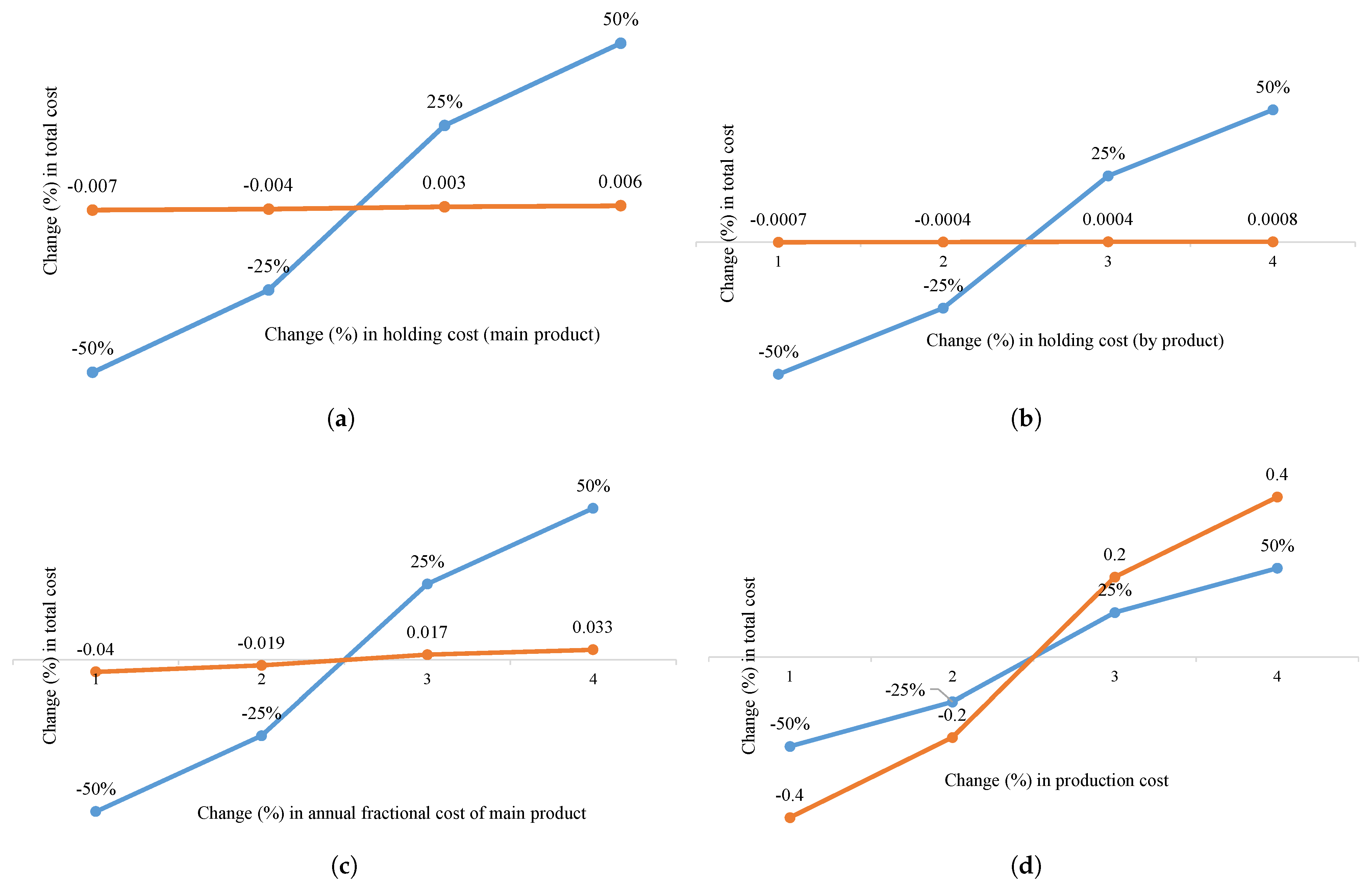
The production cost is the most crucial. By increasing production cost to +50%, total cost increases to 0.4%. Decision makers should make some strategy to lower this. Production costs can be lowered through various means, including improving efficiency in processes, optimizing resource utilization, implementing automation where feasible, negotiating better prices with suppliers, and investing in technology to reduce waste and downtime. Increasing manufacturing volume and spreading fixed costs over a higher output are ways to take advantage of economies of scale. Over time, expenses can be further reduced by identifying and eliminating production process inefficiencies through continuous improvement efforts like Six Sigma and lean manufacturing.

•

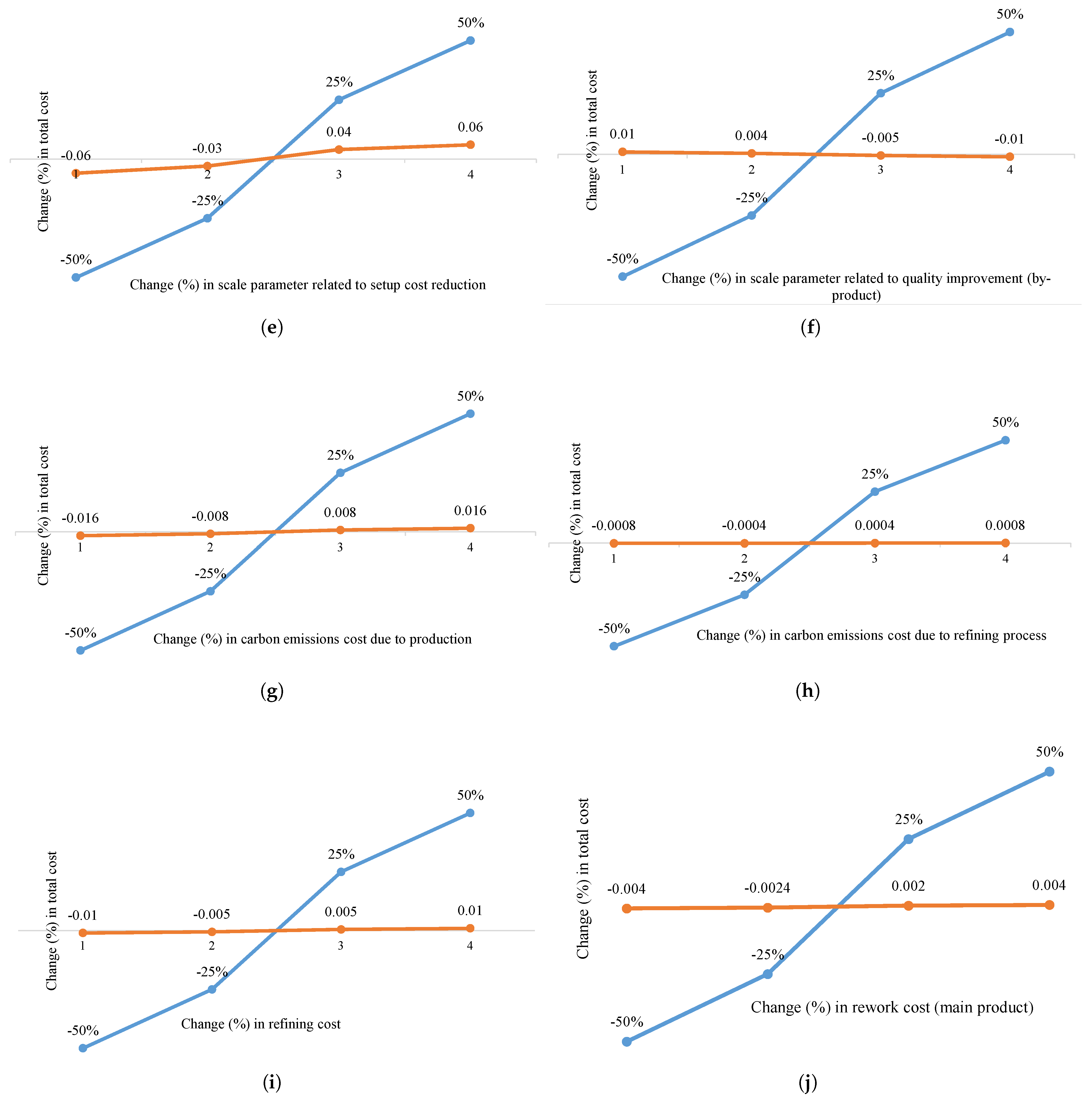
The scaling parameter for the setup cost reduction function is quite sensitive. By increasing the parameter value to +50%, the total cost increases to 0.06%. Refining cost has a significant impact on total cost. By increasing refining/processing cost to +50%, total cost increases to 0.01%. Production cost, carbon emission cost due to production, and refining cost do not affect decision variables.

•

An increase in annual fraction cost of capital investment, i.e., G, increases T, $\theta$, ${\theta }_1$, S, and $S_1$. An increase in G to +50% increases the system’s total cost to 0.033%. The holding cost of the main product is more crucial than the by-product’s. By increasing the holding cost of the main product to +50%, the system’s total cost increases by 0.006%, while the holding cost of the by-product increases to 0.0008%.

•

By increasing the holding cost of both main and by-products, cycle time decreases, i.e., T. This can be governed by the fact that when holding costs increase, it creates a financial incentive for businesses to minimize the time they hold onto an inventory. This prompts them to streamline their operations, reduce excess inventory, and accelerate turnover. Because it becomes more expensive to hold onto inventory for extended periods, this reduces the time it takes for inventory to move through the supply chain. In essence, higher holding costs push businesses to adopt more efficient inventory management practices, ultimately reducing time spent in inventory storage.

•

An increment in scale parameter related to product quality improvement for the by-product, i.e., $b^1$, increases cycle time, setup cost for production, and refining. An increase in $b^1$ to 50% decreases the system’s cost to 0.01%.

•

As ${\delta }_1$ increases, S and $S_1$ increase, but the total cost decreases. Setup costs increase when production time increases primarily because longer production times necessitate more frequent setups. The longer production times can lead to increased downtime between production runs, resulting in more frequent equipment adjustments and maintenance, further driving up setup costs. Therefore, as production time increases, setup costs rise due to the need for additional setup activities and associated expenses.

•

Total cost decreases when the production time increases due to the principle of economies of scale. As production time lengthens, the fixed costs associated with production, such as overhead expenses and equipment depreciation, are spread over larger units produced. This spreading effect reduces the fixed cost per unit, leading to lower average costs. As ${\delta }_2$ increases, S and $S_1$ decrease, but the total cost increases.

8. Implications

• Industries dealing with by-products face unique challenges and opportunities due to the nature of their production processes. Multiple distinct outputs are derived from a single manufacturing process [54]. These by-products share common resources, production inputs, production processes, and market positioning [55].
• Maintaining by-products helps support a circular economy by reducing waste and maximizing resource efficiency. Instead of discarding by-products as waste, they can be reused, repurposed, or transformed into new materials or products, thus extending their life cycle. This not only conserves raw materials and energy but also minimizes environmental impact, supports innovation, and creates economic value from what would otherwise be discarded.
• Carbon emissions are directly related to climate change [56]. Every industry has taken serious measures for emissions from the industry under government supervision. Uniting small, medium, and large industries under one umbrella for climate change is the key to successfully establishing sustainability [20,57]. Controlling carbon emissions from industries can fulfill the environmental goal of sustainability.
• The management of by-products is a sustainable practice for industries whose main products produce one or more by-products. Without the proper management of by-products, the generation of pollution and waste would increase. These by-products serve as inputs for other industries, such as construction, automotive, and plastic manufacturing, contributing to the overall value chain [56]. This creates new industries and jobs (social), reduces waste (environmental), and generates revenue (economic). Thus, by-product management fulfills three pillars of sustainability.
• One of the primary implications of industries with by-products is the need for efficient resource utilization and production planning. Since multiple products are produced simultaneously, companies must carefully allocate resources such as raw materials and equipment to optimize production efficiency and minimize waste [54,58]. This requires sophisticated production planning and scheduling systems to minimize cost [59,60].
• Industries dealing with by-products are diverse and span various sectors, showcasing the versatility and potential of maximizing resource utilization [61,62]. In the agricultural sector, livestock farming is a prominent example of multiple products derived from the same production process [63,64]. For instance, in the dairy industry, milk is the primary product, but the process also yields by-products such as whey, which is rich in proteins and can be used in food processing or as an ingredient in nutritional supplements.

9. Conclusions

The significance of setup cost reduction and product quality improvement is paramount in the by-product-forming industry, where multiple products [65] are derived from a common production process. Here, efficiency and quality intertwine to optimize resource utilization and enhance customer satisfaction. Manufacturers can streamline transitions between different product lines by minimizing setup costs, reducing idle time, and maximizing output. This improves productivity and allows for greater flexibility in meeting varying market demands. Focusing on product quality ensures that each derived product maintains consistent standards, enhancing overall brand reputation and customer trust. High-quality by-products fulfill consumer expectations and contribute to sustained revenue streams and market competitiveness. Moreover, emphasizing quality control throughout the production process minimizes waste and rework, further driving down costs and increasing profitability. In the by-product-forming industry, the synergistic pursuit of setup cost reduction and product quality improvement is essential for optimizing operations, maximizing value, and maintaining a competitive edge in the marketplace. This study presents a production system that produces by-products through a common production process. It is found in the study that if only the production phase (${\delta }_1$) increases, the total cost decreases, but if ${\delta }_2$ increases, then total cost increases. Hence, it is advised to balance ${\delta }_1$ and ${\delta }_2$. The proposed model guides manufacturing companies that deal with by-products in setting the optimum production quantity per cycle. This study revealed that the decision on production quantity depends on many factors like production rate, holding cost, setup costs for production, and refining. Production cost is the most sensitive cost; hence, some strategies are required to lower this so that total cost decreases. Also, the scaling parameter for setup cost reduction is highly crucial. The model can be beneficial for industries that deal with the production of products that produce by-products as side products.

The present model has limitations which can be further explored. It was considered that all defective products are reworkable, which is not the reality, as a certain percentage of products are treated as scrap. This is a future perspective of the study. This model assumed the demand pattern as constant; however, carrying out the model with different demand patterns—e.g., price-dependent, stock level-dependent, and green degree-dependent patterns—could lead to interesting results [66]. The present model was a production-inventory model that can be extended to a multi-echelon model [67]. Furthermore, the production system was a single-stage production system, which can be experimented with as a multi-stage production system. The study only considered emissions from the production system during the production and rework times. Different carbon regulation policies could lead to a better result, which can be studied further [68]. It would be interesting to study model behavior by adopting quantity discounts and supply chain networking [69]. The concept of circular economy can also be included. The addition of the concept of waste generation can be an exciting extension [70].

References

1. Jeon, M.; Jeon, S.; Yi, J.; Park, M.J. Analysis of the techno-economics and CO2 emissions of DME production using by-product gases in the steel industries. J. Clean. Prod. 2025, 492, 144893. [Google Scholar] [CrossRef]
2. Tayyab, M.; Habib, M.S.; Jajja, M.S.S.; Sarkar, B. Economic assessment of a serial production system with random imperfection and shortages: A step towards sustainability. Comput. Ind. Eng. 2022, 171, 108398. [Google Scholar] [CrossRef]
3. Sarkar, B.; Bhuniya, S. A sustainable flexible manufacturing–remanufacturing model with improved service and green investment under variable demand. Expert Syst. Appl. 2022, 202, 117154. [Google Scholar] [CrossRef]
4. Wang, K.; Du, C.; Guo, X.; Xiong, B.; Yang, L.; Zhao, X. Crop byproducts supplemented in livestock feeds reduced greenhouse gas emissions. J. Environ. Manag. 2024, 355, 120469. [Google Scholar] [CrossRef] [PubMed]
5. Xu, G.; Zhao, J.; Shi, K.; Xu, Y.; Hu, H.; Xu, X.; Hu, T.; Zhang, P.; Yao, J.; Pan, S. Trends in valorization of citrus by-products from the net-zero perspective: Green processing innovation combined with applications in emission reduction. Trends Food Sci. Technol. 2023, 137, 124–141. [Google Scholar] [CrossRef]
6. Mahapatra, A.S.; Sengupta, S.; Dasgupta, A.; Sarkar, B.; Goswami, R.T. What is the impact of demand patterns on integrated online-offline and buy-online-pickup in-store (BOPS) retail in a smart supply chain management? J. Retail. Consum. Serv. 2025, 82, 104093. [Google Scholar] [CrossRef]
7. Sun, L.; Zhao, H.; Yang, C. Oyster farming helps reducing China’s greenhouse gas emissions for food production. Clean. Eng. Technol. 2025, 26, 100963. [Google Scholar] [CrossRef]
8. Chen, Y.; Qi, L. Carbon emissions of animal-based food can be reduced by adjusting production and consumption of residents in China. Environ. Technol. Innov. 2025, 37, 103966. [Google Scholar] [CrossRef]
9. Aït-Kaddour, A.; Hassoun, A.; Tarchi, I.; Loudiyi, M.; Boukria, O.; Cahyana, Y.; Ozogul, F.; Khwaldia, K. Transforming plant-based waste and by-products into valuable products using various “Food Industry 4.0” enabling technologies: A literature review. Sci. Total. Environ. 2024, 955, 176872. [Google Scholar] [CrossRef] [PubMed]
10. Fussone, R.; Cannella, S.; Dominguez, R.; Framinan, J.M. On the bullwhip effect in circular supply chains combining by-products and end-of-life returns. Appl. Math. Model. 2025, 137, 115670. [Google Scholar] [CrossRef]
11. Sarkar, B.; Mridha, B.; Pareek, S. A sustainable smart multi-type biofuel manufacturing with the optimum energy utilization under flexible production. J. Clean. Prod. 2022, 332, 129869. [Google Scholar] [CrossRef]
12. Sana, S.S. A production–inventory model in an imperfect production process. Eur. J. Oper. Res. 2010, 200, 451–464. [Google Scholar] [CrossRef]
13. Datta, A.; Dey, B.K.; Bhuniya, S.; Sangal, I.; Mandal, B.; Sarkar, M.; Guchhait, R.; Sarkar, B.; Ganguly, B. Adaptation of e-commerce retailing to enhance customer satisfaction within a dynamical system under transfer of risk. J. Retail. Consum. Serv. 2025, 84, 104129. [Google Scholar] [CrossRef]
14. Tayyab, M.; Jemai, J.; Lim, H.; Sarkar, B. A sustainable development framework for a cleaner multi-item multi-stage textile production system with a process improvement initiative. J. Clean. Prod. 2020, 246, 119055. [Google Scholar] [CrossRef]
15. Guchhait, R.; Sarkar, B. Economic evaluation of an outsourced fourth-party logistics (4PL) under a flexible production system. Int. J. Prod. Econ. 2025, 279, 109440. [Google Scholar] [CrossRef]
16. Moon, I.; Yun, W.Y.; Sarkar, B. Effects of variable setup cost, reliability, and production costs under controlled carbon emissions in a reliable production system. Eur. J. Ind. Eng. 2022, 16, 371–397. [Google Scholar] [CrossRef]
17. Sivashankari, C.K.; Valarmathi, R. Three-rates of production inventory models for deteriorating items with constant, linear and quadratic demand-comparative study. Int. J. Oper. Res. 2024, 49, 326–357. [Google Scholar] [CrossRef]
18. Taleizadeh, A.A.; Naghavi-Alhoseiny, M.S.; Cárdenas-Barrón, L.E.; Amjadian, A. Optimization of price, lot size and backordered level in an EPQ inventory model with rework process. RAIRO-Oper. Res. 2024, 58, 803–819. [Google Scholar] [CrossRef]
19. Mahapatra, A.S.; Mahapatra, M.S.; Sarkar, B.; Majumder, S.K. Benefit of preservation technology with promotion and time-dependent deterioration under fuzzy learning. Expert Syst. Appl. 2022, 201, 117169. [Google Scholar] [CrossRef]
20. Zou, H.; Qin, J.; Zheng, H. Equilibrium pricing mechanism of low-carbon supply chain considering carbon cap-and-trade policy. J. Clean. Prod. 2023, 407, 137107. [Google Scholar] [CrossRef]
21. John, E.P.; Mishra, U. A sustainable three-layer circular economic model with controllable waste, emission, and wastewater from the textile and fashion industry. J. Clean. Prod. 2023, 388, 135642. [Google Scholar] [CrossRef]
22. Ullah, M. Impact of transportation and carbon emissions on reverse channel selection in closed-loop supply chain management. J. Clean. Prod. 2023, 394, 136370. [Google Scholar] [CrossRef]
23. Jauhari, W.A.; Ramadhany, S.C.N.; Rosyidi, C.N.; Mishra, U.; Hishamuddin, H. Pricing and green inventory decisions for a supply chain system with green investment and carbon tax regulation. J. Clean. Prod. 2023, 425, 138897. [Google Scholar] [CrossRef]
24. Kar, S.; Basu, K.; Sarkar, B. Advertisement policy for dual-channel within emissions-controlled flexible production system. J. Retail. Consum. Serv. 2023, 71, 103077. [Google Scholar] [CrossRef]
25. Cudjoe, D.; Zhu, B.; Wang, H. The role of incentive policies and personal innovativeness in consumers’ carbon footprint tracking apps adoption in China. J. Retail. Consum. Serv. 2024, 79, 103861. [Google Scholar] [CrossRef]
26. Mahata, S.; Debnath, B.K. Impact of green technology and flexible production on multi-stage economic production rate (EPR) inventory model with imperfect production and carbon emissions. J. Clean. Prod. 2025, 504, 145187. [Google Scholar] [CrossRef]
27. Huang, C.K.; Cheng, T.L.; Kao, T.C.; Goyal, S.K. An integrated inventory model involving manufacturing setup cost reduction in compound Poisson process. Int. J. Prod. Res. 2011, 49, 1219–1228. [Google Scholar] [CrossRef]
28. Sarkar, B.; Omair, M.; Kim, N. A cooperative advertising collaboration policy in supply chain management under uncertain conditions. Appl. Soft Comput. 2020, 88, 105948. [Google Scholar] [CrossRef]
29. Sarkar, B.; Sao, S.; Ghosh, S.K. Smart production and photocatalytic ultraviolet (PUV) wastewater treatment effect on a textile supply chain management. Int. J. Prod. Econ. 2025, 283, 109557. [Google Scholar] [CrossRef]
30. Min, K.J.; Chen, C.K. A competitive inventory model with options to reduce setup and inventory holding costs. Comput. Oper. Res. 1995, 22, 503–514. [Google Scholar] [CrossRef]
31. Kurdhi, N.A.; Setiyowati, R.; Laksono, P.W. February. Integrated manufacturer-retailer model with price discount and investment in setup cost reduction and quality improvement. AIP Conf. Proceed. 2024, 3049, 020015. [Google Scholar]
32. Gharaei, A.; Diallo, C.; Venkatadri, U. Optimal economic growing quantity for reproductive farmed animals under profitable by-products and carbon emission considerations. J. Clean. Prod. 2022, 374, 133849. [Google Scholar] [CrossRef]
33. Garai, A.; Sarkar, B. Economically independent reverse logistics of customer-centric closed-loop supply chain for herbal medicines and biofuel. J. Clean. Prod. 2022, 334, 129977. [Google Scholar] [CrossRef]
34. Alyahya, M.; Agag, G.; Aliedan, M.; Abdelmoety, Z.H.; Daher, M.M. A sustainable step forward: Understanding factors aecting customers’ behaviour to purchase remanufactured products. J. Retail. Consum. Serv. 2023, 70, 103172. [Google Scholar] [CrossRef]
35. Salhab, H.; Allahham, M.; Abu-AlSondos, I.; Frangieh, R.; Alkhwaldi, A.; Ali, B. Inventory competition, artificial intelligence, and quality improvement decisions in supply chains with digital marketing. Uncertain Supply Chain. Manag. 2023, 11, 1915–1924. [Google Scholar] [CrossRef]
36. Kumar, S.; Sigroha, M.; Kumar, N.; Kumari, M.; Sarkar, B. How does the retail price maintain trade-credit management with continuous investment to support the cash flow? J. Retail. Consum. Serv. 2025, 83, 104116. [Google Scholar] [CrossRef]
37. Gupta, A.; Khanna, A. A holistic approach to sustainable manufacturing: Rework, green technology, and carbon policies. Expert Syst. Appl. 2024, 244, 122943. [Google Scholar] [CrossRef]
38. Guchhait, R.; Sarkar, B. A decision-making problem for product outsourcing with flexible production under a global supply chain management. Int. J. Prod. Econ. 2024, 272, 109230. [Google Scholar] [CrossRef]
39. Mokhtari, H.; Hasani, A.; Fallahi, A. Multi-product constrained economic production quantity models for imperfect quality items with rework. Int. J. Ind. Eng. Prod. Res. 2021, 32, 1–23. [Google Scholar]
40. Gautam, P.; Maheshwari, S.; Hasan, A.; Kausar, A.; Jaggi, C.K. Optimal inventory strategies for an imperfect production system with advertisement and price reliant demand under rework option for defectives. RAIRO-Oper. Res. 2022, 56, 183–197. [Google Scholar] [CrossRef]
41. Tayyab, M.; Sarkar, B. An interactive fuzzy programming approach for a sustainable supplier selection under textile supply chain management. Comput. Ind. Eng. 2021, 155, 107164. [Google Scholar] [CrossRef]
42. Jauhari, W.A.; Adam, N.A.F.P.; Rosyidi, C.N.; Pujawan, I.N.; Shah, N.H. A closed-loop supply chain model with rework, waste disposal, and carbon emissions. Oper. Res. Perspect. 2020, 7, 100155. [Google Scholar] [CrossRef]
43. Gautam, P.; Maheshwari, S.; Jaggi, C.K. Sustainable production inventory model with greening degree and dual determinants of defective items. J. Clean. Prod. 2022, 367, 132879. [Google Scholar] [CrossRef]
44. Zhang, K.; Zheng, Z.; Feng, L.; Su, J.; Li, H. A byproduct gas distribution model for production users considering calorific value fluctuation and supply patterns in steel plants. Alex. Eng. J. 2023, 76, 821–834. [Google Scholar] [CrossRef]
45. Springer, N.P.; Schmitt, J. The price of byproducts: Distinguishing co-products from waste using the rectangular choice-of-technologies model. Resour. Conserv. Recycl. 2018, 138, 231–237. [Google Scholar] [CrossRef]
46. Bigerna, S.; Campbell, G. The impact of by-product production on the availability of critical metals for the transition to renewable energy. Energy Policy 2025, 198, 114515. [Google Scholar] [CrossRef]
47. Medina-Mendoza, M.; Mori-Mestanza, D.; Iliquín-Fernández, R.E.; Colca, I.S.C.; Castro-Alayo, E.M.; Balcázar-Zumaeta, C.R. Optimizing dark chocolate production: Effect of conching time, berry by-products, and sacha inchi oil on antioxidant attributes. J. Agric. Food Res. 2025, 22, 102059. [Google Scholar] [CrossRef]
48. Rafieenia, R.; Klemm, C.; Hapeta, P.; Fu, J.; García, M.G.; Ledesma-Amaro, R. Designing synthetic microbial communities with the capacity to upcycle fermentation byproducts to increase production yields. Trends Biotechnol. 2025, 43, 601–619. [Google Scholar] [CrossRef] [PubMed]
49. Penalver, J.G.; Aldaya, M.M.; Muez, A.M.; Guindal, A.M.; Beriain, M.J. Carbon and water footprints of the revalorisation of glucosinolates from broccoli by-products: Case study from Spain. Food Bioprod. Process. 2025, 151, 211–221. [Google Scholar] [CrossRef]
50. Yadav, D.; Singh, R.; Kumar, A.; Sarkar, B. Reduction of pollution through sustainable and flexible production by controlling by-products. J. Environ. Inform. 2022, 40, 106–124. [Google Scholar] [CrossRef]
51. Dey, B.K.; Bhuniya, S.; Sarkar, B. Involvement of controllable lead time and variable demand for a smart manufacturing system under a supply chain management. Expert Syst. Appl. 2021, 184, 115464. [Google Scholar] [CrossRef]
52. Sarkar, B.; Mahapatra, A.S. Periodic review fuzzy inventory model with variable lead time and fuzzy demand. Int. Trans. Oper. Res. 2017, 24, 1197–1227. [Google Scholar] [CrossRef]
53. Israel, A.U.; Obot, I.B.; Asuquo, J.E. Recovery of Glycerol from Spent Soap LyeBy-Product of Soap Manufacture. J. Chem. 2008, 5, 940–945. [Google Scholar] [CrossRef]
54. Sarkar, B.; Bhattacharya, S.; Sarkar, M. Integrating smart production and multi-objective reverse logistics for the optimum consumer-centric complex retail strategy towards a smart factory’s solution. J. Ind. Inf. Integr. 2025, 46, 100856. [Google Scholar] [CrossRef]
55. Dey, B.K.; Pareek, S.; Tayyab, M.; Sarkar, B. Autonomation policy to control work-in-process inventory in a smart production system. Int. J. Prod. Res. 2021, 59, 1258–1280. [Google Scholar] [CrossRef]
56. Durkin, A.; Vinestock, T.; Guo, M. Towards planetary boundary sustainability of food processing wastewater, by resource recovery & emission reduction: A process system engineering perspective. Carbon Capture Sci. Technol. 2024, 13, 100319. [Google Scholar] [CrossRef] [PubMed]
57. Sarkar, M.; Sarkar, B. How does an industry reduce waste and consumed energy within a multi-stage smart sustainable biofuel production system? J. Clean. Prod. 2020, 262, 121200. [Google Scholar] [CrossRef]
58. Wei, Y.; Xu, W.; Chen, Y.; Peng, Y.; Ke, H.; Zhan, L.; Lan, J.; Li, H.; Zhang, Y. Evaluation of greenhouse gas emission and reduction potential of high-food-waste-content municipal solid waste landfills: A case study of a landfill in the east of China. Waste Manag. 2024, 189, 290–299. [Google Scholar] [CrossRef] [PubMed]
59. Das, S.; Mondal, R.; Shaikh, A.A.; Bhunia, A.K. An application of control theory for imperfect production problem with carbon emission investment policy in interval environment. J. Frankl. Inst. 2022, 359, 1925–1970. [Google Scholar] [CrossRef]
60. Pal, B.; Sarkar, A.; Sarkar, B. Optimal decisions in a dual-channel competitive green supply chain management under promotional effort. Expert Syst. Appl. 2023, 211, 118315. [Google Scholar] [CrossRef]
61. Sarkar, B.; Debnath, A.; Chiu, A.S.; Ahmed, W. Circular economy-driven two-stage supply chain management for nullifying waste. J. Clean. Prod. 2022, 339, 130513. [Google Scholar] [CrossRef]
62. Sebatjane, M. Three-echelon circular economic production–inventory model for deteriorating items with imperfect quality and carbon emissions considerations under various emissions policies. Expert Syst. Appl. 2024, 252, 124162. [Google Scholar] [CrossRef]
63. van Selm, B.; Hijbeek, R.; van Middelaar, C.E.; de Boer, I.J.; van Ittersum, M.K. How to use residual biomass streams in circular food systems to minimise land use or GHG emissions. Agric. Syst. 2025, 222, 104185. [Google Scholar] [CrossRef]
64. Sarkar, B.; Kugele, A.S.H.; Sarkar, M. Two non-linear programming models for the multi-stage multi-cycle smart production system with autonomation and remanufacturing in same and different cycles to reduce wastes. J. Ind. Inf. Integr. 2025, 44, 100749. [Google Scholar]
65. Sarkar, A.; Guchhait, R.; Sarkar, B. Application of the artificial neural network with multithreading within an inventory model under uncertainty and inflation. Int. J. Fuzzy Syst. 2022, 24, 2318–2332. [Google Scholar] [CrossRef]
66. Sarkar, B.; Kar, S.; Basu, K.; Guchhait, R. A sustainable managerial decision-making problem for a substitutable product in a dual-channel under carbon tax policy. Comput. Ind. Eng. 2022, 172, 108635. [Google Scholar] [CrossRef]
67. Yuan, L.; Ding, Z.; Pan, X.; Shi, C.; Lao, F.; Grundmann, P.; Wu, J. Greenhouse gas emissions and reduction potentials in the crop processing by-products utilization chains: A review on citrus and sugarcane by-products. Renew. Sustain. Energy Rev. 2025, 217, 115758. [Google Scholar] [CrossRef]
68. Sarkar, B.; Guchhait, R. Ramification of information asymmetry on a green supply chain management with the cap-trade, service, and vendor-managed inventory strategies. Elect. Comm. Res. App. 2023, 60, 101274. [Google Scholar] [CrossRef]
69. Habib, M.S.; Asghar, O.; Hussain, A.; Imran, M.; Mughal, M.P.; Sarkar, B. A robust possibilistic programming approach toward animal fat-based biodiesel supply chain network design under uncertain environment. J. Clean. Prod. 2021, 278, 122403. [Google Scholar] [CrossRef]
70. McGee, M.; Regan, M.; Moloney, A.P.; O’Riordan, E.G.; Lenehan, C.; Kelly, A.K.; Crosson, P. Grass-based finishing of early-and late-maturing breed bulls within suckler beef systems: Performance, profitability, greenhouse gas emissions and feed-food competition. Livest. Sci. 2024, 279, 105392. [Google Scholar] [CrossRef]
Figure 1. Flow of the study.
Sustainability 17 06573 g001
Figure 2. Number of papers published on (a) production-inventory model; (b) carbon emissions; (c) setup cost reduction; (d) quality improvement; (e) rework; and (f) by-products.
Sustainability 17 06573 g002
Figure 3. Inventory position of main product and by-product.
Sustainability 17 06573 g003
Figure 4. The convexity between (a) T and total cost T C ; (b) T, θ , and total cost T C ; (c) T, θ 1 , and total cost T C ; (d) T, S, and total cost T C ; (e) T, S 1 , and total cost T C .
Sustainability 17 06573 g004
Figure 5. Percentage changes of total cost versus (a) holding cost (main product); (b) holding cost (by-product); (c) G; (d) production cost; (e) scale parameter related to setup cost reduction; (f) scale parameter related to product quality improvement; (g) carbon emission cost (production); (h) carbon emission cost (refining); (i) reworking cost (by-product); and (j) rework cost (main product). The orange line represents the total cost changes while the blue line represents the change in parameters.
Sustainability 17 06573 g005aSustainability 17 06573 g005b