The Impact of Digitalization on Carbon Emission Efficiency: An Intrinsic Gaussian Process Regression Approach

Abstract

This study introduces an intrinsic Gaussian Process Regression (iGPR) model for the first time, which incorporates non-Euclidean spatial covariates via a Gaussian process prior to analyzing the relationship between digitalization and carbon emission efficiency. The iGPR model’s hierarchical design embeds a Gaussian process as a flexible spatial random effect with a heat-kernel-based covariance function to capture the manifold geometry of spatial features. To enable tractable inference, we employ a penalized maximum-likelihood estimation (PMLE) approach to jointly estimate regression coefficients and covariance hyperparameters. Using a panel dataset linking a national digitalization (modernization) index to carbon emission efficiency, the empirical analysis demonstrates that digitalization has a significantly positive impact on carbon emission efficiency while accounting for spatial heterogeneity. The iGPR model also exhibits superior predictive accuracy compared to state-of-the-art machine learning methods (including XGBoost, random forest, support vector regression, ElasticNet, and a standard Gaussian process regression), achieving the lowest mean squared error (MSE = 0.0047) and an average prediction error near zero. Robustness checks include instrumental-variable GMM estimation to address potential endogeneity across the efficiency distribution and confirm the stability of the estimated positive effect of digitalization.

1. Introduction

The intensification of the planet’s greenhouse effect, driven by increasing carbon emissions, has made global warming one of the greatest challenges of our time [1]. The rise in atmospheric carbon dioxide has led to more frequent extreme weather events and a decline in biodiversity, posing significant threats to human society and sustainable development. In response, restricting carbon emissions and improving carbon emission efficiency have become key global objectives. Carbon emission efficiency, which reflects the relationship between economic output and carbon emissions, is a critical indicator in this regard. Higher carbon emission efficiency implies lower carbon dioxide emissions per unit of economic output, reducing environmental costs while sustaining growth and thereby promoting a synergistic balance between the economy and the environment [2]. An accurate evaluation of carbon emission efficiency across regions enables policymakers to identify performance gaps and improvement areas, informing more effective strategies for mitigating climate change.

Digitalization, the diffusion of digital technologies and the digital transformation of economies—has emerged as a potentially important driver of carbon emission efficiency. By analyzing the relationship between digitalization and carbon emission efficiency, it is possible to assess how modern digital technologies and processes contribute to reducing carbon footprints [3]. Such analysis can guide the formulation of scientifically grounded policies and measures, helping to address global warming while protecting the environment and sustaining economic growth. In recent years, researchers have begun to examine whether advancements in the digital economy (such as internet infrastructure, fintech, e-commerce, and smart technologies) can facilitate decoupling economic development from carbon emissions [4]. There is a need for robust statistical approaches to capture these complex relationships, especially given the spatial heterogeneity of economic and environmental systems across different regions or countries.

However, existing empirical approaches to analyze carbon emission efficiency often face limitations. Conventional panel regression models can control for certain observable and unobservable factors, but they may not adequately capture complex spatial dependencies or nonlinear interactions inherent in environmental data. Spatial econometric models incorporate interactions among neighboring regions but usually assume a predefined spatial weight matrix (often based on Euclidean distance or contiguity) and linear relationships. Similarly, hierarchical or multilevel models account for grouped data structure (e.g., regions within countries) but may not fully utilize continuous spatial information, especially when the spatial covariates lie on complex manifolds (such as locations on Earth’s surface). Gaussian process (GP) models offer a flexible framework for capturing nonlinear relationships and spatial correlations, but standard GP regression typically assumes Euclidean covariate space and can struggle with high-dimensional fixed effects. To address these gaps, we propose a novel intrinsic Gaussian Process Regression (iGPR) model that integrates the strengths of GP-based spatial modeling with conventional regression, allowing us to incorporate geospatial covariates (e.g., latitude–longitude) in a non-Euclidean manner via a GP prior. This approach provides a more flexible representation of spatial heterogeneity compared to traditional spatial econometric or deterministic fixed-effect methods.

The main contributions of this paper are twofold: methodologically, we introduce the intrinsic Gaussian Process Regression (iGPR) model, which extends existing spatial econometric and GP models by employing a novel heat-kernel-based covariance function on a manifold, enabling the modeling of complex spatial dependencies through a Monte Carlo simulation and PMLE estimation strategy; empirically, we demonstrate that digitalization significantly enhances carbon emission efficiency using a comprehensive panel dataset, with robust results across various specifications, confirming the iGPR model’s superior predictive accuracy compared to traditional machine learning approaches and providing practical guidance for policymakers aiming to leverage digital transformation for environmental sustainability.

The remainder of this paper is organized as follows: Section 2 provides a review of the relevant literature, including determinants of carbon emission efficiency and the emerging role of digitalization. Section 3 presents the data and methodology, describing the variables, data sources, preprocessing steps, and the formulation of the iGPR model with its parameter estimation procedure. Section 4 reports the empirical results and discussion, including baseline findings, robustness checks, an endogeneity test using GMM, and heterogeneity analysis across country groups. Section 5 concludes the paper with a summary of key insights; discusses the policy implications of the findings, translating them into actionable recommendations; and outlines the limitations of the study and suggests directions for future research.

2. Related Work

A growing body of literature has examined carbon emission efficiency across different countries, regions, and industries, seeking pathways to decouple carbon emissions from economic growth. Many studies employ panel data models to investigate the determinants of carbon emission efficiency over time and across entities. Common contributors to higher carbon efficiency identified in the literature include technological progress, cleaner energy use, economic development, and openness to trade, whereas heavy industrial structures and high reliance on fossil fuels tend to reduce efficiency. For instance, a panel study on Chinese provinces finds that foreign direct investment (FDI) significantly improves carbon emission efficiency via technology transfer and capital upgrades [5]. Similarly, greater economic globalization and trade openness have been linked to efficiency gains by spurring the adoption of energy-efficient practices. On the other hand, an inefficient industrial structure (e.g., an economy dominated by heavy, high-polluting industries) is associated with lower carbon efficiency. Cross-country evidence using dynamic panel techniques further confirms these patterns [6,7,8]. For example, one global analysis of 131 countries reports that industrial structure optimization and renewable energy deployment positively affect carbon efficiency, whereas rapid industrialization without clean technology can hinder it [9]. At the city level, factors such as urbanization and infrastructure also play roles. Improvements in urban infrastructure—like broadband internet access and e-commerce logistics—have been found to enhance carbon emission efficiency by facilitating smarter energy use in cities.

Beyond economic and technological factors, environmental policies and regulations have been a focal point in panel studies of carbon emission efficiency. Stricter environmental regulations are generally intended to improve efficiency by forcing firms to upgrade technology and reduce waste [10]. Indeed, some empirical analyses find a positive effect of regulatory stringency on carbon emission efficiency. For example, a study of Chinese industries reports that stronger environmental regulations significantly increase carbon efficiency, primarily by incentivizing technological innovation in pollution control [11]. However, other studies observe that the regulation–efficiency relationship can be nonlinear, following an inverted U-shape or U-shape depending on the context [12]. In an inter-provincial panel study, Jiang et al. find evidence of an inverted U-shaped effect: when regulatory stringency is low to moderate, tighter rules initially reduce carbon efficiency (possibly due to compliance costs), but beyond a certain threshold, further stringency leads to efficiency improvements, as innovation offsets the costs [13]. This aligns with the Porter Hypothesis, where environmental regulation eventually stimulates innovation that improves efficiency. Conversely, another study finds a U-shaped effect: very stringent policies can spur innovation after an initial efficiency drop [14]. To capture such threshold effects, researchers have applied panel threshold regression models, which endogenously estimate the breakpoints at which the impact of regulation on efficiency changes regime. In addition to command-and-control regulations, market-based policies have shown efficacy [15]. The implementation of carbon emission trading schemes, for instance, has yielded efficiency gains in pilot regions by putting an explicit price on carbon emissions. By capping emissions and allowing trading, these schemes incentivize firms to reduce emissions at lower cost, thereby improving overall carbon productivity. Empirical evidence from China’s carbon market pilots supports these benefits, as regions with trading mechanisms saw greater improvements in carbon efficiency.

Recognizing the importance of heterogeneity across regions, some studies incorporate distributional or spatial analysis techniques. Xie et al. apply a national panel quantile regression and find that the positive impact of technological progress on carbon emission efficiency is more pronounced for low-efficiency provinces than for high-efficiency provinces [16]. This suggests diminishing returns to technology at higher efficiency levels and implies that policymakers should target laggard regions for technology upgrades to achieve the greatest gains. Similarly, quantile regression results show that factors like urbanization and energy intensity can have different or even opposite effects at different points in the efficiency distribution, underscoring the importance of tailoring policy measures to a region’s specific efficiency status. Such distributional insights complement the average effects estimated by standard panel models, providing a more comprehensive understanding of heterogeneity in the drivers of carbon efficiency. Another important strand of literature integrates spatial econometric techniques into panel analyses of carbon emission efficiency. For example, Zhang et al. examine the impact of urban form and find that adopting a polycentric urban structure significantly improves a city’s own carbon emission efficiency while exerting a negative spillover on adjacent cities [17]. In other words, when large cities decentralize and reduce their emissions, some economic activities (and associated emissions) may shift to surrounding areas, slightly lowering those neighbors’ efficiency. Conversely, other work shows positive spatial spillovers. A dynamic spatial analysis of Chinese cities finds that the rise of the fintech industry improves carbon efficiency not only in the originating city but also in nearby cities through financial and technological diffusion [18]. These mixed results on spillovers suggest that spatial context matters: policies in one region can influence outcomes in others, and thus regional coordination might be needed to avoid simply displacing emissions.

With the advance of the digital economy, scholars have increasingly examined how digitalization and related innovations affect carbon emission efficiency. Digitalization in this context encompasses a broad range of developments—the growth of internet and communication technologies, digital finance (fintech), e-commerce, smart grids, and the overall integration of digital infrastructure into economic and social activities. There is growing evidence that these digital advancements can contribute to carbon efficiency improvements by spurring innovation, optimizing resource allocation, and enabling new business models that reduce emissions. For example, regions with higher digital finance development (greater penetration of online banking, payment platforms, etc.) tend to achieve better carbon efficiency. This effect operates through multiple channels: one study finds that digital finance stimulates green technological innovation and expands green financing options, both of which lead to emissions reductions and efficiency gains. Similarly, the expansion of e-commerce and internet penetration has been linked to efficiency improvements by improving market access for clean technologies and enabling smarter logistics (reducing unnecessary transportation and warehousing emissions). Yu et al. note that while the digital economy improves carbon efficiency on average, it also helps correct industrial structure distortions, meaning that digitalization encourages a shift from pollution-intensive industries toward more service-oriented and high-tech industries, further enhancing efficiency [8]. Green finance, often facilitated by digital platforms and fintech innovations, is another pivotal factor related to digitalization. Empirical evidence suggests a dual-threshold effect of green finance on carbon efficiency: its positive impact becomes significant only after a certain level of economic development is reached, and it strengthens in wealthier regions [19]. In other words, green finance initiatives (e.g., green bonds, sustainable investment funds) yield greater efficiency dividends in advanced economies or cities, whereas less developed regions might initially see limited effects. Nonetheless, as green finance grows (through instruments like green bonds, green loans, and funds), it facilitates capital for clean energy and efficiency projects, thereby pushing the efficiency frontier outward. This indicates that a supportive financial system, enhanced by digital fintech tools, can amplify the benefits of digitalization for sustainability.

Recent studies in China provide further evidence of the link between digitalization and carbon efficiency. For instance, smart city initiatives, which integrate digital technologies into urban management have been found to significantly improve carbon efficiency. One study reports that cities designated as smart city pilots achieved about a 1.4% higher carbon emission efficiency than non-pilot cities, on average [20]. Attaining smart city status essentially reflects a high level of urban digitalization (through infrastructure like IoT networks, data platforms, and AI-driven services). The observed efficiency gains suggest that a high degree of digital infrastructure and data-driven urban management can effectively cut carbon emissions. Moreover, from a broader perspective of scale and structural effects, Pang et al. argue that the integration of the digital economy and the real economy has become crucial in enhancing green emission reduction efficiency. Digital development can drive an economy from being factor-driven (relying on labor and capital) to being innovation-driven [21]. It lowers information costs and alleviates information asymmetries, which improves the allocation of resources across sectors. By channeling production factors toward higher-efficiency, lower-carbon sectors, digitalization makes industrial structures more rational and improves resource-utilization efficiency.

While previous studies have shed light on various determinants of carbon emission efficiency and highlighted the potential benefits of digitalization, several gaps remain. Many empirical works rely on traditional regression frameworks (including fixed-effects panel models or basic spatial lag models) that might not fully capture complex nonlinear relationships or geographical nuances. For example, the impact of digitalization might vary in a highly nonlinear way with respect to certain regional characteristics (e.g., geography or development level), and simple linear models could miss these patterns [22]. Moreover, spatial interactions in many studies are treated in a simplified manner (e.g., nearest-neighbor or distance-weighted averages), which may not reflect the true underlying spatial processes, especially when dealing with continuous spatial features like coordinates on a globe or networks. Hierarchical Bayesian models and advanced spatial econometric models have been developed in environmental econometrics to accommodate some of these complexities, but they often come with high computational cost or require strong assumptions about spatial structure, such as stationarity and isotropy in Gaussian processes, or the linearity of spatial lag effects [23]. In this context, the study introduces an intrinsic Gaussian Process Regression (iGPR) model that offers a novel way to incorporate spatial information and complex relationships into the analysis of carbon emission efficiency. The iGPR approach distinguishes itself from existing methods in several ways. First, it explicitly treats spatial location (a non-Euclidean covariate on a manifold, e.g., points on Earth’s surface) as a source of a random effect modeled via a Gaussian process prior. This allows us to capture spatial dependence non-parametrically, without assuming a specific form of spatial decay or having to pre-specify a spatial weights matrix. Instead, the spatial covariance is determined by a heat kernel that reflects the intrinsic geometry of the space, offering more flexibility than standard distance-based kernels or polynomial splines used in other models. Second, the model is hierarchical, combining fixed-effect regressors (for observed socio-economic variables like digitalization and other controls) with a Gaussian process component for spatial effects. This yields an interpretable structure where we can still estimate coefficients for traditional variables while modeling residual spatial patterns in an adaptable way. Third, in terms of estimation, we implement a Penalized Maximum-Likelihood Estimation (PMLE) procedure rather than fully Bayesian inference. This choice, along with using a quasi-Newton optimizer (L-BFGS-B), is motivated by computational efficiency and scalability considerations. By avoiding MCMC sampling for the entire parameter space and instead optimizing a penalized likelihood, we reduce computational complexity and make the approach more practical for moderately large panel datasets (on the order of ${10}^3$ observations or more), as demonstrated in the empirical application.

3. Data and Methodology

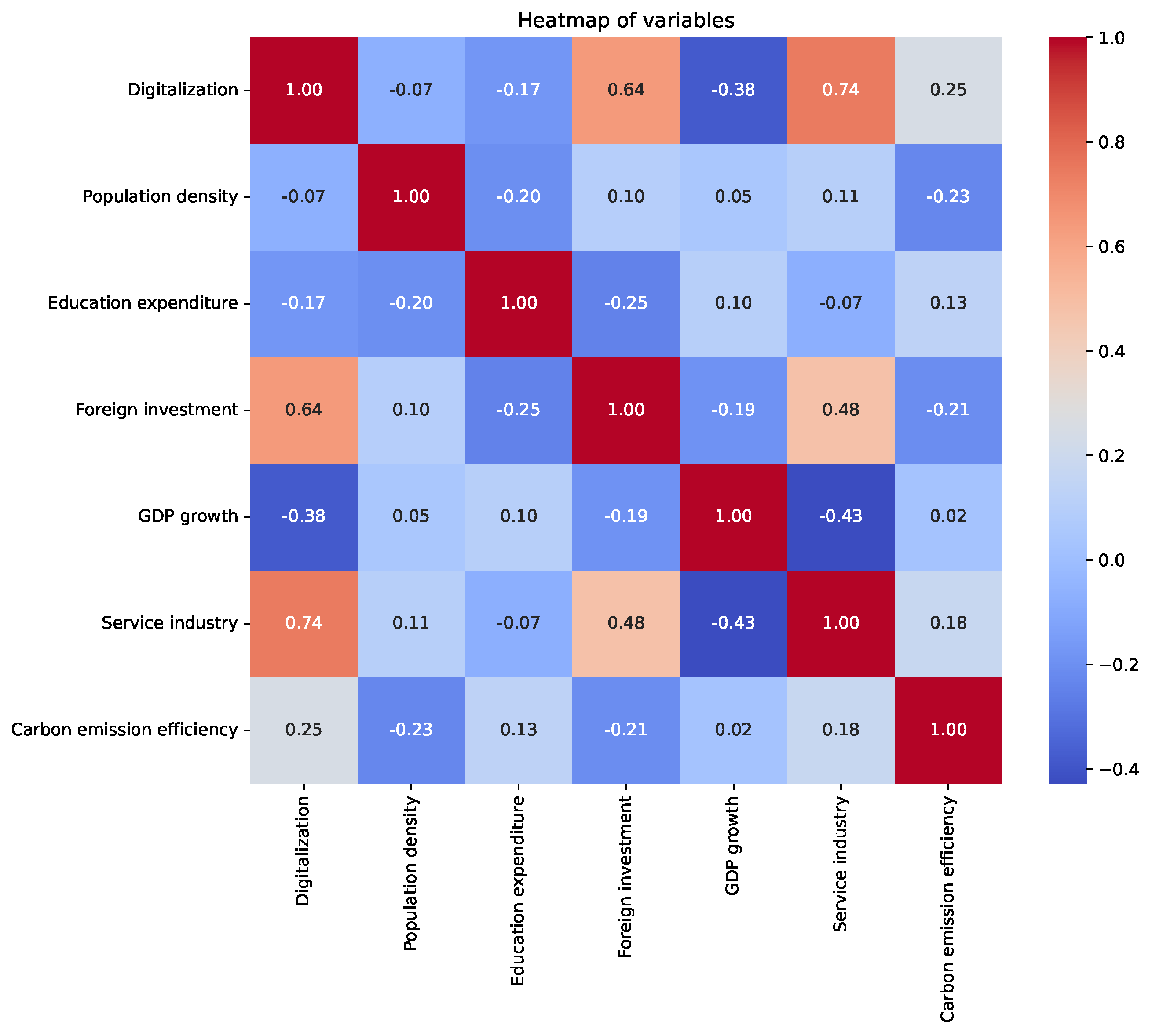
3.1. Variables and Data Sources

We construct a panel dataset to empirically analyze the impact of digitalization on carbon emission efficiency. The dataset covers a range of countries over recent years (specific years and country count are determined by data availability). Below we describe the key variables, their definitions, and data sources, in addition to the primary variables of interest: carbon emission efficiency and digitalization. We include several control variables that are commonly found to influence carbon efficiency, such as population density, education level, foreign investment, economic growth, and industrial structure.

Carbon Emission Efficiency [24]: A growing number of articles are examining the efficiency of carbon emissions in different countries, regions and industries, seeking ways to decouple carbon emissions from development. Panel data methods have become central to these studies because they allow researchers to control for unobserved heterogeneity between entities and observe the temporal dynamics of efficiency gains. By utilizing longitudinal data, analysts can determine not only the factors that influence carbon emission efficiency but also how these relationships have evolved over time. Both parametric and non-parametric frontier methods have employed to measure carbon emission efficiency by researches.The parametric Stochastic Frontier Analysis (SFA) models efficiency by combining error terms [25], while non-parametric Data Envelopment Analysis (DEA) constructs an efficiency frontier from input–output data without assuming a functional form. Traditional DEA models were extended to handle undesirable outputs like carbon by combining the concepts of weak disposability and relaxation-based measures [26]. Many recent studies use DEA-based models, especially SBM and its variants, to evaluate carbon emission efficiency across countries, regions, and sectors. For example, super-SBM DEA models have been applied to Chinese provinces and cities to evaluate carbon efficiency performance [27,28]. These studies often reveal significant regional differences; for example, economically developed regions tend to exhibit higher carbon emission efficiency than other regions [28,29]. Temporal trends are also observed; for instance, efficiency scores in most provinces show great improvement over time [27,28]. Sector-specific DEA analyses were further employed. The logistics industry has been evaluated using DEA/SBM models, generally showing moderate efficiency levels with room for improvement [30,31]. In the agricultural sector, DEA results indicate significant heterogeneity in carbon efficiency and highlight the trade-offs between agricultural output and carbon emissions [32,33]. The DEA/SFA frontier approach establishes a foundation for measuring carbon emission efficiency, finding that many regions and industries operate below the efficient frontier [29,34]. These efficiency scores provide the dependent variables for subsequent panel data analyses of driving factors.

Digitalization: Digitalization encompasses every aspect of social development and covers multiple fields, including finance, economy, and more. Contemporary studies increasingly examine the role of the digital economy and green finance in carbon emission efficiency, often using advanced panel data methods like mediation models, panel threshold models, and difference-in-differences. The digital economy—encompassing e-commerce, fintech, digital infrastructure—is generally found to boost carbon emission efficiency by promoting innovation and optimizing resource use [8,10,18,35]. For example, a provincial panel study shows that regions with higher digital finance development achieve better carbon efficiency, and this effect operates through two main channels: stimulating green technological innovation and expanding green financing options [18,35]. Similarly, growth in e-commerce and internet penetration has been linked to efficiency gains by improving market access for clean technologies and enabling smarter logistics [10]. Yu et al. note that while the digital economy improves carbon efficiency on average, it also helps correct industrial structure distortions, which further enhances efficiency [8]. Green finance is another pivotal factor, empirical evidence suggests a dual-threshold effect of green finance on efficiency—its positive impact becomes significant only after a certain level of economic development is reached and strengthens in wealthier regions [36]. This implies that green finance initiatives yield greater efficiency dividends in advanced economies or cities, whereas less developed regions might initially see limited effects. Nonetheless, as green finance grows (through instruments like green bonds, loans, and funds), it facilitates capital for clean energy and efficiency projects, thereby pushing the efficiency frontier outward [18].

Control Variables: This paper include a set of control variables that might affect carbon emission efficiency to isolate the specific effect of digitalization. The controls in the model are as follows:

Population Density (World Bank, people per square km of land area): Higher population density could have ambiguous effects on carbon efficiency. On one hand, denser areas may achieve economies of scale in public transport and infrastructure, potentially improving efficiency; on the other hand, they might also suffer from congestion and pollution concentration. In the data, population density ranges from about 1.25 to 7.16 (logarithmic units), with a mean of 4.35. We observe a weak negative correlation between population density and CEE, suggesting that very densely populated countries may face greater environmental pressures that lower efficiency.

Education Expenditure (World Bank, as a percentage of GDP, or a comparable index of education investment): Education levels can influence carbon efficiency through the development and adoption of cleaner technologies and practices. We include government education expenditure as a proxy for a country’s investment in human capital and knowledge. In the dataset, education expenditure varies widely, from about 5.26% to 32.59% of GDP, with a mean of 13.65%. Interestingly, we find that education expenditure is slightly negatively correlated with foreign investment in the sample, perhaps indicating that countries prioritizing internal development (education) might receive relatively less foreign capital or that some low-investment countries attract more foreign funds.

Foreign Investment (World Bank, net inflows of foreign direct investment, % of GDP): FDI can bring advanced technologies and management practices that improve energy and carbon efficiency (as noted in prior literature). We control for FDI (labeled as “foreign investment” in

Table 1. Variable description and summary statistics.

Variable	Description	Obs	Mean	Std	Min	Max
Digitization	DE index	1160	0.00086	0.00041	0.000058	0.0016
Population density	People per km2 of land area	1160	4.35	1.24	1.25	7.16
Education expenditure	Cost on education	1160	13.65	3.86	5.26	32.59
Foreign investment	Direct investment from foreign countries	1160	21.78	2.70	6.91	27.11
GDP growth	GDP growth annual	1160	3.33	3.27	−16.04	24.62
Industry	Services, value added (% of GDP)	1160	0.59	0.086	0.22	0.80
Carbon emission efficiency	CEE index	1160	0.39	0.14	0.18	1.67

) measured in relative terms. The sample shows FDI values between 6.91% and 27.11% of GDP, with an average of 21.78%. Digitalization shows a strong positive correlation with FDI, indicating that more digitalized countries tend to attract more foreign investment—possibly due to better business environments and infrastructure. This underscores how digitalization can make regions more attractive to investors.

GDP Growth (World Bank, annual % growth rate): Economic growth rates are included to capture cyclical or developmental effects. Rapid GDP growth might initially degrade efficiency if growth is powered by energy-intensive expansion, but over time growth often coincides with efficiency improvements (as economies mature and invest in cleaner technology). In the data, annual GDP growth ranges from –16.04% (deep recession) to 24.62% (fast expansion), with a mean of 3.33%. This wide range captures normal economic cycles as well as crises.

Industry Structure (World Bank, proxied by the share of the service sector in GDP): This paper uses the value added by services (% of GDP) as an indicator of a country’s industrial structure. A higher service sector share typically means a more post-industrial economy, which could correlate with higher carbon efficiency since services generally emit less CO₂ than heavy industry. In the sample, the service sector share (“industry” in Table 1, though it actually represents the service value-added fraction) ranges from 22% to 80%, with an average of 59%. We find that digitalization is strongly positively correlated with the service sector share. This suggests that highly digitalized economies are often service oriented, reflecting modern economic structures. We also note a negative correlation between service sector share and GDP growth, which might imply that in some developing countries, rapid growth is associated with industrial expansion, thus temporarily lowering the service share.

Table 1 summarizes the descriptive statistics for each variable. Notably, the standard deviation of the CEE index is $0.14$, highlighting significant variability in carbon emission efficiency across different countries. Education expenditure also varies widely, ranging from a minimum of $5.26$ to a maximum of $32.59$, reflecting substantial disparities in investment in education among nations. Additionally, the variable DE index exhibits large standard deviations, further suggesting notable differences in economic levels between the studied countries. Figure 1 shows the correlation coefficients between different variables. Digitalization exhibits a strong positive correlation with foreign investment, with a correlation coefficient of $0.64$, indicating that higher levels of digitalization may enhance the attractiveness of regions to foreign investors. This could be attributed to the better infrastructure and business environment typically found in areas with advanced digitalization. Additionally, digitalization shows a very strong positive correlation with the service industry, with a correlation coefficient of $0.74$. This suggests that the application of digital technologies can enhance service efficiency and drive innovation, thereby promoting the development of the service sector. Furthermore, foreign investment and the service industry are positively correlated with a coefficient of $0.48$, implying that foreign investment may contribute to the growth of the service industry by introducing advanced technologies and management practices. Meanwhile, population density and carbon emission efficiency show a weak negative correlation of $-0.23$, indicating that densely populated areas may face greater environmental pressures, potentially leading to lower carbon emission efficiency. Education expenditure and foreign investment exhibit a weak negative correlation of $-0.25$, which might suggest that regions with higher education spending could be less appealing to foreign investors, possibly due to differing priorities in resource allocation. The service industry and GDP growth are negatively correlated with a coefficient of $-0.43$, which might imply that the rapid development of the service sector could have a crowding-out effect on traditional industries or that the service sector’s contribution to GDP may be indirect. Lastly, carbon emission efficiency and foreign investment show a weak negative correlation of $-0.21$, suggesting that increased foreign investment might negatively impact carbon emission efficiency or that regions with higher carbon efficiency may be less attractive to foreign investors. These findings highlight the complex interplay between economic, environmental, and social factors and underscore the need for further research to explore the underlying causal mechanisms.

3.2. Data Pre-Processing

To simplify subsequent research processes, we preprocess the collected data. For the accuracy of the model, we calculate the skewness for each dataset, which reflects the degree of asymmetry in the data distribution. When the skewness is large, the data distribution significantly deviates from normality, potentially leading to inaccurate results from certain statistical methods. To address this issue, we set a threshold of 1. For datasets with skewness greater than 1, we apply a logarithmic transformation to normalize the data [37]. The formula for calculating skewness is as follows:

$$Skew={\displaystyle \frac{n}{(n-1)(n-2)}}\sum _{i=1}^n{\left({\displaystyle \frac{x_i-\overline{x}}{s}}\right)}^3$$

(1)

where n is the sample size, $x_i$ is the i-th sample observation, $\overline{x}$ is the sample mean, and s is the sample standard deviation.

For missing values, this paper adopts a multiple imputation method, which relies on the Multivariate Imputation by Chained Equations (MICE) algorithm. As a preparatory work, we initialize the imputation kernel and load the data to be imputed. Then, we conduct multiple iterative imputations. In each iteration, we sequentially build prediction models for variables with missing values, using other variables as independent variables to predict and replace the missing values. After reaching the specified number of iterations, we obtain the imputed data from the last iteration [38]. For the results, we combine the fixed columns that are not involved in the imputation process with the imputed data to form a complete dataset.

For the major independent variables, this paper assigns weights to the existing variables using the entropy weight method. The entropy weight method is an objective numerical technique used for assigning weights by applying entropy theory. It calculates the weights of indicators for various influencing factors without subjective bias, thereby objectively representing each factor’s significance in the comprehensive evaluation process [39]. The calculation steps of this method are as follows. Since all the indicators are positively oriented metrics. For subsequent processing, we standardize the data.

$$y_{ij}={\displaystyle \frac{x_{ij}}{{\sum }_{i=1}^m{x}_{ij}}},$$

(2)

where $x_{ij}$ is the value of the i-th sample under the j-th indicator, and $y_{ij}$ is the standardized value. Using the calculation formula of the entropy weight method, we calculate the entropy values of the indicators.

$$e_j=-k\sum _{i=1}^m{p}_{ij}ln\left(p_{ij}\right)$$

(3)

where $p_{ij}={\displaystyle \frac{y_{ij}}{{\sum }_{i=1}^m{y}_{ij}}}$, $k={\displaystyle \frac{1}{ln\left(m\right)}}$, and m is the number of samples. Because a smaller information entropy indicates that the indicator is more important, we compute the difference coefficients of the indicators:

$$g_j=1-e_j.$$

(4)

As a result, we derive the weights of the indicators:

$$w_j={\displaystyle \frac{g_j}{{\sum }_{j=1}^n{g}_j}}.$$

(5)

3.3. Model Setting

Having prepared the data, we now introduce the intrinsic Gaussian Process Regression (iGPR) model, which forms the core of the methodological innovation. The iGPR is essentially a regression model that combines traditional fixed effects (for observable covariates) with a Gaussian process (GP) prior to model spatial random effects intrinsic to non-Euclidean covariate spaces (such as coordinates on a sphere or other manifold). This allows us to capture complex spatial patterns in the relationship between digitalization and carbon efficiency. K-dimensional Euclidean covariates $\mathit{x}$ and covariates $\delta \left(\mathit{s}\right)$ from non-Euclidean spaces, which represent the spatial position, are assumed to exhibit a nonlinear relationship with Y. The model can be expressed as follows:

$$Y=f\left(\mathit{x}\right)+\delta \left(\mathit{s}\right)$$

(6)

where $Y\in \mathcal{R}$ is a scalar and $\mathit{x}=(x_1,x_2,\dots ,x_K)\in {\mathcal{R}}^K$. The function $f\left(\mathit{x}\right)$ is considered to obey Gaussian distribution.

$$f\left(\mathit{x}\right)\sim \mathcal{GP}\left(\mathbb{E}\left[f\left(\mathit{x}\right)\right],k_{\theta }\left(\mathit{x},{\mathit{x}}^{\prime }\right)\right),$$

(7)

where $\mathbb{E}\left[f\right(\mathit{x}\left)\right]$ is the mean function of $f\left(\mathit{x}\right)$ and $k_{\theta }\left(\mathit{x},{\mathit{x}}^{\prime }\right)=\mathbb{E}\left[\left(f\left(\mathit{x}\right)-\mathbb{E}\left(\mathit{x}\right)\right){\left(f\left(\mathit{x}\right)-\mathbb{E}\left(\mathit{x}\right)\right)}^{\top }\right]$ is the covariance function, which can be denoted by some kernel functions, such as the RBF kernel, Dot Product kernel, White kernel and Gaussian kernel. The function $\delta \left(\mathit{s}\right)$ is considered as the random effects, where $\mathit{s}$ is from a non-Euclidean manifold. We employ a Reproducing Kernel-Based method [40] to model on the manifold, i.e.,

$$\delta \left(\mathit{s}\right)=\sum _{j=1}^{\infty }{\eta }_j{k}_{\sigma }\left(\mathit{s},{\mathit{s}}^{\prime }\right),$$

(8)

where $k_{\sigma }\left(\mathit{s},{\mathit{s}}^{\prime }\right)$ is the kernel function and ${\eta }_j,j=1,2,\cdots$ is the coefficient corresponding to the kernel function. For the above infinite series, we adopt the Karhunen–Loève truncation to iteratively compute a finite number of terms in practice.The covariance matrix $\mathbf{C}$ of the dataset $\{{\mathit{x}}_1,{\mathit{x}}_2,\dots ,{\mathit{x}}_N\}$ is computed as

$$\mathbf{C}={\displaystyle \frac{1}{N-1}}\sum _{i=1}^N({\mathit{x}}_i-\mu ){({\mathit{x}}_i-\mu )}^T$$

(9)

where $\mu ={\displaystyle \frac{1}{N}}{\sum }_{i=1}^N{\mathit{x}}_i$ is the mean vector.

Performing eigen decomposition on $\mathbf{C}$ yields

$$\mathbf{C}=\mathbf{U}\mathbf{\Lambda }{\mathbf{U}}^T$$

(10)

where $\mathbf{U}=[{\mathit{u}}_1,{\mathit{u}}_2,\dots ,{\mathit{u}}_n]$ contains the eigenvectors and $\mathbf{\Lambda }=\mathrm{diag}({\lambda }_1,{\lambda }_2,\dots ,{\lambda }_n)$ with ${\lambda }_1\ge {\lambda }_2\ge \cdots \ge {\lambda }_n\ge 0$.

The truncation dimension k is determined by the cumulative variance ratio.

$${\displaystyle \frac{{\sum }_{i=1}^k{\lambda }_i}{{\sum }_{i=1}^n{\lambda }_i}}\ge \alpha$$

(11)

A typical value for $\alpha$ is $0.95$.

The transformation matrix ${\mathbf{U}}_k$ is formed by the first k eigenvectors.

$${\mathbf{U}}_k=[{\mathbf{u}}_1,{\mathbf{u}}_2,\dots ,{\mathbf{u}}_k]\in {\mathbb{R}}^{n\times k}$$

(12)

The original data $\mathbf{X}\in {\mathbb{R}}^{N\times n}$ is projected to the low-dimensional space

$${\mathbf{Y}}_k=\mathbf{X}{\mathbf{U}}_k\in {\mathbb{R}}^{N\times k}$$

(13)

The reconstructed data in the original space is

$$\widehat{\mathbf{X}}={\mathbf{Y}}_k{\mathbf{U}}_k^T=\mathbf{X}{\mathbf{U}}_k{\mathbf{U}}_k^T$$

(14)

Under these assumptions, the response satisfies a Gaussian process prior:

$$Y\sim \mathcal{GP}\left(\sum _{j=1}^{\infty }{\eta }_j{k}_{\sigma }\left(\mathit{s},{\mathit{s}}^{\prime }\right)+\mathbb{E}\left[f\left(\mathit{x}\right)\right],k_{\theta }\left(\mathit{x},{\mathit{x}}^{\prime }\right)\right).$$

(15)

where $k_{\tau }(s,s^{\prime })$ represents the Gaussian kernel function, while $k_{\theta }(x,x^{\prime })$ represents the covariance structure of Gaussian processes in feature space. In summary, this paper proposes the above model; we name it the intrinsic Gaussian Process Regression (iGPR) model, and we will explain the estimation process of the slope parameter $\eta$, the kernel parameter of the random effect $\sigma$, and the kernel parameter of GP in the next section.

3.4. Parameter Estimation

This paper will demonstrate parameter estimation with sample data in this section. To incorporate the manifold’s nonlinear geometry in the model, we adopt a kernel-based approach using the heat kernel on $\mathcal{M}$. The heat kernel $p_t(x,y)$ intrinsically captures the structure of the data on the manifold—it can be viewed as the analog of a Gaussian kernel in the non-Euclidean space $\mathcal{M}$. Mathematically, $p_t(x,y)$ is the fundamental solution of the heat equation on $\mathcal{M}$; equivalently, it represents the transition probability density of a Brownian motion on $\mathcal{M}$ from starting point x to endpoint y in time t. Rather than attempting a closed-form solution for $p_t(x,y)$, we estimate the heat kernel by simulating Brownian motion on the manifold. The basic idea is to perform a Monte Carlo simulation of many random walks on $\mathcal{M}$ and use their endpoint distribution to approximate $p_t(x,·)$. In practice, we simulate the Brownian motion as a stochastic differential equation (SDE) evolving on $\mathcal{M}$ via small time steps. Because $\mathcal{M}$ is non-Euclidean, we use a local parameterization to approximate each small step in Euclidean space. Specifically, at the current position $X_t\in \mathcal{M}$, we choose a local coordinate chart $\varphi$ that maps a neighborhood of $X_t$ on the manifold to an open set in Euclidean space. We can think of $\varphi \left(X_t\right)\in {\mathbb{R}}^d$ (with $d=dim\mathcal{M}$) as the coordinate representation of $X_t$. If the manifold is embedded in ${\mathbb{R}}^{d_e}$ (with $d_e\ge d$), this local coordinate can be viewed as an embedded Euclidean coordinate system around $X_t$. In these coordinates, the infinitesimal dynamics of a Brownian particle are approximately those of a standard Brownian motion in Euclidean space. We therefore consider the SDE (in Itô form) for the coordinate process $Y_t=\varphi \left(X_t\right)$.

$$d{Y}_t=d{W}_t,$$

(16)

where $W_t$ is a standard Brownian motion in the appropriate Euclidean space (of dimension dd or $d_e$, as appropriate). This SDE simply says that, in local Euclidean coordinates, the point undergoes a random Gaussian displacement with no drift. Consequently, over an infinitesimal time h, the transition of $Y_t$ is given by a Gaussian distribution. In fact, for a small time step h, the transition probability density for moving from $Y_t=u$ to $Y_{t+h}=v$ is

$$p_h^{\left(\mathrm{Euclid}\right)}(u,v)={\displaystyle \frac{1}{{\left(2\pi h\right)}^{d/2}}}exp\left(-{\displaystyle \frac{{\parallel v-u\parallel }^2}{2h}}\right),$$

(17)

which is the Gaussian heat kernel in ${\mathbb{R}}^d$. Mapping this back to the manifold via $u=\varphi \left(x\right)$ and $v=\varphi \left(y\right)$, we obtain an approximate transition density on $\mathcal{M}$ for small time h. Repeating such small transitions allows us to simulate the Brownian motion on $\mathcal{M}$. We use a Euler–Maruyama discretization of the SDE to generate the sample paths. In discrete form, if we use a time step $h=t/K$ (with K steps to reach time t), the update rule is

$$Y_{n+1}=Y_n+\sqrt{h}{\xi }_n,{\xi }_n\sim \mathcal{N}(0,I)$$

(18)

where ${\xi }_n$ is a random Gaussian vector (of the same dimension as Y) with zero mean and identity covariance. Each increment $\sqrt{h},{\xi }_n$ is a realization of the infinitesimal Brownian motion over time h. After computing $Y_{n+1}$ in the local coordinates, we map it back to the manifold: $X_{n+1}={\varphi }^{-1}\left(Y_{n+1}\right)$. This ensures that $X_{n+1}\in \mathcal{M}$; i.e., the step stays on the manifold. Starting from an initial point $X_0=x$ and applying the update formula iteratively, we obtain a discrete Brownian trajectory $X_0,X_h,X_{2h},\dots ,X_t$ on the manifold. By construction, in the limit $h\to 0$, this trajectory converges to a true Brownian motion on $\mathcal{M}$.

We repeat this simulation many times to build an empirical estimate of the heat kernel. After N independent random walks of duration t (each starting at x), we have endpoints $X_t^{\left(1\right)},X_t^{\left(2\right)},\dots ,X_t^{\left(N\right)}$, which are approximately distributed according to $p_t(x,·)$. The heat kernel value $p_t(x,y)$ can then be estimated, for example, by counting the fraction of endpoints that fall inside a small neighborhood of y (or by density estimation techniques on the samples). This stochastic algorithm converges to the true heat kernel as the simulation parameters are refined. In particular, as the step size $h\to 0$, the discrete random walk approaches the continuous Brownian motion on $\mathcal{M}$, eliminating time-discretization bias. Meanwhile, as the number of simulations $N\to \infty$, the Monte Carlo sampling error vanishes by the law of large numbers. More concretely, for smooth enough $\mathcal{M}$, one can show that the heat kernel estimator is consistent and the mean squared error decays on the order of $h^2+{\displaystyle \frac{1}{N}}$. In other words, the bias is $O\left(h\right)$ (first order in the time step) and the variance is $O(1/N)$, so the combined error can be made arbitrarily small by choosing h sufficiently small and N sufficiently large. This ensures that the kernel approximation $p_t(x,y)$ can be as accurate as needed while inherently accounting for the manifold’s nonlinear geometry through the use of the heat kernel.

For the sake of simplicity in description, we have rewritten the proposed model in the following form:

$$Y=f\left(x\right)+A^{T}B$$

(19)

Consider the latent link function $R_e(·)$ that relates inputs to the response. For n observed data points ${(X_i,{\delta }_i,Y_i)}_{i=1}^n$ (where $X_i$ represents Euclidean covariates and ${\delta }_i$ represents random effect for observation i), we assume the finite-sample realization of $R_e$ follows a multivariate Gaussian prior. In particular, the vector of link function values at the observed inputs is modeled as a normal distribution.

$$\left(R_e(A_1,{\delta }_1),R_e(A_2,{\delta }_2),\dots ,R_e(A_n,{\delta }_n)\right)\sim \mathcal{N}\left(\mathbf{V},{\mathit{K}}_{\mathit{\theta }}\right),$$

(20)

where $\mathbf{V}$ is the prior mean vector and $\mathit{K}\ast \mathit{\theta }$ is the $n\times n$ kernel (covariance) matrix. The $(i,i^{\prime })$-th entry of $\mathit{K}\ast \mathit{\theta }$ is given by $k_{\mathit{\theta }}(S_i,S_{i^{\prime }})$, the chosen kernel function evaluated at the covariate information of observations i and $i^{\prime }$. (In the model, $\mathbf{V}$ captures the contribution of fixed effects, e.g., through the truncated Karhunen–Loève expansion of functional covariates, and $A_i$ denotes the vector of basis coefficients for observation i.) This Gaussian process prior on the link function introduces a flexible random effect in the regression model.

The model parameters are learned within a Penalized Maximum-Likelihood Estimation (PMLE) framework. Specifically, we construct a likelihood function for the observed responses $\mathbf{Y}={(Y_1,\dots ,Y_n)}^{\top }$ under the model. Let $\mathit{B}=(b_1^{\top },b_2^{\top },\dots ,b_J^{\top })$ collect the coefficient vectors $b_j$ for the basis expansion of the functional slope functions, and let $\mathit{\theta }$ denote the hyperparameters of the covariance kernel. The *marginal likelihood* of the data (integrating over the Gaussian process random effect) is given by the following equation. In simplified form, this likelihood can be expressed as

$$L(\mathit{B},{\sigma }^2,\mathit{\theta })={\displaystyle \frac{1}{\sqrt{{\left(2\pi {\sigma }^2\right)}^{n/2}\left|{\mathit{K}}_{\mathit{\theta }}\right|}}}\exp \left(-{\displaystyle \frac{1}{2}}{\displaystyle \frac{{(\mathit{Y}-{\mathit{A}}^{\top }\mathit{B})}^{\top }{\mathit{K}}_{\mathit{\theta }}^{-1}(\mathit{Y}-{\mathit{A}}^{\top }\mathit{B})}{{\sigma }^2}}\right),$$

(21)

where $A={(A_1^{\top },A_2^{\top },\dots ,A_n^{\top })}^{\top }$ is the $n\times J$ matrix of basis coefficients (each $A_i$ corresponds to observation i), ${\sigma }^2$ is the observation noise variance, and $|{\mathit{K}}_{\mathit{\theta }}|$ denotes the determinant of the kernel covariance matrix. To facilitate optimization, we maximize the log-likelihood; equivalently, we minimize the negative log-likelihood augmented with an $L_2$ regularization term on the coefficient vectors $b_j$. This yields a convex loss function defined in the following equation:

$$-ln\left(L(\mathit{B},{\sigma }^2,\mathit{\theta })\right):={\displaystyle \frac{1}{2{\sigma }^2}}{(\mathit{Y}-{\mathit{A}}^{\top }\mathit{B})}^{\top }{\mathit{K}}_{\mathit{\theta }}^{-1}(\mathit{Y}-{\mathit{A}}^{\top }\mathit{B})+nln\left({\sigma }^2\right)+ln\left(\right|{\mathit{K}}_{\mathit{\theta }}\left|\right)+\lambda \sum _{j=1}^J{\parallel {\mathit{B}}_j\parallel }_2^2$$

(22)

where $\lambda$ is a regularization hyperparameter and $|·|\ast 2$ denotes the Euclidean norm. The quadratic penalty $\lambda \sum \ast j|b_j{|}_2^2$ serves to constrain the magnitude of the slope function coefficients $b_j$, thereby preventing overfitting (over-parameterization) of the functional effect.

We employ a quasi-Newton solver, L-BFGS-S, to efficiently minimize the objective function. This algorithm approximates the Hessian matrix and handles high-dimensional parameter spaces while allowing bound constraints on parameters. In contrast to stochastic gradient descent (SGD), the L-BFGS-S method does not require manual tuning of a learning rate and is more robust even for non-smooth objectives. This makes it well suited for jointly optimizing continuous variables (like $\mathit{\theta }$) and discrete variables (such as the truncation level Q for the functional basis) in the model. Moreover, the PMLE approach (using a fixed penalization) sidesteps the need for full Bayesian posterior sampling, thus avoiding the heavy computational cost of techniques like MCMC. After optimization, let $\widehat{\mathit{B}}$ and $\widehat{\mathit{\theta }}$ denote the estimated model parameters (at the attained local optimum of the loss). In the model, we use a squared exponential kernel augmented with additional components to capture different patterns in the data. The covariance function is defined as a combination of a linear kernel, a radial basis function (RBF) kernel, and a white noise term. In particular, we define

$$k_{\mathit{\theta }}(\mathit{x},{\mathit{x}}^{\prime })=\alpha x^{\top }x{S}^{\prime }exp\left(-{\displaystyle \frac{\parallel \mathit{x}-{\mathit{xS}}^{\prime }{\parallel }^2}{2h^2}}\right)+(1-\alpha )\delta (\mathit{x},{\mathit{x}}^{\prime }),$$

(23)

where $\mathit{\theta }=(\alpha ,h)$. Here $|x-x^{\prime }{|}^2$ is the squared Euclidean distance between two input feature vectors x and $x^{\prime }$, and $\delta (x,x^{\prime })$ is the Kronecker delta (which equals 1 if $x=x^{\prime }$ and 0 otherwise). The parameter $\alpha$ (with $0\le \alpha \le 1$) controls the relative weight of the signal components and effectively represents the noise variance in this formulation. In this composite kernel, the linear term $x^{\top }{x}^{\prime }$ captures any linear dependence on the covariates, the RBF (squared exponential) term $exp(-|x-x^{\prime }{|}^2/\left(2h^2\right))$ captures smooth nonlinear relationships (with h as the length-scale or bandwidth parameter), and the white noise term $\delta (x,x^{\prime })$ accounts for independent observational noise. By combining these components, the model can simultaneously represent linear trends, nonlinear effects, and noise in the data, which enhances its flexibility and robustness. We ensure that the combined kernel satisfies Mercer’s condition (closure under valid kernel operations), so it defines a proper covariance function for the Gaussian process prior.

After training, the proposed model can make predictions for new inputs by deriving the posterior predictive distribution from the Gaussian process. Consider a new test point with covariates $X^{*}, x^{*}$. Let $Y^{*}$ denote the (unknown) response at this test point, and let ${\widehat{\gamma }}^2$ be the estimated noise variance (corresponding to ${\sigma }^2$ or related to $1-\widehat{\alpha }$ in the kernel). We first write the joint distribution of the observed outputs and the test output, incorporating the covariance structure and the mean contributions from the fixed effects. The joint distribution of $\mathbf{Y}$ (the $n\times 1$ training output vector) and $Y^{*}$ is given by a multivariate normal:

$$\left(\begin{array}{c}\mathit{Y}\\ Y^{*}\end{array}\right)\sim \mathcal{N}\left(\left(\begin{array}{c}{\mathit{A}}^{\top }\widehat{\mathit{B}}\\ {\mathit{A}}^{*\top }\widehat{\mathit{B}}\end{array}\right),\left(\begin{array}{cc}{\mathit{K}}_{\widehat{\mathit{\theta }}}(\mathit{x},{\mathit{x}}^{\prime })+{\gamma }^{2}I& {\mathit{K}}_{\widehat{\mathit{\theta }}}({\mathit{x}}^{*},\mathit{x})\\ {\mathit{K}}_{\widehat{\mathit{\theta }}}^{\top }({\mathit{x}}^{*},\mathit{x})& k_{\widehat{\mathit{\theta }}}({\mathit{x}}^{*},{\mathit{x}}^{*})\end{array}\right)\right)$$

(24)

where $A^{*}=(a_1^{*},a_2^{*},\dots ,a_J^{*})$ represents the vector of basis coefficients for the functional covariates at the test point (analogous to each $A_i$ for training data), and I is the $n\times n$ identity matrix. The top-left block of the covariance matrix is the training data covariance (with noise ${\widehat{\gamma }}^2$ on the diagonal), the top-right block ${\mathit{K}}_{\mathit{\theta }}(x,x^{*})$ is the $n\times 1$ covariance vector between each training point and the test point, and the bottom-right term $K_{\mathit{\theta }}(x^{*},x^{*})$ is the variance at the test point. The mean vector has two components: $A^{\top }\widehat{\mathit{B}}$ is the length-n vector of mean outputs for the training data (from the fixed-effect part of the model), and ${A^{*}}^{\top }\widehat{\mathit{B}}$ is the corresponding mean contribution for the test input. Using Bayesian Gaussian process inference conditioned on the observed training data, the predictive distribution for $Y^{*}$ can be derived analytically. It is also Gaussian, with a closed-form mean and variance. In fact, conditioning the joint normal on $\mathbf{Y}$ yields

$$Y^{*}|{\{{\mathit{X}}_i.{\delta }_i,Y_i\}}_{i=1}^n,\{{\mathit{X}}^{*},{\delta }^{*}\},\widehat{\mathit{B}},\widehat{\mathit{\theta }}$$

$$\sim \mathcal{N}({\mathit{A}}^{*\top }\widehat{\mathit{B}}+{\mathit{K}}_{\widehat{\mathit{\theta }}}^{*\top }{({\mathit{K}}_{\widehat{\mathit{\theta }}}+{\gamma }^{2}I)}^{-1}(\mathit{Y}-{\mathit{A}}^{\top }\widehat{\mathit{B}}),k_{\widehat{\mathit{\theta }}}+{\mathit{K}}_{\widehat{\mathit{\theta }}}^{*\top }{({\mathit{K}}_{\widehat{\mathit{\theta }}}+{\gamma }^{2}I)}^{-1}{\mathit{K}}_{\widehat{\mathit{\theta }}}^{*})$$

(25)

where we use the shorthand ${\mathit{K}}^{*}:={\mathit{K}}_{\mathit{\theta }}^{*}(x,x^{*})$ for the $n\times 1$ covariance vector between the n training points and the test point. The mean of this predictive distribution (the first term inside the $\mathcal{N}(·,·)$ above) consists of two parts: ${A^{*}}^{\top }\widehat{\mathit{B}}$ is the predicted contribution from the functional linear component, and ${\mathit{K}}^{*\top }{({\mathit{K}}_{\mathit{\theta }}^{*}+{\widehat{\gamma }}^{2}I)}^{-1}(\mathit{Y}-A^{\top }\widehat{\mathit{B}})$ is the contribution from the Gaussian process random effect (essentially a kernel-weighted interpolation of the residuals). The variance (second term) equals the prior variance at $x^{*}$ plus noise ${\widehat{\gamma }}^2$ minus the covariance terms, in accordance with Gaussian process posterior variance formula. For point prediction, we can use the maximum a posteriori (MAP) estimate of $Y^{*}$ given this predictive distribution. Since the predictive distribution is Gaussian, the MAP estimate is simply its mean. Thus, the predictive mean serves as the regression estimate for the new input. This predicted value (conditional mean) is given by the follow equation:

$${\widehat{Y}}^{*}={\mathit{A}}^{*\top }\widehat{\mathit{B}}+{\mathit{K}}_{\widehat{\mathit{\theta }}}^{*\top }{\mathit{K}}_{\widehat{\mathit{\theta }}}^{-1}(\mathit{Y}-{\mathit{A}}^{\top }\widehat{\mathit{B}}).$$

(26)

which is the sum of the fixed-effect prediction and the Gaussian process update term.

The most computationally intensive operations in each likelihood evaluation are the inversion of the $n\times n$ covariance matrix $K_{\theta }$ (or solving linear systems involving it) and the determinant calculation, which are on the order of $O\left(n^3\right)$ in naive implementation. For $n\approx 1160$, this is manageable on a modern computer. However, if n were much larger (e.g., tens of thousands), naive GP inference would become impractical. In that case, one might consider sparse GP approximations or iterative methods to approximate $K_{\theta }^{-1}$, as well as exploiting structure in the covariance (like using inducing points or low-rank approximations). In the study, because of the moderate sample size and the use of efficient linear algebra routines, the optimization was tractable. We also mitigate complexity by the aforementioned truncation of the spatial basis (reducing J) and by possibly batching the computation of the heat kernel via Monte Carlo (which we discuss next). Overall, the algorithm scales on the order of $O\left(n^3\right)$ for the GP part, plus the cost of the Monte Carlo simulation for the heat kernel which is polynomial in the number of simulation steps and particles but parallelizable. The derivation steps and a comprehensive pseudocode algorithm for the iGPR model are given in Appendix A.

4. Results and Discussion

4.1. Baseline Results

Each individual forecast ${\widehat{Y}}_i^{*}$ of i is given by ${\widehat{Y}}_i^{*}=A_i^{\top }\widehat{B}+K{i,\widehat{\theta }}^{\top }K\ast {\widehat{\theta }}^{-1}(Y-A^{\top }\widehat{B})$. As a result, the calculation of ATE is

$$\mathrm{ATE}={\displaystyle \frac{1}{n}}\sum _{i=1}^n({\widehat{Y}}_i-Y_i),$$

where ${\widehat{Y}}_i$ and $Y_i$ are for the first i, and the predicted values and real values n are for the sample size. ATE represents the average effect difference between the treatment group and the control group, that is, the average deviation between the model’s predicted values and the actual observed values. Through the calculation, we find that the ATE is about 0.00895, which is greater than 0. This means the predicted results (treatment group) have a positive impact on the outcome variable compared to the control group (true values), proving the high accuracy of the predictions.

As can be seen from

Table 2. MSE performance comparison across models.

	Mean	Std
iGPR	0.0047	0.0025
XGBoost	0.0082	0.0028
RF	0.0078	0.0026
SVR	0.1066	0.0327
ElasticNet	0.0226	0.0040
GPR	0.1479	0.0277

, the proposed iGPR algorithm shows significant reductions in MSE compared to traditional machine learning algorithms such as SVR and XGBoost. This achievement stems from the algorithm’s innovative hierarchical hybrid modeling architecture: At the foundational level, vectorized Haversine distance calculations and Gaussian kernel transformations convert raw geographic coordinates into spatially meaningful feature matrices with clear physical interpretations. The intermediate layer explicitly models spatial dependencies through L2-regularized linear components while simultaneously capturing complex nonlinear feature interactions via customized composite kernel functions. At the optimization level, the novel joint objective function unifies the regularization of spatial coefficients with Gaussian process marginal likelihood under an L-BFGS-B framework; this co-optimization mechanism not only avoids error accumulation inherent in traditional two-stage methods but also enhances model generalizability through parameter sharing. Figure 2 shows a histogram of residuals along with a fitted density curve. The residuals were found to lie mostly in the range –0.2 to 0.2, centered very tightly around 0, and approximately normally distributed. This indicates that the model’s errors are unbiased (centered at zero) and do not display heavy tails or skewness, and there are no signs of significant outliers or systematic under/over-prediction for certain ranges of data. Such an error distribution is consistent with a well-specified model and supports the validity of using Gaussian process assumptions (which imply normally distributed residuals if the model is capturing the structure correctly). The lack of large outliers also suggests that no individual data points are poorly explained, which can be attributed to the model’s flexibility and the effectiveness of the data preprocessing (the log transformations likely helped in preventing outliers due to skewed variables).

4.2. Robustness Checks

Robustness refers to the ability of a deep learning model to perform consistently and accurately when used with a wide range of input data, including data that may be noisy, incomplete, or confounded by various sources of interference [41]. Quantile regression is employed [42], which is useful for conducting robustness checks. The quantile regression model is established as follows:

$$Q_{\tau }\left(Y\right|X)=\mathbf{X}\beta$$

(27)

where $Q_{\tau }\left(Y\right|X)$ is the $\tau$-th quantile of Y given X. $\mathbf{X}$ is an $n\times p$ design matrix, where each row represents the independent variables of an observation. $\beta$ is a p-dimensional vector of regression coefficients. And then, the objective of the regression is to minimize the quantile loss function:

$${\rho }_{\tau }\left(u_i\right)=\tau ·max(y_i-{\mathbf{x}}_i^T\beta ,0)+(1-\tau )·max({\mathbf{x}}_i^T\beta -y_i,0)$$

(28)

The objective function of quantile regression is the sum of the loss functions for all observations:

$$\underset{\beta }{min}\sum _{i=1}^n{\rho }_{\tau }(y_i-{\mathbf{x}}_i^T\beta )$$

(29)

Expanding this summation form,

$$\underset{\beta }{min}\sum _{i=1}^n[\tau ·max(y_i-{\mathbf{x}}_i^T\beta ,0)+(1-\tau )·max({\mathbf{x}}_i^T\beta -y_i,0)]$$

(30)

The quantiles are set as $0.1$, $0.25$, $0.5$, $0.75$, $0.9$.

Table 3. Quantile regression results for robustness check.

Quantile	Parameter	Std Err	T-Stat	p-Value
0.1	0.2000	0.073	2.752	0.006
0.25	0.2383	0.105	2.269	0.024
0.5	0.2612	0.035	7.496	0.001
0.75	0.2685	0.036	7.390	0.001
0.9	0.2705	0.040	6.755	0.001

shows that when performing quantile regression, if the regression coefficients are statistically significant and consistent in direction across different quantiles, it indicates that the impact of the independent variable on the dependent variable is robust and not influenced by the distribution’s position.

4.3. Endogeneity Test

The Generalized Method of Moments addresses endogeneity by using instruments [43]. And the consistency and asymptotic normality of its estimator have been proven [44]. Considering the simple linear regression model

$$y=X\beta +u,$$

(31)

where y is the dependent variable, X is the matrix of explanatory variables that includes endogenous variables, $\beta$ is the vector of parameters to be estimated, and u is the error term. Next, we need to identify the endogenous variables, which are the variables correlated with the error term u. To address this issue, instrumental variables that are highly correlated with the endogenous variables and not correlated with the error term need to be found. That is, $E\left[Z^{\prime }u\right]=0$, where Z is the matrix containing the instrumental variables. For measuring the discrepancy between the sample moments and the theoretical moment conditions, an objective function is defined:

$$Q\left(\beta \right)={(y-X\beta )}^{\prime }W(y-X\beta ),$$

(32)

where W is the weighting matrix, chosen to be the inverse of $X^{\prime }X$ GMM estimation typically involves a two-step estimation process. The first step is to estimate the parameters using ordinary least squares (OLS). The second step is to use the estimates of the first step to optimize the objective function $Q\left(\beta \right)$ and obtain consistent parameter estimates.

For the GMM method, selecting appropriate instrumental variables (IVs) to ensure their exogeneity and the significance of the model is crucial. Therefore, we calculated the correlation coefficients between each candidate variable and both the endogenous variable and the dependent variable. We ultimately selected two indicators that exhibited strong correlation with the endogenous variable but weak correlation with the dependent variable as the instrumental variables. The descriptive statistics of these selected IVs are shown as

Table 4. Instrumental variable description and summary statistics for endogeneity check.

Variable	Obs	Mean	Std	Min	Max	Corr(DV)	Corr(EV)
working-age population ratio	1160	4.19	0.07	3.92	4.31	−0.015	0.501
Research expenditure	1160	1.3	1.05	0.005	5.22	0.008	0.75

.

Corr(DV) and Corr(EV) in Table 4 denote the correlation coefficients with the dependent variable (carbon emission efficiency) and endogenous variable (digitalization), respectively. Using these two sets of instrumental variables, we obtain the GMM estimation results, shown as

Table 5. Parameter estimation results using GMM.

Variable	Type	Parameter	Std Err	T-Stat	p-Value
Digitalization	endogenous	0.1913	0.0618	3.0925	0.0020
Population density	control	−0.2339	0.0183	−12.779	0.0000
Foreign investment	control	−0.1794	0.0319	−5.6220	0.0000
GDP growth	control	0.0661	0.0186	3.5496	0.0004

.

Table 4 presents the descriptive statistics of instrumental variables (IVs) used for the Generalized Method of Moments (GMM) analysis, specifically the working-age population ratio and research expenditure. These IVs were selected because they exhibit strong correlation with digitalization (the endogenous variable) and weak correlation with carbon emission efficiency (the dependent variable), thus meeting the exogeneity requirement for valid GMM estimation. Table 5 presents variable types (endogenous or control variables), estimated parameters from GMM regression, standard errors, t-statistics, and p-values. With all p-values being statistically significant (p < 0.05), the results demonstrate that all parameters are significantly different from zero. The model shows strong overall significance, indicating successful mitigation of endogeneity concerns.

Additionally, we need to use the Hansen-J test statistic to check whether the instrumental variables are over-identified [44]. The test statistic is as follows:

$$J=N·R^2,$$

(33)

where N is the number of observations, and $R^2$ is the squared correlation between the residuals from the regression of the instruments on the endogenous variables and the residuals from the original regression model. The null hypothesis of the Hansen-J test is that all instrumental variables are exogenous. In the model, the Hansen-J test statistic is $0.4803$ with a p-value of $0.4883$ (>$0.05$), failing to reject the null hypothesis. This suggests the instruments satisfy the exogeneity requirement for valid GMM estimation.

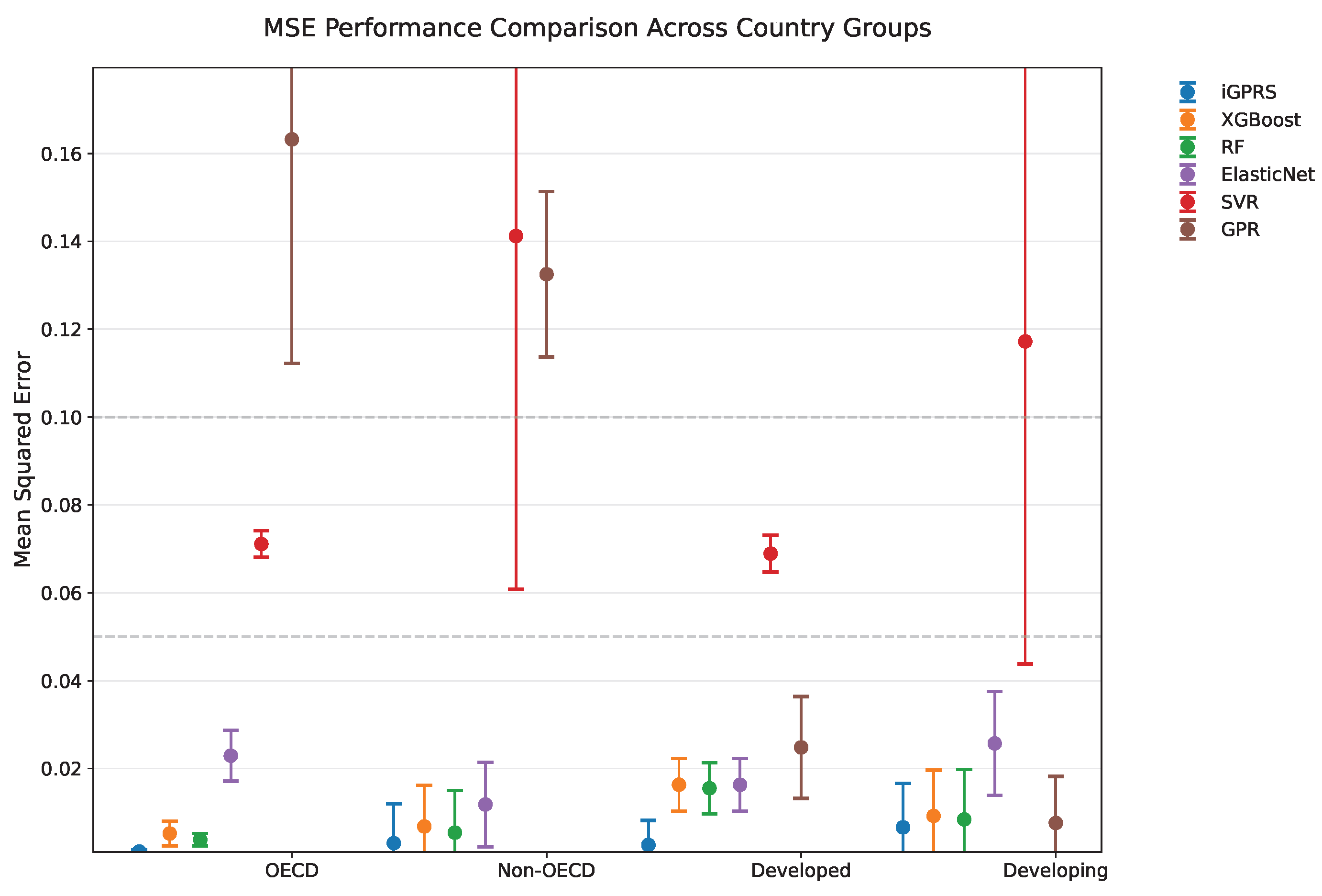
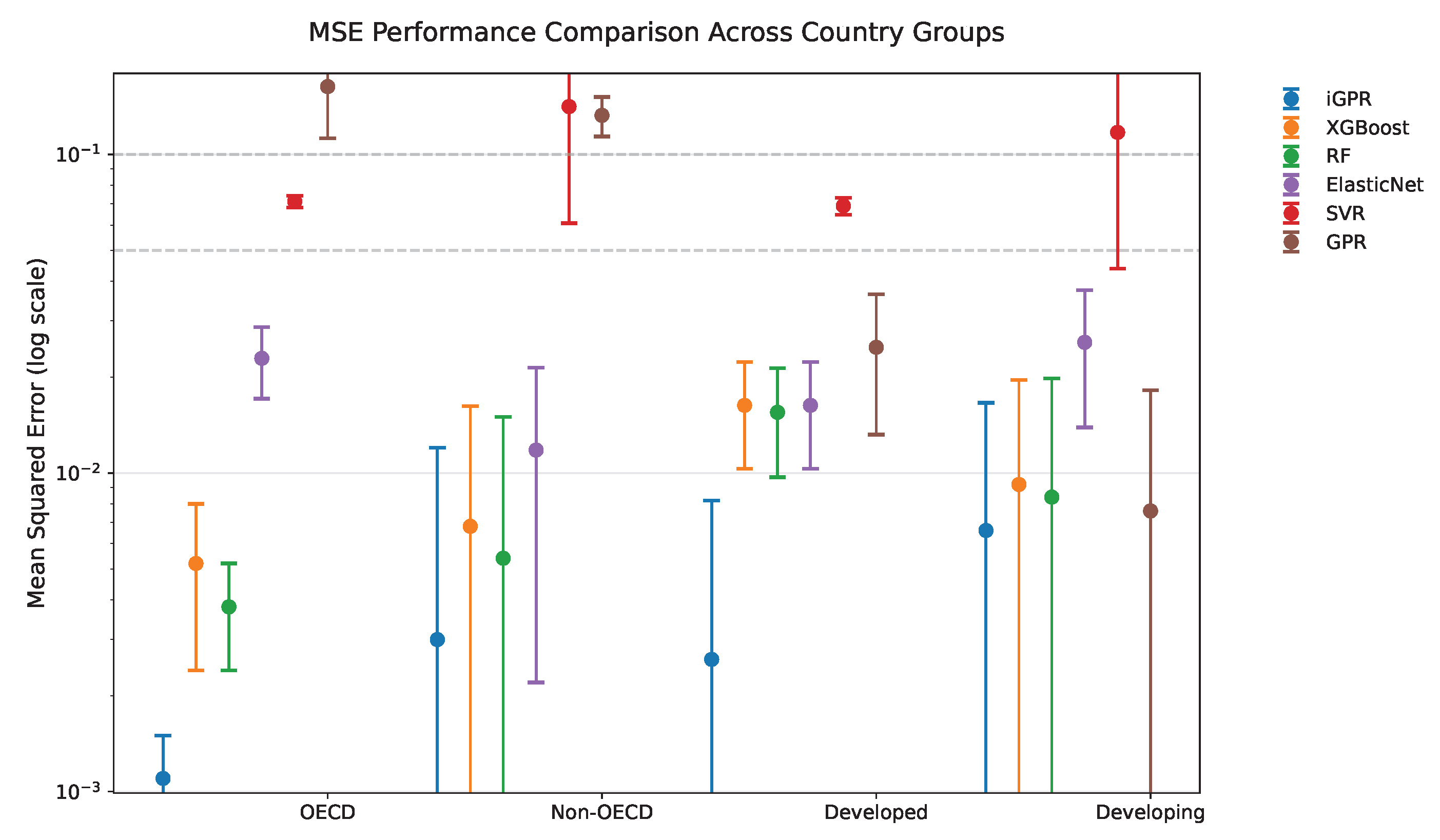
4.4. Country Heterogeneity Analysis

Table 6. MSE performance comparison across country categories.

Model	OECD		Non-OECD		Developed		Developing
	Mean	Std	Mean	Std	Mean	Std	Mean	Std
iGPR	0.0011	0.0002	0.0030	0.0045	0.0026	0.0028	0.0066	0.0050
XGBoost	0.0052	0.0014	0.0068	0.0047	0.0163	0.0030	0.0092	0.0052
RF	0.0038	0.0007	0.0054	0.0048	0.0155	0.0029	0.0084	0.0057
SVR	0.0711	0.0015	0.1412	0.0402	0.0689	0.0021	0.1172	0.0367
ElasticNet	0.0229	0.0029	0.0118	0.0048	0.0163	0.0030	0.0257	0.0059
GPR	0.1632	0.0255	0.1325	0.0094	0.0248	0.0058	0.0076	0.0053

shows the results. The IGPR algorithm we designed was run 10 times, yielding an MSE mean of 0.0011 for OECD countries and 0.0030 for non-OECD countries. This may indicate that the data from OECD countries has a higher degree of standardization, with less volatility in indicators, whereas non-OECD countries exhibit greater diversity in economic structures, and their data may contain more noise, leading to a higher MSE.

The IGPR algorithm outperformed other models in both country groups, but its relative advantage was more pronounced in non-OECD countries. In OECD countries, the performance gap narrowed compared to XGBoost (0.0048) and random forest (0.0035). This could be because the linear or more regularized features of OECD countries are better suited for tree-based models, while IGPR’s superior nonlinear modeling capabilities stand out in non-OECD countries.

The standard deviation of the IGPR algorithm over 10 runs in OECD countries was only 0.0007, an extremely low value indicating highly stable prediction results. This likely stems from standardized data collection and consistent economic policies. In contrast, the higher standard deviation observed in non-OECD countries reflects greater heterogeneity among these nations, yet it remains within a reasonable range, demonstrating the model’s robustness against noise.

The iGPR algorithm demonstrates strong predictive performance across both developed and developing countries, with a mean MSE of 0.0026 and 0.0066, respectively, significantly outperforming competing methods in most cases. This performance gap suggests that data from developed economies tends to be more standardized and less volatile, allowing iGPR to achieve exceptional accuracy (nearly 10× better than the next best model, GPR). In developing countries, while GPR comes closer in performance (MSE 0.0076 vs. iGPR’s 0.0066), iGPR maintains a clear advantage over other models, particularly in handling noisier, more heterogeneous data—as evidenced by its superior performance compared to SVR and ElasticNet. The algorithm also shows remarkable stability, with particularly low standard deviation (0.0028) in developed countries, reflecting consistent predictions in stable economic environments. Even in more volatile developing economies, where the standard deviation rises to 0.0050, iGPR remains more stable than alternative approaches. These results highlight iGPR’s dual strengths: outstanding precision in well-structured developed economies and robust adaptability in more complex developing contexts, making it a versatile and reliable choice for cross-national economic modeling. The particularly pronounced performance advantage in developed countries suggests that iGPR is especially effective at extracting patterns from high-quality, standardized data, while its maintained leadership in developing countries demonstrates impressive resilience to noise and variability.

Figure 3 presents the forest plot of the mean and standard deviation of different algorithms in OECD countries, non-OECD countries, developed countries, and developing countries under a linear scale. It can be clearly seen that the mean of the iGPR algorithm is lower than that of the other algorithms, and the length of the line segment is relatively short. Figure 4 shows the forest plot of the mean and standard deviation of different algorithms under a logarithmic scale, and the same conclusion can be drawn.

5. Conclusions and Policy Implications

By integrating spatial dependencies and nonlinear feature interactions through a hierarchical hybrid architecture, iGPR significantly outperforms traditional machine learning models (such as XGBoost, RF, and GPR) in terms of prediction accuracy (MSE = 0.0047) and robustness. Empirical evidence confirms that digitalization enhances carbon efficiency through scale and structural effects (ATE = 0.00895), with this effect being more significant in OECD countries (MSE = 0.0011). Based on the findings, the positive Average Treatment Effect (ATE) suggests that the degree of modernization has a significant positive impact on carbon emission efficiency. This impact is likely due to the scale and structural effects associated with modernization, which demonstrably promote improvements in carbon emission efficiency. Comparing five algorithms—Extreme Gradient Boosting, random forest, support vector regression, Elastic Net Regularized Regression, and Gaussian process regression—we differentiated geographical factors from other relevant indicators. By constructing a Gaussian kernel matrix using latitude and longitude coordinates and solving for the kernel matrix coefficients via the quasi-Newton method, we applied the iGPR (intrinsic Gaussian Process Regression) method for Gaussian regression on the other indicators. The approach demonstrated the lowest mean and standard deviation of mean squared error (MSE) across ten experiments, leading us to conclude that the method yields smaller errors and higher stability compared to traditional methods and offers advantages for causal inference in other domains. Therefore, to enhance carbon emission efficiency, governments can promote high-quality economic development by optimizing industrial structures, strengthening innovation-driven approaches, and improving economic systems. They can also strengthen infrastructure through transportation, energy, and communication networks, and enhance public services through education modernization, healthcare modernization, and the establishment of robust social security systems. Utilizing these methods can effectively reduce carbon emissions by increasing modernization levels.

The findings highlight several important policy implications for enhancing carbon emission efficiency through digital transformation: governments and international organizations should prioritize investments in digital infrastructure, such as broadband networks, smart grids, and IoT platforms, to directly improve energy management and reduce emissions. Encouraging innovation through targeted R&D funding and incentives for startups focused on clean technologies and digital solutions can amplify both economic and environmental gains. Digitalization should be explicitly integrated into climate policies, including national determined contributions (NDCs) and carbon trading schemes, leveraging digital platforms to improve transparency and efficiency. Education and digital skills training are essential to maximize the benefits of digital technologies and support consumer adoption of energy-efficient devices and practices. Additionally, targeted policies and international cooperation are needed to address challenges in developing regions, including infrastructure reliability, digital divides, and regulatory frameworks, facilitating effective technology transfer. Integrating digital solutions into traditional industries—such as manufacturing, agriculture, and transportation—can simultaneously boost productivity and reduce emissions. Policymakers should also expand green finance mechanisms, utilizing digital fintech platforms to mobilize resources for sustainable investments. Furthermore, governments can lead by example through digitalization of public services, promoting smart city initiatives and online public services that enhance overall efficiency. Finally, ensuring coordinated policy design that aligns digital and environmental strategies, alongside managing short-term transition costs and supporting workforce retraining, is crucial to fully realizing digitalization’s potential as a transformative driver of sustainable development and low-carbon economic growth.

While th study provides novel insights into how digitalization impacts carbon emission efficiency using the intrinsic Gaussian Process Regression (iGPR) model, several limitations highlight opportunities for future research. The analysis relied on country-level data and an aggregate digitalization measure, so future studies could leverage more granular data (city-level, firm-level) and differentiate specific digitalization dimensions (e.g., ICT infrastructure, digital skills, e-governance) to enhance understanding. The computational complexity of the iGPR approach (O(n³)) suggests exploring scalable approximations such as sparse Gaussian processes or simpler spatial kernels to handle larger datasets. Additionally, although we addressed endogeneity using instrumental variables, alternative causal inference strategies like quasi-experimental designs (difference-in-differences with broadband rollouts) or panel structural equation modeling could further clarify causality. The model’s Gaussian assumptions and kernel choices may overlook complex or nonlinear relationships, suggesting exploration of flexible alternatives like Bayesian additive regression trees or spatio-temporal Gaussian processes. Furthermore, applying the iGPR framework to other environmental domains (biodiversity, air quality, water efficiency) would test its generalizability, while interpreting and visualizing spatial random effects could provide policy-relevant insights about unexplained regional variations. Overall, addressing these limitations will enrich understanding of digitalization’s role in sustainable development.

References

1. Yoro, K.O.; Daramola, M.O. CO2 emission sources, greenhouse gases, and the global warming effect. In Advances in Carbon Capture; Elsevier: Amsterdam, The Netherlands, 2020; pp. 3–28. [Google Scholar]
2. Min, J.; Yan, G.; Abed, A.M.; Elattar, S.; Khadimallah, M.A.; Jan, A.; Ali, H.E. The effect of carbon dioxide emissions on the building energy efficiency. Fuel 2022, 326, 124842. [Google Scholar] [CrossRef]
3. Yang, Z.; Gao, W.; Han, Q.; Qi, L.; Cui, Y.; Chen, Y. Digitalization and carbon emissions: How does digital city construction affect China’s carbon emission reduction? Sustain. Cities Soc. 2022, 87, 104201. [Google Scholar] [CrossRef]
4. Sun, T.; Di, K.; Shi, Q. Digital economy and carbon emission: The coupling effects of the economy in Qinghai region of China. Heliyon 2024, 10, e26451. [Google Scholar] [CrossRef] [PubMed]
5. Wang, Q.; Zhang, Q. Foreign direct investment and carbon emission efficiency: The role of direct and indirect channels. Sustainability 2022, 14, 13484. [Google Scholar] [CrossRef]
6. Zhao, X.; Long, L.; Yin, S.; Zhou, Y. How technological innovation influences carbon emission efficiency for sustainable development? Evidence from China. Resour. Environ. Sustain. 2023, 14, 100135. [Google Scholar] [CrossRef]
7. Zhang, C.; Lin, J. An empirical study of environmental regulation on carbon emission efficiency in China. Energy Sci. Eng. 2022, 10, 4756–4767. [Google Scholar] [CrossRef]
8. Yu, Z.; Liu, Y.; Yan, T.; Zhang, M. Carbon emission efficiency in the age of digital economy: New insights on green technology progress and industrial structure distortion. Bus. Strategy Environ. 2024, 33, 4039–4057. [Google Scholar] [CrossRef]
9. Wang, Q.; Zhang, C.; Li, R. Towards carbon neutrality by improving carbon efficiency-a system-GMM dynamic panel analysis for 131 countries’ carbon efficiency. Energy 2022, 258, 124880. [Google Scholar] [CrossRef]
10. Jiang, H.; Hu, W.; Guo, Z.; Hou, Y.; Chen, T. E-commerce development and carbon emission efficiency: Evidence from 240 cities in China. Econ. Anal. Policy 2024, 82, 586–603. [Google Scholar] [CrossRef]
11. Liu, L.; Li, M.; Gong, X.; Jiang, P.; Jin, R.; Zhang, Y. Influence mechanism of different environmental regulations on carbon emission efficiency. Int. J. Environ. Res. Public Health 2022, 19, 13385. [Google Scholar] [CrossRef] [PubMed]
12. Fan, B.; Li, M. The effect of heterogeneous environmental regulations on carbon emission efficiency of the grain production industry: Evidence from China’s inter-provincial panel data. Sustainability 2022, 14, 14492. [Google Scholar] [CrossRef]
13. Jiang, P.; Li, M.; Zhao, Y.; Gong, X.; Jin, R.; Zhang, Y.; Li, X.; Liu, L. Does environmental regulation improve carbon emission efficiency? Inspection of panel data from inter-provincial provinces in China. Sustainability 2022, 14, 10448. [Google Scholar] [CrossRef]
14. Yao, S.; Su, X. Research on the nonlinear impact of environmental regulation on the efficiency of China’s regional green economy: Insights from the PSTR model. Discret. Dyn. Nat. Soc. 2021, 2021, 5914334. [Google Scholar] [CrossRef]
15. Wang, Q.; Zhang, C.; Li, R. Does environmental regulation improve marine carbon efficiency? The role of marine industrial structure. Mar. Pollut. Bull. 2023, 188, 114669. [Google Scholar] [CrossRef] [PubMed]
16. Xie, Z.; Wu, R.; Wang, S. How technological progress affects the carbon emission efficiency? Evidence from national panel quantile regression. J. Clean. Prod. 2021, 307, 127133. [Google Scholar] [CrossRef]
17. Zhang, S.; Xue, Y.; Jin, S.; Chen, Z.; Cheng, S.; Wang, W. Does Urban Polycentric Structure Improve Carbon Emission Efficiency? A Spatial Panel Data Analysis of 279 Cities in China from 2012 to 2020. ISPRS Int. J.-Geo-Inf. 2024, 13, 462. [Google Scholar] [CrossRef]
18. Zhang, Y.; Chen, M.; Zhong, S.; Liu, M. Fintech’s role in carbon emission efficiency: Dynamic spatial analysis. Sci. Rep. 2024, 14, 23941. [Google Scholar] [CrossRef] [PubMed]
19. Wu, Z.; Xu, X.; He, M. The Impact of Green Finance on Urban Carbon Emission Efficiency: Threshold Effects Based on the Stages of the Digital Economy in China. Sustainability 2025, 17, 854. [Google Scholar] [CrossRef]
20. Zhang, Y.; Hong, W. A significance of smart city pilot policies in China for enhancing carbon emission efficiency in construction. Environ. Sci. Pollut. Res. 2024, 31, 38153–38179. [Google Scholar] [CrossRef] [PubMed]
21. Pang, G.; Li, L.; Guo, D. Does the integration of the digital economy and the real economy enhance urban green emission reduction efficiency? Evidence from China. Sustain. Cities Soc. 2025, 122, 106269. [Google Scholar] [CrossRef]
22. Haefner, L.; Sternberg, R. Spatial implications of digitization: State of the field and research agenda. Geogr. Compass 2020, 14, e12544. [Google Scholar] [CrossRef]
23. Nan, S.; Huo, Y.; You, W.; Guo, Y. Globalization spatial spillover effects and carbon emissions: What is the role of economic complexity? Energy Econ. 2022, 112, 106184. [Google Scholar] [CrossRef]
24. Ritchie, H.; Roser, M. CO2 Emissions. Our World Data. 2020. Available online: https://ourworldindata.org/co2-emissions (accessed on 20 May 2025).
25. Aigner, D.; Lovell, C.K.; Schmidt, P. Formulation and estimation of stochastic frontier production function models. J. Econom. 1977, 6, 21–37. [Google Scholar] [CrossRef]
26. Tone, K. A slacks-based measure of efficiency in data envelopment analysis. Eur. J. Oper. Res. 2001, 130, 498–509. [Google Scholar] [CrossRef]
27. Wu, D.; Mei, X.; Zhou, H. Measurement and Analysis of Carbon Emission Efficiency in the Three Urban Agglomerations of China. Sustainability 2024, 16, 9050. [Google Scholar] [CrossRef]
28. Jiang, H.; Yin, J.; Qiu, Y.; Zhang, B.; Ding, Y.; Xia, R. Industrial carbon emission efficiency of cities in the pearl river basin: Spatiotemporal dynamics and driving forces. Land 2022, 11, 1129. [Google Scholar] [CrossRef]
29. Liu, Q.; Hao, J. Regional differences and influencing factors of carbon emission efficiency in the Yangtze River economic belt. Sustainability 2022, 14, 4814. [Google Scholar] [CrossRef]
30. Wang, H.; Liu, W.; Liang, Y. Measurement of CO2 Emissions Efficiency and Analysis of Influencing Factors of the Logistics Industry in Nine Coastal Provinces of China. Sustainability 2023, 15, 14423. [Google Scholar] [CrossRef]
31. Jiang, X.; Ma, J.; Zhu, H.; Guo, X.; Huang, Z. Evaluating the carbon emissions efficiency of the logistics industry based on a Super-SBM Model and the Malmquist Index from a strong transportation strategy perspective in China. Int. J. Environ. Res. Public Health 2020, 17, 8459. [Google Scholar] [CrossRef] [PubMed]
32. Gu, R.; Duo, L.; Guo, X.; Zou, Z.; Zhao, D. Spatiotemporal heterogeneity between agricultural carbon emission efficiency and food security in Henan, China. Environ. Sci. Pollut. Res. 2023, 30, 49470–49486. [Google Scholar] [CrossRef] [PubMed]
33. Li, J.; Li, S.; Liu, Q.; Ding, J. Agricultural carbon emission efficiency evaluation and influencing factors in Zhejiang province, China. Front. Environ. Sci. 2022, 10, 1005251. [Google Scholar] [CrossRef]
34. Liang, Z.; Chiu, Y.h.; Guo, Q.; Liang, Z. Low-carbon logistics efficiency: Analysis on the statistical data of the logistics industry of 13 cities in Jiangsu Province, China. Res. Transp. Bus. Manag. 2022, 43, 100740. [Google Scholar] [CrossRef]
35. Song, C.; Liu, Q.; Song, J.; Ma, W. Impact path of digital economy on carbon emission efficiency: Mediating effect based on technological innovation. J. Environ. Manag. 2024, 358, 120940. [Google Scholar] [CrossRef] [PubMed]
36. Wu, G.; Liu, X.; Cai, Y. The impact of green finance on carbon emission efficiency. Heliyon 2024, 10, e23803. [Google Scholar] [CrossRef] [PubMed]
37. Huang, Z.; Zhao, T.; Lai, R.; Tian, Y.; Yang, F. A comprehensive implementation of the log, Box-Cox and log-sinh transformations for skewed and censored precipitation data. J. Hydrol. 2023, 620, 129347. [Google Scholar] [CrossRef]
38. van Buuren, S.; Groothuis-Oudshoorn, K. mice: Multivariate Imputation by Chained Equations in R. J. Stat. Softw. 2011, 45, 1–67. [Google Scholar] [CrossRef]
39. Wang, Y.; Li, Y.; Li, H.; Dang, W.; Zheng, A. Study on the correlation between soil resistivity and multiple influencing factors using the entropy weight method and genetic algorithm. Electr. Power Syst. Res. 2025, 246, 111692. [Google Scholar] [CrossRef]
40. Zhang, H.; Gan, J. A reproducing kernel-based spatial model in Poisson regressions. Int. J. Biostat. 2012, 8, 28. [Google Scholar] [CrossRef] [PubMed]
41. Javed, H.; El-Sappagh, S.; Abuhmed, T. Robustness in deep learning models for medical diagnostics: Security and adversarial challenges towards robust AI applications. Artif. Intell. Rev. 2024, 58, 12. [Google Scholar] [CrossRef]
42. Tang, Y.; Wang, X.; Zhu, J.; Lin, H.; Tang, Y.; Tong, T. Robust Inference for Censored Quantile Regression. J. Syst. Sci. Complex. 2024, 38, 1730–1746. [Google Scholar] [CrossRef]
43. Farzana, A.; Samsudin, S.; Hasan, J. Drivers of economic growth: A dynamic short panel data analysis using system GMM. Discov. Sustain. 2024, 5, 393. [Google Scholar] [CrossRef]
44. Hansen, L.P. Large Sample Properties of Generalized Method of Moments Estimators. Econometrica 1982, 50, 1029–1054. [Google Scholar] [CrossRef]
Figure 1. Heatmap for the correlation between different variables.
Sustainability 17 06551 g001
Figure 2. Distribution of prediction errors for the baseline iGPR model.
Sustainability 17 06551 g002
Figure 3. Linear-scale MSE forest plot comparing predictive models.
Sustainability 17 06551 g003
Figure 4. Log-scale MSE forest plot for enhanced model comparison.
Sustainability 17 06551 g004