A Sustainable Approach to Modeling Human-Centric and Energy-Efficient Vehicle Acceleration Profiles in Non-Car-Following Scenarios

Abstract

Previous studies have described vehicle acceleration profiles in non-car-following scenarios; however, the underlying mechanisms governing these profiles remain incompletely understood. This study aims to enhance the understanding of these mechanisms by proposing an improved model based on an optimal control problem with two bounded conditions (OCP2B), segmenting vehicle acceleration curves into three distinct phases. Specifically, the proposed model imposes constraints on acceleration through maximum jerk and maximum acceleration functions, thereby capturing essential dynamics previously unexplained by conventional models. Our key contributions include establishing a comprehensive analytical framework for accurately describing vehicle acceleration profiles and elucidating critical characteristics overlooked in the prior literature. Our findings demonstrate that incorporating human-centric considerations, such as driving comfort, significantly enhances the model’s practical applicability. Moreover, the proposed approach provides crucial insights for designing autonomous vehicle (CAV) trajectories consistent with human driving behaviors and effectively predicts the movements of human-driven vehicles (HVs), thus facilitating smoother interactions and potentially reducing conflicts between CAVs and HVs.

1. Introduction

Driving/riding comfort and energy efficiency are key elements in achieving a sustainable transport system [1]. As Connected and Autonomous Vehicles (CAVs) become increasingly integrated into modern transportation, ensuring these qualities is essential for their widespread acceptance. In this context, understanding drivers’ behaviors is fundamental to improving user experience and fostering trust in CAVs [2]. This understanding is crucial for optimizing CAV performance by reducing user unfamiliarity and perceived risks. Studies [3,4,5,6] have shown that discomfort and perceived risk arise when the time headway between vehicles falls below a critical threshold or when a vehicle’s acceleration exceeds certain limits, as observed in driving experiments. Consequently, it is critical for CAVs to accommodate human driving habits by ensuring that vehicle acceleration remains within comfortable and safety ranges, thus promoting user comfort and safety. Moreover, understanding driver behavior enables CAVs to interpret drivers’ intentions and predict the movements of human-driven vehicles (HVs). This capability allows CAVs to avoid overly cautious driving behaviors [7], thereby enhancing their integration within the traffic system.

Vehicle acceleration constitutes a significant aspect of driving behavior. Drivers employ pedal control to shape a comfortable acceleration curve [3,4] while efficiently reaching their travel destinations. Studies [3,4] conducted driving simulations on drivers, revealing a preference for minimizing both acceleration and jerk. Acceleration adjustment plays a crucial role in influencing traffic flow, particularly at bottlenecks and intersections. Certain literature highlights how bounded acceleration leads to capacity drop phenomena in lane-drop bottlenecks [8,9], and similarly, it affects traffic flow discharge rates at signalized intersections [10]. Given these dual effects of acceleration, drivers must navigate a trade-off between mobility and driving comfort when adjusting their speed.

Understanding vehicle acceleration behavior is, therefore, essential, not only for capturing human intentions but also for enhancing the decision-making processes of Connected and Autonomous Vehicles (CAVs). By analyzing human-driven vehicle (HV) trajectories through roadside units, Connected and Autonomous Vehicles (CAVs) can accurately forecast HV behavior during acceleration. This predictive ability enables CAVs to make safer and more efficient decisions, as shown in reference [7]. However, applying machine learning to this task has an inevitable challenge. Attributes like maximum jerk and acceleration within HV trajectories can vary due to factors such as road slope, trip purpose, and weather conditions. Short-term observations of HV trajectories provide insights into a vehicle’s immediate acceleration performance, but (i) relying on long-term historical data for model training may fail to capture the critical driving intentions within the specific timeframe necessary for AVs. On the other hand, (ii) using only short-term data risks overfitting. A plausible solution to this dilemma is to integrate the intrinsic dynamics of vehicle acceleration into predictive models [11].

To this end, this study presents an understanding of vehicle acceleration in a non-car-following state. We explore the non-car-following state for the following reasons:

(i).

In congested traffic flows, the efficiency and sustainability of the traffic system largely depend on the discharge rate at bottlenecks, such as intersections and merging areas. These rates are significantly affected by the acceleration curves of the leading vehicle in a fleet [9]. However, the movement of the leading vehicle is not always influenced by interactions with other vehicles.

(ii).

In non-congested traffic flows, a non-car-following acceleration process is pervasive. Vehicles exhibit this process during starting-up phases (originating from intersections) and abrupt accelerations (transitioning from speed limit areas). This behavior affects traffic efficiency and interactions between human-driven vehicles (HVs) and connected and autonomous vehicles (CAVs). For instance, when a CAV intends to change lanes, an HV accelerating behind the CAV in an adjacent lane affects these interactions.

To explore how drivers leverage acceleration control to balance both driving comfort and mobility in non-car-following acceleration scenarios, this study proposes an interpretative model that reproduces vehicle acceleration curves based on an optimal control-problem framework. Specifically, an optimal control problem with two bounded conditions (OCP2B) is formulated to describe key properties of vehicle acceleration. This problem is analytically solvable using bounded acceleration functions. The derived acceleration curves are systematically characterized, and their distinct features are compared with previously observed patterns. The proposed model and subsequent analyses not only provide valuable insights into predicting human-driven vehicle (HV) trajectories but also contribute to the refinement of control strategies for CAVs.

As an acceleration vehicle dynamics model, this study focuses on driving comfort and energy consumption efficiency, which benefits the sustainability of transportation. Specifically, the contributions are two-fold.

• It presents a framework to generate a vehicle’s longitudinal acceleration form. Considering two types of bounded acceleration curves, the final acceleration curves have three segments, which can reproduce complicated acceleration curves of vehicles from real-world data.
• It investigates the influences of some factors on the critical parameters of the acceleration curves, e.g., the acceleration task. In addition, this study takes energy consumption into the framework and compares the acceleration curves with and without considering energy consumption.

The rest of this paper is organized as follows. The literature review is presented in Section 2, and a framework for generating vehicle acceleration curves is proposed in Section 3. Section 4 introduces a framework for generating vehicle acceleration profiles and conducts a comparative evaluation between the proposed acceleration model and existing approaches. Section 5 provides further discussion, elaborating on implications and broader insights derived from the findings. Finally, the last section summarizes the key contributions and conclusions drawn from this study.

2. Literature Review

The related literature concerning the driver’s acceleration curve can be categorized into two distinct groups. The first category includes studies that focus on modeling acceleration profiles—i.e., the mathematical or data-driven representation of acceleration over time or velocity during various driving scenarios. The second category encompasses investigations into drivers’ acceleration characteristics and preferences, including behavioral tendencies, individual differences, and comfort-related aspects.

2.1. Existing Acceleration Profile Models

In traffic flow theory, scholars have made plenty of efforts to understand the mechanism of vehicle acceleration variation in the car-following process [12,13,14,15,16,17,18], which was called traffic dynamics in [19]. In these studies, they typically offer a simplified and abstract representation of vehicle driving, with the primary goal of capturing and reproducing traffic dynamics. A vehicle’s acceleration is generally adjusted to match its velocity with the available spacing in car-following scenarios, thereby ensuring the stability of the simulated traffic flow. However, in some acceleration processes when the vehicle’s velocity varies in a wide range, e.g., start-up process in the intersection, vehicles always accelerate with a similar form [20,21,22,23,24,25,26], which was called vehicle dynamics [19]. The vehicle dynamics model offers key advantages, including its capability to accurately predict vehicle behavior using readily accessible input parameters, as well as its flexibility in estimating acceleration rates for various types of vehicles [27], thus benefiting the design of the advanced driver assistance system (ADAS). Three common vehicle dynamic models (i.e., acceleration profile models) are used to describe the vehicle’s acceleration form, including the constant acceleration model, linear decreasing acceleration model, and polynomial acceleration model [20].

The first two acceleration models were developed to describe the boundedness of a vehicle’s acceleration [9,28]. The constant acceleration model assumes that the acceleration remains steady during the acceleration phase, offering simplicity and computational efficiency, particularly suitable for basic traffic simulations and scenarios with short duration acceleration phases, such as queue discharge at intersections [24]. The linear decreasing acceleration model addresses some limitations of the constant acceleration model by incorporating a gradually reducing acceleration, more closely mirroring real-world driving patterns. This model is widely employed in traffic flow simulations, particularly for urban intersection scenarios, as it effectively captures the acceleration behavior of vehicles as they approach desired speeds [29].

However, both models fail to accurately capture vehicular dynamics during acceleration, particularly the nonlinear characteristics of acceleration behavior. A polynomial acceleration model was developed to address this issue. In addition, two famous car-following models, i.e., the Gipps model [12] and the intelligence driver model (IDM) [30], can also reproduce the nonlinearity of the vehicle’s acceleration curves.

These acceleration models can describe the boundedness or nonlinearity of a vehicle’s dynamics. Moreover, the polynomial acceleration model can accurately reproduce a vehicle’s dynamics. However, they must explain how the acceleration curves form and why these models can describe the vehicle’s dynamics. In addition, the above acceleration models cannot reproduce many factors’ influences on acceleration curves. These factors include the slope of the road, the vehicle’s performance, the drivers’ heterogeneity, and the acceleration task. Consequently, there remains a substantial scope to develop more integrative and physically grounded acceleration models.

2.2. Drivers’ Preferences on Different Acceleration Styles

Much of the related literature investigated drivers’ preferences for different driving styles. Elander et al. [31] described driving style as a habitual pattern of driving behavior. This encompasses an individual’s preferred driving speed, personal criteria for overtaking, typical headway distance, and the degree to which they adhere to traffic regulations. The existing literature [32,33] emphasized the significance of acceleration behavior—an inherent reflection of individual preferences for speed changes—as a key factor in distinguishing different driving styles.

Some studies [3,4,34] investigated how automated vehicles should drive to ensure passenger comfort. Bellem et al. [3,4] conducted simulation experiments to identify comfortable driving strategies, focusing on key maneuvers such as lane changes, accelerations, and decelerations. Ksander N. et al. [34] sought to establish precise and interpretable metrics of perceived discomfort in response to acceleration pulses with varying characteristic profiles.

To ensure passenger comfort and reflect realistic driving behaviors, it is essential to develop an acceleration model that constrains both acceleration and jerk within acceptable limits. Müller et al. [32] conducted experiments to investigate the human perception of longitudinal acceleration based on the idea that vehicle acceleration is a physical stimulus for drivers. The results of this study indicate that the difference in acceleration is not noticeable for drivers when the difference is less than a threshold (0.1 ${\mathrm{m}/\mathrm{s}}^2$ for maximum acceleration). Bae et al. [35] proposed the Occupant’s Preference Metric (OPM) that defines a preferred lateral and longitudinal acceleration region with a maximum allowable jerk for users. In this study, the author indicated that the CAV’s acceleration and jerk values are reasonable to set the limit value around 2 ${\mathrm{m}/\mathrm{s}}^2$ and 0.9 ${\mathrm{m}/\mathrm{s}}^2$. The results of this study provide some insights into the present study for setting reasonable parameters of the acceleration model. Additionally, investigated optimal acceleration control strategies to enhance ride comfort while maintaining powertrain efficiency in hybrid electric vehicles. They demonstrated, through simulation-based optimization using genetic algorithms and validated via dynamic programming and sequential quadratic programming, that carefully optimized acceleration curves and power-split strategies significantly improved passenger comfort without compromising powertrain performance or energy demand. Additionally, Anselma [36] investigated optimal acceleration control strategies to enhance ride comfort while maintaining powertrain efficiency in hybrid electric vehicles. They demonstrated, through simulation-based optimization using genetic algorithms and validated via dynamic programming and sequential quadratic programming, that carefully optimized acceleration curves and power-split strategies significantly improved passenger comfort without compromising powertrain performance or energy demand.

Studies focusing on driver preferences emphasize that acceleration profiles inherently reflect personal driving habits, such as preferred speeds, overtaking criteria, and adherence to traffic regulations. Investigations into passenger comfort have underscored the necessity of constraining acceleration and jerk within perceptually acceptable thresholds. Experimental studies indicate specific human perceptual limits, recommending acceleration and jerk boundaries to optimize comfort. Moreover, optimized acceleration strategies have been demonstrated to significantly enhance passenger comfort while preserving energy efficiency, emphasizing the practical value of carefully calibrated acceleration models in advanced vehicle control systems.

2.3. Differences and Innovations of This Study Compared to Existing Research

Previous studies investigating vehicle acceleration have predominantly focused on simplified acceleration profiles, primarily within car-following scenarios or under highly constrained conditions. These conventional models, including constant, linear decreasing, and polynomial acceleration representations, typically emphasize computational simplicity or empirical fitting, often neglecting the detailed exploration of intrinsic vehicular dynamics and human behavioral factors. Consequently, existing acceleration models inadequately explain the underlying mechanisms driving observed acceleration behaviors, particularly in non-car-following situations.

This study significantly advances the existing body of research by introducing a novel interpretative framework, specifically addressing vehicle acceleration in non-car-following states through the formulation of an optimal control problem with two bounded conditions (OCP2B). Distinct from prior approaches, the OCP2B model systematically incorporates critical human-centric considerations, including constraints on maximum jerk and acceleration, thereby capturing essential dynamics previously overlooked in conventional representations. These enhancements enable more precise replication of realistic vehicle acceleration curves, as validated against real-world driving data.

A primary innovation of this work lies in segmenting acceleration profiles into three analytically distinct phases, facilitating a deeper understanding of acceleration dynamics and offering interpretability that transcends the scope of purely data-driven or simplistic models. Furthermore, this study uniquely integrates factors such as energy consumption into the acceleration modeling framework, providing insights into how efficiency considerations influence driver acceleration behaviors.

Additionally, by embedding intrinsic vehicular dynamics into predictive frameworks, this research circumvents potential overfitting issues associated with limited observational periods, thus offering robust predictions of human-driven vehicle behaviors crucial for enhancing interactions between connected and autonomous vehicles (CAVs) and human-driven vehicles (HVs).

Collectively, these methodological innovations and theoretical contributions distinctly position this study within the existing literature, highlighting its potential to substantially inform the development of sophisticated vehicle control strategies, improve traffic flow efficiency, and enhance user comfort and safety in intelligent transportation systems.

3. Methods

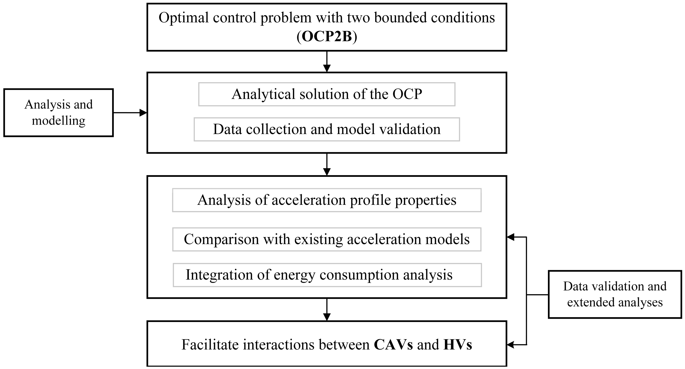
The overall research framework is structured around the development and application of OCP2B to model sustainable vehicle acceleration profiles in non-car-following scenarios. The research follows the steps outlined below in Figure 1. In order to verify the analytical solution, real-world acceleration trajectories are used to fit the model and provide insights from empirical patterns. Compared against existing acceleration models to assess its advantages, and analysis on energy consumption and CAV–HV interaction further demonstrates its value on sustainability.

3.1. The Formulation of the Optimal Control Problem

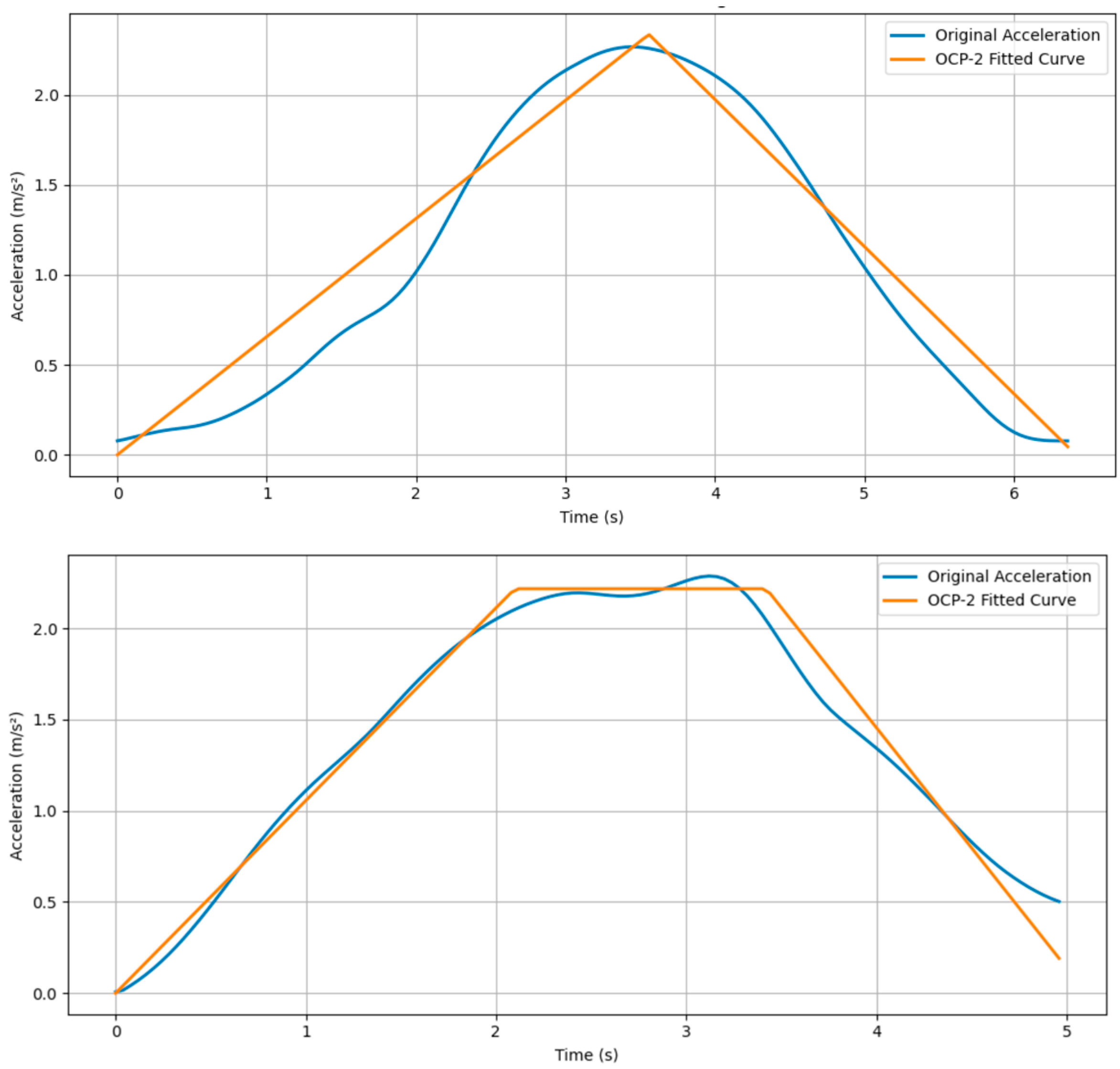
In this section, we show that a vehicle’s acceleration form can be derived from an optimal control problem considering the driver’s intention to move fast and drive comfortably. It is worth noting that the “zero-jerk” condition (due to the limited performance of the vehicle’s powertrain, the initial and final value of the vehicle’s jerk is zero in an acceleration process) is not considered in the optimal control problem because we cannot derive the analytical solution of the optimal control problem when the condition is considered, and it has few influences on the aggregate properties of the acceleration curves (it will be proven by the real-world data in Figure 1).

The acceleration task in a non-car-following state is studied in this study, i.e., we do not consider the interaction between vehicles (the reader can find the reasoning within Section 1). In the non-car-following state, drivers attempt to speed up and finish the acceleration task quickly. In addition, drivers desire a comfortable driving experience.

In such an acceleration task, the vehicle speeds up from the initial velocity $v_0$ to the final velocity $v_f$ in the time period $[t_0,t_f]$, and drivers attempt to finish a fixed driving distance $L$ with the least amount of time $(t_f-t_0)$. The travel time is formulated as

$$T_L={\displaystyle \frac{1}{v_f}}\left(L-{\displaystyle {\int }_{t_0}^{t_f}v}dt\right)+t_f$$

(1)

Thus, the driver’s travel time cost is formulated as

$$J_{\mathrm{t}}={\alpha }_{\mathrm{VOT}}\left[{\displaystyle \frac{1}{v_f}}\left(L-{\displaystyle {\int }_{t_0}^{t_f}v}dt\right)+t_f\right]$$

(2)

where ${\alpha }_{\mathrm{VOT}}$ is the parameter that represents the driver’s value of time.

No literature explicitly relates the vehicle’s dynamics and the driver’s discomfort during the acceleration process. However, researchers assumed that discomfort increases with the square of the vehicle’s acceleration. High-order terms of acceleration, e.g., $a^3$ and $a^{2}v$, can be expanded to $a^2, a$ and $av$ when $a$ is small. Therefore, we assume that the driving discomfort is formulated as

$$J_{\mathrm{d}}={\alpha }_{\mathrm{VOC}}\left[{\displaystyle {\int }_{t_0}^{t_f}\left({\theta }_{1}a+{\theta }_2{a}^2+{\theta }_{3}av\right)}dt\right]$$

(3)

where ${\alpha }_{\mathrm{VOC}}$ is the unit cost of driving discomfort, and ${\theta }_1, {\theta }_2, {\theta }_3$ are the parameters relevant to the driving discomfort. Note that jerk is also considered with its boundedness to represent the driving comfort in the following content.

Drivers control the acceleration pedal to finish the acceleration task and minimize the total cost $J=J_{\mathrm{t}}+J_{\mathrm{d}}-{\alpha }_{\mathrm{VOT}}\cdot {\displaystyle \frac{L}{v_f}}$. The formulation of $J$ can be simplified as follows:

$$J={\beta }_1{t}_f+{\displaystyle {\int }_{t_0}^{t_f}\left({\beta }_{2}v+{\beta }_{3}a+{\beta }_4{a}^2+{\beta }_{5}av\right)}dt$$

(4)

where

$$\left\{\begin{array}{l}{\beta }_1={\alpha }_{\mathrm{VOT}},\\ {\beta }_2=\hspace{0.33em}-{\displaystyle \frac{{\alpha }_{\mathrm{VOT}}}{v_f}},\\ {\beta }_3={\alpha }_{\mathrm{VOC}}{\theta }_1,\\ {\beta }_4={\alpha }_{\mathrm{VOC}}{\theta }_2,\\ {\beta }_5={\alpha }_{\mathrm{VOC}}{\theta }_3.\end{array}\right.$$

(5)

The driver’s cost in the acceleration process depends on three instantaneous variables, i.e., velocity, acceleration, and jerk. The purpose of this study is to propose a method to obtain an optimal acceleration form. It is an optimal control problem (OCP). For the leading vehicle, $x(t)={\left[a(t),v(t)\right]}^T$ is the longitudinal dynamics vector, and $\dot{x}(t)=f(x,u,t)={\left[j(t),a(t)\right]}^T$ is the state dynamic vector, where $u(t)=j(t)$ is the control input of the system, and $f(x,u,t)$ is the state equations. The OCP is formulated as

$${\min }_j{\beta }_1{t}_f+{\displaystyle {\int }_{t_0}^{t_f}\left({\beta }_{2}v+{\beta }_{3}a+{\beta }_4{a}^2+{\beta }_{5}av\right)} \text{(OCP)}$$

$$\mathrm{s}.\mathrm{t}.\hspace{1em}\left\{\begin{array}{l}|j(t)|\hspace{0.33em}\hspace{0.33em}\le \hspace{0.33em}\hspace{0.33em}{j}_{\max },\\ a(t_0)\hspace{0.33em}\hspace{0.33em}=\hspace{0.33em}\hspace{0.33em}a(t_f)\hspace{0.33em}\hspace{0.33em}=\hspace{0.33em}\hspace{0.33em}0,\\ a(t)\hspace{0.33em}\hspace{0.33em}\le \hspace{0.33em}\hspace{0.33em}{a}_{\max }(v(t)),\\ v(t_0)\hspace{0.33em}\hspace{0.33em}=\hspace{0.33em}\hspace{0.33em}{v}_0,\\ v(t_f)\hspace{0.33em}\hspace{0.33em}=\hspace{0.33em}\hspace{0.33em}{v}_f.\end{array}\right.$$

(6)

$|j(t)|\hspace{0.33em}\hspace{0.33em}\le \hspace{0.33em}\hspace{0.33em}{j}_{\max }$ states that the jerk is bounded by $j_{\max }$ and $-j_{\max }$, which also represent the driving comfort that abrupt change of acceleration should be avoided [3,4]; $a(t_0)\hspace{0.33em}\hspace{0.33em}=\hspace{0.33em}\hspace{0.33em}a(t_f)\hspace{0.33em}\hspace{0.33em}=\hspace{0.33em}\hspace{0.33em}0$ is the “zero-acceleration” condition at the beginning and end of the acceleration process; $a(t)\hspace{0.33em}\hspace{0.33em}\le \hspace{0.33em}\hspace{0.33em}{a}_{\max }(v(t))$ indicates that vehicle’s acceleration is bounded caused by the performance of the vehicle [9] or driver’s expectation [4]; $v(t_0)\hspace{0.33em}\hspace{0.33em}=\hspace{0.33em}\hspace{0.33em}{v}_0$ and $v(t_f)\hspace{0.33em}\hspace{0.33em}=\hspace{0.33em}\hspace{0.33em}{v}_f$ indicates the acceleration task is that the vehicle should accelerate from $v_0$ to $v_f$.

The OCP can also be formulated as

$$\min J=\min \left(G\left[x\left(t_f\right),t_f\right]+{\displaystyle {\int }_{t_0}^{t_f}F\left[x\left(t\right),u\left(t\right),t\right]dt}\right)$$

(7)

where $G\left[x\left(t_f\right),t_f\right]$ is the Mayer term of the cost function; $F\left[x\left(t\right),u\left(t\right),t\right]$ is the Lagrange term of the cost function, i.e., ${\beta }_{2}v+{\beta }_{3}a+{\beta }_4{a}^2+{\beta }_{5}av$.

3.2. The Solutions of the OCP

The Hamiltonian function of the above optimal problem is

$$\mathcal{H}=F\left(x,u,t\right)+{\lambda }^{T}f\left(x,u,t\right)$$

(8)

where $\lambda =[{\lambda }_1,{\lambda }_2]$ is the vector of the co-state variable that satisfies the following condition when $x$ reaches the optimal value.

$$\stackrel{.}{\lambda }=-{\displaystyle \frac{\partial \mathcal{H}}{\partial x}}$$

(9)

It is evident that $\dot{x}$ and $\dot{\lambda }$ can be solved with the bounded conditions of Equation (6). We do not need to add any additional conditions to constrain the co-state variables.

Regarding the solution of the OCP, the control variable $j$ must satisfy Pontryagin’s maximum principle (PMP), i.e.,

$$\mathcal{H}(x^{*},u^{*},{\lambda }^{*},t)\le \mathcal{H}(x^{*},u,{\lambda }^{*},t)\hspace{0.33em}\hspace{0.33em}\hspace{1em}t\in [t_0,t_f]$$

(10)

where the PMP can be alternatively formulated as the following necessary condition ${\displaystyle \frac{\partial H}{\partial u}}=0$. For the specific OCP, $H_u={\lambda }_2$, i.e., the Hamiltonian is an affine function of the control input $j$. This means that the optimal control should switch between $j_{\max }$ and $-j_{\max }$, which is determined by the sign of ${\lambda }_2$. There is an exception to this rule when $H_u=0$, and the optimal control will be $j_s$ under this condition (the necessary condition (that the optimal control is equal to $j_s$) is that $\left|j_s\right|>j_{\max }$.). In other words, the optimal control can be formulated as follows:

$$j^{*}=\left\{\begin{array}{cc}{j}_{\max }& \mathrm{if}\hspace{0.33em}\hspace{0.33em}{\lambda }_2<0\\ j_s& \mathrm{if}\hspace{0.33em}\hspace{0.33em}{\lambda }_2=0\\ -j_{\max }& \mathrm{if}\hspace{0.33em}\hspace{0.33em}{\lambda }_2>0\end{array}\right.$$

(11)

This control is known as the “bang-singular-bang” control, whose optimal solution may form a singular arc (the optimal solution is $j_s$, which is not the bound of the jerk) when ${\lambda }_2=0$. The necessary condition that the singular arc exists is that the time derivatives of $H_u$ must vanish [37], i.e.,

$${\displaystyle \frac{d^n}{d{t}^n}}\left({\displaystyle \frac{\partial \mathcal{H}}{\partial u}}\right)=0$$

(12)

Rewriting the co-state in Equation (9),

$$\left\{\begin{array}{l}{\dot{\lambda }}_1=-{\beta }_2-{\beta }_5\alpha \\ {\dot{\lambda }}_2=-({\beta }_3+2{\beta }_{4}a+{\beta }_{5}v+{\lambda }_1)\end{array}\right.$$

(13)

Substituting Equation (13) into Equation (12), it is evident that $j_s={\displaystyle \frac{{\beta }_2}{2{\beta }_4}}$. The jerk $j$ will select its value from the set $\mathcal{J}=\left\{j_{\max },-j_{\max },j_s,{\dot{a}}_{\max }(v)\right\}$.

3.3. The Lower-Order Optimal Control Problem

In this subsection, the lower-order version of the specific OCP is formulated as the following optimal problemin which the optimal control variable is acceleration.

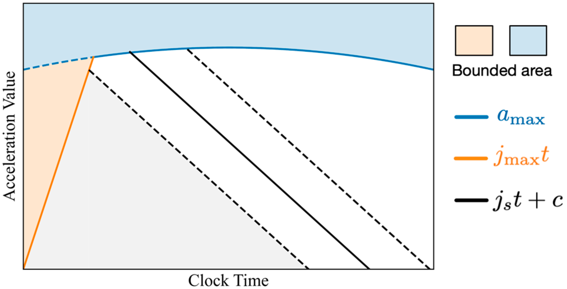
The vehicle’s acceleration is bounded by $a(t)\hspace{0.33em}\hspace{0.33em}\le \hspace{0.33em}\hspace{0.33em}{j}_{\max }t$ and $a(t)\hspace{0.33em}\hspace{0.33em}\le \hspace{0.33em}\hspace{0.33em}{a}_{\max }(v(t))$ in Equation (14), as shown in Figure 2.

$${\min }_a{\beta }_1{t}_f+{\displaystyle {\int }_{t_0}^{t_f}\left({\beta }_{2}v+{\beta }_{3}a+{\beta }_4{a}^2+{\beta }_{5}av\right) \text{(OCP-2)}}$$

$$\mathrm{s}.\mathrm{t}.\hspace{1em}\left\{\begin{array}{l}a(t)\hspace{0.33em}\hspace{0.33em}\le \hspace{0.33em}\hspace{0.33em}{j}_{\max }t,\\ a(t_0)\hspace{0.33em}\hspace{0.33em}=\hspace{0.33em}\hspace{0.33em}a(t_f)\hspace{0.33em}\hspace{0.33em}=\hspace{0.33em}\hspace{0.33em}0,\\ a(t)\hspace{0.33em}\hspace{0.33em}\le \hspace{0.33em}\hspace{0.33em}{a}_{\max }(v(t)),\\ v(t_0)\hspace{0.33em}\hspace{0.33em}=\hspace{0.33em}\hspace{0.33em}{v}_0,\\ v(t_f)\hspace{0.33em}\hspace{0.33em}=\hspace{0.33em}\hspace{0.33em}{v}_f.\end{array}\right.$$

(14)

The solution of OCP-2 is formulated as

$$a(t)=\min \left\{j_{\max }t,a_{\max }(v(t)),{\displaystyle \frac{-{\beta }_3+{\beta }_{5}v+{\lambda }_a}{2{\beta }_4}}\right\}$$

(15)

where ${\lambda }_a$ is the co-state variable in OCP-2. It is evident that

$${\displaystyle \frac{d}{dt}}\left({\displaystyle \frac{-{\beta }_3+{\beta }_{5}v+{\lambda }_a}{2{\beta }_4}}\right)={\displaystyle \frac{{\beta }_2}{2{\beta }_4}}=j_s$$

(16)

The solution of OCP-2 satisfies the constraints of OCP, which is illustrated by Figure 1. For a specific vehicle (driver), $a_{\max }$ and $j_{\max }$ are fixed, but the black line ($c+j_{s}t$) is not fixed. It should translate along the blue and orange solid line to make the equation ${\displaystyle {\int }_{t_0}^{tf}a}(t)dt=v_f-v_0$ (the area of grey zone in Figure 1) hold. Thus, the solution of OCP can be represented as

$$j_{\max }\to ({\dot{a}}_{\max })\to j_s(-j_{\max })$$

(17)

Equation (15) indicates that the slope of the vehicle’s acceleration should switch from $j_{\max }$ to the derivative of $a_{\max }$ if the maximum value of the acceleration can reach the curve of $a_{\max }$, and then switch to $j_s$ or $-j_{\max }$. Whether the final state is $j_s$ or $-j_{\max }$ depends on the size comparison of the absolute value of $j_s$ and $-j_{\max }$.

Thus, the acceleration curves should fall into the following categories in

Table 1. The categories of acceleration curves.

Type	Categories of Acceleration Curve
1	$j_{\max }\to j_s$
2	$j_{\max }\to -j_{\max }$
3	$j_{\max }\to {\dot{a}}_{\max }\to j_s$
4	$j_{\max }\to {\dot{a}}_{\max }\to -j_{\max }$

.

4. Results

We validate the theoretical framework using empirical vehicle trajectory data from the inD dataset [38]. Validation confirms that the OCP2B-derived piecewise linear functions accurately replicate essential characteristics of observed acceleration behaviors, demonstrating the model’s robustness and applicability. Derived acceleration profiles under two bounded acceleration conditions are systematically analyzed, categorized, and evaluated to identify parameters significantly influencing driver behavior and vehicle dynamics. Traditional acceleration models, such as constant, linear-decreasing, and polynomial forms, are critically assessed, revealing limitations in accurately representing realistic vehicle dynamics compared to the proposed framework. The model is subsequently extended by incorporating electric vehicle energy consumption. Inclusion of energy efficiency considerations substantially modifies acceleration profiles, notably affecting curvature in the terminal acceleration phase. This extension highlights how energy efficiency shapes driver acceleration behaviors, underscoring the model’s relevance to sustainable mobility and advanced trajectory planning.

4.1. Datasets Description and Processing

To validate the effectiveness of the proposed OCP2B framework, we conducted experiments using the inD dataset [38]. This dataset comprises over 11,500 trajectories, with each trajectory corresponding to a single road user—either a vehicle or a pedestrian—and recorded as a timestamped sequence. The road environments represented in the dataset include highways, straight urban roads, and intersections, offering diverse driving contexts. The recorded trajectories encompass various driving behaviors such as intersection crossings, turning maneuvers, and car-following scenarios. A summary of the dataset’s key characteristics is presented in

Table 2. Database used in this work.

Dataset	Locations	Nums of Tracks	Road User Types	Data Frequency	Maps
inD	Urban intersections (4)	11,500	Bicycle, car, truck, bus	25 Hz	yes

. In this study, we specifically selected independent vehicle acceleration events at intersections under non-car-following conditions—namely, scenarios where drivers’ acceleration behaviors were not directly influenced by preceding vehicles—in order to explicitly characterize vehicle acceleration dynamics in non-car-following states. Vehicle acceleration data were extracted accordingly. Subsequently, we employed a piecewise trajectory fitting method based on the classification criteria outlined in Table 1, utilizing the least squares approach.

During the preprocessing stage of the inD dataset, we first represented each trajectory as a four-tuple <id, timestamp, type, path>, where id and timestamp denote the unique identifier and initial timestamp of each trajectory, respectively. The type explicitly specifies the category of road users included in this study—namely, bicycles, cars, and buses. The path comprises a sequence of waypoints, with each waypoint characterized by a triplet <pos, acc, direc>, where pos indicates the central position coordinates of the vehicle, acc represents the instantaneous acceleration, and direc denotes the vehicle’s heading direction at each waypoint. Specifically, our data processing involved three steps: first, we identified trajectories representing non-car-following scenarios, i.e., independent acceleration events in which drivers’ acceleration behaviors were not directly influenced by preceding vehicles. Second, we extracted instantaneous acceleration data from these selected trajectories. Finally, we applied a piecewise regression approach to precisely segment and fit the acceleration curves.

The specific methodological steps are detailed as follows:

(1)

Based on the optimal control theoretical framework and considering the dual constraints of acceleration and jerk, the acceleration process is explicitly divided into distinct segments.

(2)

Initial candidate breakpoints are identified, followed by iterative optimization based on minimizing the overall residual sum of squares. A grid-search strategy is applied iteratively to ensure each segment’s statistical and theoretical validity.

(3)

Once breakpoints are finalized, linear regression is separately applied to each segment. The acceleration within segment $i$ is modeled as follows:

$$a(t)={\alpha }_i+{\beta }_{i}t+{\epsilon }_i\mathrm{t}\in \left[t_i,t_{i+1}\right]$$

where ${\alpha }_i$ and ${\beta }_i$ are fitting parameters; ${\epsilon }_i$ is the residual term; and $\left[t_i,t_{i+1}\right]$ is the time interval of the segment.

4.2. Verification of the Formulation and Observation from Data

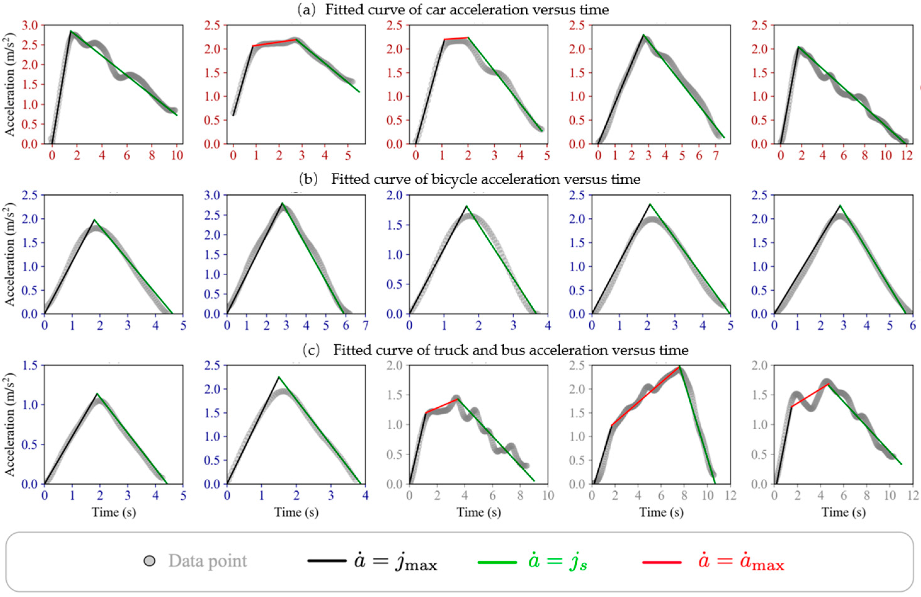
The preceding subsection developed a mathematical framework for deriving vehicular acceleration profiles in non-car-following scenarios. Drivers dynamically balance mobility requirements against comfort constraints when executing acceleration maneuvers. We present a fitting curve of acceleration curves (w.r.t. time) with the inD dataset [38], as shown in Figure 3. Raw data from the inD dataset provided instantaneous velocity and positional information at high temporal resolution. Acceleration profiles were derived by numerically differentiating the velocity data. We extract the acceleration data of individuals and use the least squares method to obtain the piecewise trajectory with the rules in Table 1.

The temporal evolution of vehicle acceleration can be accurately represented by piecewise linear functions, thereby validating the proposed framework’s effectiveness.

From Figure 3, some characteristics of the data are concluded as follows:

(1)

The acceleration value always increases from 0 to its bounded value [ $a_{\max }(v)$ ] quickly with a constant slope.

(2)

The bounded acceleration value always increases with velocity (see Figure 3).

(3)

Drivers can hardly decrease the value of acceleration smoothly, except for cyclists.

Remark 1.

Due to the constraint of the vehicle’s powertrain system, the vehicle’s jerk ($\mathit{j}={\displaystyle \frac{\mathit{d}\mathit{a}}{\mathit{d}\mathit{t}}}$) is continuous. In addition, $\mathit{j}\mathit{(}{\mathit{t}}_{\mathit{0}}\mathit{)}=\mathit{j}\mathit{(}{\mathit{t}}_{\mathit{f}}\mathit{)}=0$ (“zero-jerk” conditions). Thus, the acceleration curve is convex in its beginning and ending segments. The joints of the adjacent segments of the acceleration curve are concave. The “zero-jerk” condition should be considered when applying the results in this study by smoothing the acceleration curves deduced with the OCP.

The properties of acceleration curves in Remark 1 are irrelevant to the driver’s choice and manipulation, and they have little effect on the overall performance of the vehicle’s acceleration. In trajectory planning applications, acceleration profiles can be smoothed at segments containing non-differentiable points to ensure kinematic feasibility. From Figure 3, the properties of and the differences between the acceleration curves of the three types of vehicles are presented as follows.

4.3. Constant Bounded Acceleration

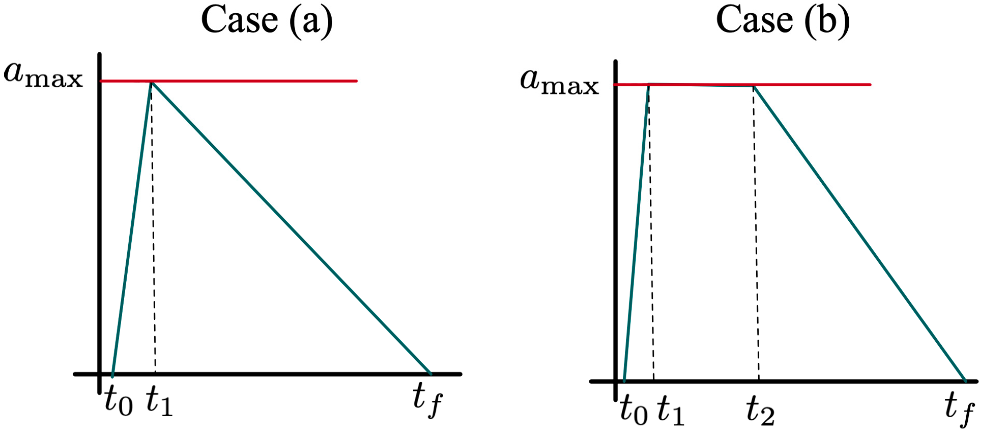
When a vehicle’s acceleration is bounded by a constant value, $a_{\max }$.

A vehicle’s acceleration curve in one acceleration task can be classified into two cases, as shown in Figure 4. For the first case in Figure 4a, there is only one point in the acceleration curve whose value is $a_{\max }$ at most. For the other case, the vehicle keeps speeding up with $a_{\max }$ in a time period.

Proposition 1.

The switch condition from case (a) to case (b) is ${\mathit{v}}_{\mathit{f}}-{\mathit{v}}_{\mathit{0}}>-{\displaystyle \frac{1}{2}}{\displaystyle \frac{{\mathit{j}}_{\max }-{\mathit{j}}_s}{{\mathit{j}}_s{\mathit{j}}_{\max }}}{\mathit{a}}_{\max }^2$.

Proof. 

In case (a), the constant bounded acceleration curve is not active. Thus, the area within the diagram in Figure 4a is less than ${\displaystyle \frac{1}{2}}{\displaystyle \frac{a_{\max }^2(j_{\max }+j_s)}{j_{\max }{j}_s}}$, i.e.,

$$v_f-v_0\le -{\displaystyle \frac{1}{2}}{\displaystyle \frac{a_{\max }^2(j_{\max }-j_s)}{j_{\max }{j}_s}}$$

(18)

For a specific vehicle/driver, $j_s$ and $j_{\max }$ is always fixed in one trip; thus, the RHS of Equation (18) is fixed. The acceleration curve is a triangle when the acceleration task ($v_f-v_0$) is less than the RHS. Otherwise, the acceleration curve is trapezoid. The constant bounded acceleration ($a_{\max }$) varies with drivers other than vehicles. The result in Proposition 1 can be reformulated as,

$${\displaystyle \frac{{\beta }_2}{{\beta }_4}}<{\displaystyle \frac{j_{\max }{a}_{\max }^2}{a_{\max }^2-2(v_f-v_0)j_{\max }^2}}$$

(19)

The results of Proposition 1 can be used to design the trajectories of CAVs in acceleration processes and help CAVs to predict the motions of the surrounding vehicles. □

Remark 2.

The formulations of critical variables for the acceleration curves with constant bounded acceleration can be easily derived with Figure 3 and the solutions of OCP; thus, the derivations are omitted here.

4.4. Linear-Increasing Bounded Acceleration

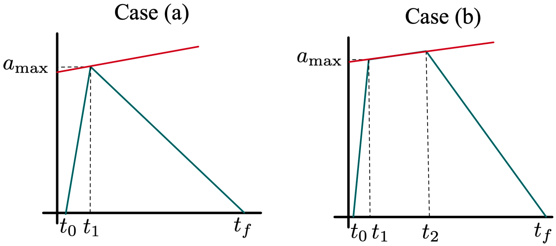
When a linear-increasing acceleration curve bounds a vehicle’s acceleration, the acceleration curves can also be classified into two cases, as shown in Figure 5.

For the two cases in Figure 5, the switch condition from case (a) to case (b) is also presented in Proposition 1. If the bounded acceleration is a function of time, i.e., $a_{\mathrm{b}}=a_{\mathrm{b}}(t)=c_{1}t+c_2$, the formulations of some critical variables are listed as follows.

$$\left\{\begin{array}{l}{t}_1=\min \left\{{\displaystyle \frac{c_2}{j_{\max }-c_1}},\sqrt{{\displaystyle \frac{2j_s(v_f-v_0)}{(j_s-j_{\max })j_{\max }}}}\right\},\\ t_2=t_1+\max \{0,\delta \},\\ t_f=\min \left\{{\displaystyle \frac{c_2}{j_{\max }-c_1}},\sqrt{{\displaystyle \frac{2(j_s-j_{\max })(v_f-v_0)}{j_s{j}_{\max }}}}\right\}.\end{array}\right.$$

(20)

where the formulation of $\delta$ is derived and presented in Appendix A. With these formulations of $t_1,t_2$ and $t_f$, AV can easily construct a trajectory that is suitable for humans (or human driving habits). Also, AVs can easily predict some trajectories of HVs that may have conflicts with AVs.

4.5. Three Existing Acceleration Profile Models

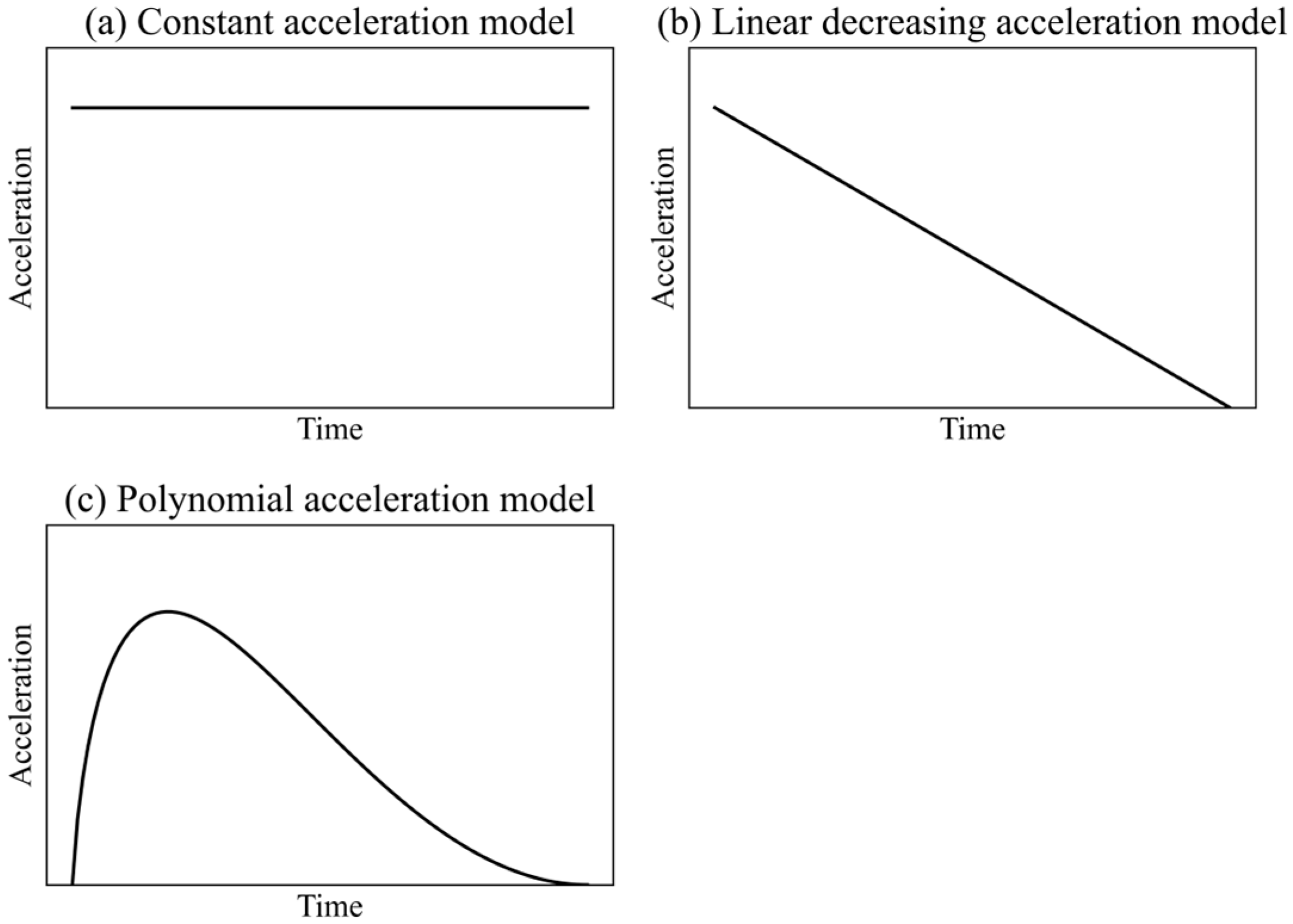
Three existing acceleration profile models, i.e., constant acceleration model, linear decreasing acceleration model, and polynomial acceleration model, can hardly accurately describe or explain a vehicle’s acceleration curves. Figure 6 shows the three acceleration profile models.

Constant acceleration profile model: The constant acceleration profile model describes the boundedness of the vehicle’s acceleration. Incorporating the profile model into the traffic flow model can reproduce the void in vehicles’ trajectories and the capacity drop phenomenon [9]. In addition, a constant acceleration profile exists in some eco-driving strategies [39,40] to increase the tractability of the strategies. However, the constant acceleration profile model cannot describe the jerk’s boundedness, and it is also not a comfortable driving style.

Linear decreasing acceleration profile model: The linear decreasing acceleration profile model is a branch of the present acceleration profile model. However, the linear decreasing acceleration profile cannot describe two bounded conditions caused by maximum jerk and maximum acceleration. Some of the literature [20,22] held that the linear decreasing acceleration model cannot accurately describe the acceleration. In reality, the last acceleration segment can be described by a linear decreasing function considering the “zero-jerk” condition at the two ends of the segment.

Polynomial acceleration profile model: The Polynomial model can describe the “zero-jerk” condition of the acceleration curves, and it can also describe the bounded condition of a maximum jerk. However, it cannot describe the bounded condition of maximum acceleration. In addition, the polynomial acceleration profile model is just a model of a fit curve, which cannot explain how the acceleration curve forms. Thus, it is also difficult to extend to different acceleration scenarios without refitting.

4.6. The Proposed Acceleration Model Coupled with Energy Consumption

In the above content, we produce the vehicle’s acceleration curves considering the driver’s pursuit of mobility and driving comfort. For the human-driven vehicle trajectory, drivers do not always consider energy consumption because they can hardly sense the energy consumption with real-time velocity and acceleration variation.

In this subsection, we investigate the optimal acceleration curve considering energy consumption. Energy consumption models are incorporated into Equation (4). For electric vehicles, energy consumption. i.e., electricity consumption in an acceleration process can be calculated with the vehicle’s motion dynamic model [41], which is formulated as

$$P(t)=\left(ma(t)+mgcos(\theta ){\displaystyle \frac{C_r}{1000}}(c_{1}v(t)+c_2)\right)\cdot v(t)+\left({\displaystyle \frac{1}{2}}{\rho }_{air}{A}_f{C}_D{v}^2(t)+mgsin(\theta )\right)\cdot v(t)$$

(21)

From Equation (21), we can derive the energy consumption by integrating the power, i.e.,

$$J_{\mathrm{E}}={\alpha }_{\mathrm{E}}\left({\displaystyle {\int }_{t_0}^{t_f}P}(t)dt+{\displaystyle \frac{1}{v_f}}\left(L-{\displaystyle {\int }_{t_0}^{t_f}v}dt\right)P_c\right)$$

(22)

where $P_c$ is the vehicle’s constant power with $v_f$. Here, $m$ is the vehicle mass, $g$ is the gravitational acceleration, $\theta$ is the road grade, $c_1$ and $c_2$ are the rolling resistance parameter, ${\rho }_{air}$ is the air mass density, $A_f$ is the frontal area of the vehicle, and $C_D$ is the aerodynamic drag coefficient of the vehicle.

When we integrate the energy consumption into the total cost function Equation (4), the total cost is modified as

$$J={\beta }_1{t}_f+{\displaystyle {\int }_{t_0}^{t_f}(}{\beta }_{2}v+{\beta }_{3}a+{\beta }_4{a}^2+{\beta }_{5}av+{\beta }_6{v}^2+{\beta }_7{v}^3)dt$$

(23)

Proposition 2.

Integrating electric vehicle energy consumption makes the third segment of the acceleration curves become convex.

Proof. 

According to Equations (21)–(23), after the electric vehicle’s energy consumption is considered, ${\beta }_2$ is reformulated as

$${\beta }_2=-{\alpha }_{\mathrm{E}}\left({\displaystyle \frac{P_c}{v_f}}-mgcos(\theta ){\displaystyle \frac{C_r}{1000}}{c}_2\right)-{\displaystyle \frac{{\alpha }_{\mathrm{VOT}}}{v_f}}<-{\displaystyle \frac{{\alpha }_{\mathrm{VOT}}}{v_f}}$$

(24)

According to Equation (21), ${\beta }_6>0$ and ${\beta }_7>0$. According to the properties of the optimal control problem, the Hamiltonian is also an affine function of the control input $j$. The optimal value in the singular arc $j_s$ is formulated as

$$j_s={\displaystyle \frac{{\beta }_2}{2{\beta }_4}}+{\displaystyle \frac{2{\beta }_{6}v+3{\beta }_7{v}^2}{2{\beta }_4}}$$

(25)

With the increase of velocity, $j_s$ increases; thus, the third segment of the acceleration curve is convex. □

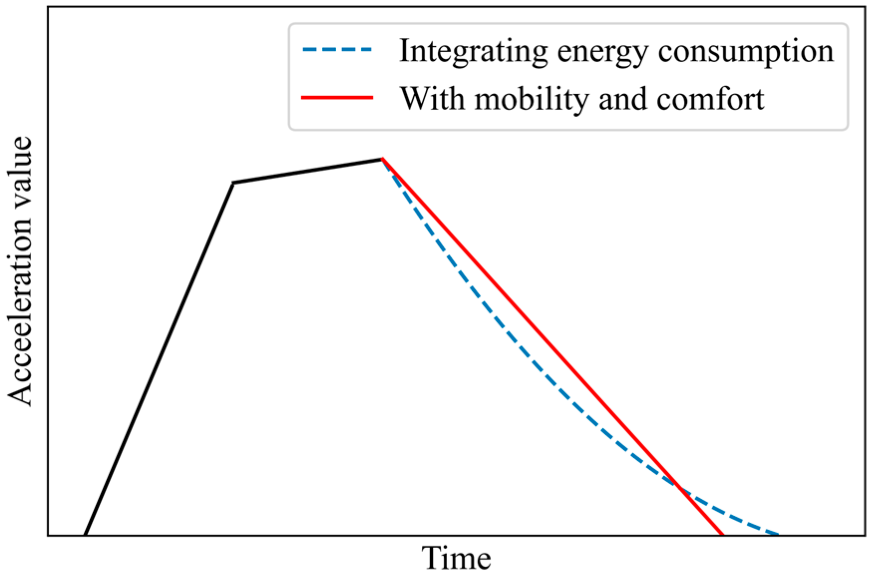
Proposition 2 indicates that considering an electric vehicle’s energy consumption changes the shape of the acceleration profile in the third segment. A sketch that describes the properties is shown in Figure 7.

The derived acceleration profile has a lower derivative at the beginning of the third segment than the corresponding value when electric consumption is not considered. But jerk increases with speed. From Equation (25) and Figure 7, it is easily found that the acceleration value should decrease sharply at the beginning of the third segment, and then the jerk increases to ensure the value of acceleration is relatively low when the vehicle’s velocity is high.

Integrating the electric vehicle’s energy consumption changes the acceleration curves derived by the proposed acceleration profile model. The reasons for the changes are (i) when the vehicle’s velocity is not high, the electric vehicle’s energy consumption mainly depends on the acceleration; therefore, the acceleration should decrease sharply. (ii) When the velocity is high, an electric vehicle’s energy consumption is mainly dependent on the vehicle’s speed. The increase of jerk in the third segment decreases the length of the period when the velocity is close to $v_f$.

5. Discussion

5.1. Predicting the Discharge Rate of Bottleneck

In [9], the discharge rate of a bottleneck is influenced by the bounded acceleration. Also, the queue discharge rate in signalized intersections is dependent on the acceleration curves of all vehicles [10]. In the above literature, the bounded acceleration is assumed as constant, linearly decreasing bounded acceleration, or [10] using a modified cell transmission model to describe the acceleration’s influence on the discharge rate with field data. The results and conclusions of the above literature bring insights into understanding the properties and the evolution of the bottleneck’s discharge rate. However, it cannot accurately describe and predict the discharge rate in a bottleneck with a specific platoon of vehicles.

With the help of the present acceleration profile model, each vehicle’s acceleration curves can be derived with information on the vehicle’s acceleration trajectories upstream of the intersection by vehicle-to-infrastructure technologies. The void of the trajectories of a platoon of vehicles can be calculated; thus, the discharge rate of the bottleneck is derived.

5.2. Providing Information for the Eco-Driving Strategies

It is necessary to pre-acquire the discharge rate of the intersection when implementing eco-driving strategies in a mixed traffic flow with HVs and CAVs. For example, Yang et al. [42] assumed that the vehicle would accelerate or decelerate at a constant throttle level in the signalized intersection, and they incorporated the constant acceleration profile model into the LWR model to predict the evolution of the traffic flow in the downstream of the controlled vehicles. This acceleration profile is uncomfortable for drivers and passengers from the present study.

6. Conclusions

This study introduces a framework that combines optimal control theory with real-world data to model vehicle acceleration profiles. The acceleration curves are divided into three segments: one constrained by maximum jerk, another governed by maximum acceleration, and a third focused on ensuring driving comfort. However, these segments may not coexist within a single acceleration process unless the gap between the target and initial vehicles exceeds a certain threshold. The study also compares the derived acceleration profile with existing models. Additionally, the framework is used to generate energy-efficient acceleration profiles, resulting in the convexity of the third segment within the acceleration curves.

Through analyzing the vehicle’s acceleration properties using the framework’s analytical solution, the study provides insights into how acceleration profiles vary across different driving scenarios. These findings are instrumental in developing machine learning models that replicate human driving behavior during acceleration. Moreover, the derived acceleration properties can support the design of eco-driving strategies, especially at signalized intersections. The anticipation of upcoming queue dynamics within intersections can be accurately predicted by utilizing the acceleration properties derived from short-term trajectory data that is detected by roadside units in the upstream link of the intersection.