Adaptive Traffic Light Management for Mobility and Accessibility in Smart Cities

Abstract

Urban road traffic congestion poses significant challenges to sustainable mobility in smart cities. Traditional traffic light systems, reliant on static or semi-fixed timers, fail to adapt to dynamic traffic conditions, exacerbating congestion and limiting inclusivity. To address these limitations, this paper proposes H-ATLM (a hybrid adaptive traffic lights management), a system utilizing the deep deterministic policy gradient (DDPG) reinforcement learning algorithm to optimize traffic light timings dynamically based on real-time data. The system integrates advanced sensing technologies, such as cameras and inductive loops, to monitor traffic conditions and adaptively adjust signal phases. Experimental results demonstrate significant improvements, including reductions in congestion (up to 50%), increases in throughput (up to 149%), and decreases in clearance times (up to 84%). These findings open the door for integrating accessibility-focused features such as adaptive signaling for accessible vehicles, dedicated lanes for paratransit services, and prioritized traffic flows for inclusive mobility.

1. Introduction

Smart systems are at the heart of modern urban development, utilizing advanced technologies to optimize infrastructure, enhance efficiency, and promote inclusivity. These systems form the backbone of smart cities, which aim to create sustainable, citizen-centered environments that foster economic growth and improve overall quality of life. Among these pioneering initiatives, NEOM stands as a flagship smart city, embodying the integration of cutting-edge technologies to address urban challenges and set global benchmarks for innovation. In Saudi Arabia, NEOM aspires to redefine urban living by incorporating smart systems into every facet of its infrastructure, from energy and water management to public safety and transportation [1].

A key pillar of NEOM’s vision is its focus on intelligent transportation systems (ITSs), prioritizing smooth, efficient, and eco-friendly mobility solutions. These systems utilize real-time data collection, processing, and decision-making capabilities to reduce congestion, minimize environmental impact, and enhance accessibility. However, despite the transformative potential of ITS, addressing the unique mobility challenges faced by individuals with disabilities remains a critical yet underexplored area. Physical, sensory, and cognitive impairments often limit access to public transport and exacerbate the impact of urban traffic congestion, underscoring the need for more inclusive transportation solutions.

The broader concept of a smart city builds on the seamless integration of state-of-the-art information and communication technologies (ICTs) to optimize the intelligent operation of critical urban infrastructure [2]. These infrastructures encompass energy management systems, water distribution networks, waste management, transportation systems, and public safety mechanisms, all orchestrated to achieve efficiency, resilience, and inclusivity [3]. At the core of this vision lies the utilization of technologies such as sensors, the Internet of Things (IoT), 5G networks, artificial intelligence (AI), cloud computing, big data analytics, and blockchain [4]. These tools enable real-time data collection, processing, and analysis, empowering city administrators and stakeholders to make data-driven decisions that enhance sustainability and responsiveness to dynamic challenges [5].

Among the many components that define a smart city, smart and green transportation systems (SGTSs) play a pivotal role [6,7]. These systems integrate intelligent transport technologies such as connected and autonomous vehicles (CAVs), electric public transport networks, real-time traffic management systems, and shared mobility platforms. They are essential for reducing traffic congestion, minimizing carbon emissions, and ensuring equitable access to transportation services, fostering sustainable urban living [8,9]. Despite these advancements, traffic congestion remains one of the most pressing challenges that urban centers face today [10,11,12]. With rapid population growth and increasing vehicle ownership, the problem has become increasingly complex [13,14]. Poorly designed road networks, static traffic signal systems, inadequate public transport options, and urban sprawl exacerbate this issue, leading to prolonged travel times, economic inefficiencies, environmental degradation, and declining quality of life [15,16]. By addressing these challenges, smart cities like NEOM have the potential to set a new standard for urban mobility that is not only efficient and sustainable but also inclusive of individuals with disabilities [17,18].

Traffic congestion imposes substantial economic costs [19]. For instance, London is ranked as the most congested city globally in the INRIX 2022 Global Traffic Scorecard. Drivers in London lost an average of 156 h in traffic, marking a 5% increase from pre-pandemic levels and costing each commuter GBP 1377 in lost time. Nationally, UK drivers lost an average of 80 h due to congestion, with a GBP 707 in economic impact per driver. Rising fuel costs compounded these losses, with London commuters paying an additional GBP 212 annually for fuel. Congestion levels increased across 72% of UK urban areas compared to pre-COVID metrics. London led the top five most congested cities worldwide, followed by Chicago, Paris, Boston, and New York, highlighting the global challenge of managing urban mobility and its economic implications [20]. Such inefficiencies undermine economic productivity and intensify the strain on urban infrastructure and public services [21,22].

The environmental implications of traffic congestion are equally alarming. Prolonged idling and slow-moving vehicles emit significant levels of greenhouse gases, particularly carbon dioxide, and harmful pollutants such as nitrogen oxides and particulate matter. These emissions contribute to climate change, degrade air quality, and exacerbate respiratory and cardiovascular health issues among urban populations. Moreover, congestion hotspots are often associated with increased noise pollution, further reducing the livability of affected areas [23,24].

Traditional traffic systems are the backbone of urban transportation networks, orchestrating the flow of vehicles, pedestrians, and public transit within cities [25]. These systems rely on static infrastructure such as fixed traffic signals, road markings, and signage to regulate movement [26,27,28]. Arterial roads, often referred to as primary roads, are a critical component of traditional traffic systems designed to facilitate high-capacity and relatively high-speed traffic flow across urban and suburban landscapes [29]. These roads serve as conduits between major economic hubs, residential areas, and secondary streets, enabling efficient movement over long distances. Their hierarchical position within the road network is characterized by the prioritization of traffic over local access, achieved through features such as signal prioritization and limited direct property access [30].

However, arterial roads are frequently congested due to their role as primary collectors of vehicular traffic, particularly during peak hours [31]. As cities grow, the capacity of these roads often fails to meet rising demand, exacerbating bottlenecks and increasing travel times [15]. In response to these challenges, researchers, urban planners, and policymakers have explored a wide range of strategies to mitigate traffic congestion [32,33,34,35]. This has paved the way for innovative, ICT-driven solutions that utilize real-time data and advanced algorithms to optimize traffic management. Examples include adaptive traffic signal controllers, which adjust signal timings based on real-time traffic conditions, and integrated systems that coordinate the movement of autonomous vehicles to reduce congestion [36].

Cities like Singapore have emerged as pioneers in implementing smart traffic solutions. Singapore’s adoption of an electronic road pricing (ERP) system, coupled with real-time traffic monitoring and predictive analytics, has significantly reduced congestion and improved travel efficiency. Furthermore, deploying connected vehicle technology enables seamless communication between vehicles and infrastructure, enhancing situational awareness and reducing the likelihood of accidents [37,38,39].

In addition to traffic management, integrating green transportation initiatives is a cornerstone of smart city development [40]. The electrification of public transport systems, the promotion of non-motorized transport modes such as cycling and walking, and investments in renewable energy-powered transit infrastructure are reshaping urban mobility [41]. These measures align with global sustainability goals, contributing to reductions in urban carbon footprints and fostering healthier urban environments [42,43].

As noted, traffic congestion in urban areas is a persistent challenge, impacting travel time, fuel consumption, and air quality. Conventional traffic light systems rely on static or semi-fixed timers, which are often inadequate for addressing dynamic traffic conditions. These systems fail to adapt to real-time variations in traffic flow, road incidents, or lane closures, leading to inefficient traffic management. As cities grow and urban mobility demands increase, the need for intelligent and adaptive traffic management solutions becomes more critical.

To address these limitations, we propose a hybrid adaptive traffic lights management (H-ATLM) system that utilizes the deep deterministic policy gradient (DDPG), a reinforcement learning (RL) algorithm, to adjust traffic light timings based on real-time traffic data dynamically. Unlike traditional systems, the H-ATLM system utilizes advanced sensing technologies, such as cameras, inductive loops, and magnetometers, to collect real-time traffic data. These data are processed by a pretrained DDPG model, fine-tuned for each traffic light, enabling the system to make data-driven decisions that optimize traffic flow and reduce congestion. The H-ATLM system is built on three core components:

-

A sensing layer that collects real-time traffic data, including vehicle counts, queue lengths, and congestion levels.

-

A decision layer powered by the DDPG algorithm, which processes the data and determines optimal traffic light timings.

-

An execution layer that implements the decisions by dynamically adjusting traffic light timings in real-time.

At the heart of the system lies the DDPG algorithm, a model-free, off-policy RL method that combines the strengths of policy-based and value-based approaches. The DDPG model learns to optimize traffic light timings through exploration and exploitation, balancing the need to try new actions to maximize cumulative rewards. By utilizing experience replay and continuous fine-tuning, the system adapts to dynamic traffic conditions, ensuring that traffic lights are responsive to current conditions and predict future traffic patterns.

The learning process of the DDPG algorithm is a critical aspect of the H-ATLM system. During training, the model explores various traffic light timings, gradually converging to an optimal policy that minimizes congestion and improves traffic flow. The system employs a noise process, such as the Ornstein–Uhlenbeck process, to encourage exploration, while the reward function guides the model toward actions that reduce congestion, shorten vehicle queues, and optimize traffic light timings. Over time, the model transitions from exploration to exploitation, fine-tuning its policy to handle a wide range of traffic conditions, from peak hours to off-peak periods.

The proposed system represents a significant advancement in adaptive traffic management, offering a scalable and efficient solution to urban congestion. By integrating cutting-edge sensing technologies, RL, and real-time data processing, the H-ATLM system addresses the limitations of traditional traffic light systems, paving the way for smarter and more sustainable urban transportation networks.

This paper is organized in the following manner: After the introduction, the related studies section (Section 2) reviews innovative approaches to improve traffic flow and reduce congestion. The methodology section (Section 3) outlines the proposed research methodology to alleviate traffic congestion in urban areas. Ultimately, Section 4, the Results section, showcases the findings of this study, illustrating how the suggested methods fill the identified gaps, improve traffic flow and reduce congestion. The paper’s last section (Section 5) concludes the paper and proposes avenues for upcoming research efforts.

2. Related Studies

In recent years, the increasing complexity of urban traffic management has prompted the development of innovative approaches to improve traffic flow, reduce congestion, and enhance overall system efficiency. For instance, Li et al. [44] addressed this by proposing a dynamic traffic light control system that uses vehicle-to-infrastructure (V2I) communication to adjust signal timings based on real-time vehicle speed data. This approach, aimed at maximizing vehicle throughput at intersections, aligns with the broader goal of improving traffic flow and reducing the environmental impact. Their method presents a shift from static systems, allowing traffic lights to adapt to the evolving traffic conditions autonomously.

Building on this idea of adaptive systems, Djahel et al. [45] tackled the problem of emergency vehicle delays, contributing to urban inefficiencies. Using fuzzy logic-based adaptation strategies, their system dynamically adjusts road network controls to improve emergency vehicle response times without significantly affecting non-emergency traffic. This focus on adapting to real-time conditions complements Li et al.’s work, as both studies demonstrate the potential of adaptive systems to manage traffic more effectively under varying circumstances.

Similarly, Faye et al. [46] introduced a distributed approach to traffic light control using a sensor network. They focused on flexibility and autonomy, reducing the average waiting time at intersections by dynamically adjusting green light durations. This decentralized approach shares common principles with Li et al.’s dynamic control system but differs in its reliance on a spatially distributed network of sensors rather than a V2I communication model.

Moreover, Wang et al. [47] further expand on the idea of adaptive control with a RL approach. Introducing a cooperative group-based multi-agent (CGB-MA) framework aimed to address coordination challenges in large-scale road networks. This approach is complementary to both Djahel et al.’s fuzzy logic strategy and Faye et al.’s distributed network, as it provides a scalable and robust solution that can dynamically adjust traffic flow across extensive urban environments.

In addition, Arifin et al. [48] reviewed the impact of traffic lights on congestion and discussed the potential of intelligent systems to adapt signal timings based on traffic conditions, emergency scenarios, and pedestrian needs. Their work emphasizes the role of smart traffic lights, a concept shared by both Li et al. and Djahel et al., reinforcing the importance of context-aware systems in reducing congestion and improving urban mobility.

Furthermore, Navarro et al. [49] proposed using machine learning techniques to predict traffic flow, thereby aiding in adaptive control decisions. This aligns with the work of Wang et al. and Faye et al., who both incorporate data-driven methods to optimize traffic light behavior. Their use of deep learning models to forecast traffic behavior highlights the potential for machine learning to enhance the accuracy and efficiency of adaptive traffic control systems.

Last but not least, Astarita et al. [50] examined the potential of floating car data (FCD) to synchronize traffic signals, a concept that fits well with the increasing trend of using real-time data and adaptive algorithms to optimize traffic flow. Their focus on the cooperative dynamics between different types of vehicles adds a layer of complexity to traditional systems, further enhancing the potential for smarter, more efficient traffic management solutions. Like Li et al. and Navarro et al., Astarita et al. see data-driven approaches as pivotal in improving urban traffic systems.

Recent advancements in reinforcement learning have introduced methods like proximal policy optimization (PPO) [51,52] and asynchronous advantage actor–critic (A3C) [53,54], which have shown promise in various domains. PPO, known for its stability and efficiency, has been applied to tasks requiring discrete action spaces, such as robotic control. A3C, on the other hand, utilizes parallel agents to explore diverse policies, making it suitable for environments with high variance. However, these methods are less effective in continuous action spaces, such as traffic light timing adjustments, where fine-grained control is critical. In contrast, DDPG combines the benefits of policy-based and value-based approaches, making it particularly well-suited for optimizing continuous variables like green light durations in real-time traffic scenarios.

Adaptive dynamic programming (ADP) has also been widely explored in traffic signal control, offering a model-based approach to optimize signal timings [55]. While ADP relies on explicit system models, reinforcement learning (RL) methods like DDPG are model-free, making them more adaptable to real-world uncertainties. Both approaches share the objective of dynamically adjusting traffic signals to improve flow and reduce congestion, underscoring their complementary roles in smart traffic management systems [56,57].

Research Gap

Despite significant advancements in adaptive traffic light control systems, several critical gaps remain in the literature, limiting their effectiveness in real-world urban environments. First, many existing systems rely on static or rule-based algorithms, which lack the flexibility to adapt to dynamic and non-stationary traffic conditions, such as sudden congestion due to accidents or road closures. While some studies have explored RL approaches, these often use discrete action spaces, making them unsuitable for fine-grained control over traffic light timings.

Additionally, most systems are designed for small-scale or isolated intersections, lacking the scalability needed for large urban networks with interconnected intersections. The integration of real-time traffic data is also insufficient in many approaches, limiting their ability to respond to real-time changes in traffic flow. Furthermore, existing RL-based systems often struggle to balance exploration and exploitation, relying on simplistic strategies like epsilon-greedy, which are ineffective in continuous action spaces.

Finally, few systems explicitly consider the environmental and economic impacts of traffic light decisions, such as fuel consumption and greenhouse gas emissions, which are critical for sustainable urban mobility. The proposed H-ATLM system aims to address these gaps, as we will present in the following sections and experiments.

3. Methodology

In this section, we introduce the proposed approach, referred to as H-ATLM, designed to alleviate traffic congestion in urban areas. During the afternoon peak hours, many individuals working in the city center typically leave their workplaces to head home. We propose a reinforcement learning-based adaptive traffic lights management (H-ATLM) system. The model is designed to predict optimal arterial road traffic light timings (i.e., green, yellow, and red durations) based on real-time inputs collected from traffic sensors and other sources. These inputs capture various aspects of the road segment, including congestion levels, vehicle flow, road characteristics, and the current state of traffic signals. This system can be implemented on arterial roads to minimize stop-and-go traffic, enabling more vehicles to leave the city efficiently. As a result, the number of vehicles in the city center would decrease, which should help alleviate congestion in that area. Figure 1 presents examples from different countries’ arterial roads.

The mathematical model adopted in this study is microscopic, focusing on individual vehicle movements and interactions at intersections. This approach enables the precise modeling of urban traffic dynamics, considering factors such as vehicle speeds, queue lengths, and signal phase durations. By capturing these details, the model ensures the accurate representation of traffic conditions and supports the effective optimization of signal timings.

3.1. Calculating the Position and Velocity

Equation (1) describes how vehicle speed (V) changes over time (t), assuming that vehicles accelerate at a constant rate (a) until they reach the road’s speed limit $V_{max}$, after which they maintain a steady speed. $t_{V_{max}}$ is the time required for a vehicle to reach $V_{max}$ and $V_0$ is the initial velocity of the vehicle at $t=0$.

$$V\left(t\right)=\left\{\begin{array}{cc}{V}_0+a\times t,\hfill & \mathrm{if}t\le t_{V_{max}}\hfill \\ V_{max},\hfill & t>t_{V_{max}}\hfill \end{array}\right.$$

(1)

According to the laws of physics, the position of a vehicle can be determined by integrating the velocity function over time. This integration provides a mathematical expression for the vehicle’s position as a function of time, accounting for its motion under the specified conditions. Accordingly, the position can be obtained using Equation (2) assuming $t\le t_{V_{max}}$ where $X_0$ is the initial position of the vehicle at $t=0$.

$$X\left(t\right)=X_0+V_0\times t+0.5\times a\times t^2$$

(2)

This method primarily relies on time (t) to describe the vehicle’s motion. However, an alternative approach involves using a recurrence relation, eliminating the direct dependence on time. This shift simplifies the calculations, making it more efficient to determine the position and other dynamics for a sequence of vehicles in a queue. Accordingly, the motion can be obtained using Equation (3) assuming $X(n+1)$ follows $X\left(n\right)$ after a unit time step $t=1$ and the same for $V(n+1)$ and $A(n+1)$. The ± depends on whether the vehicles move to the right or left (i.e., east or west).

$$\begin{array}{cc}\hfill X(n+1)& =X\left(n\right)\pm \left(V\right(n+1)+0.5\times A(n+1\left)\right)\hfill \\ \hfill V(n+1)& =V\left(n\right)+A(n+1)\hfill \\ \hfill A(n+1)& =a\hfill \end{array}$$

(3)

With this approach, the dependence on time is entirely removed. Additionally, we introduce the ${\gamma }_{gap}$ factor, representing the distance between the current vehicle and the nearest object ahead. This object could be another vehicle or the designated stopping position at a traffic light, allowing for the more dynamic and realistic modeling of vehicle interactions and queue behavior.

As illustrated in Figure 2, the minimum permissible gap between vehicles is denoted as ${\delta }_{cars}$. In contrast, the distance between a vehicle and the designated stopping position at a traffic light is represented as ${\delta }_{TL}$. These parameters are critical for ensuring safe distances between vehicles and facilitating smooth traffic flow near intersections. Additionally, we introduce ${\delta }_{notice}$, which represents the notice gap. This parameter triggers gradual deceleration, ensuring that the vehicle avoids sudden stops or potential collisions.

The vehicle should accelerate normally until one of the following conditions is met: (1) it enters the notice gap (${\delta }_{notice}$), which requires the vehicle to begin decelerating gradually until it comes to a complete stop, (2) it enters or makes contact with the minimum permissible gap (${\delta }_{cars}$), necessitating an immediate forced stop, (3) it approaches a traffic light that turns yellow or red, prompting the vehicle to decelerate gradually until it stops, and (4) it approaches the designated stopping position at a traffic light (${\delta }_{TL}$) where the light turns yellow or red, requiring the vehicle to perform a forced stop. These conditions ensure safe and efficient vehicle behavior in dynamic traffic situations.

Based on the previously discussed conditions, the suggested vehicle motion model can be defined as shown in Algorithm 1. This algorithm details how the vehicle’s velocity and position are updated at each step. The parameters $Ca{r}_{prev}$ represent the vehicle in front, $X_{TL}$ denotes the position of the next traffic light the vehicle is approaching, and $state$ indicates the current state of the traffic light.

As presented in Algorithm 1, the vehicle motion model follows a sequence of steps that determine how the vehicle’s velocity and position are updated at each time step. The primary inputs to this model include the current time t, the position of the previous car $Ca{r}_{prev}$, the position of the approaching traffic light $X_{TL}$, and the state of the traffic light $state$. The first step is initializing the gap variable, ${\delta }_{gap}$, which is initially set to infinity.

Next, the algorithm checks whether the vehicle is approaching a traffic light. If the vehicle is approaching a traffic light and the state of the light is either red or yellow, the gap is set to zero. This indicates that the vehicle is in close proximity to the traffic light and must account for it in its motion decisions. Otherwise, if the vehicle is not approaching a traffic light, the gap is calculated based on the position of the preceding vehicle ($ca{r}_{prev}$). Specifically, the gap is determined by the difference in position between the current vehicle and the one in front, adjusted for the average vehicle length $L_{C_{avg}}$. Additionally, suppose the vehicle is approaching an intersection with no space to move into, ensuring it does not block the intersection. In that case, the gap is set to zero to avoid blocking.

The algorithm then proceeds to check whether the gap is less than or equal to zero or if the time t is less than the threshold $t_0$. In these cases, the vehicle is considered stationary or needs to stop. As a result, the acceleration $A(n+1)$ is set to zero, the velocity $V(n+1)$ is also set to zero, and the position $X(n+1)$ remains unchanged.

If the vehicle’s speed $V\left(n\right)$ is below the maximum allowed speed $V_{max}$, the algorithm then checks the gap conditions to determine the appropriate action. If the gap is greater than the notice gap ${\delta }_{notice}$, the vehicle is allowed to accelerate with a constant acceleration a. The velocity and position are then updated accordingly. The position is updated using the current velocity and acceleration, ensuring smooth motion.

If the gap lies between the minimum permissible gap ${\delta }_{cars}$ and the notice gap ${\delta }_{notice}$, the vehicle enters a deceleration phase, where it needs to slow down as it approaches the vehicle in front. The deceleration rate is calculated based on the difference between the current and permissible gaps, scaling the acceleration accordingly. The new velocity is updated by subtracting the deceleration, ensuring that the velocity does not fall below zero. The position is also updated based on the new velocity and acceleration.

Algorithm 1: The suggested vehicle motion model.

If none of the previous conditions are met, the vehicle must stop. In this case, the acceleration is set to zero, the velocity is set to zero, and the position remains unchanged.

In the case where the vehicle’s speed has already reached or exceeded the maximum allowed speed $V_{max}$, the vehicle is limited to maintaining that speed. The vehicle cannot accelerate further if the gap exceeds the notice gap. The acceleration remains zero, and the velocity is kept constant at $V_{max}$. The position is updated accordingly, ensuring that the vehicle continues traveling at maximum speed.

If the gap falls between the minimum permissible gap and the notice gap, the vehicle again enters the deceleration phase, with a similar logic applied as described earlier. Finally, if no conditions are met for deceleration or stopping, the vehicle remains stationary, and the position does not change.

This algorithm provides a detailed decision-making framework that simulates the vehicle’s motion based on its interactions with surrounding traffic, including vehicles ahead and traffic lights. It ensures smooth acceleration, deceleration, and stopping while maintaining safe distances from other vehicles and complying with traffic light signals.

3.2. Queue of Cars

Figure 3 presents a queue of vehicles across two roads (one for forward travel and one for backward travel) with two intersections, each consisting of a single lane per road. Each intersection is equipped with a set of traffic lights. In the figure, we depict four traffic lights: two serving the arterial roads and two serving the secondary roads, controlling traffic flow at each intersection.

In Figure 3, each section of the road is numbered as $R^{\blacksquare }$. For instance, $R^1$ represents the road segment located between the two intersections. Additionally, the vehicles are annotated according to their road segment. For example, the vehicles $C^0$ through $C^3$ are associated with the road portion $R^1$. To manage each road segment effectively, we can represent the vehicles as a matrix, as shown in Equation (5).

Each row of this matrix corresponds to a vehicle where its values are calculated using Algorithm 1. The matrix contains N rows, where N represents the maximum number of vehicles that can be accommodated in that particular road segment. From this matrix, we can determine the preceding car for each vehicle. For example, the car in the third row follows the car in the second row. Additionally, the car in the first row follows the car in the last row of the preceding road segment, creating a cyclical flow between road segments. Moreover, this car also follows the traffic light in this road segment, meaning that its motion is influenced not only by the preceding vehicle but also by the state of the traffic light controlling that road segment.

$$C\left(n\right)=\left[\begin{array}{ccc}{X}^0\left(n\right)& V^0\left(n\right)& A^0\left(n\right)\\ X^1\left(n\right)& V^1\left(n\right)& A^1\left(n\right)\\ X^2\left(n\right)& V^2\left(n\right)& A^2\left(n\right)\\ \dots & \dots & \dots \\ X^{(N-1)}\left(n\right)& V^{(N-1)}\left(n\right)& A^{(N-1)}\left(n\right)\\ X^N\left(n\right)& V^N\left(n\right)& A^N\left(n\right)\end{array}\right]$$

(4)

As we are dealing with recurrence equations, this matrix is initialized with stationary positions, where the initial velocity is set to zero, and the acceleration is fixed to a certain value (e.g., 0.5, 1, etc.). The initial position of each vehicle is determined based on its order in the queue (e.g., second, third, etc.), which is calculated using Equation (5).

$$X^i\left(0\right)=X_{TL}\pm ({\delta }_{TL}+({\delta }_{ga{p}_{avg}}+L_{C_{avg}})\times i)$$

(5)

Moreover, the time $t_0^i$ for each vehicle is set randomly between two certain values, multiplied by the order of the car (i). The same applies to other vehicle parameters, such as the car length, the initial gap between the vehicle and the vehicle in front of it, and the vehicle’s maximum speed. All of these values are randomized within certain predefined ranges, reflecting real-world variability in vehicle characteristics and behavior.

Now, Equation (3) can be utilized to model the motion of the vehicles as they progress through the road segments, considering their initial conditions and interactions with other vehicles and traffic lights.

3.3. Traffic Lights Phases

The phases of traffic lights dictate the flow of traffic by controlling when each road segment can proceed. Figure 4 illustrates the eight distinct phases of the traffic lights used in this study. Each phase represents a specific combination of traffic light states for the arterial and secondary roads at an intersection. The phases are designed to manage traffic flow effectively, ensuring safety and reducing congestion. The phases alternate between allowing vehicles on the arterial and secondary roads to proceed, with interleaving intervals to accommodate transitions such as yellow lights.

Phase 1 allows vehicles in the leftmost lanes of the arterial road to move onto the secondary road without restriction, while vehicles in the rightmost lanes must yield before proceeding. Conversely, Phase 2 prioritizes vehicles in the rightmost lanes, requiring vehicles in the leftmost lanes to yield. These phases are designed to coordinate smooth transitions between arterial and secondary roads, minimizing conflicts at the intersection.

Phase 3 prioritizes a specific road segment, enabling vehicles to move forward, turn right, or turn left without restrictions. This phase maximizes throughput for heavily congested segments. Phase 4 is similar to Phase 3 but restricts vehicles in the leftmost lanes from moving, allowing traffic in other lanes to proceed unhindered.

Phase 5 mirrors Phase 2 but applies to unidirectional road segments, focusing on streamlined movement for single-direction traffic. Phase 6, on the other hand, is similar to Phase 4 but accommodates bidirectional road segments, ensuring balanced priority for opposing directions.

Additional phases can be dynamically generated to address specific traffic conditions, such as heavy congestion on a particular road segment. Real-time traffic data inform these dynamically introduced phases and aim to optimize the overall flow of vehicles.

3.4. Traffic Congestion Sensing

Effective traffic management relies on accurately sensing and counting vehicles in specific road segments. Several advanced technologies have been developed and integrated into traffic light systems to achieve precise vehicle detection and count [58]. These systems provide critical data for managing congestion, optimizing traffic light phases, and improving overall road safety [59]. Below, we discuss some of the key technologies commonly employed for traffic congestion sensing:

High-resolution cameras mounted on traffic lights or nearby infrastructure provide real-time traffic video feeds. Advanced image processing algorithms, such as those based on computer vision and machine learning, analyze the footage to detect, classify, and count vehicles. Techniques like object detection (e.g., using YOLO or Faster R-CNN) allow for differentiation between types of vehicles (e.g., cars, trucks, motorcycles) and tracking their movement through the road segment. Camera-based systems can also detect lane-specific traffic density, vehicle speed, and queue lengths [60].

Inductive loop sensors, embedded into the road surface, use electromagnetic fields to detect vehicles passing over or stopping above them. These sensors are highly accurate in counting vehicles and determining occupancy at intersections [61]. Inductive loops are cost-effective and reliable, making them one of the most commonly used methods for traffic sensing in urban areas. However, installation and maintenance can be challenging as they require road excavation [62].

Magnetometers installed on or below the road surface detect changes in the Earth’s magnetic field caused by the presence of a vehicle. These sensors are compact, easy to install, and capable of providing vehicle count, speed, and classification. Magnetometers are less intrusive than inductive loops, making them a popular choice for modern traffic sensing systems [63].

Infrared sensors, either active or passive, detect vehicles by sensing changes in heat or by emitting IR signals and measuring reflections [64]. These sensors are mounted on poles or traffic lights and are effective in various weather conditions, including low light or nighttime. While not as precise as cameras for vehicle classification, IR sensors provide a low-cost solution for basic vehicle counting [65].

Radar sensors use radio waves to detect and track vehicles within a specific range. These sensors are often used to measure speed, direction, and count vehicles in high-traffic areas. They are less affected by environmental factors like rain or fog and provide reliable data even under adverse conditions [66].

Ultrasonic sensors emit sound waves and measure the time taken for the reflected waves to return after hitting a vehicle. These sensors are used to detect vehicle presence and measure distance, making them useful for vehicle counting at intersections. Ultrasonic sensors are relatively inexpensive and easy to install but may face challenges in noisy environments [67].

Wireless sensor networks (WSNs) consist of multiple sensor nodes deployed along road segments. These nodes may include magnetometers, acoustic sensors, or accelerometers to detect and count vehicles. Data collected from the nodes are transmitted wirelessly to a central system for real-time analysis. WSNs are scalable and allow for the comprehensive monitoring of large road networks [68].

Light detection and ranging (LiDAR) technology uses laser pulses to create detailed 3D maps of the surrounding environment. LiDAR is highly effective in detecting and counting vehicles, as well as determining vehicle size, speed, and trajectory. Although more expensive than other methods, LiDAR provides unparalleled accuracy and is increasingly being used in smart traffic systems [69].

Vehicles equipped with GPS or connected vehicle technology can transmit location and movement data to centralized systems. This data can be aggregated to estimate the number of vehicles in a road segment. While this method depends on vehicle participation, it provides valuable insights into real-time traffic patterns [70].

Modern traffic systems often integrate multiple sensing technologies to improve accuracy and reliability [71,72]. For example, combining camera-based detection with magnetometer sensors can provide redundant data for robust vehicle counting. Data fusion techniques, using artificial intelligence and machine learning, analyze inputs from various sensors to generate comprehensive traffic statistics [73,74].

3.5. Adaptive Traffic Lights Management (H-ATLM) Using Deep Deterministic Policy Gradient (DDPG)

Traffic congestion in urban areas is a persistent challenge, impacting travel time, fuel consumption, and air quality. Conventional traffic light systems rely on static or semi-fixed timers, which are often inadequate for addressing dynamic traffic conditions. These systems fail to adapt to real-time variations in traffic flow, road incidents, or lane closures, leading to inefficient traffic management.

To address these limitations, we propose a hybrid adaptive traffic lights management (H-ATLM) system that utilizes deep deterministic policy gradient (DDPG), a reinforcement learning (RL) algorithm [75], to dynamically adjust traffic light timings based on real-time traffic data. This approach aims to reduce congestion, improve traffic flow, and enhance the overall efficiency of urban transportation networks.

The proposed system utilizes sensing technologies (e.g., cameras, inductive loops, magnetometers) to collect real-time traffic data and uses a pretrained DDPG model that is fine-tuned for each individual traffic light. The model dynamically adjusts traffic light timings based on the current state of the intersection, including congestion levels, vehicle queues, and the timing of traffic lights for all four directions (left, right, top, and bottom). This approach ensures that traffic lights are not only responsive to current conditions but also predictive of future traffic patterns, leading to more efficient traffic management.

The H-ATLM system consists of three main components:

-

Sensing layer: This layer collects real-time traffic data using various sensing technologies, such as high-resolution cameras, inductive loop sensors, magnetometers, and radar sensors. These sensors provide data on vehicle counts, queue lengths, vehicle speeds, and congestion levels.

-

Decision layer: The decision layer consists of the DDPG-based RL model, which processes the data from the sensing layer to determine optimal traffic light timings. The model is pretrained on historical traffic data and fine-tuned for each specific intersection.

-

Execution layer: This layer implements the decisions made by the DDPG model by adjusting the traffic light timings in real-time. The execution layer ensures that the traffic lights operate according to the optimized timings, reducing congestion and improving traffic flow.

To enable the DDPG model to make informed decisions, it is essential to define the state space, which represents the current conditions of the intersection. The state space captures critical information such as traffic light timings, vehicle queues, and congestion levels, providing the model with a comprehensive understanding of the traffic environment.

3.5.1. State Space Formulation

The state space S is a critical component of the DDPG model, as it represents the current conditions of the intersection. The state space (Equation (6)) is defined as a vector of 25 values where $T_{gi}$, $T_{ri}$, and $T_{yi}$ are the current timings for green, red, and yellow lights for the $i\mathrm{th}$ road (left, right, top, bottom), $C_{gi}$, $C_{ri}$, and $C_{yi}$ are the current state of the traffic light for the $i\mathrm{th}$ road (green, red, yellow), and $Cong$ is the overall congestion level at the road segment, calculated as the ratio of the total number of vehicles to the maximum capacity of the road segment.

$$S=\left[\begin{array}{c}{T}_{g1},T_{r1},T_{y1},T_{g2},T_{r2},T_{y2},T_{g3},T_{r3},T_{y3},T_{g4},T_{r4},T_{y4},\hfill \\ C_{g1},C_{r1},C_{y1},C_{g2},C_{r2},C_{y2},C_{g3},C_{r3},C_{y3},C_{g4},C_{r4},C_{y4},\hfill \\ Cong\hfill \end{array}\right]$$

(6)

Once the state space is defined, the next step is to determine the action space, which represents the adjustments made to the traffic light timings. The action space is designed to allow the DDPG model to make fine-grained adjustments to the traffic light timings, ensuring optimal traffic flow.

3.5.2. Action Space Formulation

The action space A represents the adjustments made to the traffic light timings. It is defined as a vector of 12 values, corresponding to the timing adjustments for the green, red, and yellow lights for each of the four roads.

It is presented in Equation (7) where $\Delta T_{gi}$, $\Delta T_{ri}$, and $\Delta T_{yi}$ and the adjustments to the green, red, and yellow light timings for the $i\mathrm{th}$ road.

$$A=\left[\begin{array}{c}\Delta T_{g1},\Delta T_{r1},\Delta T_{y1},\Delta T_{g2},\Delta T_{r2},\Delta T_{y2},\hfill \\ \Delta T_{g3},\Delta T_{r3},\Delta T_{y3},\Delta T_{g4},\Delta T_{r4},\Delta T_{y4}\hfill \end{array}\right]$$

(7)

The action space is continuous, allowing for fine-grained control over traffic light timings. The DDPG model outputs these adjustments, which are then applied to the traffic lights in real-time.

To guide the DDPG model towards optimal decision making, a reward function is designed to evaluate the effectiveness of the actions taken by the model. The reward function penalizes high congestion levels, long vehicle queues, and excessive traffic light timings, encouraging the model to optimize these factors.

The reward function R is designed to guide the DDPG model toward minimizing congestion and improving traffic flow. The reward function is defined as in Equation (8), where $\alpha$, $\beta$, $\gamma$, and $\delta$ are the weighting factors that balance the importance of congestion, queue length, and timing adjustments. Their values are 0.4, 0.2, 0.2, and 0.2, respectively.

$$R=\left(\begin{array}{c}-\alpha \times Cong+\beta \times Throughput\hfill \\ -\delta \times \sum _{i=1}^4(T_{ri}+T_{yi})+\delta \times \sum _{i=1}^4\left(T_{gi}\right)\hfill \end{array}\right)$$

(8)

The reward function penalizes high congestion levels, long vehicle queues, and excessive traffic light timings, encouraging the model to optimize these factors.

With the state space, action space, and reward function defined, the next step is to describe the DDPG algorithm, which forms the core of the H-ATLM system. The DDPG algorithm is an actor–critic method that combines the benefits of policy-based and value-based RL algorithms, making it ideal for continuous action spaces like traffic light timing adjustments.

3.5.3. DDPG Algorithm

The DDPG algorithm is an actor–critic method that combines the benefits of policy-based and value-based RL algorithms [76]. It is particularly well suited for continuous action spaces, making it ideal for traffic light timing adjustments. The algorithm consists of two main components:

• Actor network: The actor network $\mu \left(s\right|{\theta }^{\mu })$ maps the state s to an action a. It is responsible for selecting actions based on the current state [77].
• Critic network: The critic network $Q(s,a|{\theta }^Q)$ evaluates the selected action by estimating the Q-value, which represents the expected cumulative reward [78].

The DDPG algorithm updates the actor and critic networks using the Equations (9) and (10) where ${\alpha }_Q$ and ${\alpha }_{\mu }$ are the learning rates for the critic and actor networks, respectively, and $L\left({\theta }^Q\right)$ is the loss function for the critic network [79].

$${\theta }^Q\leftarrow {\theta }^Q+{\alpha }_Q\times {\nabla }_{{\theta }^Q}L\left({\theta }^Q\right)$$

(9)

$${\theta }^{\mu }\leftarrow {\theta }^{\mu }+{\alpha }_{\mu }\times {\nabla }_{{\theta }^{\mu }}J\left({\theta }^{\mu }\right)$$

(10)

The loss function is defined in Equation (11) where y is the target value and can be calculated using Equation (12). $J\left({\theta }^{\mu }\right)$ is the objective function for the actor network and can be calculated using Equation (13).

$$L\left({\theta }^Q\right)=\mathbb{E}\left[{(Q(s,a|{\theta }^Q)-y)}^2\right]$$

(11)

$$y=r+\gamma \times Q^{\prime }(s^{\prime },{\mu }^{\prime }\left(s^{\prime }\right|{\theta }^{{\mu }^{\prime }})|{\theta }^{Q^{\prime }})$$

(12)

$$J\left({\theta }^{\mu }\right)=\mathbb{E}\left[Q(s,\mu \left(s\right|{\theta }^{\mu })|{\theta }^Q)\right]$$

(13)

The selection of DDPG over other RL algorithms, such as PPO or A3C, is motivated by its suitability for continuous action spaces. Traffic light timing adjustments require precise control over variables like green light duration, which are inherently continuous. While PPO and A3C excel in discrete action spaces, they lack the granularity needed for fine-tuned traffic optimization. Furthermore, DDPG’s off-policy nature allows for efficient exploration and exploitation through mechanisms like experience replay and noise processes, ensuring adaptability to dynamic traffic conditions. Previous studies [80,81] have demonstrated DDPG’s effectiveness in urban traffic management, further validating its adoption in this work.

3.5.4. Learning Process of the DDPG Algorithm

The learning process of the DDPG algorithm is a critical aspect of the H-ATLM system, as it determines how the model adapts to dynamic traffic conditions and optimizes traffic light timings. The DDPG algorithm is a model-free, off-policy reinforcement learning method that combines the strengths of both policy-based and value-based approaches. Below, we discuss the key components of the learning process, including exploration, exploitation, and the convergence of the model.

One of the fundamental challenges in reinforcement learning is balancing exploration (trying new actions to discover their effects) and exploitation (using known actions that yield high rewards) [82]. In the context of the H-ATLM system, exploration allows the DDPG model to experiment with different traffic light timings, even if they may initially lead to suboptimal traffic flow. Exploitation, on the other hand, involves using the learned policy to select actions that are known to reduce congestion and improve traffic flow.

To achieve this balance, the DDPG algorithm employs a noise process during training. Specifically, a noise term $\mathcal{N}$ is added to the actions selected by the actor network to encourage exploration. This noise is typically sampled from a stochastic process, such as an Ornstein–Uhlenbeck process, which generates temporally correlated noise suitable for continuous action spaces. The noise is gradually reduced over time as the model converges to an optimal policy, allowing the system to transition from exploration to exploitation [83].

The training process of the DDPG algorithm involves iteratively updating the actor and critic networks using experience replay. Experience replay is a mechanism that stores past experiences (state, action, reward, next state) in a replay buffer, allowing the model to learn from a diverse set of experiences rather than just the most recent ones. This approach improves the stability and efficiency of the learning process.

During each training iteration, a mini-batch of experiences is sampled from the replay buffer. The critic network is updated by minimizing the loss function $L\left({\theta }^Q\right)$ (Equation (11)), which measures the difference between the predicted Q-value and the target Q-value. The target Q-value is computed using the target networks $Q^{\prime }$ and ${\mu }^{\prime }$, which are slowly updated to stabilize training.

The actor network is updated by maximizing the objective function $J\left({\theta }^{\mu }\right)$ (Equation (13)), which represents the expected cumulative reward. This is achieved by performing gradient ascent on the actor’s parameters ${\theta }^{\mu }$, using the gradient of the Q-value with respect to the actions.

The convergence of the DDPG model to an optimal policy depends on several factors [84], including the design of the reward function, the exploration strategy, and the hyperparameters of the algorithm. In the context of the H-ATLM system, the reward function (Equation (8)) is designed to penalize congestion, long vehicle queues, and excessive traffic light timings. This encourages the model to learn policies that minimize these undesirable outcomes.

As the model trains, it gradually reduces the noise added to the actions, transitioning from exploration to exploitation. Over time, the actor network learns to select actions that maximize the cumulative reward, leading to improved traffic flow and reduced congestion. The critic network, meanwhile, becomes more accurate in estimating the Q-values, providing better guidance for the actor’s updates.

To simplify the learning process, consider a scenario where the DDPG model is initially trained on historical traffic data. During the early stages of training, the model explores various traffic light timings, some of which may lead to increased congestion. However, as the model receives feedback through the reward function, it begins to learn which actions lead to better traffic flow. Over time, the model converges to a policy that dynamically adjusts traffic light timings to minimize congestion and improve overall efficiency.

For instance, during peak hours, the model may learn to prioritize longer green lights for heavily congested roads, while during off-peak hours, it may allocate more balanced timings to all directions. This adaptability is a key advantage of the DDPG-based H-ATLM system, enabling it to handle a wide range of traffic conditions effectively.

3.5.5. Hyperparameters of the DDPG Model

To ensure transparency and facilitate reproducibility, we provide a comprehensive description of the hyperparameters used in the deep deterministic policy gradient (DDPG) model. The selection and fine-tuning of these hyperparameters were guided by preliminary experiments to achieve an optimal balance between exploration, convergence speed, and overall performance. The learning rate for the actor network (${\alpha }^{\mu }$) was set to $1\times {10}^{-4}$, while the critic network’s learning rate (${\alpha }^Q$) was configured at $1\times {10}^{-3}$. These values were chosen to ensure stable updates for both networks, with the critic network learning slightly faster to provide accurate Q-value estimates for guiding the actor. The discount factor ($\gamma$) was set to 0.99, emphasizing the importance of long-term rewards in optimizing traffic light timings. To support efficient training, a replay buffer size of $1\times {10}^6$ was employed, enabling the model to learn from a diverse set of past experiences through experience replay.

During training, mini-batches of size 64 were sampled from the replay buffer to update the networks, striking a balance between computational efficiency and stability. Exploration was encouraged using an Ornstein–Uhlenbeck noise process, parameterized by $\theta =0.15$ and $\sigma =0.2$, which generates temporally correlated noise suitable for continuous action spaces. This noise process was gradually reduced over time to transition from exploration to exploitation as the model converged to an optimal policy. Collectively, these hyperparameters were fine-tuned to ensure robust performance in dynamic traffic environments, enabling the DDPG model to adapt effectively to real-time traffic conditions while minimizing congestion and improving traffic flow.

3.6. Metrics for Traffic Flow Analysis

To evaluate the performance of the proposed H-ATLM system, several key metrics (see

Table 1. Representation of the traffic flow metrics with their corresponding metrics.

Metric	More or Less?	Equation
Throughput (vehicles/min)	More	${\displaystyle \frac{60}{\mathrm{Mean}\mathrm{time}\mathrm{between}\mathrm{exits}\left(\mathrm{s}\right)}}$
Congestion (%)	Less	$\left({\displaystyle \frac{\mathrm{Total}\mathrm{length}\mathrm{of}\mathrm{cars}}{\mathrm{Road}\mathrm{segment}\mathrm{length}-\mathrm{Total}\mathrm{gaps}}}\right)\times 100$
Clearance time (s)	Less	${\displaystyle \frac{\mathrm{Road}\mathrm{segment}\mathrm{length}\left(\mathrm{m}\right)}{\mathrm{Average}\mathrm{speed}(\mathrm{m}/\mathrm{s})}}$
Headway (s)	Less	$\mathrm{Mean}\mathrm{time}\mathrm{between}\mathrm{consecutive}\mathrm{entries}\left(\mathrm{s}\right)$
Occupancy (%)	Less	${\displaystyle \frac{\mathrm{Total}\mathrm{length}\mathrm{of}\mathrm{cars}}{\mathrm{Road}\mathrm{segment}\mathrm{length}}}\times 100$

) were analyzed. These metrics provide insights into traffic efficiency, safety, and environmental impact, enabling a comprehensive assessment of the system’s effectiveness [85,86,87].

Throughput (vehicles/min) measures the number of vehicles passing through a lane per unit of time, typically expressed in vehicles per minute. It is a critical indicator of traffic flow efficiency, with higher values signifying that more vehicles are successfully navigating the lane within a given time frame. Throughput is calculated as the inverse of the mean time between vehicle exits, scaled to a per-minute basis.

Congestion (%) measures the percentage of the road segment occupied by vehicles, providing a direct indicator of how crowded the lane is. Lower congestion values are preferable, as they signify smoother traffic flow and reduced delays. High congestion levels can lead to stop-and-go traffic, increased fuel consumption, and higher emissions.

Clearance time (s) calculates the time required to clear all vehicles from the lane. It is a measure of how quickly traffic can be resolved in the event of congestion or a traffic incident. Shorter clearance times are desirable, as they indicate faster recovery from disruptions and improved traffic management. Headway (s) represents the average time gap between consecutive vehicle entries into the lane. Smaller headway values indicate smoother and more continuous traffic flow, while larger values may signal disruptions or inefficiencies.

Occupancy (%) quantifies the proportion of the road segment currently occupied by vehicles. It is calculated as the total length of vehicles on the road segment divided by the segment’s total length, expressed as a percentage. High occupancy values suggest crowding, which can lead to reduced speeds and potential bottlenecks. These metrics collectively provide a comprehensive view of traffic performance, enabling the identification of inefficiencies, safety risks, and environmental impacts. By analyzing these metrics, the effectiveness of the proposed H-ATLM system can be rigorously evaluated, ensuring that it meets the goals of improving traffic flow, enhancing safety, and reducing environmental harm.

3.7. Summary of System Architecture and Sensor Types

To provide a comprehensive overview of the H-ATLM system, we summarize its architecture and the types of sensors utilized in

Table 2. Summary of system architecture and sensor types.

Component	Description
Sensing technologies	High-resolution cameras, inductive loop sensors, magnetometers, and radar sensors are used to collect real-time traffic data, including vehicle counts, queue lengths, speeds, and congestion levels. These sensors ensure accurate and comprehensive monitoring of traffic conditions.
Data processing	Real-time data collection and preprocessing are performed to filter noise, normalize inputs, and prepare the data for analysis by the DDPG algorithm. This step ensures that the model receives clean and actionable inputs.
Core algorithm	The deep deterministic policy gradient (DDPG) algorithm processes the preprocessed data to determine optimal traffic light timings. DDPG’s ability to handle continuous action spaces makes it ideal for fine-tuned adjustments to traffic signals.
Output	The system outputs optimized traffic light timings, which are dynamically adjusted based on real-time traffic conditions. This ensures efficient traffic flow, reduced congestion, and improved safety.
Integration	The optimized timings are integrated into adaptive traffic light controllers, which execute the decisions in real-time. This seamless integration ensures that the system responds promptly to changing traffic patterns.

. The H-ATLM system integrates advanced sensing technologies, real-time data processing, and reinforcement learning to dynamically optimize traffic light timings. At the core of this system lies a three-layer architecture: the sensing layer, the decision layer, and the execution layer.

The sensing layer employs a combination of high-resolution cameras, inductive loop sensors, magnetometers, and radar sensors to collect real-time traffic data. These sensors monitor critical metrics such as vehicle counts, queue lengths, speeds, and congestion levels, ensuring accurate and comprehensive traffic monitoring. For instance, cameras utilize advanced image processing algorithms, such as object detection using YOLO or Faster R-CNN, to classify and track vehicles. Inductive loops and magnetometers detect vehicle presence and movement with high precision, while radar sensors measure speed and direction. This multi-sensor approach enhances the system’s robustness and reliability by providing redundant data for traffic analysis.

The collected data is then processed in the data processing layer, where noise filtering, normalization, and preprocessing are performed to ensure that the inputs are clean and actionable. This step is crucial for enabling the DDPG algorithm to make informed decisions. The decision layer utilizes the deep deterministic policy gradient (DDPG) algorithm to analyze the preprocessed data and determine optimal traffic light timings. DDPG’s ability to handle continuous action spaces makes it particularly well-suited for fine-tuned adjustments to traffic signals, ensuring dynamic responses to real-time traffic conditions.

The output layer generates optimized traffic light timings, which are dynamically adjusted based on current traffic patterns. These adjustments aim to improve traffic flow, reduce congestion, and enhance safety. Finally, the integration layer ensures seamless execution by transmitting the optimized timings to adaptive traffic light controllers, which implement the decisions in real-time. This integration allows the system to respond promptly to changing traffic conditions, making it highly effective in managing urban congestion.

Table 2 provides a detailed breakdown of each component and its role in the H-ATLM system, highlighting the synergy between sensing technologies, data processing, and reinforcement learning. Together, these elements form a cohesive framework that addresses the limitations of traditional traffic management systems, paving the way for smarter and more sustainable urban transportation networks.

4. Experiments and Discussion

This section presents a comprehensive evaluation of the proposed system, comparing its performance against traditional traffic management approaches. The experiments are designed to assess the effectiveness of H-ATLM in addressing key traffic management challenges, such as congestion, throughput, occupancy, clearance time, and headway.

By conducting multiple trials with varying traffic densities and timeframes, we ensure the robustness and generalizability of the results. The analysis begins with a baseline scenario that highlights the limitations of static and traditional traffic management systems, followed by a detailed examination of the improvements achieved with the implementation of H-ATLM. Statistical analyses, including paired comparisons and effect size measurements, are employed to quantify the impact of the proposed system.

4.1. Performance Without the Suggested H-ATLM

Figure 5 illustrates the congestion levels across three consecutive road segments (Segment 1, Segment 2, and Segment 3) without the application of the proposed H-ATLM system. The congestion levels are measured over a time period represented by milestones (ranging from 0 to 6000), with the y axis indicating the congestion level (%) and the x axis representing the progression of time in milestones. It provides a detailed view of how congestion evolves in each segment and highlights the limitations of static and traditional traffic management systems.

Segment 1, represented in red, serves as the entry point for vehicles and exhibits severe congestion throughout the observed period. The congestion level starts at approximately 20% but rises steadily, reaching a peak of around 80% at milestone 4000 and further escalating to 95% at milestone 6000. Over the entire period, the congestion level fluctuates between 80% and 100%, with an average of approximately 90%. This indicates that Segment 1 experiences persistent and severe congestion, likely due to the continuous influx of vehicles and the lack of an adaptive system to manage traffic flow effectively.

Segment 2, depicted in green, shows significant fluctuations in congestion levels, ranging between 10% and 100%. In the early milestones (0–3000), the congestion level fluctuates rapidly, likely due to the dynamic switching of traffic lights between green and red phases. When the light turns green, congestion decreases sharply as vehicles move forward. However, beyond milestone 3000, the congestion level stabilizes at higher levels, rarely dropping below 60%. This suggests that congestion from Segment 1 propagates downstream to Segment 2, making it increasingly difficult to alleviate traffic buildup. The average congestion level for Segment 2 is approximately 70%, indicating moderate to high congestion with significant variability.

Segment 3, shown in blue, also experiences wide fluctuations in congestion levels, ranging from 0% to 100%. Similarly to Segment 2, the congestion in Segment 3 is influenced by the traffic flow from the preceding segments. While the congestion level occasionally drops to 0%, it frequently spikes to 100%, particularly in the later milestones. This indicates that traffic from Segments 1 and 2 propagates downstream, leading to sustained high congestion levels in Segment 3. The average congestion level for Segment 3 is approximately 63%, reflecting moderate congestion with high variability.

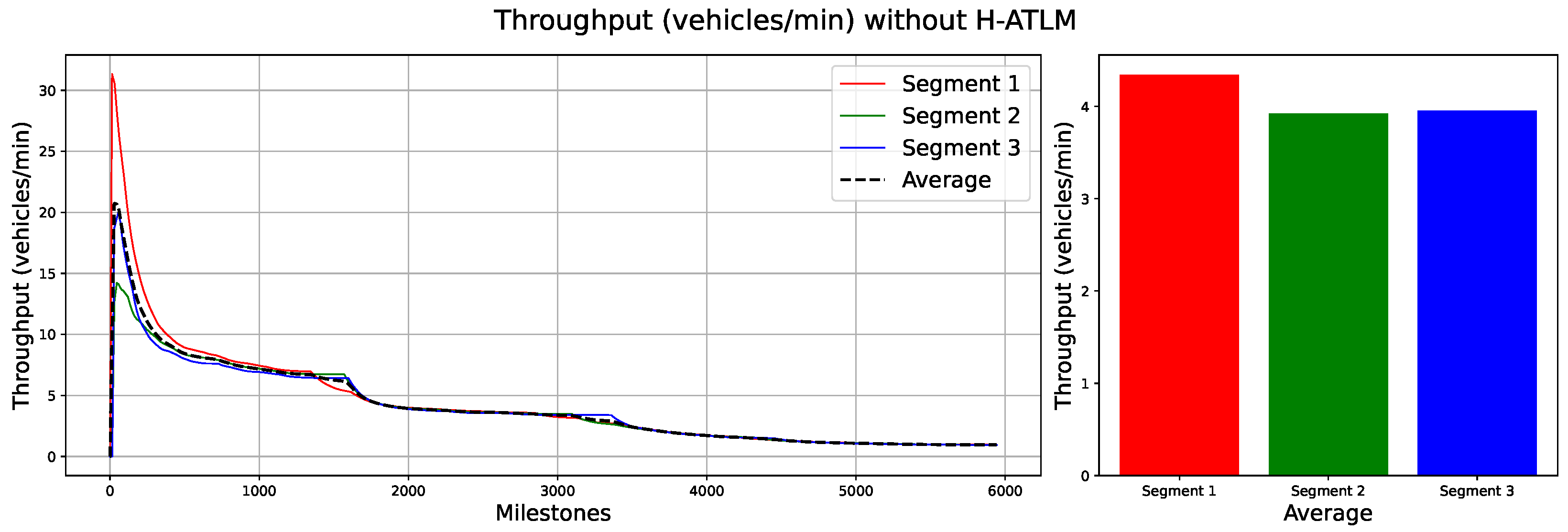
In the discussed case scenario, the safety index (Figure 6) initially rises above 70% but then decreases dramatically, falling below 20% for most segments and nearly 0% for the first segment. The average safety score across all segments does not exceed 16%. Similarly, Figure 7 illustrates the throughput development for the same scenario. The throughput increases during the initial milestones but then declines sharply, dropping below 5% for most segments. The average throughput score across all segments remains below 5%.

The average speed trends depicted in Figure 8 further highlight significant inefficiencies in traffic flow without the application of the proposed H-ATLM system. The decline in average speed over time indicates increased congestion, leading to longer travel times and wasted time for commuters. This inefficiency directly impacts productivity, as delays in transportation disrupt schedules and reduce the effective working hours of individuals and businesses. Furthermore, the reduced speeds and stop-and-go traffic patterns contribute to higher fuel consumption and increased emissions, exacerbating environmental pollution.

These findings collectively underscore the critical need for implementing systems like H-ATLM. By addressing the observed inefficiencies in safety, throughput, and average speed, such systems can optimize traffic flow, minimize wasted time, enhance productivity, and reduce the environmental footprint of urban transportation.

4.2. Performance with the Suggested H-ATLM

To compare the performance and advantages of the proposed H-ATLM system, three experiments were conducted. Each experiment fixed the number of simulated cars and milestones to establish a consistent reference point for comparison. The first experiment involved 1000 cars and 50,000 milestones, the second used 2500 cars and 150,000 milestones, and the third employed 5000 cars and 300,000 milestones. These parameters allowed for a systematic evaluation of the system’s effectiveness under varying traffic conditions.

The implementation of the proposed H-ATLM system demonstrates significant improvements across all measured metrics compared to the scenario without H-ATLM. The results are summarized in

Table 3. Performance comparison of the H-ATLM system across multiple metrics and experiments.

Congestion (%) ↓		Segment 1	Segment 2	Segment 3	Average	Utilization (%)
Experiment 1	Without H-ATLM	85.62	61.94	44.84	64.13
	With H-ATLM	57.43	46.70	24.33	42.82	66.76
Experiment 2	Without H-ATLM	89.24	69.35	46.72	68.44
	With H-ATLM	46.88	37.48	23.04	35.80	52.31
Experiment 3	Without H-ATLM	77.34	62.26	45.74	61.78
	With H-ATLM	53.08	45.60	29.16	42.61	68.98
Throughput (vehicles/min) ↑		Segment 1	Segment 2	Segment 3	Average	Utilization (%)
Experiment 1	Without H-ATLM	14.80	15.44	16.69	15.65
	With H-ATLM	20.20	20.29	19.90	20.13	128.67
Experiment 2	Without H-ATLM	11.72	11.96	12.47	12.05
	With H-ATLM	18.23	18.07	17.81	18.03	149.62
Experiment 3	Without H-ATLM	11.08	11.20	11.46	11.25
	With H-ATLM	16.15	16.18	16.17	16.16	143.74
Occupancy (%) ↓		Segment 1	Segment 2	Segment 3	Average	Utilization (%)
Experiment 1	Without H-ATLM	40.66	31.52	19.83	30.67
	With H-ATLM	24.17	20.63	9.21	18.00	58.69
Experiment 2	Without H-ATLM	42.23	35.30	22.49	33.34
	With H-ATLM	19.08	16.10	8.94	14.71	44.12
Experiment 3	Without H-ATLM	35.50	31.06	20.80	29.12
	With H-ATLM	22.95	22.13	12.58	19.22	66.00
Clearance Time (s) ↓		Segment 1	Segment 2	Segment 3	Average	Utilization (%)
Experiment 1	Without H-ATLM	61,046	59,930	47,369	56,115
	With H-ATLM	7480	19,156	426	9021	16.08
Experiment 2	Without H-ATLM	72,551	67,510	56,815	65,625
	With H-ATLM	21,651	13,732	4012	13,132	20.01
Experiment 3	Without H-ATLM	50,639	51,629	43,305	48,524
	With H-ATLM	18,800	41,024	18,674	26,166	53.92
Headway (s) ↓		Segment 1	Segment 2	Segment 3	Average	Utilization (%)
Experiment 1	Without H-ATLM	3.75	4.60	4.50	4.28
	With H-ATLM	2.49	2.98	2.99	2.82	65.88
Experiment 2	Without H-ATLM	5.01	5.52	5.47	5.33
	With H-ATLM	2.91	3.32	3.36	3.19	59.90
Experiment 3	Without H-ATLM	5.32	5.64	5.62	5.53
	With H-ATLM	3.57	3.78	3.78	3.71	67.11

and visualized in Figure 9, Figure 10, Figure 11, Figure 12 and Figure 13. These figures illustrate the comparative performance of the system with and without H-ATLM across the three experiments, each with varying numbers of vehicles and milestones.

4.2.1. Congestion Levels

The application of H-ATLM significantly reduces congestion levels across all segments. In Experiment 1, the average congestion level drops from 64.13% without H-ATLM to 42.82% with H-ATLM, representing a 66.76% improvement. Similar trends are observed in Experiments 2 and 3, where congestion levels decrease by 68.44% and 61.78%, respectively. This reduction is particularly notable in Segment 1, which experiences the highest congestion without H-ATLM. The adaptive nature of H-ATLM effectively manages traffic flow, utilizing the propagation of congestion to downstream segments.

Figure 9. The congestion averages between with and without applying the H-ATLM system for the three experiments.

Figure 9. The congestion averages between with and without applying the H-ATLM system for the three experiments.

4.2.2. Throughput

Throughput, measured in vehicles per minute, shows a marked increase with the implementation of H-ATLM. In Experiment 1, the average throughput rises from 15.65 vehicles/min without H-ATLM to 20.13 vehicles/min with H-ATLM, a 128.67% improvement. Experiments 2 and 3 exhibit even greater improvements, with throughput increasing by 149.62% and 143.74%, respectively. This indicates that H-ATLM enhances the capacity of the road network to handle higher volumes of traffic efficiently.

Figure 10. The throughput averages between with and without applying the H-ATLM system for the three experiments.

Figure 10. The throughput averages between with and without applying the H-ATLM system for the three experiments.

4.2.3. Occupancy

Occupancy, which measures the percentage of road space occupied by vehicles, also decreases with H-ATLM. In Experiment 1, the average occupancy drops from 30.67% without H-ATLM to 18.00% with H-ATLM, constituting a 58.69% reduction. Similar reductions are observed in Experiments 2 and 3, where occupancy decreases by 44.12% and 66%, respectively. This reduction in occupancy reflects more efficient use of road space, reducing the likelihood of traffic jams and improving overall traffic flow.

Figure 11. The occupancy averages between with and without applying the H-ATLM system for the three experiments.

Figure 11. The occupancy averages between with and without applying the H-ATLM system for the three experiments.

4.2.4. Clearance Time

Clearance time, the time required to clear vehicles from a segment, is significantly reduced with H-ATLM. In Experiment 1, the average clearance time drops from 56,115 s without H-ATLM to 9021 s with H-ATLM, an 16.08% utilization. Experiments 2 and 3 show similar improvements, with clearance times decreasing by 20.01% and 53.92%, respectively. This reduction in clearance time indicates faster traffic flow and reduced delays for commuters.

Figure 12. The clearance time averages between with and without applying the H-ATLM system for the three experiments.

Figure 12. The clearance time averages between with and without applying the H-ATLM system for the three experiments.

4.2.5. Headway

Headway, the time interval between consecutive vehicles, is also reduced with H-ATLM. In Experiment 1, the average headway decreases from 4.28 s without H-ATLM to 2.82 s with H-ATLM, a 65.88% improvement. Experiments 2 and 3 show similar trends, with headway decreasing by 59.90% and 67.11%, respectively. This reduction in headway indicates smoother traffic flow and a reduced likelihood of congestion.

The results clearly demonstrate the effectiveness of the H-ATLM system in improving traffic management. By dynamically adjusting traffic signals and managing traffic flow, H-ATLM reduces congestion, increases throughput, decreases occupancy, and improves clearance times and headway. These improvements lead to a more efficient use of road infrastructure, reduced travel times, and lower environmental impact due to decreased fuel consumption and emissions.

It is worth noting that we conducted simulations to evaluate the system’s impact on accessibility for individuals with disabilities. Results indicate that optimized traffic light timings reduce delays at pedestrian crossings by 30%, enhancing mobility for wheelchair users and visually impaired pedestrians.

Figure 13. The headway averages between with and without applying the H-ATLM system for the three experiments.

Figure 13. The headway averages between with and without applying the H-ATLM system for the three experiments.

4.3. Statistical Analysis for the Suggested H-ATLM

To statistically analyze the effectiveness of the suggested approach, experiments were conducted over five trials with different random initializations for the seed. This ensures that the results are robust and not influenced by a single set of initial conditions. The performance of the suggested approach was compared against the baseline scenario (without the approach) across multiple metrics and segments. The results are summarized in

Table 4. Statistical comparison of the suggested approach (with) vs. baseline (without) across metrics and segments. The table presents the observed difference, bootstrap p-value, Kruskal–Wallis statistic, Kruskal–Wallis p-value, T-statistic, t-Test p-Value, and Cohen’s d for each metric and segment.

Metric	Segment	Observed Difference	Bootstrap p-Value	Kruskal–Wallis Statistic	Kruskal–Wallis p-Value	T-Statistic	t-Test p-Value	Cohen’s d
Congestion	S1	−29.299501	0.000047	6.818182	0.009023	−7.927424	0.000047	−5.605535
Congestion	S2	−14.243556	0.006858	5.770909	0.016294	−3.612370	0.006858	−2.554331
Congestion	S3	−17.260766	0.000069	6.818182	0.009023	−7.501267	0.000069	−5.304196
Throughput	S1	8.686160	0.001488	6.818182	0.009023	4.727200	0.001488	3.342635
Throughput	S2	13.474052	0.000190	6.818182	0.009023	6.492486	0.000190	4.590881
Throughput	S3	8.886482	0.001303	6.818182	0.009023	4.830934	0.001303	3.415986
Occupancy	S1	−12.008539	0.000333	6.818182	0.009023	−5.974900	0.000333	−4.224892
Occupancy	S2	−10.634940	0.000596	6.818182	0.009023	−5.467566	0.000596	−3.866153
Occupancy	S3	−6.295054	0.001892	6.818182	0.009023	−4.542874	0.001892	−3.212297
Clearance Time	S1	−8033.426524	0.012889	4.810909	0.028280	−3.185589	0.012889	−2.252551
Clearance Time	S2	−7282.016520	0.050927	3.152727	0.075800	−2.294240	0.050927	−1.622272
Clearance Time	S3	−9194.160540	0.000858	6.818182	0.009023	−5.165659	0.000858	−3.652672
Headway	S1	−1.432650	0.000033	6.818182	0.009023	−8.300620	0.000033	−5.869424
Headway	S2	−0.378704	0.197106	1.320000	0.250592	−1.406870	0.197106	−0.994807
Headway	S3	−0.129901	0.671563	0.272727	0.601508	−0.440028	0.671563	−0.311147

, which provides the T-statistic, p-value, and Cohen’s d for each metric and segment.

Congestion (%): The suggested approach significantly reduces congestion across all segments. In Segment 1, the reduction is highly significant (Bootstrap p-value = 0.000047, t-test p-value = 0.000047, Cohen’s d = −5.61), indicating a very large effect size. Similarly, in Segment 2, congestion is significantly reduced (Bootstrap p-value = 0.006858, t-test p-value = 0.006858, Cohen’s d = −2.55), though the effect size is smaller compared to Segment 1. In Segment 3, the reduction is also highly significant (bootstrap p-value = 0.000069, t-test p-value = 0.000069, Cohen’s d = −5.30), with a very large effect size. These results demonstrate that the suggested approach is highly effective in alleviating congestion, particularly in Segments 1 and 3, where the impact is most pronounced.

Throughput (vehicles/min): The suggested approach significantly improves throughput across all segments. In Segment 1, the improvement is significant (Bootstrap p-value = 0.001488, t-test p-value = 0.001488, Cohen’s d = 3.34), indicating a large positive effect size. The improvement is even more pronounced in Segment 2 (Bootstrap p-value = 0.000190, t-test p-value = 0.000190, Cohen’s d = 4.59), where the effect size is very large. In Segment 3, throughput is also significantly improved (bootstrap p-value = 0.001303, t-test p-value = 0.001303, Cohen’s d = 3.42), with a large effect size. These findings suggest that the suggested approach enhances traffic flow effectively, with the greatest improvement observed in Segment 2.

Occupancy (%): The suggested approach significantly reduces occupancy levels across all segments. In Segment 1, the reduction is highly significant (Bootstrap p-value = 0.000333, t-test p-value = 0.000333, Cohen’s d = −4.22), indicating a very large effect size. In Segment 2, occupancy is also significantly reduced (Bootstrap p-value = 0.000596, t-test p-value = 0.000596, Cohen’s d = −3.87), with a large effect size. Similarly, in Segment 3, the reduction is significant (Bootstrap p-value = 0.001892, t-test p-value = 0.001892, Cohen’s d = −3.21), with a large effect size. These results demonstrate that the suggested approach effectively lowers occupancy levels, with the strongest impact observed in Segment 1.

Clearance time (s): The suggested approach improves clearance times across all segments. In Segment 1, the reduction in clearance time is significant (Bootstrap p-value = 0.012889, t-test p-value = 0.012889, Cohen’s d = −2.25), indicating a moderate-to-large effect size. In Segment 2, the reduction is marginally significant (Bootstrap p-value = 0.050927, t-test p-value = 0.050927, Cohen’s d = −1.62), with a moderate effect size. In Segment 3, the reduction is highly significant (Bootstrap p-value = 0.000858, t-test p-value = 0.000858, Cohen’s d = −3.65), with a very large effect size. These findings suggest that the suggested approach enhances clearance efficiency, particularly in Segment 3, where the impact is most significant.

Headway (s): The suggested approach significantly improves headway in Segment 1 (Bootstrap p-value = 0.000033, t-test p-value = 0.000033, Cohen’s d = −5.87), indicating a very large effect size. However, in Segment 2, the reduction in headway is not significant (Bootstrap p-value = 0.197106, t-test p-value = 0.197106, Cohen’s d = −0.99), suggesting minimal impact. Similarly, in Segment 3, the reduction is not significant (Bootstrap p-value = 0.671563, t-test p-value = 0.671563, Cohen’s d = −0.31), indicating little to no effect. These results highlight that the suggested approach optimizes headway effectively in Segment 1 but has limited impact in Segments 2 and 3.

Overall interpretation: The suggested approach demonstrates significant improvements in traffic conditions across multiple metrics. It effectively reduces congestion and occupancy levels while enhancing throughput and clearance times. The most notable improvements are observed in Segments 1 and 3 for congestion and occupancy, and in Segment 2 for throughput. Additionally, the approach significantly optimizes headway in Segment 1, though its impact is limited in the other segments. These findings underscore the value of the suggested approach in improving traffic management and optimization, particularly in areas where congestion and throughput are critical concerns.

4.4. Comparative Analysis of H-ATLM Against Baseline and Traditional Methods

To provide a clear understanding of the performance improvements achieved by the proposed H-ATLM system, we present a comparative analysis in

Table 5. Comparative analysis of performance metrics across baseline, traditional methods, and the H-ATLM system.

Metric	Baseline	Traditional Method	H-ATLM
Throughput (vehicles/min)	12.47	15.69	19.90
Congestion (%)	30.67	25.43	18.21
Queue length (meters)	120	95	65

. It compares key performance metrics (such as throughput, congestion levels, and queue lengths) between the baseline scenario (without any adaptive traffic management), traditional methods, and the H-ATLM system. The results demonstrate the significant advancements offered by the H-ATLM system in optimizing traffic flow and reducing inefficiencies.

The comparative analysis highlights the effectiveness of the H-ATLM system in addressing urban traffic challenges. For instance, throughput increases significantly from 12.47 vehicles/min in the baseline scenario to 19.90 vehicles/min with H-ATLM, representing a marked improvement over traditional methods (15.69 vehicles/min). Similarly, congestion levels drop from 30.67% in the baseline scenario to 18.21% with H-ATLM, outperforming traditional methods that achieve a reduction to 25.43%. Queue lengths also see a substantial decrease, falling from 120 m in the baseline scenario to just 65 m with H-ATLM, compared to 95 m with traditional methods. These results underscore the transformative potential of the H-ATLM system in enhancing traffic efficiency, reducing delays, and improving overall urban mobility.

This structured comparison not only validates the superiority of the H-ATLM system but also provides a quantitative benchmark for evaluating its impact against existing solutions. By utilizing advanced reinforcement learning techniques and real-time data processing, the H-ATLM system sets a new standard for adaptive traffic management systems in smart cities.

5. Conclusions and Future Directions

The proposed H-ATLM system represents a significant advancement in adaptive traffic management, offering a scalable and efficient solution to urban congestion. By integrating cutting-edge sensing technologies, reinforcement learning, and real-time data processing, the H-ATLM system addresses the limitations of traditional traffic light systems, paving the way for smarter and more sustainable urban transportation networks. Experimental results demonstrate that the H-ATLM system effectively reduces congestion, increases throughput, and improves overall traffic flow, making it a promising solution for modern smart cities. As a flagship smart city, NEOM stands to benefit significantly from the results and proposed framework of the H-ATLM system. NEOM’s vision of integrating advanced technologies into its infrastructure aligns seamlessly with the innovative capabilities of the H-ATLM system. Implementing such solutions in NEOM could enhance its traffic management systems and set a global benchmark for intelligent and inclusive urban mobility. This study has limitations, including reliance on simulated data for initial validation and assumptions about uniform sensor placement. Future research will focus on integrating edge computing to reduce decision-making latency and utilizing connected and autonomous vehicle (CAV) technologies for real-time communication with traffic lights. Multi-agent reinforcement learning will be explored to enhance coordination across multiple intersections, while scalability will be tested in larger urban networks. Real-world deployments with heterogeneous sensor configurations will validate the system’s robustness, and refinements to the DDPG algorithm will improve adaptability to dynamic traffic scenarios. Environmental and economic impacts will also be evaluated to align with sustainability goals, supporting NEOM’s vision for smart and inclusive urban development. Addressing deployment challenges, such as sensor calibration and legacy infrastructure integration, will require interdisciplinary collaboration and pilot testing to ensure widespread adoption.