Article

Optimal Collector Tilt Angle to Maximize Solar Fraction in Residential Heating Systems: A Numerical Study for Temperate Climates

Faculty of Chemical Engineering and Technology, Cracow University of Technology, Warszawska 24 St, 31-155 Cracow, Poland
*
Authors to whom correspondence should be addressed.
Sustainability 2025, 17(14), 6385; https://doi.org/10.3390/su17146385
Submission received: 11 June 2025 / Revised: 4 July 2025 / Accepted: 9 July 2025 / Published: 11 July 2025

Abstract

The performance of solar thermal systems for space heating and domestic hot water (DHW) production depends on the tilt angle of solar collectors, which governs the amount and seasonal distribution of captured solar radiation. This study evaluates the impact of fixed collector tilt angles on the annual solar fraction (SF) of a solar heating system designed for a typical single-family house located in Kraków, Poland (50° N latitude). A numerical model based on the f-Chart method was employed to simulate system performance under varying collector areas, storage tank volumes, heat exchanger characteristics, and DHW proportions. The analysis revealed that although total annual irradiation decreases with increasing tilt angle, the SF reaches a maximum at a tilt angle of approximately 60°, which is about 10° higher than the local geographic latitude. This configuration offers a favorable balance between winter energy gain and summer overheating mitigation. The results align with empirical recommendations in the literature and offer practical guidance for optimizing fixed-tilt solar heating systems in temperate climates.

1. Introduction

Renewable energy sources and environmental protection play a pivotal role in achieving sustainable development. Growing concerns over fossil-fuel depletion, escalating greenhouse-gas emissions, and rising energy costs have intensified the search for renewable and sustainable heating solutions in the residential sector. Among these, solar space heating stands out as a mature, environmentally friendly technology that leverages freely available solar radiation to satisfy both space-heating and domestic hot water demands. By substituting fossil fuel consumption with solar thermal energy, such systems reduce the extraction of non-renewable resources, curb carbon emissions, enhance energy security, and foster economic growth. Devabhaktuni et al. [1] present a comprehensive overview of the growing role of solar energy in addressing global energy demands, particularly in the context of sustainability, accessibility, and energy security. In temperate and cold climates, however, the inherent intermittency and relatively low intensity of solar irradiance—combined with practical restrictions on collector surface area and storage volume—preclude solar heating from fully replacing conventional systems. Consequently, optimizing system configuration becomes essential.
Two principal parameters govern performance: the total collector aperture area and the capacity of the thermal storage tank. Expanding either increases the solar fraction (the share of heating load met by solar energy), yet spatial and architectural constraints frequently limit such expansions.
An alternative, cost-effective strategy lies in fine-tuning collector orientation and inclination. The tilt angle of a fixed collector array influences both the magnitude and seasonal distribution of incident irradiance. In summer conditions, an increase in the tilt angle of a solar collector results in a decrease in the amount of solar energy.
Numerous studies in the technical literature have addressed the optimization of tilt angles for flat plate solar collectors to improve energy capture and system performance. A foundational and widely cited guideline is provided by Duffie and Beckman [2], who recommend that for maximum annual solar energy collection, the tilt angle of a fixed collector should equal the local geographic latitude and the collector should be oriented toward the equator. For locations in the southern hemisphere, this means a north-facing orientation, while in the northern hemisphere, a south-facing orientation is appropriate. El-Sebaii et al. [3] confirmed experimentally this principle. Supporting evidence is also found in the work of Li et al. [4], who analyzed high-resolution radiation data from Hong Kong and identified an optimal tilt angle of approximately 20° south-facing, which delivered an annual solar yield of over 1598 kWh/m2.
Early empirical models often express the optimal tilt angle as a direct function of latitude ψ, with simple formulas [1,5,6,7,8]. In these formulations, minus values are generally applied in the summer and plus values in the winter to adapt the tilt to seasonal solar altitude changes. These simplified models are particularly useful when a fixed angle is required over long periods. However, more advanced methods have emerged to account for seasonal variations more accurately, using monthly or seasonal constants in correlation with latitude [9].
Chang [10] investigated tilt angle optimization in Taiwan using three radiation datasets: extraterrestrial radiation, empirically predicted global radiation, and long-term observational data. His study found that latitude-based tilt estimations were reliable for extraterrestrial and predicted radiation but needed adjustment in polluted or cloudy environments, where flatter angles were more appropriate. In a related study, Calabrò [11] analyzed regions outside the tropics (36–46° latitude) and confirmed that optimal tilt angles vary significantly by season, especially between winter and summer.
Raptis et al. [12] investigated the optimal tilt angle for solar energy systems by incorporating real atmospheric conditions—specifically cloud cover and aerosol effects—often neglected in traditional models based solely on solar geometry.
Beyond radiation-based criteria, system performance considerations have also influenced tilt angle optimization. Some researchers have focused on grid-connected systems, determining optimal tilt angles under various load conditions—including constant, heating, cooling, and combined heating and cooling loads—by maximizing system efficiency through an optimization factor. Numerous case studies have been conducted globally, confirming the importance of local adaptation. These include analyses for Izmir [13], eight provinces in Turkey [14], Malaysia [15], Dhaka [16], Athens [17], North America [18], India [19], Iran [20], Saudi Arabia [21], Australia [22], Jordan [23,24], and the Mediterranean region [25], highlighting the broad geographical and climatic applicability of such optimization efforts.
Gunerhan et al. [26], focusing on Izmir, emphasized the benefits of monthly adjustment to the tilt angle, showing that dynamic adaptation significantly improves collector efficiency. Can et al. [27] similarly observed that using higher tilt angles in the autumn and winter and lower angles in the summer results in higher solar energy absorption.
Machidon and Istrate [28] analyzed how adjusting collector tilt angles over time improves solar energy harvesting in various European regions. They determined optimum tilt angles for yearly, bi-annual, seasonal, and monthly periods using empirical models and solar radiation estimates.
Mousazadeh et al. [29] provide an extensive review, showing that tracking solutions enhance energy harvest by 10–100%, depending on the time of year and location. Despite these performance improvements, the high cost, added complexity, and increased parasitic energy consumption associated with trackers make them less attractive for small-scale or residential installations [29,30].
Recent studies have increasingly incorporated actual atmospheric conditions, such as cloud cover and aerosols, into tilt optimization analyses. Wei et al. [31], combining experiments and simulations in Isfahan, Iran, found that while optimal tilt angles vary seasonally—lower in spring/summer and higher in autumn/winter—the annual optimum closely aligns with the site’s latitude.
Chinchilla et al. [32] developed models to estimate the annual optimal tilt angle of fixed solar collectors worldwide using only latitude, validated against high-resolution data from 52 stations. Their approach outperformed previous methods in both accuracy and general applicability. Khatib et al. [33] analyzed optimal tilt angles in Dar es Salaam, showing that daily or monthly adjustments could yield up to 5% more energy, while annual optimization offered more modest gains.
Xu et al. [34] addressed high-altitude regions by integrating terrain shading via a viewshed approach, achieving up to 16% higher energy capture compared to conventional methods. Nemalili et al. [35] applied machine learning to nowcast hourly optimal tilt angles, with LSTM models outperforming other algorithms, highlighting the promise of AI for real-time optimization. Finally, Sharma et al. [36] demonstrated that strategic periodic adjustments—three times annually—can significantly enhance energy output and economic returns, even without costly tracking systems.
A substantial body of literature has addressed the influence of collector tilt angle on solar energy systems, ranging from simplified empirical models based on geographic latitude to more advanced simulations incorporating atmospheric conditions and dynamic load profiles. Early works (e.g., [2]) laid the foundation for tilt angle recommendations based on maximizing annual irradiation. Subsequent studies have refined this approach by considering seasonal and monthly adjustments [11,26,28], location-specific optimizations [13,14,15,16,17,18,19,20,21,22,23,24,25], and practical constraints such as storage dynamics and system configuration. More recent research has emphasized dynamic adaptation and hybrid operation [12,27,28], although the focus has remained predominantly on energy yield rather than solar fraction. The present study contributes to this discourse by numerically evaluating the impact of fixed tilt angles on the solar fraction (SF) for combined heating and domestic hot water loads, offering a complementary performance-oriented perspective grounded in thermal system behavior.
The present study employs numerical modeling of the solar fraction of a solar heating system for a standard single-family home in a temperate climate (Kraków, Poland). A spectrum of fixed collector inclinations was simulated to assess their impact on annual energy capture and quantify solar fractions for combined space-heating and domestic hot water loads. The results of our analysis will guide the determination of optimal fixed tilt angles that effectively balance seasonal energy yields, storage dynamics, and load coverage requirements. Ultimately, such guidance will empower designers and homeowners to enhance both the efficiency and sustainability of solar thermal installations.
Section 2 presents a mathematical model detailing the methodology for calculating solar irradiation on the surface of a collector based on data corresponding to a horizontal plane. It also outlines the relationships governing the heat exchanger, the procedure for estimating heating demand using the degree-days method, and the fundamental principles of the f-Chart design method for solar devices. Section 3 provides the input data used in the calculations. The results are discussed in Section 4 and are presented in the form of graphs illustrating solar irradiation, the temporal variation of the f value, and the relationship between the solar fraction and the tilt angle of the collectors for various process parameter values.

2. Mathematical Model

A system for solar heating, schematically illustrated in Figure 1, has been considered.

2.1. Monthly Average Daily Irradiation on a Collector Plane
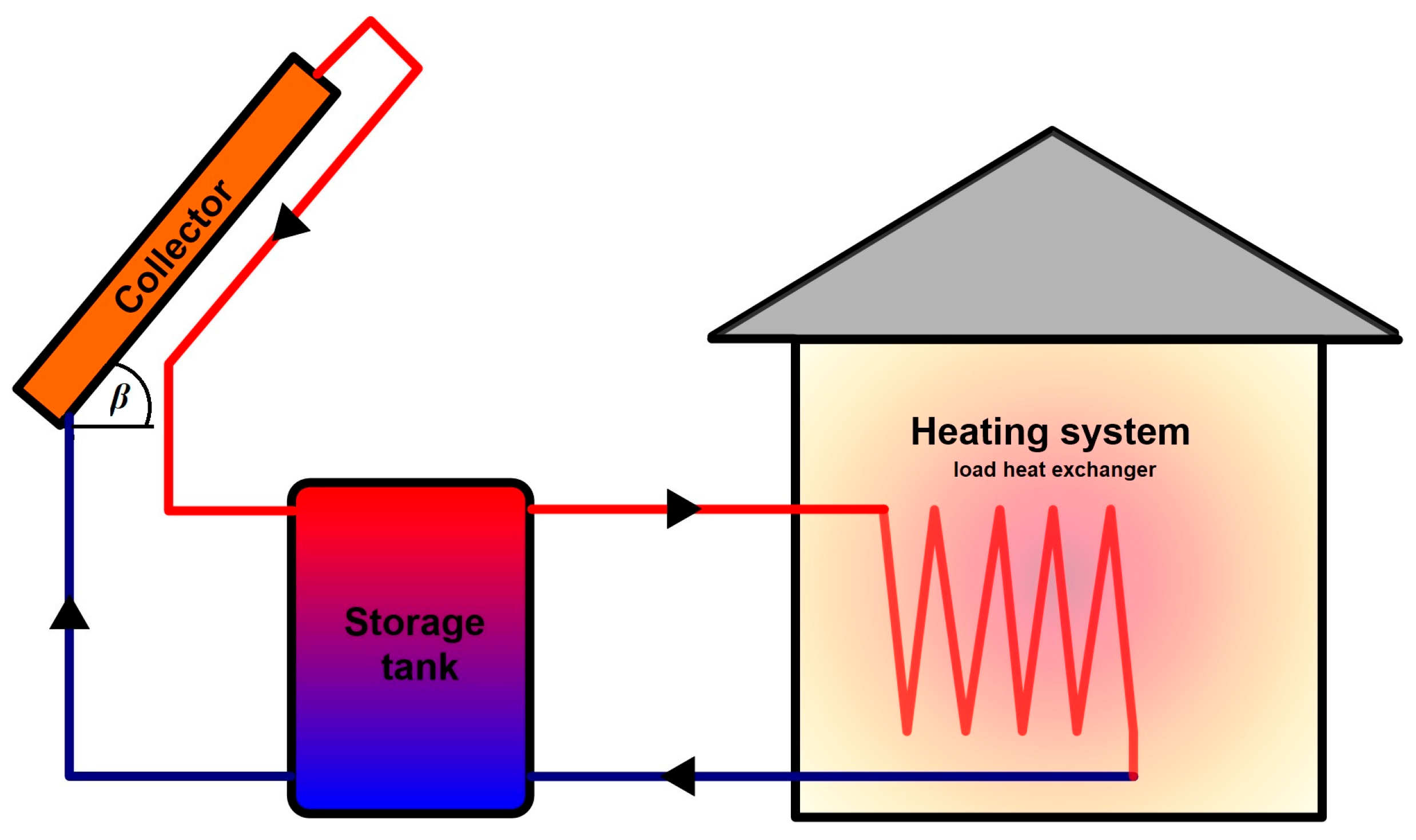
 H ¯ T

It is assumed that the solar collector is located at a geographical latitude ψ, oriented toward true south, and tilted at an angle β with respect to the horizontal plane.
The estimation of the monthly average daily solar radiation incident on the tilted collector surface H ¯ T   [J/m2] is based on the monthly average values of global radiation measured on a horizontal surface H ¯ .
The ratio of these two quantities is calculated using the following formula [2]:
R ¯ = 1 H d ¯ H ¯ R b ¯ + H d ¯ H ¯ 1 + cos β 2 + ρ g 1 cos β 2
Therefore, we obtain the following:
H T ¯ = R ¯ · H ¯  
The values of H ¯ are obtained from meteorological data [37].
The quantity   R ¯ b represents the ratio of the monthly average daily beam radiation on a tilted surface to that on a horizontal surface, as defined by the following relationship [2]:
R b ¯ = cos ψ β cos δ sin ω s + ω s sin ψ β sin δ cos ψ cos δ sin ω s + ω s sin ψ sin δ
The monthly average fraction of diffuse radiation in the total radiation,   H ¯ d / H ¯   , depends on the monthly average value of the atmospheric clearness index   K ¯ T . An empirical polynomial relationship for determining   K ¯ T is presented in the literature [2,38].
The monthly average value of the clearness index     K ¯ T is defined as follows [2]:
K T ¯ = H ¯ H 0 ¯
where H ¯ 0 denotes the monthly average daily extraterrestrial solar radiation. This quantity depends on the day of the year n, the geographical latitude ψ, and the solar declination δ. The relationship is given as follows [2]:
H 0 ¯ = G s c π 1 + 0.033 cos 2 π 365 n cos ψ cos δ sin ω s + ω s sin ψ sin δ
where Gsc = 1367 W/m2 is the solar constant (the solar radiation flux).
The solar declination δ for the n-th day of the year is given by the following [2]:
δ = 23.45 sin 2 π 365 284 + n
The hourly angle of sunset, denoted as ω s , is given by the following [2]:
ω s = cos 1 tan ψ tan δ
The hourly angle of sunset for a tilted surface, denoted as ω s , is given by the following [2]:
ω s = min ω s ,   cos 1 tan ψ β tan δ

2.2. Heat Exchanger

The heat exchanger is characterized by the parameter Z, defined as follows:
Z = ε m ˙ c U b A b
where m ˙ —flow rate of the heating water [kg/s]; c—heat capacity [J/(kgK)]; Ub—overall heat transfer coefficient of the whole building [W/(m2K)]; and Ab—envelope of building area [m2].
For the heat exchanger, it can be assumed that the temperature of the heated air within the room remains uniform throughout the space. Consequently, the effectiveness of the heat exchanger is related to the number of transfer units (NTU) by the following expression:
ε = 1 e x p N T U
where
N T U = U l o a d A l o a d m ˙ c
where Uload—load heat exchanger overall heat transfer [W/(m2K)] and Aload—heat exchanger’s heating surface area [m2].
From the aforementioned relationships, the following is obtained:
Z = 1 e x p N T U N T U · U l o a d A l o a d U b A b
Hence, for a fixed value of the product UbAb and the water flow rate normalized to the heat exchanger surface area m ˙ / A l o a d , the values of Z are proportional to the heat exchanger’s heating surface area A l o a d . Parameter Z typically assumes values in the range from 1 to 3.

2.3. Heat Demand for Heating

The heat supplied to the building, L, is the sum of the heat for space heating, L1, and the heat for domestic hot water heating, L2. The former can be determined from the following relations:
L 1 = U b A b D D m 30.4 · t
The above value pertains to a single day and varies over time in accordance with the fluctuations of the degree days (DDm). The annual heat demand for space heating is obtained by summing the daily values throughout the year.
Σ L 1 = U b A b D D a · t
It is assumed that the annual heat demand for domestic hot water heating constitutes a fraction DHW of the total heat demand. Thus, the average daily heat demand for domestic water heating is as follows:
L 2 = U b A b D D a 365 · D H W 1 D H W · t
In the calculations of the heat demand for space heating, it was assumed that between the 134th and 260th day of the year, the value of L1 is zero.

2.4. f-Chart Model

Calculations based on the f-Chart [2] model are founded on two dimensionless expressions, which, in the standard formulation, are defined as follows:
X = A c F R U L T r e f T a t L
Y = A c F R τ ¯ α ¯ H T ¯ L
In this standard approach, it is assumed that the ratio of the storage tank volume to the collector surface area is V/Ac = 0.075 m3/m2, and that the parameter Z for the load-side heat exchanger equals Z = 2. To eliminate these assumptions, corrected quantities Xc and Yc should be used in place of the expressions X and Y.
X c = X V / A c 0.075 0.25
Y c = Y 0.39 + 0.65   e x p 0.139 Z
According to the f-Chart model, for any given values of V/Ac and Z, the daily fraction of the load supplied by solar energy f, is a function of the dimensionless parameters Xc and Yc. The function is expressed as follows:
f = 1.029   Y c 0.065   X c 0.245   Y c 2 + 0.0018   X c 2 + 0.0215   Y c 3
Since the actual values of the daily solar fraction lie within the interval (0, 1), any calculated f values falling outside this range should be assigned the boundary values f = 0 or f = 1.
The daily energy contribution is the product of f and the daily heating and hot water load L. The fraction of the annual heating load supplied by solar energy (solar fraction) SF is the sum of the daily solar energy contributions divided by the annual load.
S F = Σ f L Σ L
where the summation is taken over the individual days of the year.

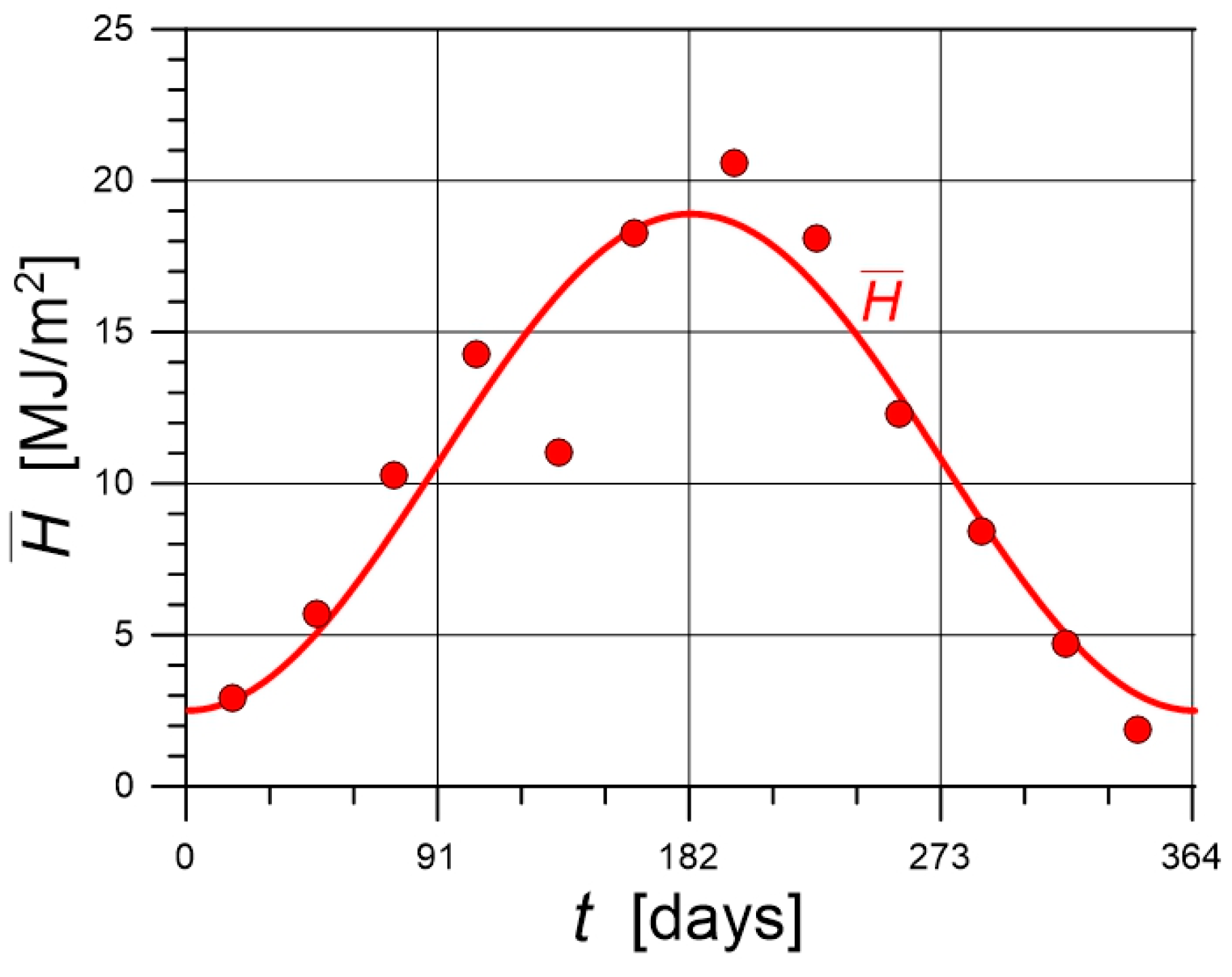
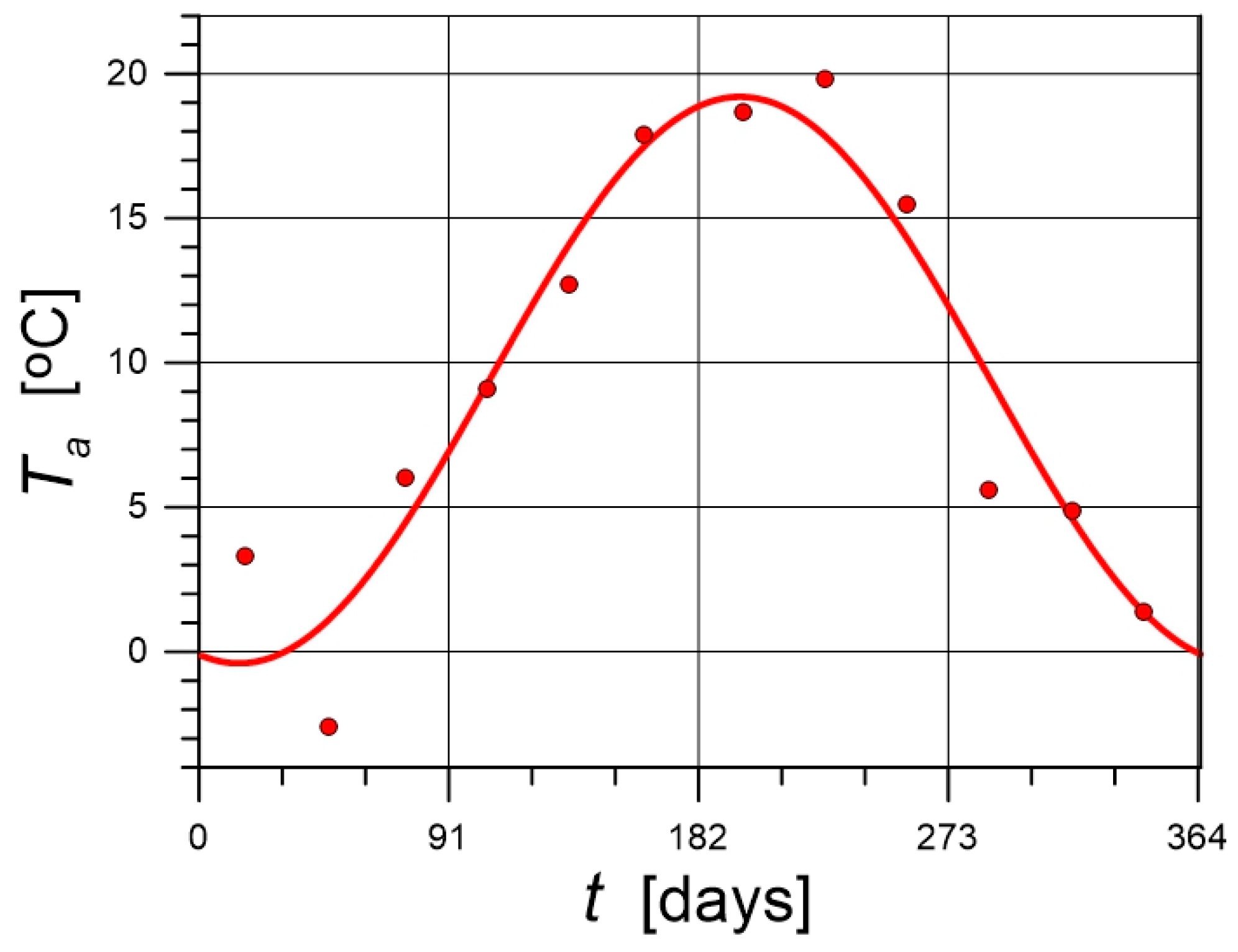
3. Data for Calculations

The calculations were performed using typical meteorological year (TMY) data, obtained from the Photovoltaic Geographical Information System [37]. The monthly average daily solar irradiation on a horizontal surface is shown in Figure 2, where the data points represent measured values, while the solid lines correspond to approximation functions fitted to these experimental data.
By approximating the data, the following relationship was obtained:
H ¯ = 10.7 8.2 · c o s ( ω t 0.0 )
In Figure 3, the temporal variation of the monthly average air temperature is presented, based on meteorological measurements [37]. The solid line represents the trend approximated by the following function, where t denotes the consecutive day of the year.
T a = 9.4 9.8 · c o s ( ω t 0.25 )
The heat demand for space heating depends on the degree-days (DDm). The monthly progression of DDm throughout the year is described by Equation (24), while Figure 4 compares the actual and approximate trends:
D D m = 263 + 281 · c o s ( ω t 0.32 )
The solar installation parameters used in the calculations are presented in Table 1.

4. Results

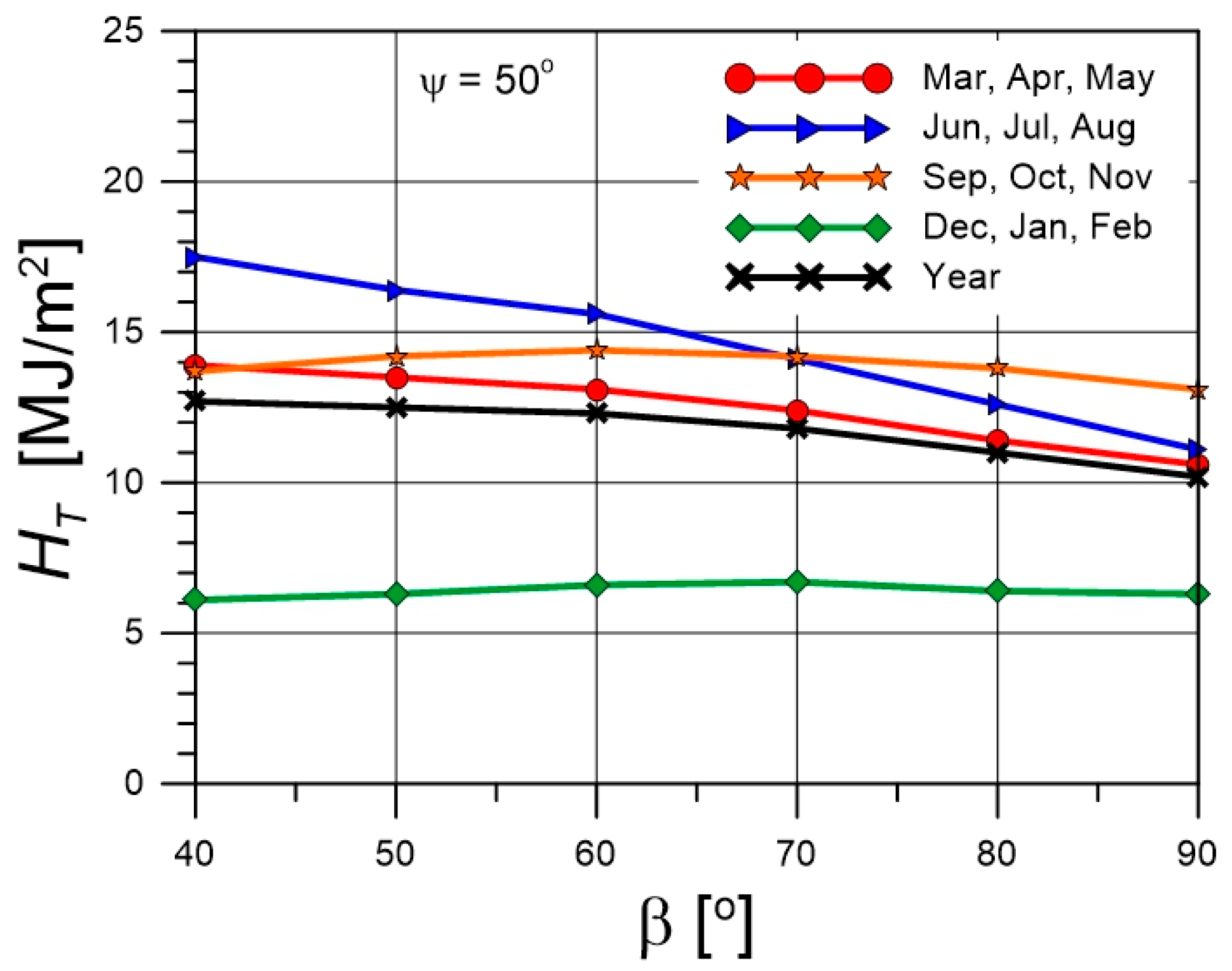
4.1. Solar Irradiation

Determination of the parameter R ¯ , defined by Equation (1), requires knowledge of the collector tilt angle. Since the calculations, outlined below, were conducted for various tilt angles, it was necessary to determine the time-dependent behavior of parameter R ¯ for each value of β. Figure 5 illustrates a representative temporal course of the relationship for β = 40°. The general form of the approximation equations is as follows:
R ¯ = A B · c o s ( ω t P s )
where A, B, and Ps are constants and ω = 2π/365.
The values of the constants in Equation (25) for the specific tilt angles of the collectors are presented in Table 2.
Figure 6 illustrates the temporal variation of daily solar irradiation on the collector surface for tilt angles ranging from 40° to 90°. The values of H T ¯ were calculated according to Equation (3) as the product of H ¯ and R ¯ . The solar irradiation data correspond to locations at a latitude of 50°.
During the summer period, H T values are high for small tilt angles, whereas for larger angles, H T values are lower. In contrast, during the winter period, H T values for the various tilt angles are significantly reduced and exhibit minimal dependence on β.
This is clearly illustrated in Figure 7, which presents the   H T values averaged for each season. During the summer and spring periods, H T decreases with increasing β, whereas in the autumn and winter seasons, the values remain nearly constant.
Additionally, the figure includes a curve depicting the relationship between the annual average   H T and the collector tilt angle. This curve distinctly demonstrates a decline in the annual average   H T as β increases.

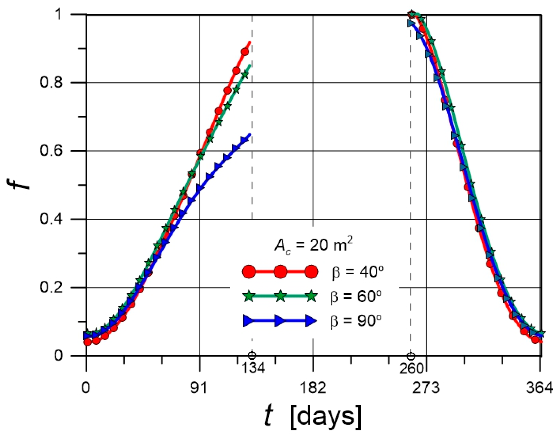
4.2. Temporal Variations of f

Figure 8 and Figure 9 present the simulation results for individual days throughout the year. The f profiles correspond to different tilt angles of the collector. Figure 8 refers to a collector surface area of 20 m2, while Figure 9 pertains to a surface area of 40 m2. The central sections of the graphs represent the summer period, during which space heating is not required. This period spans from the 134th day to 260th day of the year.
Based on the input data used in the simulation, f values rarely reach unity. At the beginning and end of the calendar year, the values of f remain relatively low. For each day of the year, f values are higher when the collector surface area is increased. Differences in the temporal profiles of f for various tilt angles β are primarily observed in the rising segments of the curves. For β = 40°, the f values are generally lower compared to steeper tilt angles, except in May, during which the f values are the highest.
For a tilt angle of 90°, the values of f remain low over a wide time range, particularly from March to May. Although f values are the highest at the beginning and end of the year, their overall contribution to the annual average solar fraction is minimal.
Throughout the entire period under consideration, a tilt angle of 60° yields f values that are either higher than those for other angles or only slightly lower. This suggests that a 60° tilt angle may offer a more favorable performance compared to the other configurations. The above observations apply to both collector surface areas: Ac = 20 m2 and Ac = 40 m2.
Table 3 presents the annual average values of the solar fraction (SF) and solar efficiency (SE). The SF values result from the integration of the function f over the time intervals during which the building is heated using solar energy.
The annual solar efficiency (SE) is defined as the ratio of the amount of solar heat delivered to the building (ΣL) to the total solar irradiation on the collectors, written as follows:
S E = Σ L A c · Σ H T
The numerical values in the table show that SE increases with higher tilt angles, while SF reaches its maximum at β = 60°. Moreover, for identical values of Ac and β, the SE is consistently lower than the SF, then SE < SF.

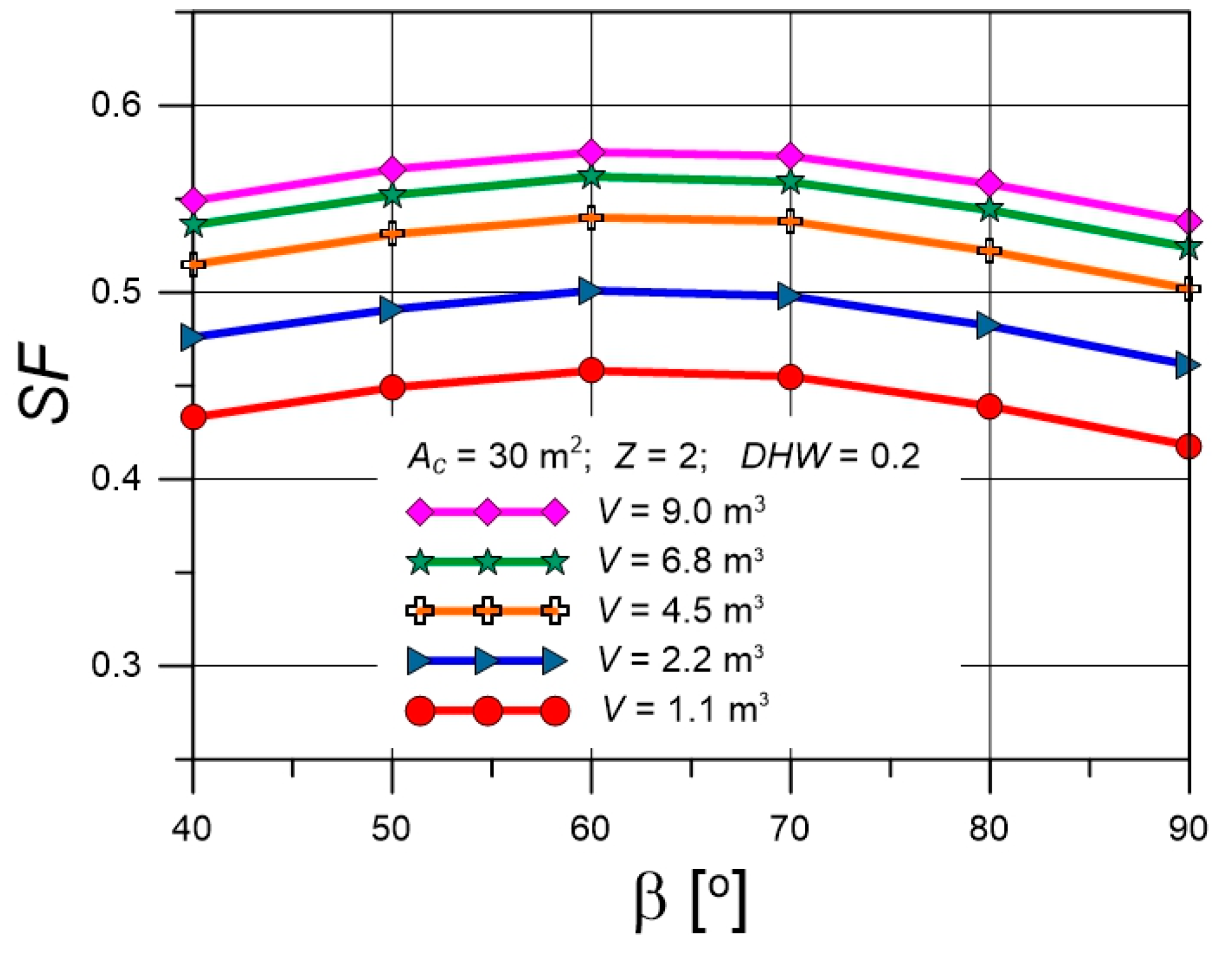
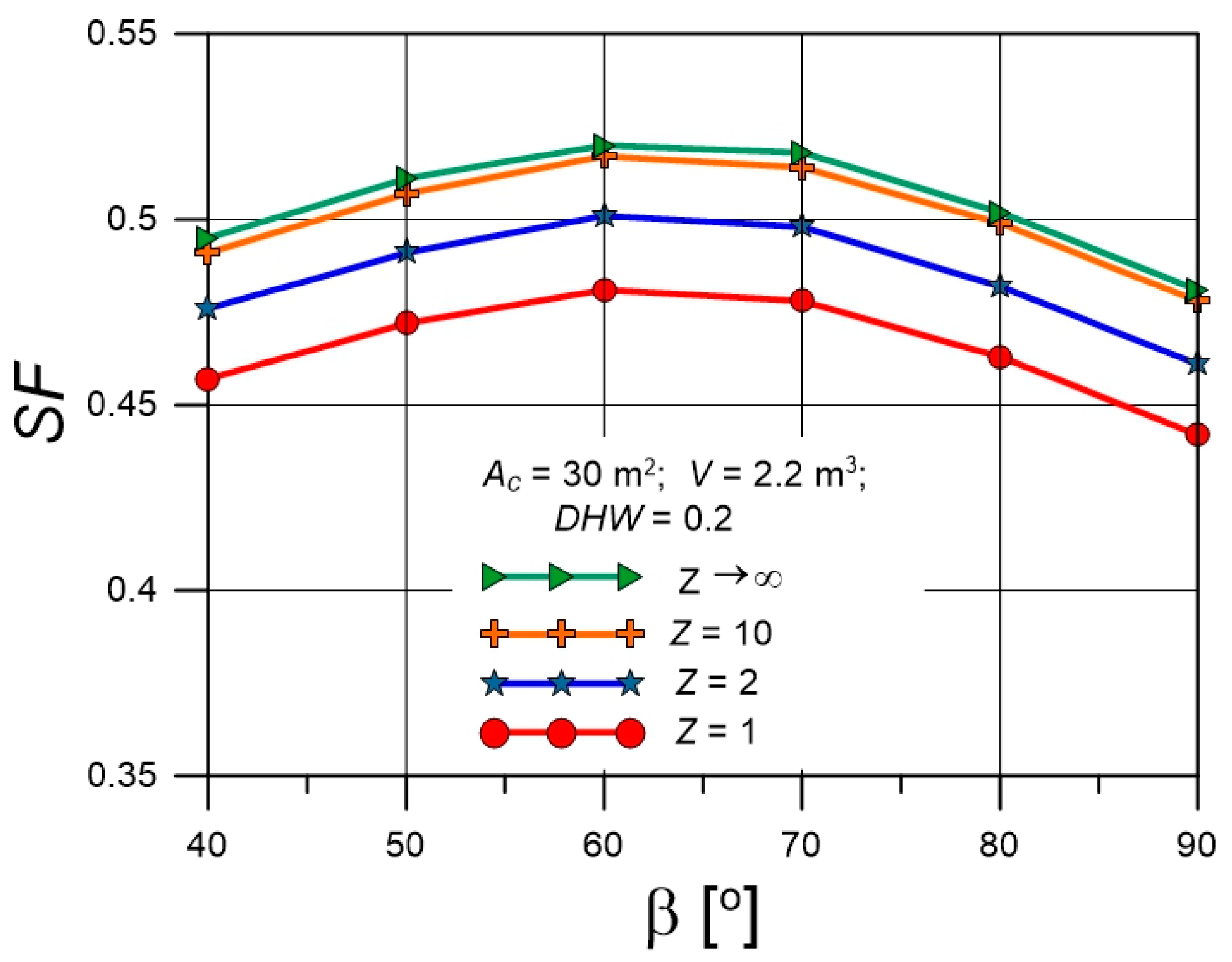
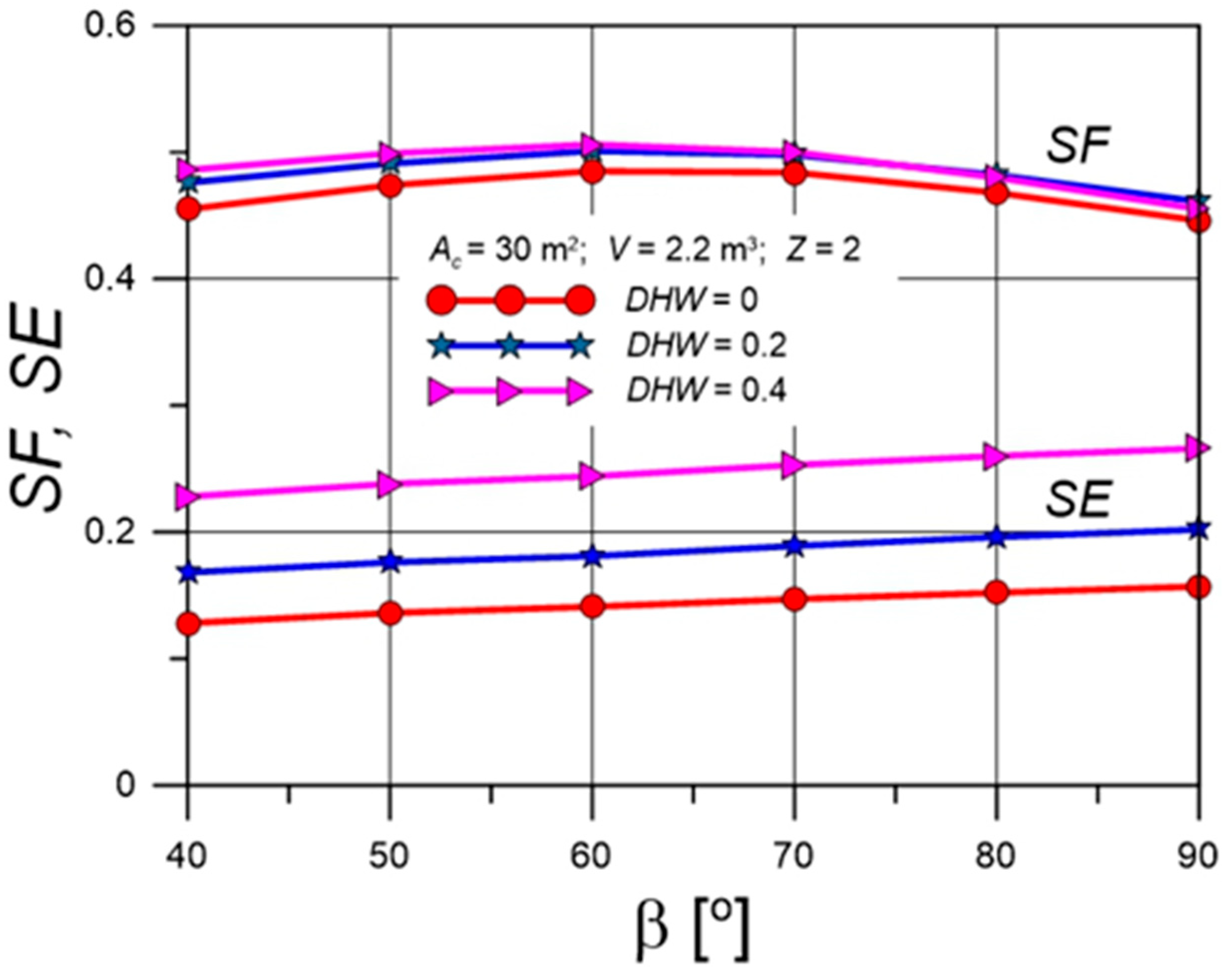
4.3. Solar Fractions for Various Collector Tilt Angles

Figure 10, Figure 11, Figure 12 and Figure 13 illustrate the relationships between the SF, the collector tilt angle β, and various parameters of the solar space heating system: collector surface area Ac, thermal storage tank volume V, the size of the load-side heat exchanger characterized by the parameter Z, and the share of domestic hot water (DHW) in the total thermal energy demand of the building. The values of the remaining parameters are provided in the graph legends or Table 1.
Figure 10 presents the dependence of SF on β for different values of Ac. As Ac increases, the corresponding curve shifts upward. Each curve exhibits a maximum near β ≈ 60°, which is approximately 10° higher than the angle corresponding to the geographic latitude (50°) of the simulation location.
The performance of the solar heating system also depends on the volume of the thermal storage tank. This relationship is illustrated in Figure 11, where each curve corresponds to a different value of V. Each of these curves exhibits a maximum, the position of which is independent of V and occurs at a collector tilt angle of approximately β ≈ 60°.
Figure 12 illustrates the variation of the SF with different values of β and Z. As observed, values of Z above 10 do not lead to further increases in the solar fraction. Moreover, for a given value of Z, all curves exhibit maxima at approximately β ≈ 60°, consistent with the previously presented analyses.
The final parameter under consideration is the quantity DHW, defined as follows:
D H W = Σ L 2 Σ L
where the summation refers to individual days of the year, while L2 denotes the average daily amount of heat consumed for domestic hot water (DHW) production. Domestic hot water is produced with a constant heat demand, regardless of the season, in contrast to heat consumption for space heating. Therefore, a high value of DHW indicates a more balanced heat demand throughout the year as well as a higher overall heat demand.
The increased heat demand is evident in Figure 13 through the behavior of the SE curves. However, the balancing of heat demand does not significantly influence the SF values. The latter reach their maximum at approximately β ≈ 60°, regardless of the value of the DHW parameter.
Theoretically, the optimal difference between the collector tilt angle β and the geographic latitude ψ of the installation site is β − ψ = 0. In practice, it is recommended that β − ψ = 5° for DHW production and 10° for space heating applications [39]. In contrast, Goswami [40] suggests a universal recommendation of β − ψ = 15°, regardless of the application. Therefore, the optimal tilt angle identified in this study is approximately consistent with the values reported in the literature.

5. Conclusions

The efficiency of solar heating systems is influenced by the tilt angle of the collectors relative to the horizontal plane. This is primarily due to the significant impact of surface inclination on the amount of incident solar radiation. From a practical standpoint, however, the key factor is not merely the amount of solar radiation incident on the collector surface but the useful energy ultimately delivered to the heating element. Therefore, this study considered the performance of a complete solar heating installation comprising the solar collector, storage tank, and load-side heat exchanger.
The solar fraction was adopted as the primary performance indicator to assess how collector tilt angle affects the overall system efficiency. To compute this parameter, the f-Chart method was employed.
A set of SF versus tilt angle curves was generated numerically for a range of operating conditions, including variations in collector area, storage tank volume, heat exchanger size, and the proportion of energy allocated to domestic hot water heating relative to the total thermal load. The calculations were based on a typical single-family house located in a temperate climate.
All simulated SFβ plots demonstrate a consistent pattern, featuring an initial ascending section and a subsequent descending section. The peak of each curve corresponds to the most favorable collector tilt angle.
Based on the simulation results, the following guidelines are recommended for selecting the appropriate collector tilt angle:
  • Avoid steep tilt angles approaching 90°.
  • Avoid tilt angles significantly lower than the site’s geographic latitude.
  • For locations at a latitude of approximately 50°, an optimal tilt angle of 60° is recommended.
This proposed optimal tilt angle is based on simulations using meteorological data for Kraków, Poland, and is expected to be applicable to other locations with similar climatic conditions. In general, for geographic latitudes around 50°, the optimal collector tilt angle should be approximately 10° greater than the site’s latitude.
It appears that further research should focus on identifying a relationship that enables the determination of optimal collector tilt angles under varying climatic conditions. To this end, it is necessary to consider a range of geographic latitudes, as well as the temporal profiles of solar irradiation and ambient air temperature. Additionally, future work would greatly benefit from experimental validation to corroborate the theoretical outcomes presented herein.

Author Contributions

Conceptualization, K.K.; methodology, K.K.; software, K.K. and B.K.; validation, K.K. and B.K.; formal analysis, K.K.; investigation, K.K. and B.K.; resources, K.K.; data curation, K.K.; writing—original draft preparation, K.K. and B.K.; writing—review and editing, K.K. and B.K.; visualization, K.K. and B.K.; supervision, K.K. All authors have read and agreed to the published version of the manuscript.

Funding

This research received no external funding.

Institutional Review Board Statement

Not applicable.

Informed Consent Statement

Not applicable.

Data Availability Statement

Dataset available from the author upon request.

Conflicts of Interest

The authors declare no conflicts of interest.

Nomenclature

Abenvelope of building area, m2
Accollectors surface area, m2
cheat capacity, J/(kgK)
DDm, DDamonthly degree-days and annual degree-days, K·day
DHWfraction of energy for domestic hot water heating
fdaily fraction of the load supplied by solar energy
F R collector heat exchanger efficiency factor
FRcollector heat removal factor (including external heat exchanger)
H, H ¯ daily irradiation and monthly average daily irradiation on a horizontal plane, J/m2;
HT, H T ¯


daily irradiation and monthly average daily irradiation on a collector plane, J/m2
L1, L2daily heating load for space heating and hot water respectively, J
Ldaily total heating load, J
m ˙ flow rate of the heating water, kg/s
R ¯ monthly average total radiation on the tilted surface to that on a horizontal surface
SEsolar efficiency
SF(annular) solar fraction
ttime, s or days
Taambient temperature, °C
Trefempirically derived reference temperature (100 °C)
Uboverall heat transfer coefficient of the whole building, W/(m2K)
ULoverall heat transfer coefficient between collector and environment, W/(m2K)
Uloadload heat exchanger overall heat transfer, W/(m2K)
Vvolume of tank, m3
X, Xcdimensionless group and correction dimensionless group (Equations (16) and (18))
Y, Ycdimensionless group and correction dimensionless group (Equations (17) and (19))
Zdimensionless parameter defined by Equation (9)
βcollectors tilt angle, rad or deg
ρgdiffuse reflectance
εeffectiveness of load heat exchanger
Δt time step (=1 day)
(τα) effective transmittance–absorptance product
ψlatitude
ω (=2π/365) frequency, day−1

References

  1. Devabhaktuni, V.; Alam, M.; Depuru, S.S.R.; Green, R.C.; Nims, D.; Near, C. Solar energy: Trends and enabling technologies. Renew. Sustain. Energy Rev. 2013, 19, 555–564. [Google Scholar] [CrossRef]
  2. Duffie, J.; Beckman, W. Solar Engineering of Thermal Processes; John Wiley & Sons Inc.: Hoboken, NJ, USA, 2013. [Google Scholar]
  3. El-Sebaii, A.A.; Al-Hazmi, F.S.; Al-Ghamdi, A.A.; Yaghmour, S.J. Global, direct and diffuse solar radiation on horizontal and tilted surfaces in Jeddah, Saudi Arabia. Appl. Energy 2010, 87, 568–576. [Google Scholar] [CrossRef]
  4. Li, D.H.W.; Lam, T.N.T. Determining the Optimum Tilt Angle and Orientation for Solar Energy Collection Based on Measured Solar Radiance Data. Int. J. Photoenergy 2007, 2007, 85402. [Google Scholar] [CrossRef]
  5. Heywood, H. Operating experience with solar water heating. IHVE J. 1971, 39, 63–69. [Google Scholar]
  6. Löf, G.O.G.; Tybout, R.A. Cost of house heating with solar energy. Sol. Energy 1973, 14, 253–278. [Google Scholar] [CrossRef]
  7. Garg, H.P. Treatise on Solar Energy; Fundamentals of Solar Energy; John Wiley & Sons: New York, NY, USA, 1982; Volume I. [Google Scholar]
  8. Moghadam, H.; Tabrizi, F.F.; Sharak, A.Z. Optimization of solar flat collector inclination. Desalination 2011, 265, 107–111. [Google Scholar] [CrossRef]
  9. Chang, T.P. The Sun’s apparent position and the optimal tilt angle of a solar collector in the northern hemisphere. Sol. Energy 2009, 83, 1274–1284. [Google Scholar] [CrossRef]
  10. Chang, T.P. Study on the optimal tilt angle of solar collector according to different radiation types. Int. J. Appl. Sci. Eng. 2008, 6, 151–161. [Google Scholar]
  11. Calabrò, E. Determining optimum tilt angles of photovoltaic panels at typical north-tropical latitudes. J. Renew. Sustain. Energy 2009, 1, 033104. [Google Scholar] [CrossRef]
  12. Raptis, I.-P.; Moustaka, A.; Kosmopoulos, P.; Kazadzis, S. Selecting Surface Inclination for Maximum Solar Power. Energies 2022, 15, 4784. [Google Scholar] [CrossRef]
  13. Koray, U.; Arif, H. Prediction of Solar Radiation Parameters Through Clearness Index for Izmir, Turkey. Energy Sources Part A 2002, 24, 773–785. [Google Scholar] [CrossRef]
  14. Bakirci, K. General models for optimum tilt angles of solar panels: Turkey case study. Renew. Sust. Energy Rev. 2012, 16, 6149–6159. [Google Scholar] [CrossRef]
  15. Bari, S. Optimum slope angle and orientation of solar collectors for different periods of possible utilization. Energy Convers. Manag. 2000, 41, 855–860. [Google Scholar] [CrossRef]
  16. Ghosh, H.R.; Bhowmik, N.C.; Hussain, M. Determining seasonal optimum tilt angles, solar radiations on variously oriented, single and double axis tracking surfaces at Dhaka. Renew. Energy 2010, 35, 1292–1297. [Google Scholar] [CrossRef]
  17. Kaldellis, J.; Zafirakis, D. Experimental investigation of the optimum photovoltaic panels tilt angle during the summer period. Energy 2012, 38, 305–314. [Google Scholar] [CrossRef]
  18. Moon, S.H.; Felton, K.E.; Johnson, A.T. Optimum tilt angles of a solar collector. Energy 1981, 6, 895–899. [Google Scholar] [CrossRef]
  19. Agarwal, A.; Vashishtha, V.K.; Mishra, S.N. Comparative approach for the optimization of tilt angle to receive maximum radiation. Int. J. Eng. Res. Technol. 2012, 1, 1–9. [Google Scholar]
  20. Jafarkazemi, F.; Saadabadi, S.A.; Pasdarshahri, H. The optimum tilt angle for flat plate solar collectors in Iran. J. Renew. Sustain. Energy 2012, 4, 013118. [Google Scholar] [CrossRef]
  21. Benghanem, M. Optimization of tilt angle for solar panel: Case study for Madinah, Saudi Arabia. Appl. Energy 2011, 88, 1427–1433. [Google Scholar] [CrossRef]
  22. Yan, R.; Saha, T.K.; Meredith, P.; Goodwin, S. Analysis of year-long performance of differently tilted photovoltaics systems in Brisbane, Australia. Energy Convers. Manag. 2013, 74, 102–108. [Google Scholar] [CrossRef]
  23. Shariah, A.; Al-Akhras, M.A.; Al-Omari, I.A. Optimizing the tilt angle of solar collectors. Renew. Energy 2002, 26, 587–598. [Google Scholar] [CrossRef]
  24. Altarawneh, I.S.; Rawadieh, S.I.; Tarawneh, M.S.; Alrowwad, S.M.; Rimaw, I.F. Optimal tilt angle trajectory for maximizing solar energy potential in Ma’an area in Jordan. J. Renew. Sustain. Energy 2016, 8, 033701. [Google Scholar] [CrossRef]
  25. Darhmaoui, H.; Lahjouji, D. Latitude based model for tilt angle optimization for solar collectors in the Mediterranean region. Energy Procedia 2013, 42, 426–435. [Google Scholar] [CrossRef]
  26. Gunerhan, H.; Hepbasli, A. Determination of the Optimum Tilt Angle of Solar Collectors for Building Applications. Build. Environ. 2007, 42, 779–783. [Google Scholar] [CrossRef]
  27. Ertekin, C.; Evrendilek, F.; Kulcu, R. Modeling spatio-temporal dynamics of optimum tilt angles for solar collectors in Turkey. Sensors 2008, 8, 2913–2931. [Google Scholar] [CrossRef] [PubMed]
  28. Machidon, D.; Istrate, M. Tilt Angle Adjustment for Incident Solar Energy Increase: A Case Study for Europe. Sustainability 2023, 15, 7015. [Google Scholar] [CrossRef]
  29. Mousazadeh, H.; Keyhani, A.; Javadi, A.; Mobli, H.; Abrinia, K.; Sharifi, A. A review of principle and sun-tracking methods for maximizing solar systems output. Renew. Sustain. Energy Rev. 2009, 13, 1800–1818. [Google Scholar] [CrossRef]
  30. Tomson, T. Discrete two-positional tracking of solar collectors. Renew. Energy 2008, 33, 400–405. [Google Scholar] [CrossRef]
  31. Wei, D.; Basem, A.; Alizadeh, A.; Jasim, D.J.; Aljaafari, H.A.S.; Fazilati, M.; Mehmandoust, B.; Salahshour, S. Optimum tilt and azimuth angles of heat pipe solar collector, an experimental approach. Case Stud. Therm. Eng. 2024, 55, 104083. [Google Scholar] [CrossRef]
  32. Chinchilla, M.; Santos-Martín, D.; Carpintero-Rentería, M.; Lemon, S. Worldwide annual optimum tilt angle model for solar collectors and photovoltaic systems in the absence of site meteorological data. Appl. Energy 2021, 281, 116056. [Google Scholar] [CrossRef]
  33. Khatib, A.T.; Samiji, M.E.; Mlyuka, N.R. Optimum Solar Collector’s North-South Tilt Angles for Dar es Salaam and their Influence on Energy Collection. Clean. Eng. Technol. 2024, 21, 100778. [Google Scholar] [CrossRef]
  34. Xu, L.; Long, E.; Wei, J.; Cheng, Z.; Zheng, H. A new approach to determine the optimum tilt angle and orientation of solar collectors in mountainous areas with high altitude. Energy 2021, 237, 121507. [Google Scholar] [CrossRef]
  35. Nemalili, R.C.; Jhamba, L.; Kiprono Kirui, J.; Sigauke, C. Nowcasting Hourly-Averaged Tilt Angles of Acceptance for Solar Collector Applications Using Machine Learning Models. Energies 2023, 16, 927. [Google Scholar] [CrossRef]
  36. Sharma, A.; Kallioğlu, M.A.; Awasthi, A.; Chauhan, R.; Fekete, G.; Singh, T. Correlation formulation for optimum tilt angle for maximizing the solar radiation on solar collector in the Western Himalayan region. Case Stud. Therm. Eng. 2021, 26, 101185. [Google Scholar] [CrossRef]
  37. Photovoltaic Geographical Information System (PVGIS). Available online: https://joint-research-centre.ec.europa.eu/photovoltaic-geographical-information-system-pvgis_en (accessed on 9 June 2025).
  38. Chiasson, A.D. Geothermal Heat Pump and Heat Engine System; John Wiley & Sons, Ltd.: Hoboken, NJ, USA, 2016. [Google Scholar]
  39. Kalogirou, S.A. Solar Energy Engineering, 3rd ed.; Elsevier Inc.: Amsterdam, The Netherlands, 2023. [Google Scholar]
  40. Goswami, D.Y. Principles of Solar Engineering, 4th ed.; CDC Press, Taylor & Francis Group: Abingdon, UK, 2022. [Google Scholar]
Figure 1. Diagram of a solar heating installation.
Sustainability 17 06385 g001
Figure 2. Course of monthly average daily solar irradiation.
Sustainability 17 06385 g002
Figure 3. Approximation of the course of average monthly air temperature.
Sustainability 17 06385 g003
Figure 4. Temporal course of monthly degree-days (DDm).
Sustainability 17 06385 g004
Figure 5. Approximation of the temporal course of the relationship R ¯ for β = 40°.
Sustainability 17 06385 g005
Figure 6. Temporal variation of daily solar irradiation on the collector surface at different inclination angles.
Sustainability 17 06385 g006
Figure 7. Seasonal solar irradiation on the collector surface at different inclination angles.
Sustainability 17 06385 g007
Figure 8. Temporal profile of the f values for Ac = 20 m2.
Sustainability 17 06385 g008
Figure 9. Temporal profile of f values for Ac = 40 m2.
Sustainability 17 06385 g009
Figure 10. Impact of collector tilt angle β on the SF for various collector surface areas Ac.
Sustainability 17 06385 g010
Figure 11. Impact of collector tilt angle β on the SF for various storage tank volumes V.
Sustainability 17 06385 g011
Figure 12. Impact of collector tilt angle β on the SF at different values of Z.
Sustainability 17 06385 g012
Figure 13. Effect of β on SF and SE at different DHW parameter values.
Sustainability 17 06385 g013
Table 1. Parameters of solar installation.
ParameterValue
U b A b 150 W/K
F R U L 5.56 W/(m2K)
F R τ ¯ α ¯ 0.78
F R / F R 0.98
T r e f 100 °C
τ ¯ α ¯ / τ α n 0.96
ρg0.4
Table 2. Values of constants A, B, and Ps in Equation (25).
βABPs
40°1.370.500.26
50°1.390.600.26
60°1.400.670.26
70°1.370.730.25
80°1.310.760.25
90°1.240.770.24
Table 3. SF and SE values for various tilt angles.
Tilt AngleSFSE
β [o]Ac = 20 m2Ac = 40 m2Ac = 20 m2Ac = 40 m2
400.3920.5380.2070.142
600.4100.5670.2230.154
900.3720.5300.2440.174
Disclaimer/Publisher’s Note: The statements, opinions and data contained in all publications are solely those of the individual author(s) and contributor(s) and not of MDPI and/or the editor(s). MDPI and/or the editor(s) disclaim responsibility for any injury to people or property resulting from any ideas, methods, instructions or products referred to in the content.

