Machine Learning Prediction of Urban Heat Island Severity in the Midwestern United States

Abstract

Rapid population growth and urbanization have greatly impacted the environment, causing a sharp rise in city temperatures—a phenomenon known as the Urban Heat Island (UHI) effect. While previous research has extensively examined the influence of land use characteristics on urban heat islands, their impact on community demographics and UHI severity remains unexplored. Moreover, most previous studies have focused on specific locations, resulting in relatively homogeneous environmental data and limiting understanding of variations across different areas. To address this gap, this paper develops ensemble learning models to predict UHI severity based on demographic, meteorological, and land use/land cover factors in Midwestern United States. Analyzing over 11,000 data points from urban census tracts across more than 12 states in the Midwestern United States, this study developed Random Forest and XGBoost classifiers achieving weighted F1-scores up to 0.76 and excellent discriminatory power (ROC-AUC > 0.90). Feature importance analysis, supported by a detailed SHAP (SHapley Additive exPlanations) interpretation, revealed that the difference in vegetation between urban and rural areas (DelNDVI_summer) and imperviousness were the most critical predictors of UHI severity. This work provides a robust, large-scale predictive tool that helps urban planners and policymakers identify key UHI drivers and develop targeted mitigation strategies.

1. Introduction

Since the mid-20th century, rapid urbanization [1,2] has significantly altered natural land surfaces, replacing them with artificial materials and intensifying interactions with human activities [3]—resulting in widespread impervious or rough surface coverage, increased heat [4] and pollution emissions [5,6], and reduced vegetation [7]. Urban structures such as buildings and roadways absorb solar radiation during the day and gradually release it as heat, raising ambient temperatures in developed areas [8]. This process intensifies the risk of heat waves and contributes to the phenomenon known as the Urban Heat Island (UHI) effect [9], where cities experience significantly higher temperatures than surrounding rural regions. Reflecting this trend, the frequency of heat waves in major U.S. cities has increased from an average of two per year in the 1960s to six per year in the 2010s and 2020s [10].

The UHI effect critically impacts residents’ well-being and health by causing thermal discomfort and increasing heat-related risks [11,12,13], while also undermining efforts toward sustainable urban development. A recent report published in The Lancet highlights that in regions experiencing intense UHI effect, mortality rates rise by 4.1% for each 1 °C increase in temperature beyond 29 °C [14]. Therefore, the significant health impacts of the UHI effect [15]—along with its potential to intensify in the future—underscore the urgent need to investigate its underlying drivers [16], develop effective mitigation strategies [17], and predict UHI intensity to inform urban planning efforts.

UHI effect arises not from a single cause but from the complex interaction of land surface modifications, urban design, and human activities. Contributing factors are typically grouped into several categories: land cover and surface properties, urban morphology and geometry, anthropogenic influences, meteorological conditions, and geographic context [18,19,20,21,22,23]. Researchers have examined a wide range of variables linked to urban heat intensification, exploring their interrelationships, causal pathways, and relative influence on the severity of UHI effect. However, most existing studies have relied primarily on satellite imagery or field data collected from weather stations and sensors. While valuable, these methods present challenges due to the difficulty of field data collection and the typically slow pace of analysis [24]. As a result, accurately predicting UHI intensity using alternative solutions has become increasingly important [25]. In this context, machine learning models offers a powerful solution, as it excels at handling complex, multi-dimensional problems and holds significant potential for addressing multidisciplinary challenges related to the built environment [26,27,28].

While a few recent studies have applied machine learning to predict UHI characteristics [23,29,30] such as air temperature or land surface temperature, limited research has focused specifically on forecasting UHI intensity itself [31,32,33]. Most existing work is constrained by narrow geographic scopes and small datasets, often lacking a comprehensive set of contributing indicators. Moreover, many of these studies have not leveraged advanced machine learning techniques [34]—such as ensemble learning—that combine multiple weak learners to build more robust and accurate predictive models. To address these research gaps, this study aims to develop a series of ensemble machine learning models trained on a comprehensive set of indicators to predict UHI intensity across a broader geographic area, specifically focusing on the Midwestern region of the United States. This region presents a valuable case due to its growing exposure to climate extremes, diversity in land use and urban form, and relative underrepresentation in UHI research [35,36]. Thus, the primary contribution of this study is the development of a predictive model that uniquely integrates a comprehensive set of indicators with advanced ensemble methods across a broad, multi-state region. The significance of this work lies in its potential to offer a more accurate and generalized tool for planners to develop targeted heat mitigation strategies across a diverse range of urban environments, thereby enhancing regional resilience and public health. Therefore, this study’s primary contribution is a robust predictive model using a comprehensive set of indicators across a broad region, offering a more generalizable tool for planners to develop targeted strategies that enhance urban resilience and public health.

2. Relevant Studies

2.1. Exploring Influential Indicators on UHI

The UHI effect exhibits significant spatial and temporal variability [37], making the investigation of underlying mechanisms and contributing indicators a central focus within UHI research. Numerous studies have examined the quantification, spatial distribution, and key drivers of UHI phenomena. A wide range of indicators have been employed to analyze and assess their contributions to the UHI effect. These indicators are generally categorized into three main groups: environmental characteristics, socio-economic factors, and urban morphology [38]. Environmental factors such as relative humidity and wind speed have been recognized as playing a critical role in shaping UHI intensity [39,40]. Geographic attributes considered part of the broader environmental context, such as terrain slope [41] and land cover types [42], also influence the spatial variability and intensity of UHI effects. Socio-economic factors, such as population density, have also been shown to influence the intensity of UHI [43].

Urban morphology plays a pivotal role in the development and spatial variation in UHI effects. Metrics that capture the structural and spatial characteristics of urban environments—such as the Normalized Difference Built-up Index (NDBI) and the Normalized Difference Vegetation Index (NDVI)—have been widely used to evaluate the extent of built-up areas and vegetation cover, both of which are closely linked to UHI intensity and distribution [42,43,44]. In addition to morphological factors, anthropogenic influences such as atmospheric emissions and solar radiation absorption further exacerbate UHI dynamics [45]. When combined with climatic variables, these indices allow for a more integrated analysis of the natural and human-driven processes that shape UHI patterns [39]. Among these variables, land surface temperature (LST) stands out as a critical indicator, offering valuable insight into the interaction between the Earth’s surface and the atmosphere [46].

Table 1. Key factors influencing UHI: frequency in the literature (n ≥ 3).

Factor Name	Frequency
Building Height	10
Imperviousness	9
Air Temperature	9
NDVI	8
Water Area Ratio	7
Building Area	6
Precipitation	6
Wind Speed	6
Elevation	5
Population Density	5
Building Density	4
Commercial Area	4
Night Lights	4
Population	4
Road Length	4
Humidity	4
Industrial Area	4
Tree Canopy	4
Land Area	3
Building Volume	3
Surface Roughness	3

and

Table 2. Key factor categories affecting UHI: frequency in the literature.

Factor Category	Frequency
Land Use/Land Cover (LULC)	104
Meteorological	41
Socio-economic Demographical	31
Other	30
Geographical	23

summarize the results of a literature review covering 19 studies focused on factors influencing UHI. Table 1 lists individual factors that were cited in at least three studies, highlighting the most frequently identified determinants such as building height, imperviousness, air temperature, and vegetation indices (e.g., the NDVI). Table 2 categorizes these factors into broader themes, revealing land use/land cover (LULC) as the most reported category, followed by meteorological, socio-economic and demographic, other, and geographical factors.

2.2. UHI Intensity Prediction

Machine learning has emerged as a valuable approach in UHI research [24,47,48,49,50], enabling the efficient analysis and prediction of UHI-related variables. By uncovering hidden patterns and complex interactions among contributing factors [51,52,53], these algorithms enhance our ability to model and understand the dynamics of the UHI phenomenon. A growing body of research has leveraged machine learning techniques to investigate various aspects of the UHI effect. For instance, Equere et al. (2021) employed machine learning models to predict the spatial distribution of UHI [54], while O’Malley et al. (2015) used similar approaches to estimate peak energy loads during extreme temperature events—an application aimed at optimizing energy supply and demand [55]. Mohammad et al. (2022) applied machine learning algorithms to forecast changes in land use and land surface temperature based on spatial and temporal trends [56]. In another study, Lin et al. (2023) used machine learning models to examine the relationship between urban green space morphology and UHI intensity, identifying core green space density as the most influential factor in UHI mitigation, followed by the density of perforation and loop patterns [57]. Similarly, Yoo (2018) utilized machine learning to identify key urban physical and socio-economic variables impacting UHI, highlighting impervious surface percentage and the NDVI as the most strongly correlated predictors [47].

Table 3. Summary of machine learning studies and study characteristics in recent UHI research.

Reference	Data Size	Geospatial Focus	Model
Guo et al. 2025 [58]	-	Shanghai, China	Random Forest—Regression
Hong et al. 2025 [59]	568	Seoul, South Korea	Random Forest—Regression
Xu et al. 2025 [21]	7020	Nanjing, China	Random Forest—Regression
Xu et al. 2024 [22]	2732	Xi’an, China	Random Forest—Regression
Wang et al. 2024 [8]	1168	Taichung City, Taiwan	Decision Tree—Classification
Mathew et al. 2024 [23]	-	Bangalore and Hyderabad, India	Random Forest/XGBoost—Regression
Yang et al. 2025 [3]	-	China	XGBoost—Regression
Aslani et al. 2025 [18]	-	Tehran, Iran	Random Forest—Regression
Petrou et al. 2024 [20]	39,925	Athens and Thessaloniki, Greece	Random Forest—Regression
Qiao et al. 2024 [60]	-	369 Cities in China	XGBoost—Regression
Assaf et al. 2023 [16]	1313	New Jersey, United States	Tree-Augmented Bayesian Network—Classification
Assaf et al. 2023 [31]	1457	New Jersey, United States	Tree-Augmented Bayesian Network—Classification

summarizes modeling approaches used in 12 recent studies examining UHI effects across diverse geospatial contexts, including cities in China, South Korea, Taiwan, India, Iran, Greece, and the United States. Data sizes range from under 600 to nearly 40,000 records, with some studies lacking explicit data size reporting. Random Forest regression emerges as the most frequently used model, followed by XGBoost regression and decision tree-based classification.

While these studies provide a valuable foundation, a collective review highlights several persistent limitations that motivate the present research. First, the geographic scope is often constrained to a single city or metropolitan area, which makes it difficult to generalize findings to regions with different urban forms or climatic backdrops. Second, as suggested in Table 3, the scale of the datasets used can be a significant constraint, with many studies relying on a limited number of data points, which can affect model robustness. Finally, and most critically, few studies successfully integrate a comprehensive set of socio-demographic and economic indicators alongside a full spectrum of land cover and environmental variables. These limitations highlight the need for a large-scale, multi-indicator study, justifying the approach taken in this paper.

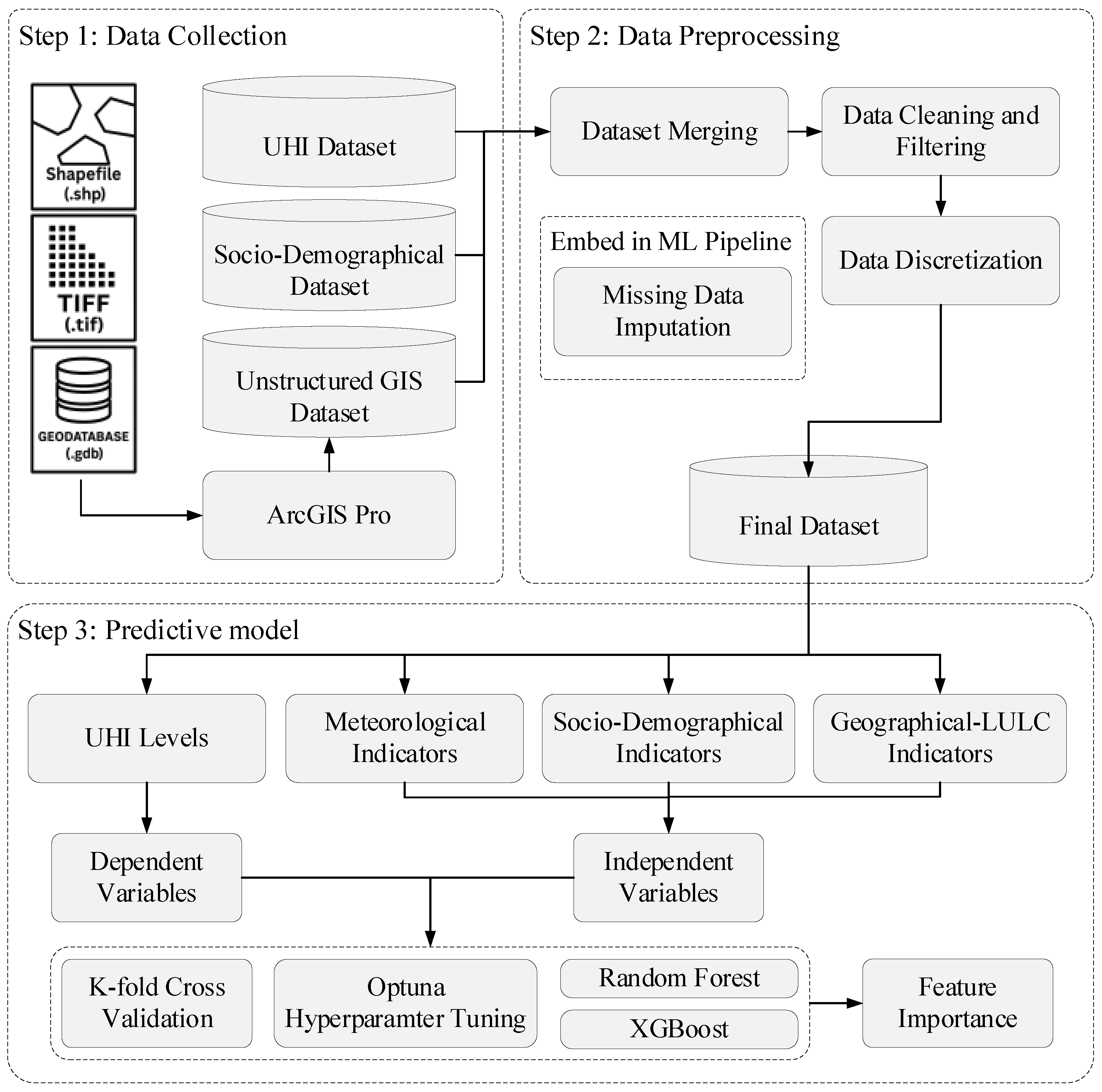
3. Materials and Methods

The methodological framework of this study was developed in four steps. First, UHI intensity data and influential indicator data were collected and integrated into a single dataset. Second, preprocessing functions were applied to prepare the data for training. Third, the machine learning models were trained to predict UHI intensity. Lastly, the importance of the input features was determined. Figure 1 presents the details of these steps. This study focused on urbanized areas in the Midwestern United States, encompassing twelve states: Illinois, Indiana, Iowa, Kansas, Michigan, Minnesota, Missouri, Nebraska, North Dakota, Ohio, South Dakota, and Wisconsin. This region offers a compelling case study due to its increasing vulnerability to climate extremes, diverse patterns of land use and urban development, and its relative underrepresentation in existing UHI research [35,36].

3.1. Data Collection

To predict UHI intensity, influential indicators were initially identified based on the existing literature. For temporal consistency, all datasets were standardized to represent conditions for or around the year 2020. The final unit of analysis for all features was the census tract, though the native spatial resolution of the source data varied. We selected indicators for which data were available for our study area and included additional relevant features. The required data were collected from multiple sources in two formats: structured (tabular data) and unstructured (shapefiles and TIFF files). The UHI and socio-demographical dataset were available at the census tract level while some geographical variables of unstructured dataset were derived from 30 m resolution raster files and subsequently aggregated. In total, 69 factors were obtained; due to this large number, they were grouped, and these groups are listed in

Table 4. Category and data source of group factors.

Category	Group Name	Abbreviation	Number of Factors	Source
Meteorological factors	Mean Annual Temperature	AT	1	Global Climate Monitor, 2020 [61]
	Mean Annual Rainfall	AR	1	Global Climate Monitor, 2020 [61]
Geographical–LULC factors	Digital Elevation Model (Urban and Rural)	DEM	2	Chakraborty et al., 2020 [62]
	Urban and Rural Digital Elevation Model Difference	DelDEM	1	Chakraborty et al., 2020 [62]
	NDVI (Urban and Rural) (Annual, Summer and Winter)	NDVI	6	Chakraborty et al., 2020 [62]
	Urban and Rural NDVI Difference (Annual, Summer and Winter)	DelNDVI	3	Chakraborty et al., 2020 [62]
	Tree Canopy	TC	1	Multi-Resolution Land Characteristics Consortium (MLRC), 2020 [63]
	Imperviousness	IMP	1	Multi-Resolution Land Characteristics Consortium (MLRC), 2020 [64]
	Building Area	BA	1	Heris et al. 2020 [65]
	Building Height	BH	1	Department of the Interior [66]
	Distance to Coast	DTC	1	Natural Earth. 2023 [67]
	Land Area	LA	1	U.S. Census Bureau [68]
Socio-demographical factors	Population	P	3	U.S. Census Bureau [69]
	Population Density	PD	1	U.S. Census Bureau [69]
	Age	AG	7	U.S. Census Bureau [69]
	Gender	G	2	U.S. Census Bureau [69]
	Ethnicity	ET	8	U.S. Census Bureau [69]
	Education level	EL	3	U.S. Census Bureau [69]
	Health Insurance Coverage	HIC	3	U.S. Census Bureau [69]
	Employment Status	ES	2	U.S. Census Bureau [69]
	Household Income	HI	2	U.S. Census Bureau [69]
	Housing Price	HP	2	U.S. Census Bureau [69]
	Housing Units	HU	7	U.S. Census Bureau [69]
	Access to Computers and the Internet	ACI	7	U.S. Census Bureau [69]
	Number of Persons per Household	NPH	2	U.S. Census Bureau [69]

. For example, the Age group includes seven factors, each representing the percentage of people within a specific age range.

3.1.1. UHI Dataset

The primary data source in this paper was the U.S. surface urban heat island database published by Chakraborty et al. [62]. This database contains data for all census tracts within U.S. urbanized areas. In addition to UHI intensity values, it includes other factors such as the Digital Elevation Model (DEM), Normalized Difference Vegetation Index (NDVI), and subsidiary factors derived from primary indicators (e.g., by subtracting rural from urban values). In total, 12 factors were extracted from this dataset.

3.1.2. Socio-Demographical Dataset

Socio-demographic data were collected from the planning database available on the U.S. Census Bureau website [68]. This database contains demographic, socio-economic, and housing factors based on the decennial census (CEN) and the American Community Survey (ACS) 5-year estimates. In this study, for factors available from both CEN and ACS, the CEN version was selected due to its higher reported accuracy. The dataset includes factors such as population, age, ethnicity, education level, health insurance coverage, employment status, household income, housing price, number of housing units, access to computers and the internet, and the number of persons per household. In addition to these, population density (PD), a factor considered in previous studies, was also included. This factor is calculated by dividing the population by the land area. Including PD, a total of 50 related factors were extracted from this dataset.

3.1.3. Unstructured Dataset

Other features, including mean annual temperature (AT), mean annual rainfall (AR), distance to coast (DTC), tree canopy (TC), building area (BA), average building height (BH), and imperviousness (IMP), had data types of either shapefile or TIFF files. ArcGIS Pro (version 3.4.2) was utilized to extract data from these files. Initially, the census tracts layer for the twelve states, collected from the U.S. Census Bureau [69], was imported as a shapefile into the software. These were then integrated into a single layer representing Midwestern census tracts. To ensure consistent measurement units, this layer’s coordinate reference system (CRS) was projected to USA Contiguous Albers Equal Area Conic. The following process was undertaken for the factors:

• DTC: To calculate DTC, the shapefile of the Earth’s coastline was first imported into the software. Then, geometric centroids of the census tracts were derived based on their polygonal boundaries. Lastly, using the Proximity tool, the closest distance from the centroids to the coastline was calculated.
• IMP and TC: These factors are in TIFF format. After importing them into the software, the Zonal Statistics tool was used to calculate the mean value of their pixels intersecting with the census tracts.
• BA: This factor is in TIFF form and each state had a separate file. After importing the state files, the Zonal Statistics tool was applied to each to calculate the sum of pixel values intersecting the census tracts. These outputs were then merged and added to the Midwestern census tracts layer.
• AR and AT: These factors were in tabular format, containing longitude and latitude of data points. The spatial resolution of these data was coarser than that of census tracts. To address this difference in spatial resolution, we employed the Spatial Join tool within ArcGIS. For the join operation, the CLOSEST match option was selected. This method identifies the single closest AR or AT data point to each census tract polygon and assigns its value accordingly. This technique is functionally a nearest neighbor assignment, chosen for its directness in linking each census tract to the most proximate available measurement.
• BH: These data were obtained in (GDB) format. Like other factors, the data were imported into the software. These data are at the block group level, which is a finer resolution than census tracts. Therefore, the Spatial Join tool was first utilized to assign values from intersecting block groups to each census tract. Second, the Summary Statistics tool was used to average these values for each census tract.

After extracting each factor their data were added to the Midwest layer as new column using Join Field tool. At the end, the Midwest layer was exported to the csv file as a table including census tract GEOID and factors columns.

3.2. Data Preprocessing

3.2.1. Dataset Merging

A unified dataset for analysis was created by merging the geographical/LULC and socio-demographic data using the census tract GEOID as the common identifier. This was achieved in two main stages. First, all geographical and LULC features, which existed in diverse spatial formats (as detailed in Section 3.1.3), were processed and aggregated to the census tract level. This crucial step standardized all spatial factors into a single attribute table where each row corresponded to a unique census tract. Second, this spatially derived table and the separate socio-demographic dataset were both joined to the base UHI dataset in a final tabular merge. This resulted in the comprehensive dataset of 11,972 rows used for the analysis.

3.2.2. Data Cleaning and Filtering

In this step, rows with null values for the UHI factor (12 rows) were dropped. Consistent with the study’s scope of investigating factors causing increased urban temperatures relative to rural areas, UHI values below −1 (representing an urban cooling effect) were filtered out. After cleaning and filtering, 10,795 rows remained in the dataset.

3.2.3. Data Discretization

The classification of UHI intensity into discrete levels was based on established thresholds from previous research to ensure comparability and validity. Specifically, we adapted the classification scheme used by studies such as Assaf et al. (2023) [31] and Lin et al. (2021) [70], which define four primary UHI levels: non-existent/negligible (e.g., −1 to 1 °C), slight (1 to 3 °C), moderate (3 to 5 °C), and strong (>5 °C).

For this study, a key consideration was maintaining a balanced distribution of data across categories for our analysis. The initial distribution showed fewer instances in the moderate and strong categories. Therefore, to avoid potential biases from an imbalanced dataset, we merged these two upper tiers. This resulted in the three UHI levels used in our analysis: Negligible (−1 ≤ UHI < 1), Low (1 ≤ UHI < 3), and High (UHI ≥ 3). The ranges and distribution for these final levels are shown in

Table 5. UHI severity classification and distribution.

UHI Level	Range	Distribution (%)
Negligible	−1 ≤ UHI < 1	31.9%
Low	1 ≤ UHI < 3	39.4%
High	3 ≤ UHI	28.7%

.

3.2.4. Missing Data Handling and Imputation

Prior to model development, the nature of missing data within the dataset was investigated to ensure the selection of an appropriate handling strategy. Analysis of missingness patterns using a correlation heatmap revealed a structured, non-random distribution. High correlations in missingness were observed across blocks of features, indicating that the data are not Missing Completely at Random (MCAR). This pattern is characteristic of a Missing at Random (MAR) mechanism, where the propensity for a value to be missing is correlated with other observed variables in the dataset [71].

Given the MAR nature of the data, a multivariate imputation approach was selected to avoid the bias associated with simpler methods like mean imputation. Specifically, K-Nearest Neighbors (KNN) imputation was employed for the Random Forest model. This technique estimates a missing value by calculating the weighted average of the values from its k most similar neighbors, where similarity is determined based on the other available features. This approach leverages the underlying structure of the data to produce more reliable estimates for missing entries.

To prevent data leakage and avoid affecting the test data, this imputation process was embedded within the ML model pipeline [72,73]. The imputer was fitted exclusively on the training data and then used to transform both the training and test datasets. This imputation was applied only to the Random Forest model, as the XGBoost algorithm includes a native, sparsity-aware methodology for handling missing values [74].

3.3. Predictive Model and Feature Importance

In this paper, the target variable is the UHI level, represented as a categorical value, making classification models the appropriate choice. Ensemble learning models have been widely used in recent years for both regression and classification problems [34]. This study utilizes Random Forest, a bagging method, and XGBoost, a boosting method, both of which are ensemble learning techniques. To assess performance, K-Fold Cross-Validation, a widely used machine learning technique, was employed [75]. This method enhances model generalizability as training is performed across various subsets of the dataset, rather than on a single, fixed data partition. A K-value of three was selected for the hyperparameter optimization phase to ensure computational efficiency across numerous trials. For the final model evaluation, K was increased to five to provide a more robust and accurate assessment of performance with the optimal hyperparameters. In this method, the dataset is divided into K folds (parts). In each iteration, one-fold is held out as the validation set, while the model is trained on the remaining K-1 folds.

To evaluate the predictive performance of the models, this study employed standard statistical metrics commonly used in classification analysis [76,77,78]. Four metrics were used: accuracy, precision, recall, and F1-score (Equations (1)–(4)).

$$Accuracy={\displaystyle \frac{TP+TN}{TP+FP+TN+FN}}$$

(1)

$$Precision={\displaystyle \frac{TP}{TP+FP}}$$

(2)

$$Recall={\displaystyle \frac{TP}{TP+FN}}$$

(3)

$$F1={\displaystyle \frac{2\times (Precision\times Recall)}{Precision+Recall}}$$

(4)

where TP, TN, FP, and FN are true positive, true negative, false positive, and false negative, respectively. To enhance model performance, machine learning models require optimization by identifying the hyperparameters that yield the best results. In this study, Optuna [79] was used for automatic hyperparameter optimization. Optuna efficiently searches for optimal hyperparameter values through an iterative process, aiming to maximize model performance. The search spaces for the hyperparameters (detailed in

Table A1. Hyperparameter search spaces for model optimization.

Model	Hyperparameter	Range/Values	Distribution/Type
Random Forest	n_estimators	[100, 300]	Integer
	max_depth	[10, 30]	Integer (Logarithmic)
	min_samples_split	[2, 10]	Integer
	min_samples_leaf	[1, 10]	Integer
	max_features	[‘sqrt’, ‘log2’, None]	Categorical
	class_weight	[‘balanced’, ‘balanced_subsample’, None]	Categorical
XGBoost	n_estimators	[50, 500]	Integer (Step: 50)
	max_depth	[3, 15]	Integer
	learning_rate	[0.001, 0.3]	Float (Logarithmic)
	subsample	[0.5, 1.0]	Float
	colsample_bytree	[0.5, 1.0]	Float
	gamma	[0, 5]	Float
	min_child_weight	[1, 20]	Integer
	reg_alpha (L1)	[1 × 10−8, 1.0]	Float (Logarithmic)
	reg_lambda (L2)	[1 × 10−8, 1.0]	Float (Logarithmic)

) were defined based on established machine learning practices to balance a comprehensive search with computational feasibility. Optuna employs a Bayesian optimization algorithm, specifically the Tree-structured Parzen Estimator (TPE), to identify promising hyperparameter value ranges. Finally, we determined feature importances using the models’ built-in functions. For the Random Forest classifier, this refers to the mean decrease in impurity (MDI), commonly known as Gini importance. For the XGBoost classifier, we used the default weight metric, which counts the number of times a feature is used to make a split across all trees.

4. Results

Figure 2 displays the spatial distribution of data points across U.S. Midwestern on an OpenStreetMap base layer, showing state borders.

As observed in Figure 2, the number of data points varies significantly among states. Figure 3 shows the percentage distribution of data points across these Midwestern states. Dominant states include Illinois (IL), Ohio (OH), and Michigan (MI), reflecting the presence of more urbanized and high-density areas in these states. Conversely, states such as South Dakota (SD), Nebraska (NE), and North Dakota (ND) contribute a smaller percentage of data points, indicating less urbanization and lower population density.

Figure 4 presents the average UHI intensity per state. Nebraska (NE) and Kansas (KS) exhibit the lowest average UHI intensities (approximately 1 °C), potentially reflecting less urban density or more extensive vegetation cover within their census tracts. In contrast, Wisconsin (WI), Michigan (MI), and Illinois (IL) display the highest average UHI intensities (approximately 2.3 °C), likely indicative of denser urbanization and reduced green cover. This visualization emphasizes the regional disparities in UHI effects across Midwestern urbanized zones.

Figure 5 illustrates the distribution of positive annual daytime UHI values. Peak density is observed in the 0 to 3 °C range, indicating that a large proportion of census tracts experience low to moderate UHI intensity. The long tail extending toward higher values (approximately 4 to 7 °C) suggests the presence of urban areas with significantly high UHI effects.

The optimal hyperparameter values for the Random Forest and XGBoost models, obtained using Optuna, are presented in

Table 6. Optimal hyperparameters for Random Forest and XGBoost models.

Random Forrest		XGBoost
Parameter	Optimum Value	Parameter	Optimum Value
n_estimators	151	n_estimators	150
max_depth	24	max_depth	9
min_samples_split	7	learning_rate	0.073
min_samples_leaf	2	subsample	0.857
max_features	None	colsample_bytree	0.666
class_weight	None	gamma	0.463
imputer_n_neighbors	12	min_child_weight	8
		reg_alpha	3.31 × 10−3
		reg_lambda	4.67 × 10−6

.

Table 7. Performance metrics for Random Forest and XGBoost models.

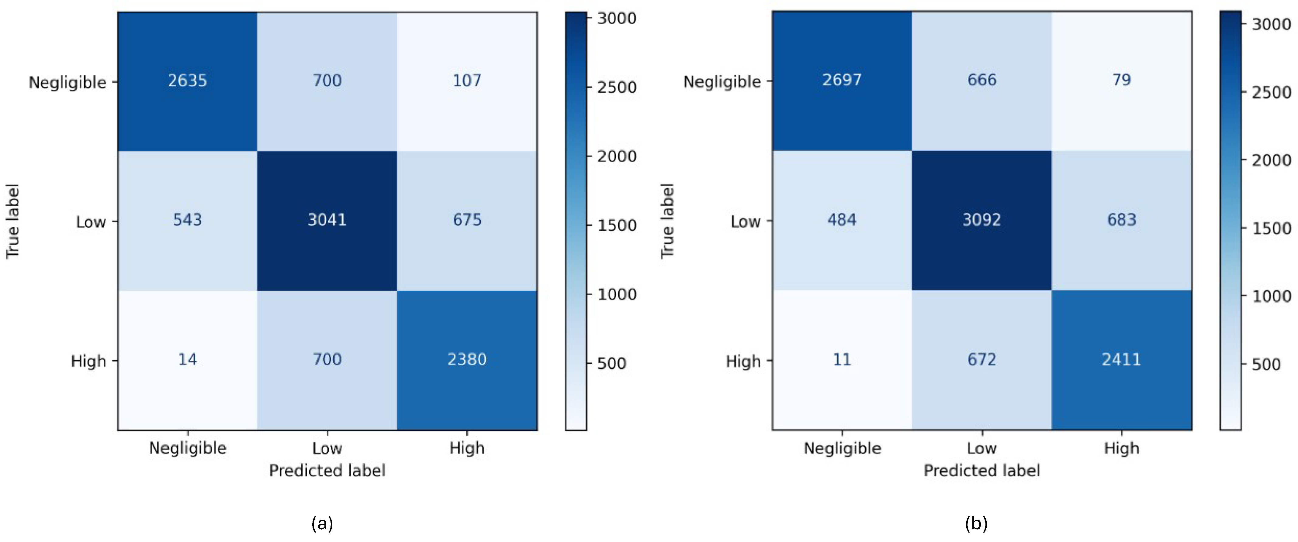
Model	Class	Precision	Recall	F1-Score	Sample Count
Random Forrest	Negligible	0.83	0.77	0.79	3442
	Low	0.68	0.71	0.7	4259
	High	0.75	0.77	0.76	3094
	Accuracy	-	-	0.75	10,795
	Macro avg	0.75	0.75	0.75	10,795
	Weighted avg	0.75	0.75	0.75	10,795
	Cohen’s Kappa *	-	-	0.62	-
	ROC-AUC *	-	-	0.9	-
XGBoost	Negligible	0.84	0.78	0.81	3442
	Low	0.7	0.73	0.71	4259
	High	0.76	0.78	0.77	3094
	Accuracy	-	-	0.76	10,795
	Macro avg	0.77	0.76	0.76	10,795
	Weighted avg	0.76	0.76	0.76	10,795
	Cohen’s Kappa *	-	-	0.64	-
	ROC-AUC *	-	-	0.91	-

* Cohen’s Kappa and ROC-AUC scores represent the average performance across all cross-validation folds.

presents the performance metrics, and Figure 6 displays the confusion matrices for both models. While there was not a substantial difference in the performance of the two models, XGBoost slightly outperformed Random Forest, achieving higher macro and weighted F1-scores (0.76 vs. 0.75, respectively). This strong performance is further supported by the high ROC-AUC scores (0.91 for XGBoost and 0.90 for Random Forest), indicating excellent discriminatory power between classes. Additionally, Cohen’s Kappa scores of 0.64 (XGBoost) and 0.62 (Random Forest) confirm that the models achieve substantial agreement, performing significantly better than random chance. For the negligible UHI class, both models demonstrated strong precision and recall. However, performance for the low UHI class was notably lower (F1-scores ≈ 0.7), indicating challenges in distinguishing this class from others, particularly the high UHI impact level. The confusion matrices further highlight this trend, with both models achieving high true positive rates for the negligible class. Although the class distribution is relatively balanced (31.9%, 39.4%, and 28.7% for negligible, low, and high, respectively), the misclassification pattern suggests overlapping feature distributions between the low and adjacent classes. These overlaps may indicate that the current features do not fully capture the transitional characteristics between moderate and extreme UHI zones. Enhancing the model with more discriminative features or applying class-specific tuning could improve performance. These results suggest that while both models effectively identify areas with negligible UHI effects, further investigation into techniques such as data balancing or feature engineering [80] could enhance the classification of higher UHI impact levels.

The feature importance plot (Figure 7) illustrates the relative contributions of meteorological, geographical/Land Use Land Cover (LULC), and socio-demographic factors to Urban Heat Island (UHI) prediction. The top 20 features from both models are presented in this plot. Both models highlight key LULC features, such as DelNDVI_summer and IMP (Imperviousness), as major contributors. Socio-demographic factors generally exhibit a moderate influence, while meteorological factors contribute comparatively less to the predictions.

To elucidate the contributions of individual features to the model’s predictions, a SHAP analysis was performed on the optimized XGBoost classifier (Figure 8). For the high UHI class, a low DelNDVI_summer value—indicating a large urban vegetation deficit—exerts the strongest positive influence on the model output, followed by high values for Imperviousness and Population Density. For the negligible UHI class, the effects of these top features are predictably inverted. The analysis also reveals that lower values for Building Height (BH) are a significant positive contributor, increasing the likelihood of a negligible UHI prediction.

5. Discussion

In this paper, we implemented classification models to predict UHI levels across census tracts of Midwestern urbanized areas. Two models, Random Forest and XGBoost, were utilized to compare predictive performance and identify common important features. The performance of both models was similar, with XGBoost yielding slightly better results. The distribution of data points across the three classes of the target variable was relatively balanced; therefore, resampling techniques such as undersampling (which can lead to a loss of useful data) were not deemed necessary. Hyperparameter optimization was implemented for both models to enhance their performance on the dataset. Although the classification results were not perfect and some misclassification occurred, the average accuracy achieved was 0.76, suggesting that the selected features are indeed influential in UHI formation. However, it is likely that incorporating additional relevant features could further enhance UHI prediction accuracy.

The most important feature identified by both models was DelNDVI_summer. This feature represents the difference in the Normalized Difference Vegetation Index (NDVI) within an urban census tract compared to its surrounding rural reference area during the summer season. The SHAP analysis provides a more nuanced interpretation, revealing that the magnitude of this vegetation deficit is the primary driver of high UHI severity. Its prominence strongly indicates that the degree of urbanization, specifically the reduction in urban vegetation relative to rural areas, significantly contributes to increased urban temperatures. Two other features with high-ranking importance common to both models were LAND_AREA and IMP (Imperviousness). The significance of IMP demonstrates the substantial impact of impervious surfaces—such as concrete, pavements, and roofs—on the UHI effect. These surfaces typically reduce natural cooling by inhibiting evapotranspiration. Furthermore, many impervious materials absorb more solar radiation (due to lower albedo) and store larger amounts of heat compared to natural landscapes, subsequently releasing this stored heat and contributing to higher urban temperatures.

Demographic factors also emerged as notably important. In the feature importance rankings for both models, pct_RURAL_POP, pct_URBAN_POP, and PD were all among the top six most influential variables. These features, respectively, represent the percentage of people in areas with low and high housing density, and overall population density. Their collective importance underscores the impact of population density and urban congestion on heat generation, which potentially results from increased human activity and energy consumption in densely populated areas.

Tree Canopy (TC) is also a common feature within the top 20 for both models, and several other important variables are related to the Normalized Difference Vegetation Index (NDVI); collectively, these underscore the significance of vegetation in urbanized areas. The SHAP analysis further revealed that higher Building Height (BH) was a predictor for the high UHI class, likely due to its contribution to the urban canyon effect, which traps heat and reduces airflow. Meteorological variables, including average annual temperature and rainfall, also appeared among the top features, although their overall importance ranking was generally lower than that of LULC and socio-demographic factors. Furthermore, from a mitigation perspective, it is important to note that these weather variables are not directly controllable and thus cannot be altered to mitigate the UHI effect, unlike factors related to urban planning and green infrastructure, which reinforces their critical importance for climate-adaptive design.

This study offers reliable insights into the most effective factors contributing to the UHI effect, based on an analysis of over ten thousand census tracts. Sixty-nine features across diverse categories were considered, from which the most influential ones were identified. These findings can inform strategies to mitigate the UHI effect. While some factors, such as population density, are largely established and challenging to alter existing developed areas, their careful consideration is crucial in the planning and development of new urban regions. In contrast, other critical factors, particularly those related to vegetation cover (as indicated by metrics like the NDVI), are more amenable to modification even in densely built environments. Interventions can include creating parks and green spaces; furthermore, where ground-level space is limited, implementing green roofs presents a viable and effective option for UHI mitigation.

Our findings, emphasizing the importance of vegetation, align well with the green infrastructure strategies common in Midwestern cities. These approaches, which focus on restoring evaporative cooling, differ from those in arid regions like the Southwestern U.S., where mitigation often prioritizes increasing surface albedo with reflective ‘cool’ materials. This highlights that UHI drivers are highly region-specific, reinforcing the need for localized studies like ours to inform effective and context-appropriate urban planning.

Finally, we must acknowledge a methodological limitation related to the spatial nature of the data. The proximity of census tracts can result in spatial autocorrelation, which may inflate performance metrics when using standard cross-validation. To investigate this, we conducted a sensitivity analysis with a spatially blocked cross-validation that prevents this information leakage. This test yielded a more conservative accuracy of 0.70. While this confirms the general robustness of our findings, it underscores that future work in this area could benefit from employing explicit spatial regression models to more formally account for these geographic effects.

6. Conclusions

This paper demonstrated the effectiveness of ensemble learning techniques for predicting UHI levels and identifying key contributing factors across Midwestern urbanized areas. Two robust classification models, Random Forest and XGBoost, were employed. Although XGBoost yielded slightly better performance, the use of both models facilitated the verification of results and reinforced the overall findings. The top twenty most important features from both models were identified. Notably, while the majority of input features belonged to the socio-demographic category, geographical and land use/land cover (LULC) features emerged as more impactful. Many of these, including NDVI-related features, Imperviousness (IMP), and Tree Canopy (TC), pinpoint the significant role of vegetation and green spaces in urbanized areas. Key socio-demographic features such as pct_RURAL_POP, pct_URBAN_POP, and Population Density (PD) were also ranked among the top five most influential factors.

These findings can inform urban planners and policymakers in developing and employing efficient strategies to mitigate the UHI effect. The insights can be applied to reduce UHI intensity in areas currently struggling with this issue and to guide preventative measures in developing urban regions. Increasing vegetation through the implementation of green roofs and the creation of green spaces, particularly in high-density areas, can considerably reduce the UHI effect. While such greening methods are effective, space constraints may limit their applicability in certain contexts. Therefore, developing and utilizing sustainable construction materials, such as concrete and pavements designed to absorb less heat, can also contribute significantly to UHI reduction.

In this paper, we investigated all urbanized census tracts of the Midwestern United States, incorporating sixty-nine distinct features. Two robust machine learning models were employed, and an optimization algorithm was utilized for hyperparameter tuning. Despite these efforts, the classification models did not achieve perfect accuracy, with some instances being misclassified. A limitation of this study is that the selected features, while extensive, may not entirely encompass all drivers of UHI intensity, and the inclusion of additional relevant variables could potentially enhance model performance. Additionally, because the model is calibrated for the Midwest, its findings may not be directly transferable to regions with different climatic or urban contexts without further validation. Future research could expand upon the Explainable AI (XAI) analysis [80] presented here—for instance, by examining complex feature interactions—and investigate a broader range of factors impacting UHI, such as urban form metrics and temporal variables (e.g., inter-annual LST variation). Moreover, further investigation into the efficacy and context-specific application of diverse sustainable UHI mitigation strategies would be beneficial. Finally, future work should aim to directly integrate this predictive modeling framework into policy simulation tools to allow planners to quantitatively assess the potential impact of specific interventions, thereby explicitly bridging the gap between technical analysis and actionable policy.

References

- Du, H.; Wang, D.; Wang, Y.; Zhao, X.; Qin, F.; Jiang, H.; Cai, Y. Influences of Land Cover Types, Meteorological Conditions, Anthropogenic Heat and Urban Area on Surface Urban Heat Island in the Yangtze River Delta Urban Agglomeration. Sci. Total Environ. 2016, 571, 461–470. [Google Scholar] [CrossRef] [PubMed]
- Erfani, A.; Tavakolan, M. Risk Evaluation Model of Wind Energy Investment Projects Using Modified Fuzzy Group Decision-Making and Monte Carlo Simulation. Arthaniti J. Econ. Theory Pract. 2023, 22, 7–33. [Google Scholar] [CrossRef]
- Yang, K.; Zhang, J.; Cui, D.; Ma, Y.; Ye, Y.; He, X.; Zhang, Y. Multi-Scale Study of the Synergy Between Human Activities and Climate Change on Urban Heat Islands in China. Sustain. Cities Soc. 2025, 125, 106341. [Google Scholar] [CrossRef]
- Li, D.; Hu, X.; Rollo, J.; Luther, M.; Lu, M.; Liu, C. Spatial Cluster Characteristics of Land Surface Temperatures. Sustainability 2025, 17, 2653. [Google Scholar] [CrossRef]
- Li, H.; Meier, F.; Lee, X.; Chakraborty, T.; Liu, J.; Schaap, M.; Sodoudi, S. Interaction Between Urban Heat Island and Urban Pollution Island During Summer in Berlin. Sci. Total Environ. 2018, 636, 818–828. [Google Scholar] [CrossRef]
- Piracha, A.; Chaudhary, M.T. Urban Air Pollution, Urban Heat Island and Human Health: A Review of the Literature. Sustainability 2022, 14, 9234. [Google Scholar] [CrossRef]
- Aboelata, A. Vegetation in Different Street Orientations of Aspect Ratio (H/W 1:1) to Mitigate UHI and Reduce Buildings’ Energy in Arid Climate. Build. Environ. 2020, 172, 106712. [Google Scholar] [CrossRef]
- Wang, S.Y.; Ou, H.Y.; Chen, P.C.; Lin, T.P. Implementing Policies to Mitigate Urban Heat Islands: Analyzing Urban Development Factors with an Innovative Machine Learning Approach. Urban Clim. 2024, 55, 101868. [Google Scholar] [CrossRef]
- Rizwan, A.M.; Dennis, L.Y. A Review on the Generation, Determination and Mitigation of Urban Heat Island. J. Environ. Sci. 2008, 20, 120–128. [Google Scholar] [CrossRef]
- U.S. Environmental Protection Agency. Climate Change Indicators: Heat Waves. Available online: https://www.epa.gov/climate-indicators/climate-change-indicators-heat-waves (accessed on 2 May 2025).
- Bao, Y.; Li, Y.; Gu, J.; Shen, C.; Zhang, Y.; Deng, X.; Ran, J. Urban Heat Island Impacts on Mental Health in Middle-Aged and Older Adults. Environ. Int. 2025, 199, 109470. [Google Scholar] [CrossRef]
- He, B.J.; Wang, J.; Liu, H.; Ulpiani, G. Localized Synergies Between Heat Waves and Urban Heat Islands: Implications on Human Thermal Comfort and Urban Heat Management. Environ. Res. 2021, 193, 110584. [Google Scholar] [CrossRef]
- Heaviside, C.; Macintyre, H.; Vardoulakis, S. The Urban Heat Island: Implications for Health in a Changing Environment. Curr. Environ. Health Rep. 2017, 4, 296–305. [Google Scholar] [CrossRef] [PubMed]
- Yang, J.; Siri, J.G.; Remais, J.V.; Cheng, Q.; Zhang, H.; Chan, K.K.; Gong, P. The Tsinghua–Lancet Commission on Healthy Cities in China: Unlocking the Power of Cities for a Healthy China. Lancet 2018, 391, 2140–2184. [Google Scholar] [CrossRef] [PubMed]
- Foroutan, E.; Hu, T.; Li, Z. Revealing Key Factors of Heat-Related Illnesses Using Geospatial Explainable AI Model: A Case Study in Texas, USA. Sustain. Cities Soc. 2025, 122, 106243. [Google Scholar] [CrossRef]
- Assaf, G.; Hu, X.; Assaad, R.H. Mining and Modeling the Direct and Indirect Causalities Among Factors Affecting the Urban Heat Island Severity Using Structural Machine Learned Bayesian Networks. Urban Clim. 2023, 49, 101570. [Google Scholar] [CrossRef]
- Han, D.; Zhang, T.; Qin, Y.; Tan, Y.; Liu, J. A Comparative Review on the Mitigation Strategies of Urban Heat Island (UHI): A Pathway for Sustainable Urban Development. Clim. Dev. 2023, 15, 379–403. [Google Scholar] [CrossRef]
- Aslani, A.; Sereshti, M.; Sharifi, A. Urban Heat Island Mitigation in Tehran: District-Based Mapping and Analysis of Key Drivers. Sustain. Cities Soc. 2025, 125, 106338. [Google Scholar] [CrossRef]
- Cai, P.; Li, R.; Guo, J.; Xiao, Z.; Fu, H.; Guo, T.; Song, X. Multi-Scale Spatiotemporal Patterns of Urban Climate Effects and Their Driving Factors Across China. Urban Clim. 2025, 60, 102350. [Google Scholar] [CrossRef]
- Petrou, I.; Kassomenos, P. Estimating the Importance of Environmental Factors Influencing the Urban Heat Island for Urban Areas in Greece: A Machine Learning Approach. J. Environ. Manag. 2024, 368, 122255. [Google Scholar] [CrossRef]
- Xu, J.; Jin, Y.; Ling, Y.; Sun, Y.; Wang, Y. Exploring the Seasonal Impacts of Morphological Spatial Pattern of Green Spaces on the Urban Heat Island. Sustain. Cities Soc. 2025, 125, 106352. [Google Scholar] [CrossRef]
- Xu, D.; Wang, Y.; Zhou, D.; Wang, Y.; Zhang, Q.; Yang, Y. Influences of Urban Spatial Factors on Surface Urban Heat Island Effect and Its Spatial Heterogeneity: A Case Study of Xi’an. Build. Environ. 2024, 248, 111072. [Google Scholar] [CrossRef]
- Mathew, A.; Arunab, K.S.; Sharma, A.K. Revealing the Urban Heat Island: Investigating Spatiotemporal Surface Temperature Dynamics, Modeling, and Interactions with Controllable and Non-Controllable Factors. Remote Sens. Appl. Soc. Environ. 2024, 35, 101219. [Google Scholar] [CrossRef]
- Ghorbany, S.; Hu, M.; Yao, S.; Wang, C. Towards a Sustainable Urban Future: A Comprehensive Review of Urban Heat Island Research Technologies and Machine Learning Approaches. Sustainability 2024, 16, 4609. [Google Scholar] [CrossRef]
- Adilkhanova, I.; Ngarambe, J.; Yun, G.Y. Recent Advances in Black Box and White-Box Models for Urban Heat Island Prediction: Implications of Fusing the Two Methods. Renew. Sustain. Energy Rev. 2022, 165, 112520. [Google Scholar] [CrossRef]
- Mansouri, A.; Naghdi, M.; Erfani, A. Machine Learning for Leadership in Energy and Environmental Design Credit Targeting: Project Attributes and Climate Analysis Toward Sustainability. Sustainability 2025, 17, 2521. [Google Scholar] [CrossRef]
- Koc, M.; Acar, A. Investigation of Urban Climates and Built Environment Relations by Using Machine Learning. Urban Clim. 2021, 37, 100820. [Google Scholar] [CrossRef]
- Erfani, A.; Cui, Q. Predictive Risk Modeling for Major Transportation Projects Using Historical Data. Autom. Constr. 2022, 139, 104301. [Google Scholar] [CrossRef]
- Oh, J.W.; Ngarambe, J.; Duhirwe, P.N.; Yun, G.Y.; Santamouris, M. Using Deep-Learning to Forecast the Magnitude and Characteristics of Urban Heat Island in Seoul, Korea. Sci. Rep. 2020, 10, 3559. [Google Scholar] [CrossRef]
- Tanoori, G.; Soltani, A.; Modiri, A. Machine Learning for Urban Heat Island (UHI) Analysis: Predicting Land Surface Temperature (LST) in Urban Environments. Urban Clim. 2024, 55, 101962. [Google Scholar] [CrossRef]
- Assaf, G.; Hu, X.; Assaad, R.H. Predicting Urban Heat Island Severity on the Census-Tract Level Using Bayesian Networks. Sustain. Cities Soc. 2023, 97, 104756. [Google Scholar] [CrossRef]
- Tehrani, A.A.; Veisi, O.; Delavar, Y.; Bahrami, S.; Sobhaninia, S.; Mehan, A. Predicting Urban Heat Island in European Cities: A Comparative Study of GRU, DNN, and ANN Models Using Urban Morphological Variables. Urban Clim. 2024, 56, 102061. [Google Scholar] [CrossRef]
- Hoang, N.D.; Nguyen, Q.L. Geospatial Analysis and Machine Learning Framework for Urban Heat Island Intensity Prediction: Natural Gradient Boosting and Deep Neural Network Regressors with Multisource Remote Sensing Data. Sustainability 2025, 17, 4287. [Google Scholar] [CrossRef]
- Dong, X.; Yu, Z.; Cao, W.; Shi, Y.; Ma, Q. A Survey on Ensemble Learning. Front. Comput. Sci. 2020, 14, 241–258. [Google Scholar] [CrossRef]
- Lyu, F.; Wang, S.; Han, S.Y.; Catlett, C.; Wang, S. An Integrated CyberGIS and Machine Learning Framework for Fine-Scale Prediction of Urban Heat Island Using Satellite Remote Sensing and Urban Sensor Network Data. Urban Inform. 2022, 1, 6. [Google Scholar] [CrossRef]
- Hashemi, F.; Najafian, P.; Salahi, N.; Ghiasi, S.; Passe, U. The Impact of the Urban Heat Island and Future Climate on Urban Building Energy Use in a Midwestern US Neighborhood. Energies 2025, 18, 1474. [Google Scholar] [CrossRef]
- Kim, M.; Lee, K.; Cho, G.H. Temporal and Spatial Variability of Urban Heat Island by Geographical Location: A Case Study of Ulsan, Korea. Build. Environ. 2017, 126, 471–482. [Google Scholar] [CrossRef]
- Acosta, M.P.; Vahdatikhaki, F.; Santos, J.; Hammad, A.; Dorée, A.G. How to Bring UHI to the Urban Planning Table? A Data-Driven Modeling Approach. Sustain. Cities Soc. 2021, 71, 102948. [Google Scholar] [CrossRef]
- Singh, M.; Sharston, R.; Murtha, T. Critical Evaluation of the Spatiotemporal Behavior of UHI, Through Correlation Analyses Based on Multi-City Heterogeneous Dataset. Sustain. Cities Soc. 2024, 110, 105576. [Google Scholar] [CrossRef]
- Ngarambe, J.; Oh, J.W.; Su, M.A.; Santamouris, M.; Yun, G.Y. Influences of Wind Speed, Sky Conditions, Land Use and Land Cover Characteristics on the Magnitude of the Urban Heat Island in Seoul: An Exploratory Analysis. Sustain. Cities Soc. 2021, 71, 102953. [Google Scholar] [CrossRef]
- Zheng, Z.; Lin, X.; Chen, L.; Yan, C.; Sun, T. Effects of Urbanization and Topography on Thermal Comfort During a Heat Wave Event: A Case Study of Fuzhou, China. Sustain. Cities Soc. 2024, 102, 105233. [Google Scholar] [CrossRef]
- Hidalgo-García, D.; Arco-Díaz, J. Modeling the Surface Urban Heat Island (SUHI) to Study Its Relationship with Variations in the Thermal Field and with the Indices of Land Use in the Metropolitan Area of Granada (Spain). Sustain. Cities Soc. 2022, 87, 104166. [Google Scholar] [CrossRef]
- Xu, Z.; Rui, J. The Mitigating Effect of Green Space’s Spatial and Temporal Patterns on the Urban Heat Island in the Context of Urban Densification: A Case Study of Xi’an. Sustain. Cities Soc. 2024, 117, 105974. [Google Scholar] [CrossRef]
- Patel, S.; Indraganti, M.; Jawarneh, R.N. Land Surface Temperature Responses to Land Use Dynamics in Urban Areas of Doha, Qatar. Sustain. Cities Soc. 2024, 104, 105273. [Google Scholar] [CrossRef]
- Deilami, K.; Kamruzzaman, M.; Liu, Y. Urban Heat Island Effect: A Systematic Review of Spatio-Temporal Factors, Data, Methods, and Mitigation Measures. Int. J. Appl. Earth Obs. Geoinf. 2018, 67, 30–42. [Google Scholar] [CrossRef]
- Cetin, M.; Ozenen Kavlak, M.; Senyel Kurkcuoglu, M.A.; Bilge Ozturk, G.; Cabuk, S.N.; Cabuk, A. Determination of Land Surface Temperature and Urban Heat Island Effects with Remote Sensing Capabilities: The Case of Kayseri, Türkiye. Nat. Hazards 2024, 120, 5509–5536. [Google Scholar] [CrossRef]
- Yoo, S. Investigating Important Urban Characteristics in the Formation of Urban Heat Islands: A Machine Learning Approach. J. Big Data 2018, 5, 2. [Google Scholar] [CrossRef]
- Mehmood, M.S.; Rehman, A.; Sajjad, M.; Song, J.; Zafar, Z.; Shiyan, Z.; Yaochen, Q. Evaluating Land Use/Cover Change Associations with Urban Surface Temperature via Machine Learning and Spatial Modeling: Past Trends and Future Simulations in Dera Ghazi Khan, Pakistan. Front. Ecol. Evol. 2023, 11, 1115074. [Google Scholar] [CrossRef]
- Thambawita, T.K.C.N.; Munasinghe, D.S.; Yapa, L.K.K. Identification of Urban Heat Island Effect on Land Use Land Cover Changes. J. Geospat. Surv. 2023, 3, 43–53. [Google Scholar] [CrossRef]
- Ullah, S.; Khan, M.; Qiao, X. Evaluating the Impact of Urbanization Patterns on LST and UHI Effect in Afghanistan’s Cities: A Machine Learning Approach for Sustainable Urban Planning. Environ. Dev. Sustain. 2025, 1–42. [Google Scholar] [CrossRef]
- Hickey, P.J.; Erfani, A.; Cui, Q. Use of LinkedIn Data and Machine Learning to Analyze Gender Differences in Construction Career Paths. J. Manag. Eng. 2022, 38, 04022060. [Google Scholar] [CrossRef]
- Chaturvedi, V.; de Vries, W.T. Machine Learning Algorithms for Urban Land Use Planning: A Review. Urban Sci. 2021, 5, 68. [Google Scholar] [CrossRef]
- Casali, Y.; Aydin, N.Y.; Comes, T. Machine Learning for Spatial Analyses in Urban Areas: A Scoping Review. Sustain. Cities Soc. 2022, 85, 104050. [Google Scholar] [CrossRef]
- Equere, V.; Mirzaei, P.A.; Riffat, S.; Wang, Y. Integration of Topological Aspect of City Terrains to Predict the Spatial Distribution of Urban Heat Island Using GIS and ANN. Sustain. Cities Soc. 2021, 69, 102825. [Google Scholar] [CrossRef]
- O’Malley, C.; Piroozfar, P.; Farr, E.R.; Pomponi, F. Urban Heat Island (UHI) Mitigating Strategies: A Case-Based Comparative Analysis. Sustain. Cities Soc. 2015, 19, 222–235. [Google Scholar] [CrossRef]
- Mohammad, P.; Goswami, A.; Chauhan, S.; Nayak, S. Machine Learning Algorithm Based Prediction of Land Use Land Cover and Land Surface Temperature Changes to Characterize the Surface Urban Heat Island Phenomena Over Ahmedabad City, India. Urban Clim. 2022, 42, 101116. [Google Scholar] [CrossRef]
- Lin, J.; Qiu, S.; Tan, X.; Zhuang, Y. Measuring the Relationship Between Morphological Spatial Pattern of Green Space and Urban Heat Island Using Machine Learning Methods. Build. Environ. 2023, 228, 109910. [Google Scholar] [CrossRef]
- Guo, L.; Du, S.; Sun, W.; Fan, D.; Wu, Y. Multi-Scale Impact of Urban Building Function and 2D/3D Morphology on Urban Heat Island Effect: A Case Study in Shanghai, China. Energy Build. 2025, 338, 115719. [Google Scholar] [CrossRef]
- Hong, T.; Yim, S.H.; Heo, Y. Interpreting Complex Relationships Between Urban and Meteorological Factors and Street-Level Urban Heat Islands: Application of Random Forest and SHAP Method. Sustain. Cities Soc. 2025, 126, 106353. [Google Scholar] [CrossRef]
- Qiao, Z.; Jia, R.; Liu, J.; Gao, H.; Wei, Q. Remote Sensing-Based Analysis of Urban Heat Island Driving Factors: A Local Climate Zone Perspective. IEEE J. Sel. Top. Appl. Earth Obs. Remote Sens. 2024, 17, 17337. [Google Scholar] [CrossRef]
- Global Climate Monitor. Available online: https://www.globalclimatemonitor.org/ (accessed on 2 May 2025).
- Chakraborty, T.C.; Hsu, A.; Sheriff, G.; Manya, D. United States Surface Urban Heat Island Database. Mendeley Data 2020, V3. Available online: https://doi.org/10.17632/x9mv4krnm2.3 (accessed on 2 May 2025).
- Multi-Resolution Land Characteristics Consortium (MRLC). Dataset Type: Tree Canopy. Available online: https://www.mrlc.gov/data?f%5B0%5D=category%3ATree%20Canopy&f%5B1%5D=region%3Aconus&f%5B2%5D=year%3A2020 (accessed on 2 May 2025).
- Multi-Resolution Land Characteristics Consortium (MRLC). Dataset Type: Impervious Descriptor. Available online: https://www.mrlc.gov/data?f%5B0%5D=category%3AImpervious%20Descriptor&f%5B1%5D=region%3Aconus&f%5B2%5D=year%3A2020 (accessed on 2 May 2025).
- Heris, M.P.; Foks, N.; Bagstad, K.; Troy, A. A National Dataset of Rasterized Building Footprints for the U.S. U.S. Geological Survey Data Release 2020. Available online: https://doi.org/10.5066/P9J2Y1WG (accessed on 2 May 2025).
- Department of the Interior. U.S. National Categorical Mapping of Building Heights by Block Group from Shuttle Radar Topography Mission Data. Available online: https://catalog.data.gov/dataset/u-s-national-categorical-mapping-of-building-heights-by-block-group-from-shuttle-radar-top (accessed on 2 May 2025).
- Natural Earth. 1:10m Physical Vectors. 2023. Available online: https://www.naturalearthdata.com/downloads/10m-physical-vectors/ (accessed on 2 May 2025).
- U.S. Census Bureau. Planning Database. 2023. Available online: https://www.census.gov/topics/research/guidance/planning-databases.2023.html#list-tab-1219258324 (accessed on 2 May 2025).
- U.S. Census Bureau. TIGER/Line Shapefiles. 2023. Available online: https://www.census.gov/geographies/mapping-files/time-series/geo/tiger-line-file.2023.html#list-tab-790442341 (accessed on 2 May 2025).
- Lin, M.; Dong, J.; Jones, L.; Liu, J.; Lin, T.; Zuo, J.; Ye, H.; Zhang, G.; Zhou, T. Modeling Green Roofs’ Cooling Effect in High-Density Urban Areas Based on Law of Diminishing Marginal Utility of the Cooling Efficiency: A Case Study of Xiamen Island, China. J. Clean. Prod. 2021, 316, 128277. [Google Scholar] [CrossRef]
- Little, R.J.A.; Rubin, D.B. Statistical Analysis with Missing Data; John Wiley & Sons: Hoboken, NJ, USA, 2019; Available online: https://books.google.com/books?id=BemMDwAAQBAJ&lpg=PR11&ots=FCDO82DT1V&dq=Statistical%20Analysis%20with%20Missing%20Data%20(3rd%20ed.)&lr&pg=PR3#v=onepage&q=Statistical%20Analysis%20with%20Missing%20Data%20(3rd%20ed.)&f=false (accessed on 2 May 2025).
- Junninen, H.; Niska, H.; Tuppurainen, K.; Ruuskanen, J.; Kolehmainen, M. Methods for Imputation of Missing Values in Air Quality Data Sets. Atmos. Environ. 2004, 38, 2895–2907. [Google Scholar] [CrossRef]
- Adnan, T.; Erfani, A.; Cui, Q. Paving Equity: Unveiling Socioeconomic Patterns in Pavement Conditions Using Data Mining. J. Manag. Eng. 2025, 41, 04025041. [Google Scholar] [CrossRef]
- Chen, T.; Guestrin, C. XGBoost: A Scalable Tree Boosting System. In Proceedings of the 22nd ACM SIGKDD International Conference on Knowledge Discovery and Data Mining, San Francisco, CA, USA, 13–17 August 2016; pp. 785–794. [Google Scholar] [CrossRef]
- Wong, T.T.; Yeh, P.Y. Reliable Accuracy Estimates from k-Fold Cross Validation. IEEE Trans. Knowl. Data Eng. 2019, 32, 1586–1594. [Google Scholar] [CrossRef]
- Vujović, Ž. Classification Model Evaluation Metrics. Int. J. Adv. Comput. Sci. Appl. 2021, 12, 599–606. [Google Scholar] [CrossRef]
- Li, L.; Erfani, A.; Wang, Y.; Cui, Q. Anatomy into the Battle of Supporting or Opposing Reopening Amid the COVID-19 Pandemic on Twitter: A Temporal and Spatial Analysis. PLoS ONE 2021, 16, e0254359. [Google Scholar] [CrossRef]
- Erfani, A.; Cui, Q. Natural language processing application in construction domain: An integrative review and algorithms comparison. Comput. Civ. Eng. 2021, 2021, 26–33. Available online: https://ascelibrary.org/doi/abs/10.1061/9780784483893.004 (accessed on 2 May 2025).
- Akiba, T.; Sano, S.; Yanase, T.; Ohta, T.; Koyama, M. Optuna: A Next-Generation Hyperparameter Optimization Framework. In Proceedings of the 25th ACM SIGKDD International Conference on Knowledge Discovery & Data Mining, Anchorage, AK, USA, 4–8 August 2019; pp. 2623–2631. [Google Scholar] [CrossRef]
- Erfani, A.; Shayesteh, N.; Adnan, T. Data Augmented Explainable AI for Pavement Roughness Prediction. Autom. Constr. 2025, 176, 106307. [Google Scholar] [CrossRef]