Spatial Prediction of Soil Organic Carbon Based on a Multivariate Feature Set and Stacking Ensemble Algorithm: A Case Study of Wei-Ku Oasis in China

Abstract

Accurate estimation of soil organic carbon (SOC) content is crucial for assessing terrestrial ecosystem carbon stocks. Although traditional methods offer relatively high estimation accuracy, they are limited by poor timeliness and high costs. Combining measured data, remote sensing technology, and machine learning (ML) algorithms enables rapid, efficient, and accurate large-scale prediction. However, single ML models often face issues like high feature variable redundancy and weak generalization ability. Integrated models can effectively overcome these problems. This study focuses on the Weigan–Kuqa River oasis (Wei-Ku Oasis), a typical arid oasis in northwest China. It integrates Sentinel-2A multispectral imagery, a digital elevation model, ERA5 meteorological reanalysis data, soil attribute, and land use (LU) data to estimate SOC. The Boruta algorithm, Lasso regression, and its combination methods were used to screen feature variables, constructing a multidimensional feature space. Ensemble models like Random Forest (RF), Gradient Boosting Machine (GBM), and the Stacking model are built. Results show that the Stacking model, constructed by combining the screened variable sets, exhibited optimal prediction accuracy (test set R² = 0.61, RMSE = 2.17 g∙kg⁻¹, RPD = 1.61), which reduced the prediction error by 9% compared to single model prediction. Difference Vegetation Index (DVI), Bare Soil Evapotranspiration (BSE), and type of land use (TLU) have a substantial multidimensional synergistic influence on the spatial differentiation pattern of the SOC. The implementation of TLU has been demonstrated to exert a substantial influence on the model’s estimation performance, as evidenced by an augmentation of 24% in the R² of the test set. The integration of Boruta–Lasso combination screening and Stacking has been shown to facilitate the construction of a high-precision SOC content estimation model. This model has the capacity to provide technical support for precision fertilization in oasis regions in arid zones and the management of regional carbon sinks.

1. Introduction

Soil organic carbon (SOC) is a core element of terrestrial ecosystems and plays an important role in maintaining the ecological balance and climate stability of the Earth [1,2]. Accurate estimation of SOC content is imperative for a comprehensive understanding of the carbon cycle in terrestrial ecosystems and for the scientific evaluation of soil fertility. Although traditional SOC measurement methods are highly accurate, they suffer from poor timeliness and exhibit certain destructiveness. In contrast, advanced remote sensing spectroscopy technology offers a more effective alternative, enabling rapid, non-destructive, and large-scale monitoring [3]. In recent years, the development of remote sensing technology has provided a new solution path for SOC spatial prediction. By virtue of the advantages of remotely sensed data, such as large-scale accessibility and the ability to continuously acquire surface information [4], it provides an efficient and feasible technical means for the dynamic monitoring of SOC. Early remote sensing studies on SOC monitoring primarily relied on empirical statistical relationships between surface spectral reflectance and SOC content (e.g., single-band or spectral index modeling). However, surface spectral information is susceptible to interference from various factors such as vegetation cover, soil moisture, and surface roughness. This leads to limited model generalizability, resulting in the “same object with different spectra” phenomenon, and consequently low prediction accuracy [5]. The integration of digital soil mapping techniques into SOC monitoring has been facilitated by the advent of multi-source remote sensing data fusion and machine learning (ML) algorithms. In particular, the utilization of multivariate models founded upon ML algorithms has witnessed a marked increase in the context of SOC estimation studies [6,7,8]. In comparison with single ML models (e.g., linear regression, α), the ensemble learning algorithm has been shown to significantly improve the modeling performance of high-dimensional nonlinear data through the complementary advantages of heterogeneous base models. This provides a robust foundation for the in-depth exploration of soil properties and related ecological processes.

In the systematic study of key aspects such as feature variable screening and SOC modeling method optimization, scholars have found that there are significant differences in the contribution of each feature variable to the improvement of model prediction performance, and the estimation accuracy of different models is also quite different [9,10,11]. However, few studies have systematically evaluated the impact of various variables on modeling accuracy and analyzed their significance, particularly in complex agricultural ecosystems. For instance, Zhang et al. [12] demonstrated that the visible, short-wave infrared, and thermal infrared bands exhibited strong correlations with SOC content, based on Landsat 8 OLI data. In a similar vein, Xiao et al. [13] ensemble the raw spectral reflectance of Landsat 5 TM with environmental variables and employed a support vector machine model to estimate the SOC. Ho et al. [14] employed a Random Forest regression kriging (RFK) model in conjunction with multi-source environmental data to estimate SOC density in a forested region in central Vietnam. Their findings indicated that climate and soil variables contributed significantly to the estimation of SOC density. These studies often analyze the accuracy of the estimation results by introducing different modeling variables, yet they fail to consider the interpretability and generalization ability of the model. In the field of ML, ensemble learning serves as a pivotal technique for enhancing both the estimation performance and stability of models. Commonly employed models encompass Random Forest (RF), Gradient Boosting Machine (GBM), and Stacking. Among these, the Stacking model improves the accuracy of the estimation results and the stability of the model by integrating the prediction outcomes of various base models. RF uses bootstrap sampling to create sub-datasets for training decision trees, which it then integrates to make classification or regression predictions. This reduces variance and enhances generalization ability [15]. GBM continuously optimizes the model through residual iterations to reduce prediction error [16]. Stacking uses a two-layer structure. The first layer consists of base learners, such as decision trees and SVMs. The second layer, or meta-learning, is trained based on the outputs of the first layer to make more accurate predictions. These ensemble models offer significant advantages in practical applications and can solve complex prediction problems [17]. For instance, Azizi et al. [18] selected multiple spectral indices and environmental variables and constructed three ML algorithms (i.e., RF, SVM, and Cubist, respectively). The study found that the RF model exhibited the highest modeling accuracy among the three models. In their study, Keskin et al. [19] compared eight models, including RF, SVM, Classification and Regression Tree, and Partial Least Squares Regression, and found that the RF model had the highest accuracy and the best results. Nevertheless, a consistent framework for evaluating ensemble models in SOC prediction remains lacking, especially under heterogeneous environmental conditions such as those found in arid oasis systems. The RF model was also the most accurate and the most effective in estimating SOC. Xie et al. [20] used multi-source remote sensing data combined with an ensemble learning algorithm to estimate SOC content in the Ebinur Lake wetland, China, which provided a new idea for research in this field. Muñoz et al. [21] focused on the carbon sequestration potential of mangrove ecosystems in the context of global climate change. They evaluated the SOC storage of mangrove ecosystems along the Pacific coast of southern Colombia. During the research, the RF model was employed to estimate SOC content, and a 10-fold repeated cross-validation method was utilized to assess the model’s performance. The results showed that the RF model not only demonstrated excellent estimation accuracy but also had good robustness. Although the above single ensemble learning algorithms have high estimation accuracy, there are some limitations in feature interaction modeling, for example, RF has a tendency of overfitting to high-dimensional data [15], and GBM improves the prediction accuracy by iterative optimization of the residuals but it is more sensitive to noisy data [16]. The Stacking model is a data mining approach that addresses the limitations of a single ensemble model by integrating multiple base learners. This model employs a meta-learner to enhance the prediction outcomes, capitalizing on the strengths of diverse algorithms [22,23]. In summary, the existing studies have demonstrated certain advantages in ML for SOC estimation. However, there are three limitations to consider. Firstly, the traditional single algorithm is susceptible to data noise interference, which results in the attenuation of prediction accuracy. Secondly, the estimation effect of different ensemble algorithms needs to be further verified [24]. Thirdly, the research of algorithmic adaptation for the special surface cover and ecological vulnerability of arid-area oases is still insufficient [25]. These issues impose substantial constraints on the dissemination and implementation of SOC estimation models in heterogeneous ecosystems [26]. To address this issue, this study selects the Weigan River–Kuqa River oasis (Wei-Ku Oasis), in the arid region of China, as the research area. By comprehensively integrating Sentinel-2A remote sensing image data, digital elevation models, and meteorological and soil attribute data, combining field investigation data, and innovatively incorporating LU data, a spatial prediction of the SOC content in the oasis cultivated layer soil is conducted. During the research, the Boruta algorithm, Lasso regression, and their combined screening method are employed to extract the multi-source feature variable set. Subsequently, three ML ensemble algorithms, namely RF, GBM, and Stacking, are applied to construct the optimal estimation model for SOC, thus enabling the accurate spatial mapping of SOC. The research findings aim to offer references for the precise prediction of soil carbon pools in global arid areas.

2. Materials and Methods

2.1. Study Area

The Wei-Ku Oasis is situated at the northern periphery of the Tarim Basin within the arid expanse of northwest China, occupying the southern periphery of the middle Tianshan Mountains. The geographical coordinates of the region range from 82°8′20″ E to 83°39′50″ E and 40°59′13″ N to 41°54′35″ N, with an elevation ranging from 950 to 1300 m above sea level. This area is a typical alluvial fan plain oasis in the arid regions of China. With an annual average precipitation of less than 100 mm, an evaporation rate of 2000–3000 mm, and a dryness index exceeding 10, it exhibits a temperate continental arid climate. Surface water resources mainly rely on the Tianshan glacier meltwater recharge, where runoff is regulated by the season obviously, and salinity is a phenomenon of surface aggregation. LU categories include cultivated land, garden land, forest land, grassland, and other unutilized land, along with construction land [27]. The main soil types include brown desert soil, fluvial soil, irrigation soil, silt soil, and saline soil. Brown desert soil is mainly concentrated in the upstream alluvial fans and high-terrace areas. Fluvial soil mainly develops in the downstream alluvial plains and low terraces. Irrigation soil and silt soil are predominantly distributed in the middle of the alluvial fans. Saline soil is mainly found in the low-lying areas downstream of alluvial fans. Additionally, in the desert transition zone in the northwest of the oasis, sandy soil is sporadically distributed. The phenomenon of soil salinization, influenced by factors such as arid climate and improper irrigation management, poses significant challenges to agricultural sustainability. This condition has been demonstrated to inhibit plant growth, decrease soil organic matter and available nutrient content, and accelerate soil quality degradation. As a crucial agricultural region in the arid zone of northwest China, the study area has witnessed substantial changes in the spatiotemporal distribution of SOC storage due to the combined impact of climate change and human activities. Accurately estimating the SOC content is of great significance for promoting the high-quality development of this oasis and addressing climate change.

2.2. Research Methods

2.2.1. Soil Sample Collection and Processing

The research team conducted a field investigation and collected soil samples in the Wei-Ku Oasis, Xinjiang, China, in mid-July 2022. To ensure scientific rigor, statistical representativeness, and operational feasibility of the survey sample points, during the sampling process sample points were set up according to the differences in the TLU, geomorphic features, and soil types [28]. We investigated a total of 55 cultivated lands, 30 garden lands, and 10 unutilized lands. In total, 95 sample points were obtained, covering the entire oasis area. In the study area, cotton and wheat are the dominant crops cultivated, with cotton accounting for the largest cultivated area. The primary economic crops in the garden land are walnut (Juglans regia), jujube (Ziziphus jujuba), and apricot (Prunus armeniaca), which are mainly concentrated in well-irrigated zones. As for the saline–alkali vegetation, it consists of salt-tolerant species like Tamarix chinensis Lour., predominantly distributed in the uncultivated transition zones between the oasis and the desert. With each sample point as the center, a sample plot of 10 m × 10 m was set up, and according to the plum blossom-shaped distribution method five soil samples of 0–20 cm depth were collected from the cultivated layer in this area. These samples were mixed to make the final sample for analysis of about 500 g. At the same time, a handheld GPS device was used in the field to accurately record the geographic location of each sampling point, and accordingly, the field soil samples were mapped out. The spatial distribution map of the field soil sampling points was created accordingly (Figure 1). The collected soil samples were subjected to natural drying, removal of impurities, grinding, and sieving (with a 2 mm pore size) prior to being sent to the Xinjiang Testing Center of the Chinese Academy of Sciences (CAS) for indoor analysis. The laboratory employed the potassium dichromate volumetric method, in conjunction with external heating, to ascertain the organic carbon content of the soil samples that had been submitted for analysis.

2.2.2. Extraction of Spectral Indices

The Sentinel-2A image data, which was retrieved from the Google Earth Engine (GEE) cloud computing platform (https://cloud.google.com/ (accessed on 10 January 2024)) during the same period as the field survey, was utilized as the remote sensing image data for this study. The selection of spectral bands (B2 to B8, B11, and B12), encompassing the visible, near-infrared, and red-edge and short-wave infrared regions, was made to serve as the data basis for the calculation of spectral indices. This approach was employed to estimate the SOC content. To ensure data consistency, the B5, B6, B7, B11, and B12 bands at 20 m spatial resolution were resampled to 10 m using the nearest-neighbor sampling method.

Thirteen spectral indices were calculated in the study, including the following basic categories: Difference Vegetation Index (DVI), Ratio Vegetation Index (RVI), and its Normalized Difference Vegetation Index (NDVI); the disturbance-resistant enhanced indices Green NDVI (GNDVI) and Enhanced Vegetation Index (EVI), Soil-Adjusted Vegetation Index (SAVI), Transformed SAVI (TSAVI), and Modified SAVI (MSAVI); multidimensionally derived index the Triangular Vegetation Index (TVI); the surface characterization parameters of the Brightness Index (BI), Color Index (CI); and chemical property indices of the Normalized Difference Chemical Index (NDCI) and Normalized Difference Salinity Index (NDSI). Among them, spectral indices such as DVI, RVI, NDVI, and SAVI and their improved types TSAVI, MSAVI, and GNDVI can effectively characterize the vegetation growth status. TVI is suitable for SOC loss monitoring in arid/saline areas through the synergistic analysis of multiple wavelengths. The feature identification indices, such as BI, CI, NDCI, and NDSI, assist in the assessment of the biochemical characteristics of the surface and provide a useful tool for SOC content research as they provide multidimensional information support. The formulas for the above spectral indices are shown in

Table 1. Spectral index and its formula.

Number	Index Type	Formulas	References
1	DVI	$B8-B4$	[29]
2	RVI	$B8/B4$	[30]
3	NDVI	$(B8-B4)/(B8+B4)$	[29]
4	GNDVI	$\left(B8-B3\right)/(B8+B3)$	[31]
5	EVI	$2.5\times \left[{\displaystyle \frac{B8-B4}{B8+6\times B4-7.5\times B2+1}}\right]$	[32]
6	SAVI	$(1+L)\times (B8-B4)/(B8+B4+L)$	[33]
7	TSAVI	${\displaystyle \frac{S\times (B8-S\times B4-a)}{S\times B8+B4-a\times S+X(1+S^2)}}$	[34]
8	MSAVI	$\left[2\times B8+1-{\left({\left(2\times B8+1\right)}^2-8\left(B8-B4\right)\right)}^{0.5}\right]/2$	[33]
9	TVI	$0.5\times \left[120\times \left(B8-B3\right)-200\times \left(B4-B3\right)\right]$	[33]
10	BI	${\left[\left({B4}^2+{B3}^2\right)/2\right]}^{0.5}$	[35]
11	CI	$\left(B4-B3\right)/\left(B4+B3\right)$	[36]
12	NDCI	$\left(B8-B11\right)/\left(B8+B11\right)$	[37]
13	NDSI	$\left(B3-B11\right)/\left(B3+B11\right)$	[37]

Note: B2 is blue-band reflectance; B3 is green-band reflectance; B4 is red-band reflectance; B8 is near-infrared-band reflectance; B11 is short-wave infrared1 reflectance; L is 0.5, S is 0.5, a is 0.5, and X is 0.08.

.

2.2.3. Extraction of Environment Variables

The spatial distribution of SOC content is influenced by a variety of factors, among which topography, climate, soil texture, and biological factors are the key elements. Together, these factors determine the mechanism of soil formation and significantly affect the SOC content. In this study, topographic, climatic, and soil factors, along with TLU, were selected as environmental variables for the quantitative estimation of SOC content. Considering the multi-source nature of these variables with different measurement scales, special attention was given to potential scale effects during data integration. The topographic variables encompassed elevation, slope, and slope direction, which were extracted by acquiring COP-DEM data (NASA Shuttle Radar Topography Mission Global 1 arc-second) at 30 m spatial resolution on the GEE platform. Meteorological data were obtained from the ERA5 dataset, which was developed by the European Center for Medium-Range Weather Forecasts (ECMWF) on the GEE platform. The primary meteorological variables encompass the following six components: 2 m air temperature, precipitation, evapotranspiration, soil temperature, bare soil evapotranspiration, and surface pressure. Given their different physical units and value ranges, these meteorological variables required careful consideration of their relative contributions in the predictive model [38]. Soil data were obtained from the National Tibetan Plateau Science Data Center (http://data.tpdc.ac.cn (accessed on 15 January 2024)), with a spatial resolution of 1 km. The following seven variables were extracted: gravel volume percentage, sand content, silt content, clay content, bulk density, pH, and electrical conductivity. The compositional nature of soil texture variables (sand, silt and clay) warrants attention to their inherent inter-dependencies when used in combination. Concurrently, the TLU was incorporated into the model construction as a biological factor, aiming to improve the accuracy of SOC content estimation. The LU data were obtained from the 30 m spatial resolution land cover dataset of the National Cryosphere Desert Data Center of China (1985–2022) (https://www.ncdc.ac.cn/ (accessed on 16 January 2024)). Assigning different TLUs to a scale starting at 0 serves as the basis for quantifying LU intensity. For example, unutilized land is assigned a value of 0, and higher values are assigned to other types in a progressive manner to quantify the extent of LU [39,40]. Therefore, when assigning values to TLU, the influence of TLU on SOC content can be truly reflected when the value of cultivated land is assigned to 3, garden land to 5, and unutilized land to 0 through repeated multiple tests. Due to the discrepancy between the environmental elements and the image spectral data in spatial resolution, the nearest-neighbor interpolation method was employed in the GEE platform to resample all the environmental variables to a 10 m resolution (

Table 2. Environment variables and acronyms.

Number	Variable Name	Abbreviation	Number	Variable Name	Abbreviation
1	Elevation	ELEV	10	Gravel volume percentage	GVP
2	Slope	Slope	11	Sand content	SC
3	Aspect	Aspect	12	Silt content	SiC
4	2 m air temperature	T2m	13	Clay content	ClC
5	Precipitation	PRCP	14	Bulk density	BD
6	Evapotranspiration	ET	15	pH	pH
7	Soil temperature	ST	16	Electrical conductivity	EC
8	Bare soil evaporation	BSE	17	Type of land use	TLU
9	Surface pressure	SP

).

2.2.4. Model Variable Screening and Feature Importance Analysis

Boruta’s algorithm is a feature variable selection method based on the RF model. This model classifies variables into confirmed retained variables, confirmed deleted variables, and tentative variables by calculating the importance of each feature variable [41]. In the execution process, Boruta’s algorithm introduces randomness to the original set of variables to generate a set of shaded features. The algorithm employs a process of comparison, evaluating the importance of each variable with the highest score in the shaded features. If the score of the variable falls below the designated threshold, it is designated as an unimportant variable and is subsequently removed. Otherwise, the variable is retained. The Boruta algorithm will cease execution once all the input variables have completed the importance judgment or when the preset maximum number of iterations is reached. The Least Absolute Shrinkage and Selection Operator (Lasso) is a widely used feature selection method. This method achieves feature screening by introducing the L1 regularization term into the regression model, compressing some regression coefficients to zero [42]. Lasso prioritizes the selection of features that significantly impact the target variable, simplifying the model structure and enhancing the model’s generalization performance. In contrast, the Boruta algorithm eliminates redundant features by comparing the importance of shadow variables, whereas Lasso reduces the coefficients of collinear variables to zero through L1 regularization. The organic combination of these two techniques can not only effectively mitigate the collinearity problem among variables but also significantly improve the interpretability and robustness of the model [43]. In this study, Boruta, Lasso, and Boruta–Lasso screening methods were adopted, respectively, to leverage the strengths of the two methods and accurately identify the most critical feature variables for the research objectives. This approach was taken to establish a solid foundation for the subsequent model construction and analysis.

SHapley Additive exPlanations (SHAP) is a data science method grounded in cooperative game theory, employed to elucidate the significance of feature variables. This approach quantifies the contribution of each variable within the collaborative interaction of multiple variables to model prediction outcomes, thereby enabling the assessment of the importance of different variables. It overcomes the limitations of traditional methods, offering the ability to measure the impact of each variable across diverse samples and models using a unified standard. This facilitates the rapid identification of key influencing factors and the detection of redundant or ineffective variables [44]. The investigation encompasses not only the direct impact of a solitary variable on the model output but also the synergistic effect between variables. The standard formula for Shapley’s value is employed, whereby a weighted average of marginal contributions is calculated for each feature in each sample. The mean SHAP values of the RF and the GBM are subsequently combined, and the SHAP values of the Stacking model are generated by weighted summation with the coefficients of the meta-model. The distribution of the SHAP values reflects the sensitivity of the model to different feature values, which is beneficial for evaluating the model’s stability in extreme situations or on marginal data. The formula is as follows:

$${\varnothing }_i^{RF}\left(x\right)={\displaystyle \frac{1}{T}}{\sum }_{t=1}^T{\varphi }_i^{\left(t\right)}\left(x\right)$$

(1)

$${\varnothing }_i^{GBM}\left(x\right)={\sum }_{m=1}^M{\varphi }_i^{\left(m\right)}\left(x\right)$$

(2)

$${\varnothing }_i^{Stacking}\left(x\right)=\alpha ·{\varphi }_i^{RF}\left(x\right)+{\beta ·\varphi }_i^{GBM}\left(x\right)$$

(3)

Optimization objective: ${min}_{\alpha ,\beta }\left\{{\sum _{i=1}^n(y_i-(\alpha ·{\widehat{y}}_i^{RF}+\beta ·{\widehat{y}}_i^{GBM}))}^2+\lambda ({\alpha }^2+{\beta }^2)\right\}$, solve the following for α and β:

$$\left[\begin{array}{c}\alpha \\ \beta \end{array}\right]={(X^{T}X+\lambda I)}^{-1}{X}^{T}y$$

(4)

where T is the number of decision trees in RF model, ${\varphi }_i^{\left(t\right)}\left(x\right)$ is the SHAP value of the t-th tree, and x is the input sample. ${\varphi }_i^{RF}\left(x\right)$ represents the SHAP value of feature i for the RF. Additionally, M is the number of gradient boosting iterations in the GBM model, ${\varphi }_i^{\left(m\right)}\left(x\right)$ is the SHAP value of the weak learner in the m-th round. ${\varphi }_i^{GBM}\left(x\right)$ denotes the SHAP value of feature I for the GBM. n is the number of samples, $y_i$ is the true value of the i-th sample, and ${\widehat{y}}_i^{RF}$ and ${\widehat{y}}_i^{GBM}$ are the predicted values of the RF and GBM for the i-th sample. $\lambda$ is the regularization coefficient, X = ${\widehat{y}}_i^{RF}/{\widehat{y}}_i^{GBM}$ is the base model prediction matrix, y is the vector of true values, and I is the 2 × 2 unit matrix. α and β are the weight coefficients of the RF and GBM models, respectively.

2.2.5. Sample Partitioning Method

Sample partitioning based on Joint X-Y Distance (SPXY for short) is a commonly used sample partitioning tool developed based on the Kennard–Stone (KS) algorithm [45]. In comparison with the KS algorithm, which selects the two samples with the greatest distance as the initial training set, based on the Euclidean distance, and calculates the maximum and minimum distances between the remaining samples and the selected samples through an iterative process to gradually expand the training set until a specified number of samples is attained, the SPXY algorithm demonstrates more substantial advantages. It thoroughly considers the association between independent variables and dependent variables, optimizes the sample division strategy, and aids in enhancing the model estimation accuracy. In this study, the SPXY algorithm was applied to the 95 soil samples collected. In accordance with the research design, 67 samples were allocated to the training set, while 28 samples were designated for the validation set.

2.2.6. Machine Learning Ensemble Algorithmic Modeling

Ensemble learning algorithms are composed of multiple ML models, which can effectively address challenges that are unsolvable by a solitary algorithmic model in practical applications. These algorithms have seen considerable utilization in the domain of ML in recent years. In this study, three ensemble learning algorithms—namely, RF, GBM, and Stacking—were utilized to accurately estimate SOC content. Among these methods, RF is predicated on the bagging integration strategy [15], which curtails the model variance by generating multiple decision trees in parallel and combining with majority voting or averaging strategies. Its stochastic feature selection mechanism can effectively alleviate the overfitting problem while supporting the importance assessment of variables, which is suitable for high-dimensional data characterization. GBM [46] employs the boosting serial integration approach, which involves the iterative serial training of weak learners. This approach optimizes the loss function based on the gradient descent algorithm. It also gradually corrects the prediction residuals of the preorder model. The result is high prediction accuracy and the ability to capture complex nonlinear relationships. The Stacking model integrates multiple base learners and a meta-learner. By employing a cross-validation strategy, it prevents information leakage while leveraging the strengths of diverse algorithms, thereby enhancing the model’s generalization capability and significantly improving prediction performance [47].

2.2.7. Model Estimation Evaluation Indicators

In this study, the coefficient of determination (R²), root mean square error (RMSE), relative analytical error (RPD), and standardized residual ($e_i^{std}$) were selected as evaluation metrics to assess the accuracy of the ML algorithm model. In scenarios where R² and RPD values are elevated while RMSE values are diminished, the efficacy of the model’s estimation is enhanced. The smaller the $e_i^{std}$ is, the higher the accuracy of the model prediction is. The formula for the evaluation metrics is as follows:

$$R^2=1-{\displaystyle \frac{\sum _{i=1}^n{(y_i-{\widehat{y}}_i)}^2}{{\sum }_{i=1}^n{(y_i-\overline{y})}^2}}$$

(5)

$$RMSE=\sqrt{{\displaystyle \frac{1}{n}}\sum _{i=1}^n{(y_i-{\widehat{y}}_i)}^2}$$

(6)

$$RPD={\displaystyle \raisebox{1ex}{$\sqrt{\frac{1}{n-1}{\sum }_{i=1}^n{(y_i-\overline{y})}^2}$}\!\left/ \!\raisebox{-1ex}{$RMSE$}\right.}$$

(7)

$$e_i^{std}={\displaystyle \frac{y_i-{\widehat{y}}_i}{\widehat{\sigma }\sqrt{1-h_{ii}}}}$$

(8)

$$\widehat{\sigma }=\sqrt{{\displaystyle \frac{{(y_i-{\widehat{y}}_i)}^2}{n-p}}}$$

(9)

$$h_{ii}=x_i^T{\left(X^{T}X\right)}^{-1}{x}_i$$

(10)

where $y_i$ and ${\widehat{y}}_i$ are the SOC content of the predicted and measured samples, $\overline{y}$ is the mean value of the SOC content of the measured samples, i = 1, 2, ……, n, and n is the number of samples. $\widehat{\sigma }$ represents the residual standard deviation, h_ii represents the leverage value, and p is the number of model parameters (including the intercept term). $x_i$ represents the characteristic quantity of the i-th sample, X is the design matrix of the entire sample, $x_i^T$ and $X^T$ are the transposes of $x_i$ and X, respectively, and ${\left(X^{T}X\right)}^{-1}$ is the inverse matrix of $X^{T}X$. In statistical regression analysis, h_ii serves as a crucial metric for quantifying the influence of each observation on the regression fit. A higher leverage value implies that the corresponding data point has a more significant potential to affect the estimated regression line.

2.3. Research Framework

In this study, based on multi-source remote sensing data and field surveys, we combined the Boruta algorithm and Lasso regression combination method to screen feature variables and constructed a SOC content estimation model using the ensemble learning algorithms of RF, GBM, and Stacking to provide a comprehensive technique for the accurate mapping of SOC in the cultivated layer of the oasis in the arid zone. The research framework is illustrated in Figure 2.

3. Results

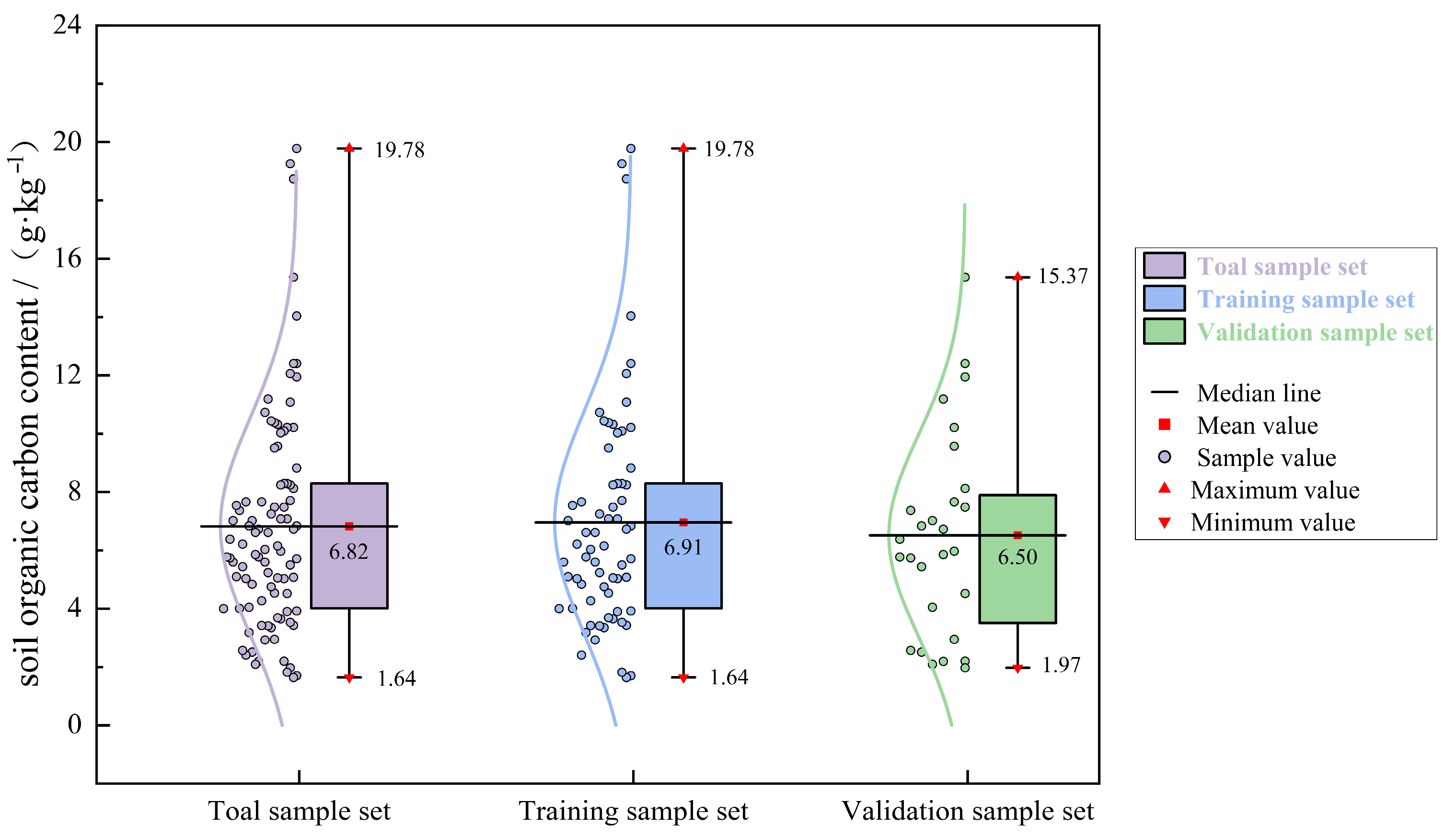
3.1. Soil Sample Characterization

Following the segmentation of the samples through the implementation of the SPXY method, the SOC content of the total sample set, in addition to the training and validation sets, underwent characterization. The ensuing results are presented in Figure 3. A thorough examination of the results reveals that the variability in SOC content within the cultivated layer of the Wei-Ku Oasis ranged from 1.64 to 19.78 g-per-kilogram, exhibiting pronounced spatial variations. The mean values of SOC for the total sample set, the training set, and the validation set were 6.82 g∙kg⁻¹, 6.91g∙kg⁻¹, and 6.50 g∙kg⁻¹, respectively. Statistical tests demonstrated that there were no significant differences in the mean values of SOC for these three sample sets (p > 0.05). The standard deviations of the three ranged from 3.488 to 3.852, and the dispersion between the sample sets was relatively close. The coefficient of variation, a measure of spatial heterogeneity within the samples, exhibited moderate strength in all three sample sets, with a value of approximately 54%. The preceding analysis demonstrates that the sample sets divided by the SPXY method exhibit adequate consistency in the distribution of SOC content. Furthermore, the training set, validation set, and total sample set display analogous statistical characteristics, thereby establishing a reliable data foundation for constructing a high-precision SOC prediction model.

3.2. Screening of Relevant Variables

In this study, the Boruta algorithm, the Lasso regression algorithm, and the Boruta–Lasso combination algorithm were employed to screen the original variable set for features, with the objective of optimizing the model performance. As demonstrated in Figure 4, the unscreened variable set encompasses a total of 30 variables, encompassing 13 spectral indices, 3 topographic parameters, 6 meteorological variables, 7 soil attributes, and 1 anthropogenic activity factor (TLU) multidimensional feature. The variable set screened by the Boruta algorithm retained all the spectral index variables and meteorological factors (BSE) and most of the soil attribute variables and the TLU, totaling 20 variables. The topographic parameters, most of the meteorological variables, and some of the soil attributes were excluded. The variable sets retained by the Lasso screening method included only 12 variables, primarily the spectral indices DVI, BI, and NDSI, the topographic variable Aspect, and the meteorological variables ET, ST, and BSE, as well as the soil attributes GVP, ClC, BD, EC, and TLU. Redundant spectral indices and some topographic and meteorological variables were excluded from the final analysis. The application of the Boruta–Lasso method, a hierarchical screening approach, led to the identification of seven core variables, including spectral indices such as DVI, BI, and NDSI, as well as BSE, ClC, BD, and TLU. This process involved the exclusion of secondary features such as Aspect, ET, ST, GVP, and EC. Boruta has been observed to retain multidimensional, ecologically relevant variables, Lasso has been demonstrated to prioritize reducing covariance, and the combined approach effectively balances the explanatory power of the variables and model simplicity through the two-stage screening, which provides a highly robust feature subset for subsequent modeling. Set I means the unfiltered variable set, Set II denotes the set of variables screened by the Boruta algorithm, Set III represents the set of variables screened by the Lasso algorithm, and Set IV shows the set of variables screened by the combination of the Boruta–Lasso algorithms.

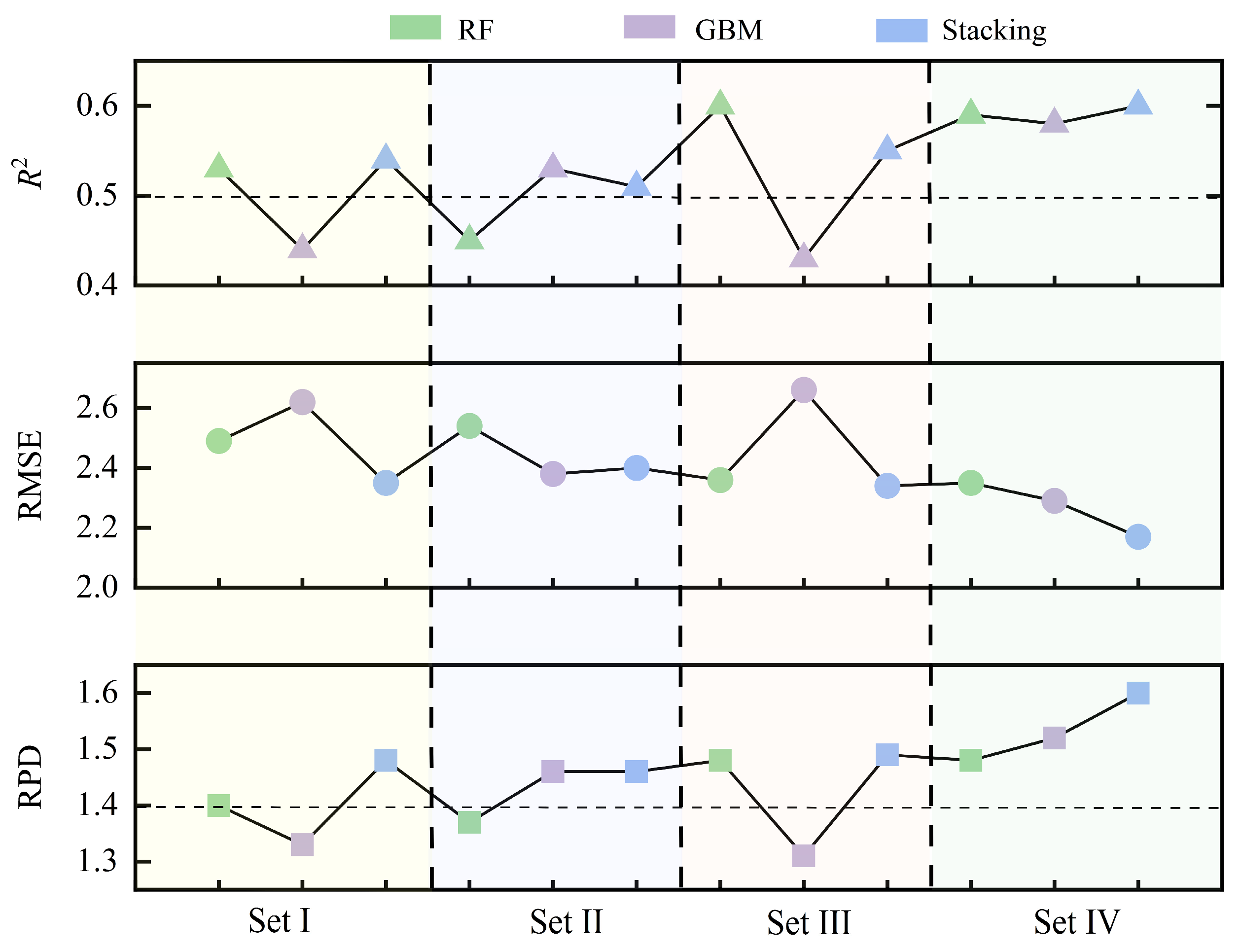
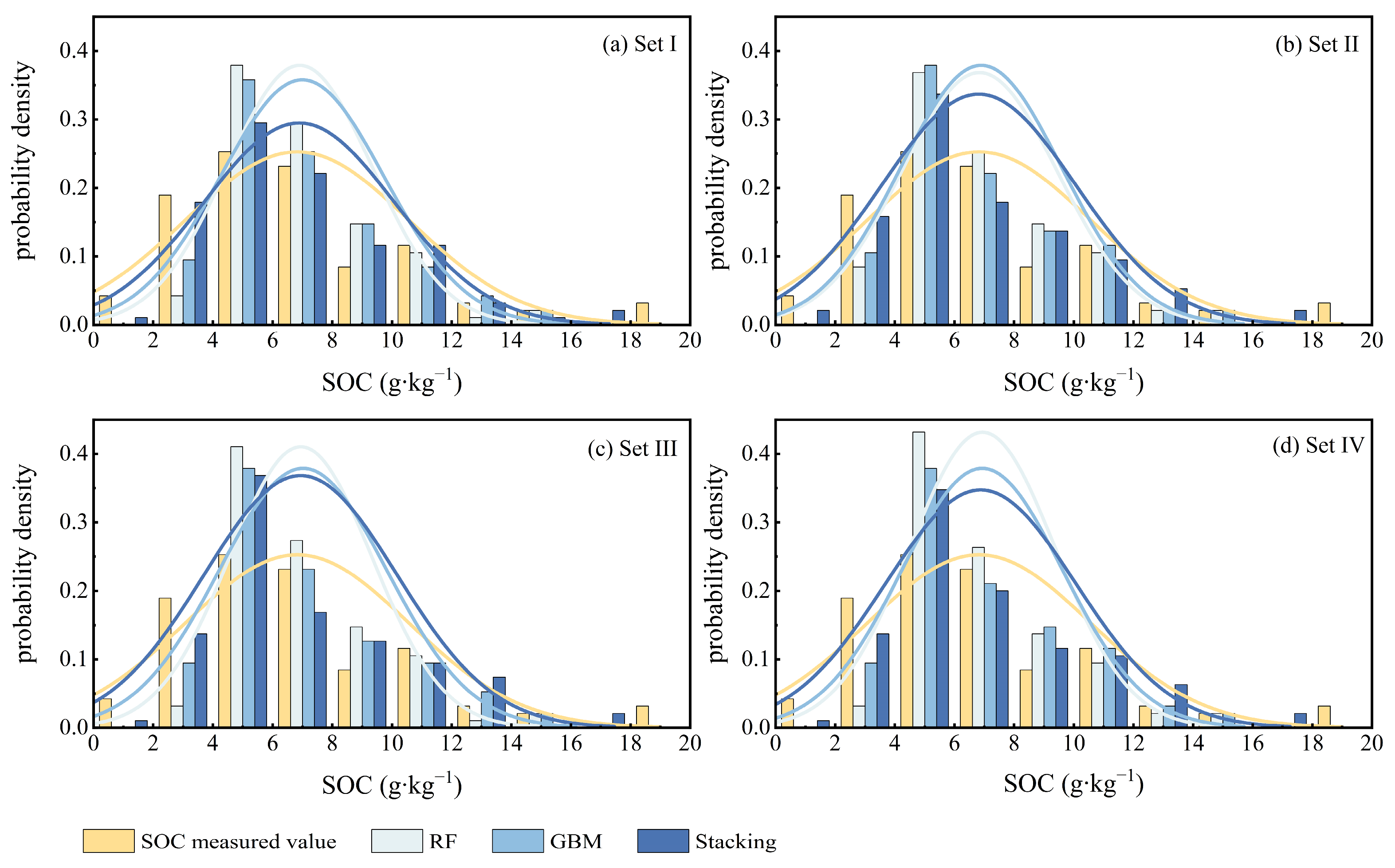
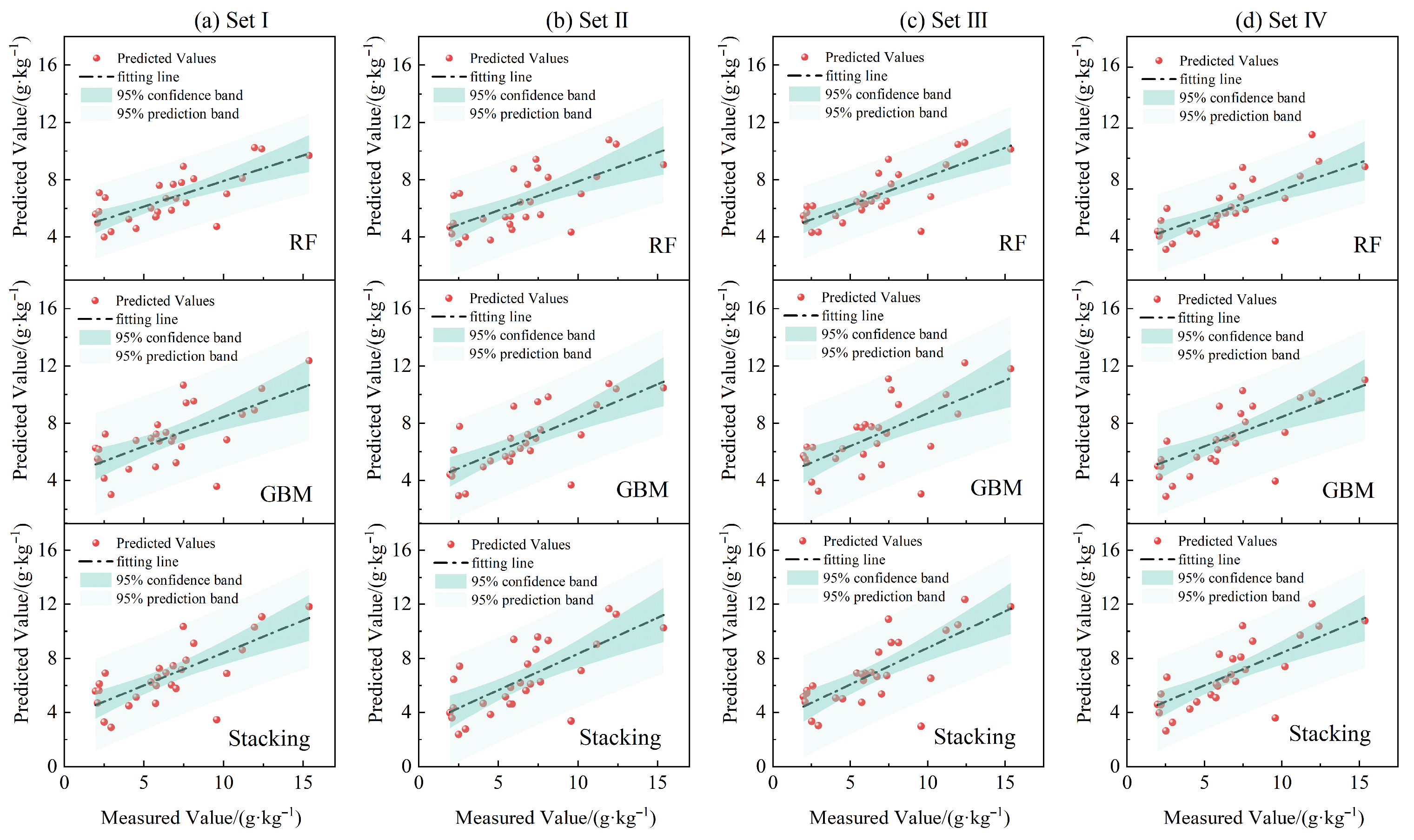
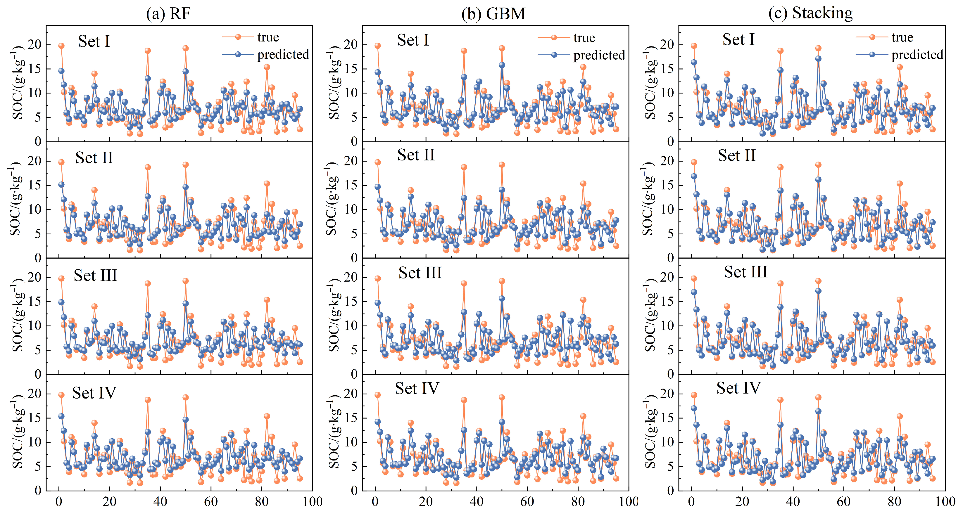
3.3. Estimation Modeling and Prediction Accuracy Evaluation

To ensure optimal model performance and stability, all model parameters were determined through multiple rounds of experimental testing and internal validation. This allowed each model to fully utilize its algorithmic strengths while reducing the risk of overfitting and enhancing generalization. In this study, RF, GBM, and Stacking models were constructed in RStudio (2024.12.0+467), where the RF model sets the number of trees ‘ntree = 1000’ through the ‘randomForest’ package, and the number of features-per-tree split is set to ‘mtry = sqrt(p)’ (p is the number of features); the GBM utilizes the ‘caret’ tuning parameter to fix the interaction depth (‘interation.depth = 3’), number of trees (‘n.trees = 300’), and learning rate (‘shrink-age = 0.02’), and optimized the parameters by 5-fold cross-validation; while the Stacking model takes the predicted values of RF and GBM as feature inputs, integrates the training with ridge regression as the metamodel, and selects the optimal orthogonal model by ‘cv.glmnet’ to select the optimal regularization parameters ‘lambda.min’. After multiple cycles of debugging and continuous tuning of base model parameters, as well as the optimization of Stacking feature combinations, three evaluation metrics (R², RMSE, and RPD) of both the training and test sets attain the optimal level under the current data and model structure.

As illustrated in

Table 3. Comparison of training set models accuracy.

Variable Set	Screening Methods	Model	R2	RMSE	RPD
Set I	Unfiltered	RF	0.91	1.50	2.57
		GBM	0.90	1.41	2.75
		Stacking	0.91	1.13	3.41
Set II	Boruta	RF	0.90	1.46	2.64
		GBM	0.88	1.53	2.53
		Stacking	0.90	1.21	3.18
Set III	Lasso	RF	0.91	1.57	2.45
		GBM	0.88	1.47	2.62
		Stacking	0.90	1.20	3.21
Set IV	Boruta–Lasso	RF	0.89	1.59	2.43
		GBM	0.85	1.62	2.38
		Stacking	0.89	1.31	2.95

, the training set results of the models with different variable sets are presented. The analysis indicates that the RF and Stacking models demonstrate higher estimation accuracy compared to the GBM model across all four variable sets, exhibiting superior generalization ability. The R² of multiple models constructed with different variable sets exceeds 0.85, the RMSE is less than 1.65 g·kg⁻¹, and the RPD is greater than 2.0, suggesting that the constructed models possess high estimation accuracy and stable prediction ability. A subsequent examination of the findings from the test set (see Figure 5) indicates that most of the constructed models exhibit R² values greater than 0.5 and RPD values exceeding 1.4. It indicates that these models all have high predictive stability and can accurately predict SOC. Especially in Set III and Set IV, the R² values of the RF and Stacking model are similar and relatively high. This indicates that, under this variable set, the predicted values of the two models align well with the measured values. In terms of RMSE metrics, the Stacking model for the Set IV variable set demonstrated the most optimal performance, exhibiting the highest prediction accuracy among all screening methods. This error was reduced by 10% in comparison to the Set I model. As for the RPD indicator, the Stacking model also performs well in Set IV, with an RPD of 1.61 which is closer to the excellence threshold of 2.0, indicating that the model’s prediction results are more stable and its prediction accuracy is better than that of other models. The results of this study indicate that, across a range of variables, the accuracy of the Stacking model consistently outperforms that of the RF and GBM models. Notably, the Stacking model demonstrates the most optimal performance among the models evaluated in Set IV.

Combined with the comparative analysis of the test set results (Figure 5), it is concluded that the degree of dependence of the feature variables on the training data determines the stability of the model as well as the model’s ability to adapt and generalize to the data. By comparing the modeling results of different variable sets, it is found that although the unscreened variable Set I performs outstandingly in the training set (R² = 0.91 for the optimal Stacking model), the R² of the test set decreases by 37%, and the risk of overfitting is significant; after screening by Boruta’s algorithm, the R²s of the RF and Stacking model in the variable set model of Set II drop dramatically from 0.90 and 0.90 in the training set to 0.45 and 0.51 in the test set, respectively; the models constructed in Set III of the Lasso screening variable set have stronger generalization ability but the test results perform poorly, in which the R² of the RF model decreases from 0.91 in the training set to 0.60 in the test set; the Set IV variable set shows the results of the screening of the combination of the two algorithms, in which the three models all have stable and good training results in this variable set and both R² and RPD in the test set are significantly higher than the other variable sets and the RMSE also shows high estimation accuracy. Specifically, the Stacking model performed the best, and the test set RMSE = 2.17g·kg⁻¹ achieved the minimum. In summary, it is concluded that the Boruta screening algorithm is prone to retain variables that are sensitive to the noise of the training set, while the Lasso regression method may ignore the potential higher-order interaction features among variables, and the combination of the Boruta and Lasso regression screening algorithms effectively balances the model’s fitting ability and generalization performance. The Stacking model has a reliable prediction performance in both the training set and the test set and a better generalization ability in both the training and test sets.

Figure 6 shows the Gaussian fitting curves of the SOC content of soil samples in different variable sets and different models. In the region of peak SOC distribution, the Gaussian fitting curves of the Stacking model in all the four variable sets were the closest to the measured values, indicating that its prediction accuracy was significantly better than that of the single ensemble model in the typical SOC intervals. Among the fitted curves for different sets of variables, the predicted values of the RF model constructed by Set II have the largest deviations from the measured values at the left and right sides of the peak, a phenomenon that is consistent with the results in the model evaluation metrics. In addition, the analysis of the prediction effects of Set III and Set IV shows that the Stacking model exhibits optimal fitting performance in the low, medium, and high SOC intervals, and the average absolute error of its prediction curves from the measured values is reduced compared to the other models. Therefore, the Stacking model constructed by Set IV showed the best performance in estimating the SOC content in the study area compared to other models. Furthermore, as shown in Figure 7 which presents the standardized residual plots of the RF, GBM, and Stacking models across the four datasets, the standardized residuals were randomly distributed around the zero-line relative to the standardized predicted values. This random distribution indicates that neither under-prediction nor over-prediction systematically occurred in any of the models. In terms of prediction stability, the average standardized deviations of each model across different datasets showed remarkable consistency, with absolute values ranging from 0.66 to 0.71. The minimum deviations for all these models were close to zero, while the maximum deviations were approximately 3.5. Among them, the Stacking Set IV model demonstrated the best overall prediction consistency and had strong generalization capabilities.

The estimation results of RF, GBM, and Stacking models in four variable sets are shown in Figure 8. For the RF model, the distribution of predicted values in Set I is more dispersed, with large deviation from the fitting line, wider confidence and prediction bands, and limited stability and accuracy. After variable screening the degree of predicted value aggregation of the RF model is improved, but the optimization magnitude is not significant relative to other models. The discrete nature of the predicted values is obvious when the GBM model is not screened, and the degree of aggregation of the predicted values and the stability of the model are gradually enhanced after the processing of each screening method but the overall optimization effect still has a gap compared with the Stacking model. In the Stacking model, the predicted values are more discrete in Set I. However, after both screening methods the predicted value concentration tendency gradually improves, especially after the combination of screening causing the predicted values to be tightly clustered around the fitting line, the discrete points to be reduced substantially, and the 95% confidence bands and the pre-diction bands to be significantly narrowed, which shows that the model has the optimal fitting accuracy and stability for the validation set. In summary, the Boruta algorithm is based on RF to assess the importance of variables, and the Lasso screening method is used to eliminate redundant variables through regularization. Therefore, the combination of the two can not only retain the key variables but also eliminate the covariance between the variables and noise interference. Under the framework of the Stacking model this indicates that the combination of the Boruta and Lasso screening methods has a greater advantage in improving the model generalization ability and prediction accuracy.

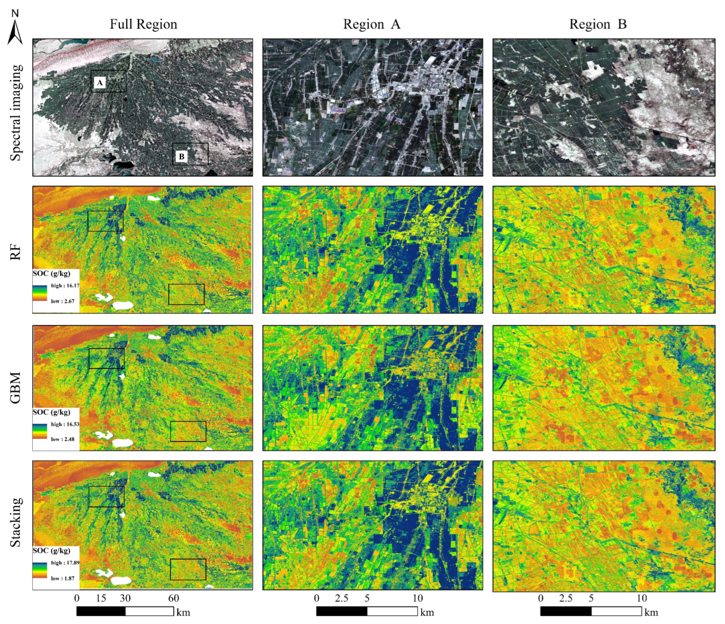
3.4. Comparison of SOC Spatial Prediction Results

The RF, GBM, and Stacking models developed using the optimal variable set (Set IV) were applied to perform spatial prediction of SOC in the study area (Figure 9).

Among the three models, the Stacking model exhibited the highest prediction accuracy, followed by GBM, while RF showed relatively lower accuracy. Prediction maps indicated that the three models generally agreed on the overall trends of SOC spatial distribution predictions, although minor discrepancies emerged in localized areas. In high-SOC regions (Figure 9A), GBM yielded the highest predictions, followed by the Stacking model, with RF providing the lowest estimates. Conversely, in low-SOC regions (Figure 9B), GBM predictions were the lowest, the Stacking model’s predictions were intermediate, and RF predictions trended higher. This pattern can be attributed to GBM’s heightened sensitivity to numerical variations, which amplifies prediction disparities, whereas RF favors conservative predictions, exhibiting a “compression” effect on extreme values. Although the Stacking model’s predictions typically fell between those of GBM and RF across regions, it uniquely captured SOC extreme values in the study area’s overall prediction maps. This suggests that the Stacking model not only enables stable regional predictions but also demonstrates a strong capability to identify extreme values. Collectively, while the three models exhibit distinct advantages in different contexts, the Stacking ensemble model excels in prediction accuracy and adaptability to complex scenarios, enabling precise SOC prediction in the study area.

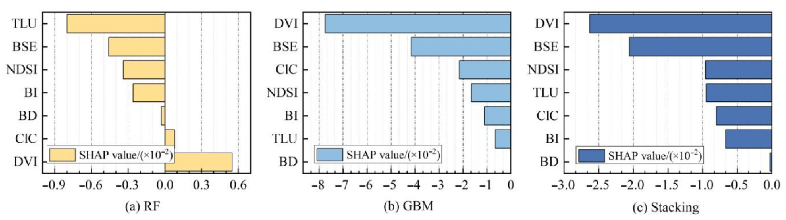
3.5. Importance Analysis of Characteristic Variables

The SHAP analysis results in Figure 10 showed that the importance of the seven characteristic variables in different algorithmic models showed some differences, indicating that the key factors also had the ability to predict SOC. For instance, where the weighting coefficients α and β are 0.86 and 0.40 for the RF and GBM models, respectively. In the RF model, DVI (Difference Vegetation Index) was the most dominant positive variable with a SHAP value of 0.55 × 10⁻², indicating that vegetation cover had a significant contribution to SOC accumulation. In contrast, in the GBM model, DVI showed a strong negative variable (SHAP value −7.74 × 10⁻²), which may be related to the presence of severe salinization phenomenon and the low-carbon characteristics of soil in some high DVI areas of the study area. This contrast can be attributed to differences in algorithm mechanisms and the spatial heterogeneity of the study area. RF, as a bagging-based ensemble, reflects overall trends, while GBM, as a boosting model, is more sensitive to local residuals. In salinized areas with dense but degraded vegetation, high DVI values may correspond to low SOC values, which is more strongly captured by GBM. In addition, BSE had SHAP values of −4.16 × 10⁻² and −2.06 × 10⁻² in the GBM and Stacking models, respectively, reflecting the inhibitory effect of water stress on SOC accumulation. The TLU, as an important variable, showed a stable negative contribution in all three models, with a SHAP value of −0.95 × 10⁻² in the Stacking model, indicating that LU changes had a significant effect on the SOC distribution, especially after a large amount of cultivated land was transformed into garden land, as was found in the field survey. In this scenario the SOC content showed a decreasing trend, which further corroborated of the reliability of the results of the model analysis. The SHAP values of the Stacking model were obtained by weighting the Ridge regression on the SHAP results of the RF and GBM models, which can synthesize the explanatory ability of the sub-models more comprehensively. Overall, DVI, BSE, and TLU are the most representative key variables in the three models, and the differences in the direction and magnitude of their contributions further suggest that the spatial variation in SOC is driven by multifactor interactions.

4. Discussion

4.1. Integrated Assessment of Screening Methods and Model Performance

In the process of feature variable screening, although Boruta can comprehensively retain multidimensional features and the training set performs well, it may introduce redundant information due to the high dimensionality of the variables, resulting in the weakening of the contribution of some of the variables to the prediction of the SOC which in turn affects the model’s ability to generalize. The Lasso method can lead to feature over-rejection problems when dealing with multi-source remote sensing data. The Boruta and Lasso combination screening retains sufficient information to avoid underfitting in the training set and achieves optimal performance in the test set, and the variable set combines both ecological interpretability and model simplicity [48,49]. The results of this study show (Figure 11) that the combination of Boruta and Lasso screening methods performs superiorly in estimating SOC content, retaining multidimensional ecological features through Boruta’s algorithm to avoid the omission of potentially important variables, and using Lasso algorithm’s L1 regularization to eliminate redundant variables and reduce covariance. The two complement each other to effectively improve the explanatory power and generalization performance of the model. The constructed Stacking model has a maximum improvement of 18% and 10.3% over the R²s and RPDs of the single screening methods for the test set. Furthermore, the RMSE is reduced by 9.3% and the model’s generalization ability and prediction accuracy are both superior.

For the three algorithms RF, GBM, and Stacking, this study systematically explores the effects of different feature screening methods on model performance, and the results are shown in Figure 10. The modeling accuracy of feature variable screening was improved to a greater extent than that of non-screening; the fit between the predicted values and the real values of each model was significantly improved, especially in Set IV; the model fit was better; and the distribution trend of the predicted values and the real values was more consistent. Together these indicated that the variable screening could optimize the performance of the model and improve the accuracy of the prediction of the organic carbon content of the soil. Among them, the RF model has a test set R² of up to 0.60 in Set III, which shows good adaptability to redundant variable removal, but the prediction effect decreases in Set IV instead, indicating that the model needs to carefully balance the retention and removal of variables. The GBM model is significantly dependent on Set IV, and the R² of the test set is improved from the initial 0.44 to 0.58, which effectively alleviates the overfitting problem. The Stacking model achieved optimal performance under the combined screening approach with the test set R² reaching 0.61 and the RMSE decreasing to 2.17 g·kg⁻¹, an 18% improvement in R² and a 9.3% reduction in RMSE compared to Boruta’s single screening, which fully reflects the high sensitivity of the ensemble model to the feature variables. The Stacking model is able to take full advantage of different algorithms by integrating multiple base learners and optimizing the prediction results using meta-learners [50]. Zhou et al. [51] constructed a hyperspectral estimation model for SOC content prediction by combining algorithms such as RF and multiple linear regression after implementing spectral transform preprocessing on the raw spectra. The results show that the RF model performs optimally in terms of overall simulation accuracy. It indicates that the RF model is superior in the strong spectral–carbon content correlation scenario by virtue of the feature importance ranking ability, while the Stacking model demonstrates stronger adaptability in a weak-signal and high-noise environment. In addition, this study suppresses overfitting by means of cross-validation and regularization, but the model still suffers from training–testing set performance discrepancy, which may be attributed to the heterogeneity of feature selection methods (e.g., Boruta vs. Lasso). This results in a feature subset that is sensitive to the specificity of the training data, which constrains the applicability of the model. Subsequent studies will start to further explore the screening of feature variables and model hyperparameter optimization to enhance the robustness and generalization performance of the model [52].

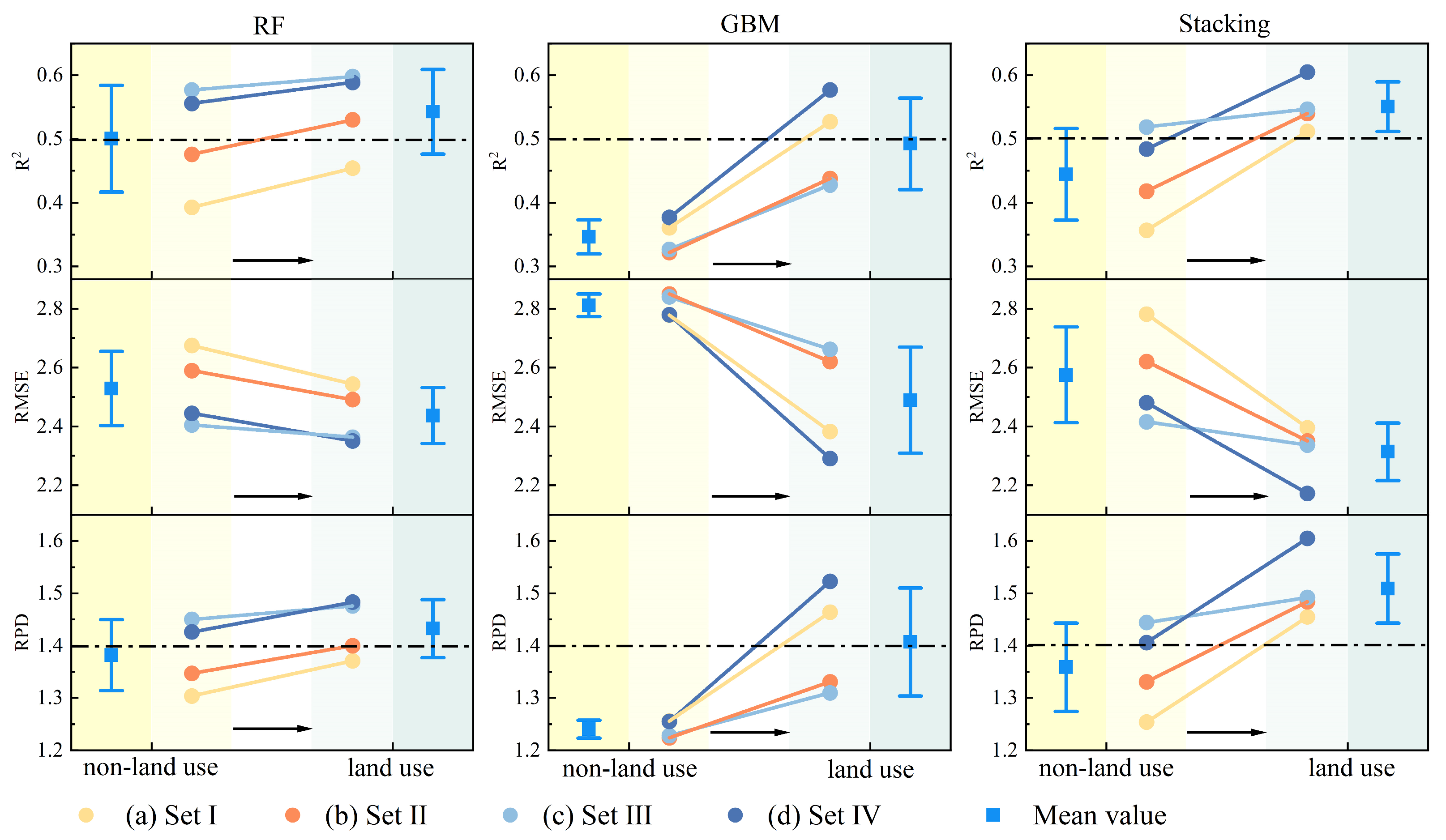
4.2. Impact of LU Data on Model Performance

SOC content is highly susceptible to changes in climate, hydrology, geography (e.g., microtopography and geomorphology), soil conditions (including type of parent material, texture and thickness of soil layers, etc.), and vegetation, and LU modes [53,54,55]. The observed improvements in model performance when including LU data likely reflect the integrated effects of vegetation-mediated carbon inputs, microbial decomposition processes, and land management practices that collectively shape SOC dynamics [56]. Wang et al. [57] found that differences in land surface cover types have significant regulatory effects on the spatial patterns of SOC, with the underlying mechanisms attributed to variations in key processes such as litter input flux, organic matter decomposition rate, and the intensity of human disturbances under different TLU. Guo et al. [58] showed that ML approaches (e.g., RF) integrating multi-source covariates (e.g., terrain, climate, soil properties) can effectively model the spatial distribution of SOC density in cultivated lands. This study investigates how LU data enhances predictive modeling through controlled experiments comparing the RF, GBM, and Stacking models with versus without LU data inclusion, quantitatively assessing its effects on model performance improvement. The enhanced model accuracy with LU data incorporation can be attributed to its capacity to represent the complex interplay between vegetation characteristics, soil management practices, and associated biogeochemical processes that collectively determine SOC accumulation and stabilization. By comparing modeling performance across different feature screening methods, the results are shown in Figure 12. It is found that in the case of including LU data, the R² and RPD of all three models are improved, and the RMSE shows a decreasing trend. In particular, the GBM and Stacking models have substantial improvements in different variable sets, especially in the model with Boruta and Lasso combination screening, indicating that the LU data can improve the model fitting excellence, reduce the error, and enhance the prediction ability. Specifically, the Stacking model improves R² and RPD by 24% and 14%, respectively, and reduces RMSE by 13% in Set IV, which fully reflects the synergistic effect of the feature screening variables. The GBM model improves R² by 54% and reduces RMSE by 18% in Set IV, which effectively mitigates the sensitivity to high-dimensional data. The RF model improves R² by 4% in Set III, which complements the key spatial features. In addition, when LU data are included, the R² of the constructed model is mostly greater than 0.5, which indicates that there is a more significant linear relationship between the independent variables and the dependent variable, and it has a certain fitting ability to the data; at the same time, most of the RPD exceeds 1.4, which indicates that the model has a medium-or-above prediction ability and that it can make reasonable predictions to the unknown data. LU data significantly reduces the risk of model overfitting, especially in the Stacking model of Set IV where the R² difference between the training set and the test set is 32% after the introduction of LU data, which is 17% smaller than that in the absence of LU data. This study confirms that incorporating TLU variables can offer more precise background information on LU. This, in turn, enhances the model’s explanatory power and predictive accuracy regarding the spatial differentiation of SOC. Significant disparities exist among different TLUs (cultivated land, garden land, and unutilized land) in terms of vegetation coverage, root biomass, and the extent of human interference. These differences directly influence the accumulation and decomposition processes of SOC. Under conditions of substantial litter input and artificial fertilization, garden land maintains relatively high SOC content. Frequent agricultural activities in cultivated land accelerate the release of SOC. In contrast, due to the absence of continuous biological substance input and a low level of human intervention, the accumulation rate of SOC in unutilized land is relatively slow. Moreover, TLU data can enrich feature diversity, facilitate feature interaction, mitigate redundant noise, and notably improve model performance [28]. Especially in integrated models, it provides a crucial reference for high-dimensional data modeling.

4.3. Limitations and Future Work

This study takes the spatial prediction of SOC in the Wei-Ku Oasis as an example to verify the feasibility and effectiveness of the comprehensive modeling framework of ensemble learning in the spatial prediction of SOC in oasis farmland in arid areas. However, several technical limitations still exist. The 95 samples used generally met the requirements for overall modeling, yet they were insufficient for reflecting the complex spatial variability within the study area. This, to a certain extent, affected the robustness of the model. Moreover, in highly heterogeneous areas, such as the edges of irrigation canals and salinized plots, the distribution of sample points was relatively sparse, making it difficult to depict the detailed changes in actual soil characteristics. Meanwhile, soil properties usually exhibit obvious spatial autocorrelation. Nevertheless, the currently adopted SPXY sample partitioning method and the model training process do not explicitly account for this spatial correlation, which may impact the prediction accuracy of local regions [59]. Although this study divided the dataset into a training set and a validation set for model construction and evaluation, there was an overall lack of independent on-site validation, limiting the comprehensive assessment of the model’s generalization ability [60]. Future research could introduce spatial hierarchical sampling methods to enhance the representativeness of samples across different ecological communities [61]. Additionally, the universality of this model is subject to certain limitations. The Wei-Ku Oasis mainly relies on artificial irrigation, and agricultural activities are relatively frequent. The distribution of SOC is significantly influenced by human factors such as fertilization and irrigation. Therefore, when directly applying the model to agricultural areas dominated by natural precipitation, special attention should be paid to the influence of factors such as farming and irrigation methods on the spatial distribution of SOC.

Although the Stacking model demonstrated strong generalization ability in this study, the improvement in its performance might mainly be attributed to the meta-learner’s integration of the predictive ability of the basic models through regularization to reduce the risk of overfitting. However, the effectiveness of Stacking highly depends on the differences and complementarities among the base models. Once the base models converge in structure or performance, the integration effect of the meta-learning layer will be significantly weakened [62]. Furthermore, when the sample size is limited or feature redundancy is high, the complex structure and numerous parameters of Stacking will instead lead to error accumulation. Therefore, its generalization advantage is not absolute as it is highly sensitive to modeling methods, data structures, and model parameters, and further verification in practice is needed [63]. From a practical application perspective, the 10 m spatial resolution organic carbon prediction model constructed in this study has identified the low-organic carbon risk areas of the oasis with a certain degree of accuracy. It is of great significance for regional farmland nutrient regulation and soil health evaluation and also provides scientific support for the establishment of an agricultural comprehensive governance system of “monitoring-early warning-precise management”.

5. Conclusions

This study presents a methodological framework combining Sentinel-2A images, environmental data, and ground investigations. We constructed a multidimensional feature space containing spectral features, topographic factors, meteorological elements, soil properties, and TLUs by Boruta algorithm, Lasso regression, and their combination screening methods. When combined with RF, GBM, and Stacking models the SOC content of the oasis cultivated layer in the arid zone was accurately estimated and mapped. The main conclusions are as follows:

(1) The feature variable Set IV screened based on the combined Boruta and Lasso algorithm significantly improves the prediction accuracy of the model. This variable set contains three key spectral indices, DVI, BI, and NDSI, as well as the meteorological factor BSE, the soil attributes ClC and BD, and TLU, and the performance of the model constructed by it is significantly better than the results of single feature selection.

(2) The variable screening based on the combined algorithm of Boruta and Lasso overcomes the issues of the high redundancy of feature variables and the poor generalization ability of single models in traditional spatial prediction methods for soil organic carbon. The Stacking model constructed using this combined screening method demonstrates the optimal prediction performance. By integrating remote sensing technologies with ground investigation methods and considering relevant variables, such as land use types, we can accurately estimate the carbon sink of fragile ecosystems in arid regions. This approach provides technical support for ecological protection and carbon sink research in arid areas.

References

1. Carvalhais, N.; Forkel, M.; Khomik, M.; Bellarby, J.; Jung, M.; Migliavacca, M.; Μu, M.; Saatchi, S.; Santoro, M.; Thurner, M.; et al. Global covariation of carbon turnover times with climate in terrestrial ecosystems. Nature 2014, 514, 213–217. [Google Scholar] [CrossRef]
2. Bhattacharya, S.S.; Kim, K.H.; Das, S.; Uchimiya, M.; Jeon, B.H.; Kwon, E.; Szulejko, J.E. A review on the role of organic inputs in maintaining the soil carbon pool of the terrestrial ecosystem. J. Environ. Manag. 2016, 167, 214–227. [Google Scholar] [CrossRef] [PubMed]
3. Nayak, A.K.; Rahman, M.M.; Naidu, R.; Dhal, B.; Swain, C.K.; Nayak, A.D.; Tripathi, R.; Mohammad Shahid, M.; Islam, M.R.; Pathak, H. Current and emerging methodologies for estimating carbon sequestration in agricultural soils: A review. Sci. Total Environ. 2019, 665, 890–912. [Google Scholar] [CrossRef]
4. Abdulraheem, M.I.; Zhang, W.; Li, S.; Moshayedi, A.J.; Farooque, A.A.; Hu, J. Advancement of remote sensing for soil measurements and applications: A comprehensive review. Sustainability 2023, 15, 15444. [Google Scholar] [CrossRef]
5. Lin, N.; Quan, H.; He, J.; Li, S.; Xiao, M.; Wang, B.; Chen, T.; Dai, X.; Pan, J.; Li, N. Urban vegetation extraction from high-resolution remote sensing imagery on SD-UNet and vegetation spectral features. Remote Sens. 2023, 15, 4488. [Google Scholar] [CrossRef]
6. Li, T.; Cui, L.; Wu, Y.; McLaren, T.I.; Xia, A.; Pandey, R.; Liu, H.; Wang, W.; Xu, Z.; Song, X.; et al. Soil organic carbon estimation via remote sensing and machine learning techniques: Global topic modeling and research trend exploration. Remote Sens. 2024, 16, 3168. [Google Scholar] [CrossRef]
7. Rodrigues, E.; Gomes, Á.; Gaspar, A.R.; Antunes, C.H. Estimation of renewable energy and built environment-related variables using neural networks–A review. Renew. Sustain. Energy Rev. 2018, 94, 959–988. [Google Scholar] [CrossRef]
8. Vohland, M.; Besold, J.; Hill, J.; Fründ, H.C. Comparing different multivariate calibration methods for the determination of soil organic carbon pools with visible to near infrared spectroscopy. Geoderma 2011, 166, 198–205. [Google Scholar] [CrossRef]
9. Tan, Q.; Geng, J.; Fang, H.; Li, Y.; Guo, Y. Exploring the impacts of data source, model types and spatial scales on the soil organic carbon prediction: A case study in the red soil hilly region of southern China. Remote Sens. 2022, 14, 5151. [Google Scholar] [CrossRef]
10. Dos Santos, U.J.; De Melo Dematte, J.A.; Menezes, R.S.C.; Dotto, A.C.; Guimarães, C.C.B.; Alves, B.J.R.; Primo, D.C.; Sampaio, E.V.D.S.B. Predicting carbon and nitrogen by visible near-infrared (Vis-NIR) and mid-infrared (MIR) spectroscopy in soils of Northeast Brazil. Geoderma Reg. 2020, 23, e00333. [Google Scholar] [CrossRef]
11. Cambou, A.; Barthès, B.G.; Moulin, P.; Chauvin, L.; Faye, E.H.; Masse, D.; Chevallier, T.; Chapuis-Lardy, L. Prediction of soil carbon and nitrogen contents using visible and near infrared diffuse reflectance spectroscopy in varying salt-affected soils in Sine Saloum (Senegal). Catena 2022, 212, 106075. [Google Scholar] [CrossRef]
12. Zhang, Y.; Shen, H.; Gao, Q.; Zhao, L. Estimating soil organic carbon and pH in Jilin Province using Landsat and ancillary data. Soil Sci. Soc. Am. J. 2020, 84, 556–567. [Google Scholar] [CrossRef]
13. Xiao, X.; He, Q.; Ma, S.; Liu, J.; Sun, W.; Lin, Y.; Yi, R. Environmental variables improve the accuracy of remote sensing estimation of soil organic carbon content. Sci. Rep. 2024, 14, 18964. [Google Scholar] [CrossRef]
14. Ho, V.H.; Morita, H.; Bachofer, F.; Ho, T.H. Random forest regression kriging modeling for soil organic carbon density estimation using multi-source environmental data in central Vietnamese forests. Model. Earth Syst. Environ. 2024, 10, 7137–7158. [Google Scholar] [CrossRef]
15. Cutler, A.; Cutler, D.R.; Stevens, J.R. Random forests. In Ensemble Machine Learning: Methods and Applications; Springer: New York, NY, USA, 2012; pp. 157–175. [Google Scholar] [CrossRef]
16. Natekin, A.; Knoll, A. Gradient boosting machines, a tutorial. Front. Neurorobotics 2013, 7, 21. [Google Scholar] [CrossRef] [PubMed]
17. Healey, S.P.; Cohen, W.B.; Yang, Z.; Brewer, C.K.; Brooks, E.B.; Gorelick, N.; Hernandez, A.J.; Huang, C.; Hughes, M.J.; Kennedy, R.E.; et al. Mapping forest change using stacked generalization: An ensemble approach. Remote Sens. Environ. 2018, 204, 717–728. [Google Scholar] [CrossRef]
18. Azizi, K.; Ayoubi, S.; Demattê, J.A. Controlling factors in the variability of soil magnetic measures by machine learning and variable importance analysis. J. Appl. Geophys. 2023, 210, 104944. [Google Scholar] [CrossRef]
19. Keskin, H.; Grunwald, S.; Harris, W.G. Digital mapping of soil carbon fractions with machine learning. Geoderma 2019, 339, 40–58. [Google Scholar] [CrossRef]
20. Xie, B.; Ding, J.; Ge, X.; Li, X.; Han, L.; Wang, Z. Estimation of soil organic carbon content in the Ebinur Lake wetland, Xinjiang, China, based on multisource remote sensing data and ensemble learning algorithms. Sensors 2022, 22, 2685. [Google Scholar] [CrossRef]
21. Muñoz, A.S.M.; Alvis, Á.I.G.; Martínez, I.F.B. A random forest model to predict soil organic carbon storage in mangroves from Southern Colombian Pacific coast. Estuar. Coast. Shelf Sci. 2024, 299, 108674. [Google Scholar] [CrossRef]
22. Wu, M.; Dou, S.; Lin, N.; Jiang, R.; Zhu, B. Estimation and mapping of soil organic matter content using a stacking ensemble learning model based on hyperspectral images. Remote Sens. 2023, 15, 4713. [Google Scholar] [CrossRef]
23. Tang, K.; Zhao, X.; Xu, Z.; Sun, H. A stacking ensemble model for predicting soil organic carbon content based on visible and near-infrared spectroscopy. Infrared Phys. Technol. 2024, 140, 105404. [Google Scholar] [CrossRef]
24. Bernardini, L.G.; Rosinger, C.; Bodner, G.; Keiblinger, K.M.; Izquierdo-Verdiguier, E.; Spiegel, H.; Retzlaff, C.O.; Holzinger, A. Learning vs. understanding: When does artificial intelligence outperform process-based modeling in soil organic carbon prediction? New Biotechnol. 2024, 81, 20–31. [Google Scholar] [CrossRef]
25. Li, S.; Li, X.; Ge, X. Prediction and mapping of soil organic carbon in the Bosten Lake oasis based on Sentinel-2 data and environmental variables. Int. Soil Water Conserv. Res. 2025, 13, 436–446. [Google Scholar] [CrossRef]
26. Li, Y.T.; Yang, R.M.; Zhang, X.; Xu, L.; Zhu, C.M. Understanding drivers of the spatial variability of soil organic carbon in China’s terrestrial ecosystems. Land Degrad. Dev. 2024, 35, 308–320. [Google Scholar] [CrossRef]
27. An, B.; Wang, X.; Huang, X. Changing characteristics, driving factors and future predictions of land use in the Weigan-Kuqa River Delta Oasis, China. Sci. Rep. 2024, 14, 29318. [Google Scholar] [CrossRef]
28. Adeniyi, O.D.; Maerker, M. Explorative analysis of varying spatial resolutions on a soil type classification model and its transferability in an agricultural lowland area of Lombardy, Italy. Geoderma Reg. 2024, 37, e00785. [Google Scholar] [CrossRef]
29. Gutman, G.G. Vegetation indices from AVHRR: An update and future prospects. Remote Sens. Environ. 1991, 35, 121–136. [Google Scholar] [CrossRef]
30. Jordan, C.F. Derivation of leaf-area index from quality of light on the forest floor. Ecology 1969, 50, 663–666. [Google Scholar] [CrossRef]
31. Mangewa, L.J.; Ndakidemi, P.A.; Alward, R.D.; Kija, H.K.; Bukombe, J.K.; Nasolwa, E.R.; Munishi, L.K. Comparative assessment of UAV and sentinel-2 NDVI and GNDVI for preliminary diagnosis of habitat conditions in Burunge wildlife management area, Tanzania. Earth 2022, 3, 769–787. [Google Scholar] [CrossRef]
32. Gurung, R.B.; Breidt, F.J.; Dutin, A.; Ogle, S.M. Predicting Enhanced Vegetation Index (EVI) curves for ecosystem modeling applications. Remote Sens. Environ. 2009, 113, 2186–2193. [Google Scholar] [CrossRef]
33. Veraverbeke, S.; Gitas, I.; Katagis, T.; Polychronaki, A.; Somers, B.; Goossens, R. Assessing post-fire vegetation recovery using red–near infrared vegetation indices: Accounting for background and vegetation variability. ISPRS J. Photogramm. Remote Sens. 2012, 68, 28–39. [Google Scholar] [CrossRef]
34. Purevdorj, T.S.; Tateishi, R.; Ishiyama, T.; Honda, Y. Relationships between percent vegetation cover and vegetation indices. Int. J. Remote Sens. 1998, 19, 3519–3535. [Google Scholar] [CrossRef]
35. Vieira, A.S.; Do Valle Junior, R.F.; Rodrigues, V.S.; da Silva Quinaia, T.L.; Mendes, R.G.; Valera, C.A.; Fernandes, L.F.S.; Pacheco, F.A.L. Estimating water erosion from the brightness index of orbital images: A framework for the prognosis of degraded pastures. Sci. Total Environ. 2021, 776, 146019. [Google Scholar] [CrossRef]
36. Li, S.; Yuan, F.; Ata-UI-Karim, S.T.; Zheng, H.; Cheng, T.; Liu, X.; Tian, Y.; Zhu, Y.; Cao, W.; Cao, Q. Combining color indices and textures of UAV-based digital imagery for rice LAI estimation. Remote Sens. 2019, 11, 1763. [Google Scholar] [CrossRef]
37. Mishra, M.; Singh, K.K.; Pandey, P.C.; Devrani, R.; Pandey, A.K.; Raju, K.P.; Ranjan, P.; Arora, A.; Costache, R.; Janizadeh, S.; et al. Spectral indices across remote sensing platforms and sensors relating to the three poles: An overview of applications, challenges, and future prospects. In Advances in Remote Sensing Technology and the Three Poles; Wiley & Sons: New York, NY, USA, 2022. [Google Scholar] [CrossRef]
38. Kandala, R.; Franssen, H.J.H.; Chaudhuri, A.; Sekhar, M. The value of soil temperature data versus soil moisture data for state, parameter, and flux estimation in unsaturated flow model. Vadose Zone J. 2024, 23, e20298. [Google Scholar] [CrossRef]
39. Chen, W.; Zeng, J. Decoupling analysis of land use intensity and ecosystem services intensity in China. J. Nat. Resour. 2021, 36, 2853–2864. [Google Scholar] [CrossRef]
40. Hu, Y.; Li, T. Forecasting Spatial Pattern of Land Use Change in Rapidly Urbanized Regions Based on SD-CA Model. Acta Sci. Nat. Univ. Pekin. 2022, 58, 372–382. [Google Scholar] [CrossRef]
41. Kursa, M.B.; Rudnicki, W.R. Feature selection with the Boruta package. J. Stat. Softw. 2010, 36, 1–13. [Google Scholar] [CrossRef]
42. Tibshirani, R. Regression shrinkage and selection via the lasso. J. R. Stat. Soc. Ser. B 1996, 58, 267–288. [Google Scholar] [CrossRef]
43. Chen, J.; Shen, C.; Xue, H.; Yuan, B.; Zheng, B.; Shen, L.; Fang, X. Development of an early prediction model for vomiting during hemodialysis using LASSO regression and Boruta feature selection. Sci. Rep. 2025, 15, 10434. [Google Scholar] [CrossRef] [PubMed]
44. Ekanayake, I.U.; Meddage, D.P.P.; Rathnayake, U. A novel approach to explain the black-box nature of machine learning in compressive strength predictions of concrete using Shapley additive explanations (SHAP). Case Stud. Constr. Mater. 2022, 16, e01059. [Google Scholar] [CrossRef]
45. Chen, W.; Chen, H.; Feng, Q.; Mo, L.; Hong, S. A hybrid optimization method for sample partitioning in near-infrared analysis. Spectrochim. Acta Mol. Biomol. Spectrosc. 2021, 248, 119182. [Google Scholar] [CrossRef]
46. Merabet, K.; Di Nunno, F.; Granata, F.; Kim, S.; Adnan, R.M.; Heddam, S.; Kisi, O.; Zounemat-Kermani, M. Predicting water quality variables using gradient boosting machine: Global versus local explainability using SHapley Additive Explanations (SHAP). Earth Sci. Inform. 2025, 18, 298. [Google Scholar] [CrossRef]
47. Wang, W.C.; Gu, M.; Li, Z.; Hong, Y.H.; Zang, H.F.; Xu, D.M. A stacking ensemble machine learning model for improving monthly runoff prediction. Earth Sci. Inform. 2025, 18, 120. [Google Scholar] [CrossRef]
48. Han, C.; Yang, G.; Wen, H.; Fu, M.; Peng, B.; Xu, B.; Yin, X.; Wang, P.; Zhu, L.; Feng, M. Development and validation of a quick screening tool for predicting neck pain patients benefiting from spinal manipulation: A machine learning study. Chin. Med. 2025, 20, 74. [Google Scholar] [CrossRef]
49. Fu, Y.; Zhao, J.; Wang, Y. LASSO regression and Boruta algorithm to explore the relationship between neutrophil percentage to albumin ratio and asthma: Results from the NHANES 2001 to 2018. Clin. Exp. Med. 2025, 25, 149. [Google Scholar] [CrossRef]
50. Cui, Z.; Chen, S.; Hu, B.; Wang, N.; Feng, C.; Peng, J. Mapping Soil Organic Carbon by Integrating Time-Series Sentinel-2 Data, Environmental Co-variates and Multiple Ensemble Models. Sensors 2025, 25, 2184. [Google Scholar] [CrossRef]
51. Zhou, W.; Cao, X.; Wang, K.; Xiao, J.; Wang, T.; Li, H.; Ji, C. Hyperspectral modeling of soil organic carbon content-a case study of the Sanjiangyuan region of the Qinghai-Tibet Plateau. J. Glaciol. Geocryol. 2023, 45, 823–832. [Google Scholar] [CrossRef]
52. Chai, X.; Li, S.; Liang, F. A novel battery SOC estimation method based on random search optimized LSTM neural network. Energy 2024, 306, 132583. [Google Scholar] [CrossRef]
53. Guo, M.; Yang, L.; Zhang, L.; Shen, F.; Meadows, M.E.; Zhou, C. Hydrology, vegetation, and soil properties as key drivers of soil organic carbon in coastal wetlands: A high-resolution study. Environ. Sci. Ecotechnol. 2025, 23, 100482. [Google Scholar] [CrossRef]
54. Luo, Z.; Wang, G.; Wang, E. Global subsoil organic carbon turnover times dominantly controlled by soil properties rather than climate. Nat. Commun. 2019, 10, 3688. [Google Scholar] [CrossRef]
55. Yu, W.; Weintraub, S.R.; Hall, S.J. Climatic and geochemical controls on soil carbon at the continental scale: Interactions and thresholds. Glob. Biogeochem. Cycles 2021, 35, e2020GB006781. [Google Scholar] [CrossRef]
56. Pei, Y.; Gong, S.; Zhang, X.; Zhang, Z.; Zhang, H.; Zha, T. What Is the Effect of Long-Term Revegetation on Soil Stoichiometry? Case Study Based on In Situ Long-Term Monitoring on the Loess Plateau, China. Land Degrad. Dev. 2025. [Google Scholar] [CrossRef]
57. Wang, Q.; Le Noë, J.; Li, Q.; Lan, T.; Gao, X.; Deng, O.; Li, Y. Incorporating agricultural practices in digital mapping improves prediction of cropland soil organic carbon content: The case of the Tuojiang River Basin. J. Environ. Manag. 2023, 330, 117203. [Google Scholar] [CrossRef] [PubMed]
58. Guo, H.; Wang, J.; Zhang, D.; Cui, J.; Yuan, Y.; Bao, H.; Yang, M.; Guo, J.; Chen, F.; Zhou, W.; et al. Mapping surface soil organic carbon density of cultivated land using machine learning in Zhengzhou. Environ. Geochem. Health 2025, 47, 1. [Google Scholar] [CrossRef]
59. Chen, S.; Xu, H.; Xu, D.; Ji, W.; Li, S.; Yang, M.; Hu, B.; Zhou, Y.; Wang, N.; Arrouays, D.; et al. Evaluating validation strategies on the performance of soil property prediction from regional to continental spectral data. Geoderma 2021, 400, 115159. [Google Scholar] [CrossRef]
60. Gao, Y.; Wang, J.; Xu, X. Machine learning in construction and demolition waste management: Progress, challenges, and future directions. Autom. Constr. 2024, 162, 105380. [Google Scholar] [CrossRef]
61. Zhu, C.; Zhu, F.; Li, C.; Yan, Y.; Lu, W.; Fang, Z.; Li, Z.; Pan, J. Extracting Typical Samples Based on Image Environmental Factors to Obtain an Accurate and High-Resolution Soil Type Map. Remote Sens. 2024, 16, 1128. [Google Scholar] [CrossRef]
62. Alalhareth, M.; Hong, S.C. Enhancing the internet of medical things (IoMT) security with meta-learning: A performance-driven approach for ensemble intrusion detection systems. Sensors 2024, 24, 3519. [Google Scholar] [CrossRef]
63. Huang, J.; Peng, Y.; Hu, L. A multilayer stacking method base on RFE-SHAP feature selection strategy for recognition of driver’s mental load and emotional state. Expert Syst. Appl. 2024, 238, 121729. [Google Scholar] [CrossRef]
Figure 1. Schematic diagram of soil sample distribution in the cultivated layer of the Wei-Ku Oasis. (Note: (a) China, the boundaries are from the data of China standard administrative division GS(2024) 0650; (b) distribution map of sampling points in the Wei-Ku Oasis; (cf) are field investigation photos).
Sustainability 17 06168 g001
Figure 2. Research framework.
Sustainability 17 06168 g002
Figure 3. The statistical map of SOCC.
Sustainability 17 06168 g003
Figure 4. Variable filtering results.
Sustainability 17 06168 g004
Figure 5. Comparison chart of test set model accuracy.
Sustainability 17 06168 g005
Figure 6. Gaussian fitting curve of SOC content.
Sustainability 17 06168 g006
Figure 7. The distribution maps of standardized residuals for different prediction models.
Sustainability 17 06168 g007
Figure 8. Different combinations of variables for different models and their estimation results.
Sustainability 17 06168 g008
Figure 9. Spatial distribution of SOC content.
Sustainability 17 06168 g009
Figure 10. Variable analysis diagram.
Sustainability 17 06168 g010
Figure 11. Comparison of real value and estimated value of different screening combinations of different models.
Sustainability 17 06168 g011
Figure 12. Performance comparison chart of LU data model.
Sustainability 17 06168 g012