A Dynamic Energy-Saving Control Method for Multistage Manufacturing Systems with Product Quality Scrap

Abstract

Manufacturing industries are increasingly focused on enhancing energy efficiency while maintaining high levels of production throughput and product quality. However, most existing energy-saving control (EC) methods overlook the influence of production quality on overall energy performance. To address this challenge, this paper proposes a dynamic EC method for multistage manufacturing systems with product quality scrap. The method utilizes a Markov decision process (MDP) framework to dynamically control the operational states of all machines based on real-time system conditions. Specifically, for two-stage manufacturing systems, the dynamic EC problem is formulated as an MDP, and the optimal EC policy is obtained by a dynamic programming algorithm. For multistage manufacturing systems, to address the curse of dimensionality, an aggregation procedure is proposed to approximate the optimal EC policy for each machine based on the results of two-stage manufacturing systems. Finally, numerical experiments are performed to demonstrate the effectiveness of the proposed dynamic EC method. For a five-stage manufacturing system, the proposed dynamic EC policy achieves a 13.55% reduction in energy consumption costs and a 3.02% improvement in system throughput compared to the baseline. Extensive case studies demonstrate that the dynamic EC policy consistently outperforms three well-studied methods: the station-level EC policy, the upstream-buffer EC policy, and the energy saving opportunity window policy. Moreover, the results confirm the effectiveness of the proposed method in capturing the influence of product quality scrap on the system energy efficiency. This study presents a sensor-integrated methodology for EC, contributing to the advancement of smart manufacturing practices in alignment with Industry 4.0 initiatives.

1. Introduction

Sustainable manufacturing has become a priority in the era of Industry 4.0, driven by rising energy costs, environmental regulations, and competitive pressures [1]. The industrial sector remains one of the largest energy consumers worldwide, accounting for over 42% of global energy use [2]. Improving energy efficiency in manufacturing operations is essential for meeting carbon reduction targets and lowering operational costs. In response, manufacturers are increasingly seeking energy-efficient production strategies enabled by advanced monitoring and control technologies. The adoption of Industry 4.0 technologies, such as 5G, big data analytics, the Internet of Things (IoT), and cloud-based monitoring systems, has significantly improved production transparency and facilitated real-time data acquisition [3]. However, the full potential of these technologies to enhance the energy efficiency of manufacturing systems remains insufficiently explored. There is a growing need for decision support frameworks that effectively utilize real-time production data to optimize energy efficiency and promote sustainable manufacturing.

Energy-saving control (EC) methods offer a cost-effective alternative to capital-intensive solutions such as purchasing new machinery or installing renewable energy systems [4]. For example, dynamically adjusting machine operations, such as on/off switching based on real-time conditions, has proven to be an effective method for reducing energy consumption in manufacturing systems. By switching off machines during idle periods, manufacturers can achieve substantial energy savings without requiring major hardware modifications. Despite these advantages, most existing EC studies fail to account for quality-related disruptions, particularly in multistage manufacturing systems [5]. This represents a significant oversight, as product quality scrap is common in practice and can severely reduce production efficiency.

Defective products consume comparable amounts of machine time and energy to good products, but do not yield commercial value. If product quality scrap is frequent, downstream machines may be starved more often, resulting in increased idle time during which machines continue to consume energy without producing output. This issue frequently arises in newly established manufacturing systems, which often experience high scrap rates. For example, scrap rates as high as 30–60% have been observed in certain high-volume manufacturing environments, such as battery production [6]. This indicates a huge opportunity to improve efficiency by addressing quality-related losses. Consequently, EC without considering quality scrap can be suboptimal or even counterproductive. For example, switching machines off without considering quality scrap may result in additional idleness of downstream machines, ultimately compromising both energy efficiency and production performance.

To address these challenges, this paper proposes a dynamic EC method for multistage manufacturing systems with product quality scrap. The main contributions of this work are twofold: First, a Markov decision process is employed to derive the optimal EC policy for two-stage manufacturing systems. Second, an aggregation procedure is introduced to decompose a multistage manufacturing system into two-stage building blocks. The procedure derives the EC policy for individual machines based solely on information from the machine, its immediate upstream buffer, and its immediate upstream machine, thereby improving computational efficiency and scalability. The proposed method not only enhances energy efficiency but also strengthens production quality management by accounting for the impact of defective products. This study provides a practical and data-informed decision support framework for manufacturers aiming to optimize their operations under increasingly competitive and resource-constrained environments.

The remainder of the paper is organized as follows. Section 2 shows the literature review. Section 3 presents the system descriptions. Section 4 introduces a Markov decision process for two-stage manufacturing systems. Section 5 proposes an aggregation procedure for multistage manufacturing systems. Section 6 reports the numerical experiments. Section 7 states the conclusions.

2. Literature Review

Smart manufacturing is a prominent trend in the global manufacturing industry [7]. Numerous studies have concentrated on the application of Industry 4.0 technologies to improve efficiency for smart manufacturing systems [8]. For example, ref. [9] proposed a digital twin-driven approach that integrates agent-based decision-making to optimize real-time motion planning and reduce energy consumption in robotic cellular manufacturing. Ref. [10] presented a comprehensive conceptual framework called smart production planning and control (SPPC 4.0) for transforming traditional production planning and control (PPC) systems in the context of Industry 4.0. These studies provide a research foundation for sensor-integrated methodologies at enhancing the energy efficiency of manufacturing systems.

Numerous studies have concentrated on enhancing the energy efficiency of manufacturing systems. Traditional energy efficiency methods in manufacturing focus on capital-intensive solutions such as equipment upgrades [11] and process optimization [12]. Recently, some research has aimed to reduce energy consumption through production planning and scheduling. For example, ref. [13] presented a multi-objective scheduling and rescheduling method for production and logistics systems that minimizes energy consumption while balancing l makespan and tardiness. Ref. [14] presented an energy-aware scheduling model for additive manufacturing processes. They formulate the problem as a mixed-integer linear program (MILP) that considers machine readiness, energy usage patterns, and part due dates. While these methods have demonstrated effectiveness in improving energy efficiency, they largely ignore the impact of random disturbances such as machine failures. There has been an increasing trend to apply energy-saving control (EC) methods to reduce the energy consumption of manufacturing systems. Ref. [15] developed a joint production and energy mode control policy for a production/inventory system. They derive the optimal policy for the case with exponential inter-event times and develop a matrix geometric method to analyze the system with Markov arrival process inter-event times. Ref. [16] formulated an MDP-based linear programming model to minimize energy consumption while satisfying the production rate constraint for manufacturing systems with parallel machines. A backward-recursive approach is proposed to obtain near-optimal on/off control strategies.

Recently, data-driven EC methods have attracted increasing attention. Ref. [4] proposed a data-driven framework to address the EC problem in batch production lines to balance the energy usage with system production loss. They establish the EC problem as a Markov decision process and employ dynamic programming and approximate dynamic programming to solve the problem. Ref. [17] proposed a model-free reinforcement learning framework to enhance energy efficiency in multi-stage production lines with parallel machines, overcoming the limitation of traditional methods that require complete system knowledge. However, all these existing studies neglect the impact of product quality scarp. In production practice, defective products can disrupt material flow, cause downstream machine starvation, and lead to energy waste. Addressing these challenges presents a significant opportunity for further research aimed at enhancing the energy efficiency of manufacturing systems.

A significant body of literature focuses on maintaining and improving production quality [18,19]. The most recent research has concentrated on quality-based scheduling. Ref. [20] proposed a multi-objective production scheduling model for perishable products in the agri-food industry, addressing the dual goals of minimizing makespan and reducing product perishability under dynamic conditions. Ref. [21] proposed a quality-based scheduling framework for flexible job shops processing perishable products. They combine mixed-integer linear programming (MILP) with simulation-based control to minimize in-process quality deterioration. Some research efforts have been devoted to quality management that simultaneously enhances product quality and productivity. Ref. [22] investigated the problem of buffer sizing and inspection stations positioning in unreliable production lines. They formulate the problem as a mixed-integer nonlinear optimization model and propose an exact solution method supported by theoretical bounds. Ref. [23] introduced a data-driven framework for predictive maintenance (PM) decision-making in multistage manufacturing systems. They propose a data-driven method for assessing system performance and construct a decision model for PM. While these quality management methods are valuable for analyzing and improving product quality and productivity, little attention has been given to explicitly linking quality improvements with energy savings.

Therefore, the current literature has treated EC and quality management as separate domains. The interactions among energy, product quality, and production in multistage manufacturing systems remain insufficiently explored in the literature. To address this gap, this paper develops a dynamic EC method for multistage manufacturing systems that considers the impact of product quality scrap.

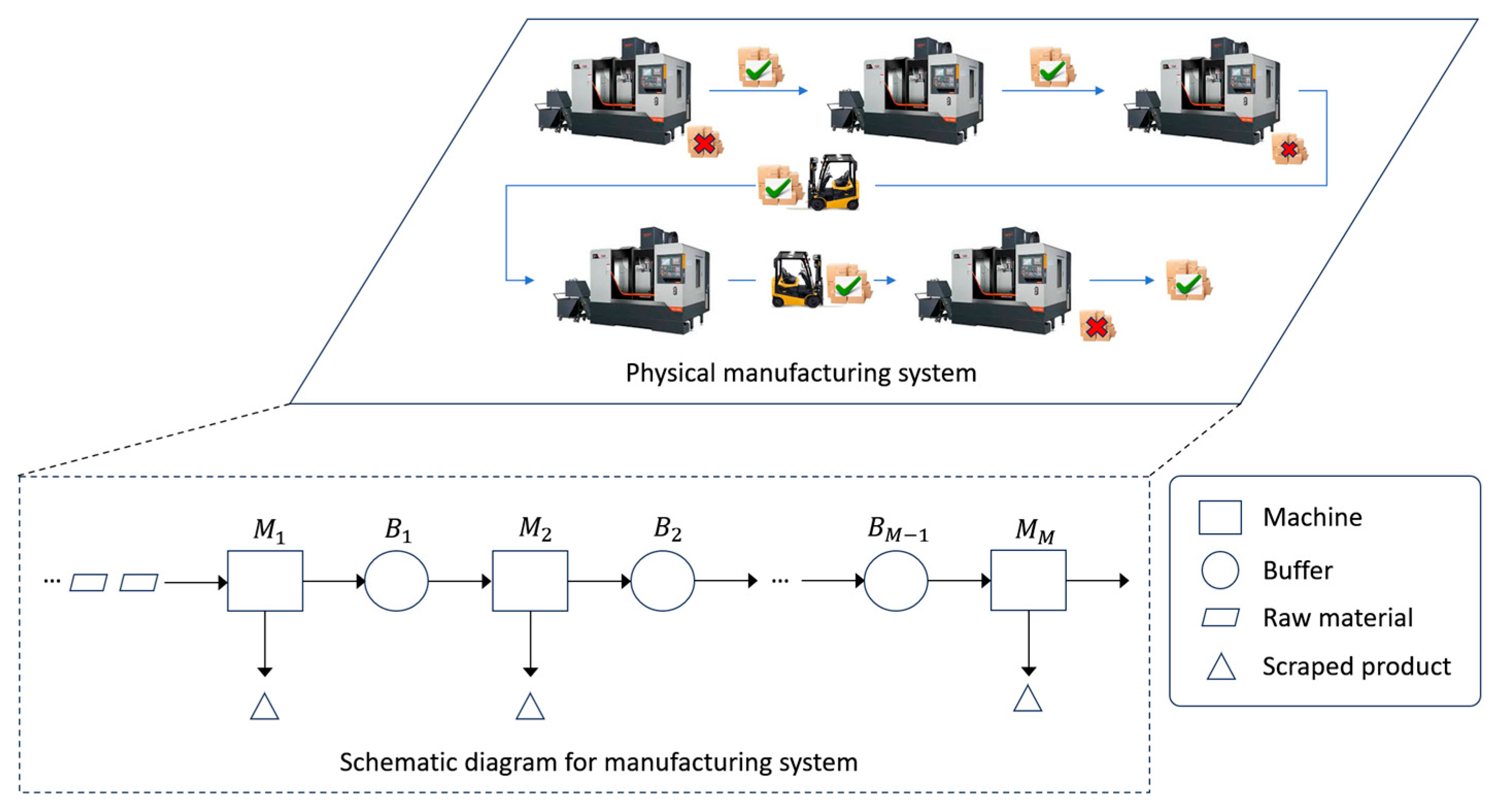
3. System Descriptions

This paper investigates a multistage manufacturing system with product quality scrap. Figure 1 shows the relationship between a physical production system and its schematic representation. The system consists of $M$ machines and $M-1$ buffers, where machines and buffers are represented by rectangles and circles, respectively. In the production process, raw materials enter the system through machine $M_1$, which produces defective products with a certain probability. These defective products are immediately scrapped. Good products are sent to buffer $B_1$, and are subsequently processed by machine $M_2$. The products then sequentially move through each subsequent buffer and machine in the system, eventually exiting as finished goods after processing by machine $M_M$. The following definitions and assumptions are adopted.

• The manufacturing system consists of $M$ machines, denoted as $M_m$ where$1\le m\le M$, and $M-1$ buffers, denoted as $B_m$ where $1\le m\le M-1$.
• All machines operate with an identical cycle time, which is the time to process a product on a machine. The timeline is discretized into time slots, each corresponding to the length of one cycle time.
• Each machine is assumed to operate under an independent geometric reliability model if there is no EC action. In each time slot, if machine $M_m$ is up, it may fail and transition to the down state with probability $p_m$, referred to as its failure probability. Conversely, if the machine $M_m$ is down, it can be restored to the up state with probability $r_m$, known as its repair probability. The state of each machine is determined at the beginning of each time slot. An operation-dependent failure mode is assumed, meaning that failures occur only when the machine is processing a part, for example, a tool breakage.
• A machine in the up state may be transitioned to the energy-saving state and can also return from the energy-saving state to up state. A machine cannot transition directly between the energy-saving state and down state. Production does not occur when a machine is either in the energy-saving state or in the down state. The state of machine $M_m$ at time $t$ is denoted by the variable ${\alpha }_m\left(t\right)\in \left\{-1, 0, 1\right\}$. Specifically, ${\alpha }_m\left(t\right)=-1$ indicates that machine $M_m$ is operating in the energy-saving state, ${\alpha }_m\left(t\right)=1$ indicates the up state, and ${\alpha }_m\left(t\right)=0$ indicates the down state.
• Machine $M_m$ yields a good product with probability $g_m$ and generates a defective product with probability $1-g_m$. Defective products are promptly scrapped, whereas good products are moved to the adjacent downstream buffer for further processing.
• Buffer $B_m$ has a finite buffer capacity, also denoted as $B_m$, where $0<B_m<\infty$. The number of products in buffer $B_m$ at time $t$ is denoted by $b_m\left(t\right)$, where $0\le b_m\left(t\right)\le B_m$. The numbers of products in the buffers are updated at the end of each time slot.
• Machine $M_m$, where $1\le m<M$, is blocked if it can produce a product but its immediate downstream buffer $B_m$ is full and the downstream machine $M_{m+1}$ is unable to produce. Machine $M_M$ is never blocked.
• Machine $M_m$, where $1<m\le M$, is starved if it can produce a product but the buffer $B_{m-1}$ is empty. Machine $M_1$ is never starved.
• When machine $M_m$ is producing a product, it consumes energy at a rate of $e_m^p$. When it is idle, either due to starvation or blockage, the energy consumption rate reduces to $e_m^i$. In energy-saving state, the consumption rate is further reduced to $e_m^e$. No energy is consumed by machine $M_m$ while it is in the down state.
• Machine $M_m$ requires a fixed warmup energy $e_m^w$ each time it transitions from the energy-saving state to up state. Transitioning from the up state to energy-saving state does not require extra energy.

Based on Assumptions (1) to (10), the research objectives investigated in this paper are as follows:

(1)

To develop analytical methods for evaluating system performance and determining the optimal EC policy for two-stage manufacturing systems with product quality scrap.

(2)

To propose an effective and computationally efficient algorithm to approximate the optimal EC policy for each machine within multistage manufacturing systems.

Detailed solutions to these objectives are presented in Section 4 and Section 5.

4. A Markov Decision Process for Two-Stage Manufacturing Systems

This section provides an analysis of a two-stage manufacturing system with product quality scrap. Based on the assumptions presented in Section 3, a discrete-time Markov decision process (MDP) is developed to determine the optimal EC policy. The objective of the MDP is to maximize the expected total discounted reward over a long time horizon. The output is an EC policy that specifies the optimal EC actions for all machines at each time slot. Formally, the MDP is characterized by the following four-tuple:

$$\left\{\mathcal{S},\mathcal{A},\mathcal{T},\mathcal{R}\right\},$$

(1)

where $\mathcal{S}$ is the system state space, $\mathcal{A}$ is the action space, $\mathcal{T}$ is the transition matrix, and $\mathcal{R}$ is the reward function. The details of state space, action space, transition probabilities, and reward function are presented in the subsequent subsections.

4.1. State and Action Spaces

In a two-stage manufacturing system, each system state comprises the machine states ${\alpha }_1\left(t\right)$ and ${\alpha }_2\left(t\right)$, as well as the buffer level $b_1\left(t\right)$ of buffer $B_1$. The system state at time $t$ is denoted as $\overrightarrow{s}\left(t\right)=\left\{b_1\left(t\right),{\alpha }_1\left(t\right),{\alpha }_2\left(t\right)\right\}$. In this way, changes in both machine conditions and buffer level are tracked and incorporated into the EC decisions. The state space $\mathcal{S}$ consists of all possible system states, i.e., $\mathcal{S}=\left\{\overrightarrow{\mathit{s}}\left(\mathit{t}\right)\right\}$.

The action space $\mathcal{A}$ comprises all feasible EC actions associated with the system state $\overrightarrow{s}\left(t\right)$. Since the states of the two machines are independent, there are two separate action sets that independently control the EC actions for each machine. The decision variable $a_m\left(\overrightarrow{s}\left(t\right)\right)=\left\{1, 0\right\}$ represents the decision for machine $M_m$ under the system state $\overrightarrow{s}\left(t\right)$. Specifically, $a_m\left(\overrightarrow{s}\left(t\right)\right)=1$ indicates that machine $M_m$ is switched to the up state at time $t$, and $a_m\left(\overrightarrow{s}\left(t\right)\right)=0$ indicates that machine $M_m$ is switched to the energy-saving state at time $t$. It is important to note that, since the system state captures the dynamics of the two-stage manufacturing system, the decision for a single machine depends not only on its own condition, but also on the buffer level and the operating state of the neighboring machine.

Let $\overrightarrow{a}\left(t\right)=\left(a_1\left(t\right),a_2\left(t\right)\right)$ represent the set of actions for the entire system, corresponding to the combined actions executed by both machines. For example, the action pair $\left(1, 0\right)$ means that machine $M_1$ is switched to up sate, and machine $M_2$ is switched to energy-saving state. The set of all possible actions is shown as:

$$\mathcal{A}=\left\{\left(1,1\right),\left(1,0\right),\left(1,0\right),\left(0,0\right)\right\}.$$

(2)

4.2. Reward Function and Transition Matrix

The production dynamics of the two-stage manufacturing system are described as:

$$\begin{array}{c}{b}_1\left(t\right)=b_1\left(t-1\right)+{\eta }_1\left(t\right)\cdot {PC}_1\left(t\right)-{PC}_2\left(t\right),\end{array}$$

(3)

where ${PC}_m\left(t\right)$ represents the number of products produced by $M_m$ at time $t$, for $m=1, 2$. The variable ${\eta }_1\left(t\right)\in \left\{0, 1\right\}$ is an indicator that reflects whether the product produced by machine $M_1$ at time $t$ meets quality standards. Specifically, ${\eta }_1\left(t\right)=1$ indicates that the product is of good quality, while ${\eta }_1\left(t\right)=0$ indicates that the product is defective.

For machine $M_2$, the value of ${PC}_2\left(t\right)$ is determined by the buffer level $b_1\left(t-1\right)$ at time $t-1$, as well as the state ${\alpha }_2\left(t\right)$ at time $t$. The expression for ${PC}_2\left(t\right)$ is given by:

$${PC}_2\left(t\right)=\min \left\{{\alpha }_2\left(t\right),b_1\left(t-1\right)\right\}.$$

(4)

For machine $M_1$, the value of ${PC}_1\left(t\right)$ is determined by the available buffer space $B_1-b_1\left(t-1\right)+P{C}_2\left(t\right)$ at time $t$ and the state ${\alpha }_1\left(t\right)$ at time $t$. The expression for ${PC}_1\left(t\right)$ is presented as:

$${PC}_1\left(t\right)=\min \left\{{\alpha }_1\left(t\right),B_1-b_1\left(t-1\right)+P{C}_2\left(t\right)\right\}.$$

(5)

Considering that every product produced by machine $M_m$ can be either good or defective, the throughput of machine $M_m$ at time $t$, which is denoted as $T{H}_m\left(t\right)$, represents the number of good products produced. $T{H}_m\left(t\right)$ is expressed as:

$${TH}_m\left(t\right)={\eta }_m\left(t\right)\cdot {PC}_m\left(t\right),m=1, 2.$$

(6)

At time $t$, the energy consumption of machine $M_m$ is estimated as:

$${EC}_m\left(t\right)=e_m+e_m^w\cdot a_m\left(t\right),m=1, 2,$$

(7)

where $e_m$ denotes the energy consumption during the production process. It is determined as:

$$e_m=\left\{\begin{array}{l}{e}_m^p,\hspace{1em}{PC}_m\left(t\right)=1,\\ e_m^i,{\alpha }_m=1 \mathrm{and} {PC}_m\left(t\right)=0,\\ e_m^e,\hspace{1em}{\alpha }_m\left(t\right)=-1,\\ 0,\hspace{1em}\hspace{1em}{\alpha }_m\left(t\right)=0.\end{array}\right.$$

The system’s energy consumption is the summation of the energy consumption of both machines, which is given by:

$$EC\left(t\right)={\sum }_{m=1}^2{EC}_m\left(t\right).$$

(8)

The reward function $r\left(\overrightarrow{s}\left(t\right),\overrightarrow{a}\left(t\right)\right)$ of MDP consists of system throughput revenue and energy consumption costs, which is calculated as:

$$r\left(\overrightarrow{s}\left(t\right),\overrightarrow{a}\left(t\right)\right)={\varphi }_{TH}\cdot T{H}_2\left(t\right)-{\varphi }_{EC}\cdot EC\left(t\right),$$

(9)

where ${\varphi }_{TH}$ is the unit benefit of throughput and ${\varphi }_{EC}$ is the unit cost of energy consumption. The impact of quality-related scrap is embedded in the revenue term. Such scalarization is commonly used in the literature, in which multiple performance indicators are integrated into a single economic metric for operational decision-making [4,24].

While the reward function focuses on throughput benefit and energy consumption cost, the framework can be extended to optimize electricity costs or greenhouse gas emissions. Such an extension would directly contribute to meeting Scope 2 emissions-reduction targets and could provide economic benefits under carbon-pricing mechanisms. For example, let $\kappa$ denote the average grid-emission factor (kg CO2-eq/kWh). The expected emission reduction over a time horizon $T$ is given by $\Delta EC·\kappa ·T$, where $\Delta EC$ represents the average power saving (kW). Specifically, $\Delta EC$ is calculated as the difference between the energy consumption rates without and with EC actions, i.e., $\Delta EC=EC{\left(t\right)}_{without EC}-EC{\left(t\right)}_{with EC}$.

To characterize the evolution of the system state, the transition rules for buffer $B_1$ are derived based on Equations (3)–(6). Given the system state $\overrightarrow{s}\left(t\right)$ and EC action $\overrightarrow{a}\left(t\right)$ at time $t$, the transition rules are determined by the throughput of the machine $M_1$ and the number of products produced by machine $M_2$. These transition rules are summarized in

Table 1. Transition rules of buffer $B_1$.

${\mathit{b}}_1\left(\mathit{t}\right)$	$\left[\mathit{T}{\mathit{H}}_1\left(\mathit{t}\right),{\mathit{P}\mathit{C}}_2\left(\mathit{t}\right)\right]$	${\mathit{b}}_1\left(\mathit{t} + 1\right)$
$0$	$T{H}_1\left(t\right)=0$	$0$
	$T{H}_1\left(t\right)=1$	1
$b_1$	$T{H}_1\left(t\right)=0$ , ${PC}_2\left(t\right)=1$	$b_1-1$
	$T{H}_1\left(t\right)=1$ ,${PC}_2\left(t\right)=1$ or $T{H}_1\left(t\right)=0$ , ${PC}_2\left(t\right)=0$	$b_1$
	$T{H}_1\left(t\right)=1$ , ${PC}_2\left(t\right)=0$	$b_1+1$
$B_1$	$T{H}_1\left(t\right)=0$ , ${PC}_2\left(t\right)=1$	$B_1-1$
	${PC}_2\left(t\right)=0$ , or $T{H}_1\left(t\right)=1$ ,${PC}_2\left(t\right)=1$	$B_1$

.

The transition matrix, which is denoted as $T_1$, includes all possible system states and their corresponding transition probabilities. Based on the assumptions, a two-stage manufacturing system has a total of $h=3^2\left(B_1+1\right)$ system states. Each system state $\overrightarrow{s}=\left\{b_1,{\alpha }_1,{\alpha }_2\right\}$ is assigned an index $\gamma$ calculated as:

$$\gamma \left(b_1,{\alpha }_1,{\alpha }_2\right)=3\left(B_1+1\right)\left({\alpha }_1+1\right)+\left(B_1+1\right)\left({\alpha }_2+1\right)+b_1+1.$$

(10)

Given the EC decision $\overrightarrow{a}\left(t\right)$, the transition matrix $T_1$ is defined as an $h\times h$-dimensional matrix, where each row corresponds to an indexed system state. Each entry in matrix $T_1$ is calculated as:

$$\begin{array}{c}{T}_1\left(\gamma \left(b_1,{\alpha }_1,{\alpha }_2\right),\gamma \left(b_1^{\prime },{\alpha }_1^{\prime },{\alpha }_2^{\prime }\right)\right)=P\left[{\overrightarrow{s}}^{\prime }|\overrightarrow{s},\overrightarrow{a}\right]\cdot {P\left[{\overrightarrow{s}}^{\prime }|\overrightarrow{s},\overrightarrow{a}\right]}^q\end{array},$$

(11)

where $P\left[{\overrightarrow{s}}^{\prime }|\overrightarrow{s},\overrightarrow{a}\right]$ denotes the transition probability due to machine state changes, and ${P\left[{\overrightarrow{s}}^{\prime }|\overrightarrow{s},\overrightarrow{a}\right]}^q$ denotes the transition probability caused by production quality scrap from machine $M_1$.

Since the states of the two machines are independent, $P\left[{\overrightarrow{s}}^{\prime }|\overrightarrow{s},\overrightarrow{a}\right]$ is obtained as the product of the transition probabilities of individual machine states:

$$\begin{array}{c}P\left[{\overrightarrow{s}}^{\prime }|\overrightarrow{s},\overrightarrow{a}\right]={\prod }_{m=1}^2{P}_m\end{array},$$

(12)

where $P_m$ is the state transition probability of machine $M_m$. It is calculated as:

$$P_m=\left\{\begin{array}{l}{p}_m, \hspace{1em}{\alpha }_m=1 \mathrm{and} {\alpha }_m^{\prime }=0,\\ 1-r_m, {\alpha }_m=1 \mathrm{and} {\alpha }_m^{\prime }=1,\\ r_m, \hspace{1em}{\alpha }_m=0 \mathrm{and} {\alpha }_m^{\prime }=1,\\ 1-p_m, {\alpha }_m=0 \mathrm{and} {\alpha }_m^{\prime }=0.\end{array}\right.$$

If there is no product quality scrap, the buffer state transition is determined by machine states. However, in the presence of product quality scrap, the buffer state transition depends not only on the machine state but also on the product quality state of machine $M_1$. Therefore, ${P\left[{\overrightarrow{s}}^{\prime }|\overrightarrow{s},\overrightarrow{a}\right]}^q$ accounts for this dependency and is calculated as:

$${P\left[{\overrightarrow{s}}^{\prime }|\overrightarrow{s},\overrightarrow{a}\right]}^q=\left\{\begin{array}{l}{g}_1, \hspace{1em}{\alpha }_m=1 \mathrm{and} {TH}_1\left(t\right)=1,\\ 1-g_1, {\alpha }_m=1 \mathrm{and} {TH}_1\left(t\right)=0,\\ 1, \mathrm{otherwise}.\end{array}\right.$$

(13)

4.3. Dynamic Programming Algorithm

An EC policy, denoted as $\pi$, determines whether the machines transition to the energy-saving state based on the current system state. The corresponding value function under policy $\pi$, denoted as $V\left(\pi ,\overrightarrow{s}\right)$, measures the expected total discounted reward over an infinite horizon starting from state $\overrightarrow{s}$. It is expressed as:

$$V\left(\pi ,\overrightarrow{s}\right)={\sum }_{t=0}^{\mathrm{\infty }}{\lambda }^t{E}_{\pi ,\overrightarrow{s}}r\left(\overrightarrow{s},\overrightarrow{a}\right),$$

(14)

where $\lambda$ is a discount factor with $0<\lambda <1$.

The optimal EC policy ${\pi }^{\ast }$ maximizes the expected total reward over an infinite horizon. It satisfies $V\left({\pi }^{\ast },\overrightarrow{s}\right)\ge V\left(\pi ,\overrightarrow{s}\right)$ for all $\pi \ne {\pi }^{\ast }$ and $\overrightarrow{s}\in \mathcal{S}$. The optimal policy can be derived by solving Bellman’s optimality equation:

$$V\left({\pi }^{\mathrm{*}},\overrightarrow{s}\right)=\underset{\overrightarrow{a}\in \mathcal{A}}{\max }\left[r\left(\overrightarrow{s},\overrightarrow{a}\right)+\lambda {\sum }_{{\overrightarrow{s}}^{\mathbf{\prime }}}P\left({\overrightarrow{s}}^{\mathbf{\prime }}|\overrightarrow{s},\overrightarrow{a}\right)V\left({\pi }^{\mathrm{*}},{\overrightarrow{s}}^{\prime }\right)\right],\forall \overrightarrow{s},{\overrightarrow{s}}^{\mathbf{\prime }}\in \mathcal{S}.$$

(15)

A dynamic programming (DP) algorithm is employed to solve the MDP for the two-stage manufacturing system. The steps of the DP algorithm are presented in Algorithm 1.

Algorithm 1: Dynamic Programming Algorithm

1.  Input: state space $\mathcal{S}$ , action space $\mathcal{A}$ , machine failure rate $p_m$ , repair rate $r_m$ and good products probability $g_m$ , buffer capacity $B_m$ , discount factor $\gamma$ , convergence threshold $ϵ$. 2.   Initialization: For all states $\overrightarrow{s}\in \mathcal{S}$, initialize value function $V\left(\overrightarrow{s}\right)=0$ 3.   For each state $\overrightarrow{s}\in \mathcal{S}$ 4.    Compute the value function       $V^{\prime }\left(\overrightarrow{s}\right)=\underset{\overrightarrow{a}\in \mathcal{A}}{\max }\left[r\left(\overrightarrow{s},\overrightarrow{a}\right)+\gamma {\sum }_{{\overrightarrow{s}}^{\prime }}P\left({\overrightarrow{s}}^{\prime }|\overrightarrow{s},\overrightarrow{a}\right)V\left({\overrightarrow{s}}^{\prime }\right)\right]$ 5.    If $\max \left|V^{\prime }\left(\overrightarrow{s}\right)-V\left(\overrightarrow{s}\right)\right|<ϵ$ 6.       Stop 7.    End If 8.    Update the value function $V\left(\overrightarrow{s}\right)=V^{\prime }\left(\overrightarrow{s}\right)$ 9.   End For 10.    Compute the optimal policy       ${\pi }^{\ast }\left(\overrightarrow{s}\right)=\arg \underset{\overrightarrow{a}\in \mathcal{A}}{\max }\left[r\left(\overrightarrow{s},\overrightarrow{a}\right)+\gamma {\sum }_{{\overrightarrow{s}}^{\prime }}P\left({\overrightarrow{s}}^{\prime }|\overrightarrow{s},\overrightarrow{a}\right)V\left({\overrightarrow{s}}^{\prime }\right)\right]$ 11. Output: Optimal EC policy ${\pi }^{\ast }$

Algorithm 1 employs classical value iteration to compute the optimal EC policy for the established MDP. When given system parameters, it constructs the one-step reward function and transition probability matrix, then iteratively updates the value function. Starting from $V\left(\overrightarrow{s}\right)=0$ for all $\overrightarrow{s}\in \mathcal{S}$, the algorithm repeatedly sweeps through each state, updating $V\left(\overrightarrow{s}\right)$ using Equation (15) until the maximum change $\left|V^{\prime }\left(\overrightarrow{s}\right)-V\left(\overrightarrow{s}\right)\right|$ across all states falls below convergence threshold $ϵ$. The optimal EC policy ${\pi }^{\ast }\left(\overrightarrow{s}\right)$ is then derived by selecting the action that maximizes the expected reward in each state. Algorithm 1 serves as the foundation for the proposed EC method in multistage manufacturing systems. The key idea is to decompose the multistage system into a set of two-stage subsystems. For each two-stage subsystem, Algorithm 1 is applied to derive the corresponding EC policy. This idea enables the scalable and computationally efficient control framework across complex manufacturing systems.

5. An Aggregation Procedure for Multistage Manufacturing Systems

For multistage manufacturing systems, directly modeling the system by enumerating all possible states presents significant challenges. As the number of stages increases, the state and action spaces expand exponentially, rendering the direct application of the DP algorithm impractical. To address this challenge, an aggregation procedure is developed to simplify the state and action spaces while retaining the critical system dynamics. In the aggregation procedure, multistage manufacturing systems are decomposed into two-stage building blocks. First, the proposed MDP is used to derive the optimal EC policy for each two-stage building block. Then, each block is aggregated into a virtual machine, which is subsequently combined with its immediate downstream buffer and machine to form a new two-stage building block. This iterative process continues until all machines are incorporated.

5.1. State Aggregation

To facilitate the aggregation procedure, state aggregation for a two-stage building block is applied. The fundamental concept behind state aggregation is to represent the system’s performance using a single up state and a single down state, thereby substituting the original complex model with a simplified abstraction. State aggregation is feasible since, after the EC policies are established, the state transition trajectories are set, and the associated probabilities are completely specified. Consequently, through state aggregation, a geometric reliability model can be efficiently utilized to describe the behavior of each aggregated block [25].

For the building block composed of machines $M_1$ and $M_2$, and the intermediate buffer $B_1$, the system dynamics can be modeled as a discrete-time Markov chain under a given EC policy ${\pi }^{a_1,a_2}$. The corresponding state transition matrix $T_1$ is derived from Equation (11). Let the steady-state probability distribution be denoted as $P_{sys}=\left[P\left({\overrightarrow{s}}_1\right),\dots ,P\left({\overrightarrow{s}}_h\right)\right]$. The steady-state distribution satisfies the global balance equations:

$$P_{sys}=T_1\cdot P_{sys}.$$

(16)

Following reference [26], the steady-state distribution $P_{sys}$ is obtained by solving Equation (16).

After state aggregation, a virtual machine ${\overline{M}}_2$ is introduced to represent the behavior of the two-stage building block. ${\overline{\alpha }}_2=\left\{1,0\right\}$ denotes the states of machine ${\overline{M}}_2$. Specifically, ${\overline{\alpha }}_2=1$ represents the up state and ${\overline{\alpha }}_2=0$ represents the down state. Let ${\overline{r}}_2$ denote the repair rate and ${\overline{p}}_2$ denote the failure rate. Then, the state transition matrix ${\overline{T}}_2$ of virtual machine ${\overline{M}}_2$ is expressed as:

$${\overline{T}}_2=\left(\begin{array}{cc}1-{\overline{p}}_2& {\overline{p}}_2\\ {\overline{r}}_2& 1-{\overline{r}}_2\end{array}\right).$$

(17)

Given a two-stage manufacturing system satisfying Assumptions (1) to (10), the repair rate ${\overline{r}}_2$ and failure rate ${\overline{p}}_2$ of virtual machine ${\overline{M}}_2$, and the blocking probability $B{L}_1$ of the upstream machine $M_1$ can be calculated as:

$$\begin{array}{l}{\overline{r}}_2={\displaystyle \frac{{\sum }_{{\overrightarrow{s}}^{\prime }\in {\xi }_2}{\sum }_{\overrightarrow{s}\in {\xi }_1}\hspace{1em}P\left(\overrightarrow{s}\right)\cdot P\left({\overrightarrow{s}}^{\prime }|\overrightarrow{s},\overrightarrow{a}\right)}{{\sum }_{\overrightarrow{s}\in {\xi }_1}\hspace{1em}P\left(\overrightarrow{s}\right)}},\\ {\overline{p}}_2={\displaystyle \frac{{\sum }_{{\overrightarrow{s}}^{\prime }\in {\xi }_1}{\sum }_{\overrightarrow{s}\in {\xi }_2}\hspace{1em}P\left(\overrightarrow{s}\right)\cdot P\left({\overrightarrow{s}}^{\prime }|\overrightarrow{s},\overrightarrow{a}\right)}{{\sum }_{\overrightarrow{s}\in {\xi }_2}\hspace{1em}P\left(\overrightarrow{s}\right)}},\\ B{L}_1=P\left({\xi }_3\right), \end{array}$$

(18)

where the state subsets ${\xi }_1$, ${\xi }_2$, and ${\xi }_3$ are defined as:

$$\begin{array}{l}{\xi }_1=\left\{\left(b_1,{\alpha }_1,{\alpha }_2\right)|{\alpha }_2\ne 1 \mathrm{o}\mathrm{r} b_1=0\right\},\\ {\xi }_2=\left\{\left(b_1,{\alpha }_1,{\alpha }_2\right)|{\alpha }_2=1 \mathrm{a}\mathrm{n}\mathrm{d} b_1\ne 0\right\},\\ {\xi }_3=\left\{\left(b_1,{\alpha }_1,{\alpha }_2\right)|{\alpha }_1=1,{\alpha }_2\ne 1 \mathrm{a}\mathrm{n}\mathrm{d} b_1=B_1\right\}.\end{array}$$

5.2. Initial Policies Generation

Following state aggregation, the virtual machine is then combined with its immediate downstream buffer and machine to form a new two-stage building block. This iterative process facilitates the derivation of the optimal EC policies for adjacent machines within the multistage manufacturing system. Specifically, the virtual machine ${\overline{M}}_2$ is combined with buffer $B_2$ and machine $M_3$. The optimal EC policy for machine $M_3$, which is denoted as ${\pi }^{a_3}$, is then derived. For machine $M_m$, where $m\ge 3$, given the EC policy ${\pi }^{a_m}$, the transition matrix ${\overline{T}}_m$ of the virtual machine ${\overline{M}}_m$ is derived using the matrix ${\overline{T}}_{m-1}$ from the previous virtual machine ${\overline{M}}_{m-1}$, the quality parameter $g_{m-1}$ from machine $M_{m-1}$, parameters $p_m$, $r_m$, and $g_m$ from machine $M_m$, and the buffer capacity $B_{m-1}$. Additionally, the blocking probability ${BL}_{m-1}$ of the machine $M_{m-1}$ is also calculated as part of the iterative procedure.

Using the iterative process described above, two generators $G_1^{\overline{T}}$ and $G_2^{\overline{T}}$ are defined to represent the construction of ${\overline{T}}_m$, for $2\le m\le M-1$. These generators are defined as:

$$\left\{\begin{array}{c}{\overline{T}}_2=G_1^{\overline{T}}\left({\pi }^{a_1,a_2},T_1\right),\hspace{1em}m=1,\\ \left[{\overline{T}}_{m+1},{BL}_m\right]=G_2^{\overline{T}}\left({\pi }^{a_{m+1}},{\overline{T}}_m\right), 2\le m\le M-2.\end{array}\right.$$

(19)

Additionally, two generators $G_1^{\pi }$ and $G_2^{\pi }$ are defined to generate the EC policies. They are expressed as:

$$\left\{\begin{array}{l}{\pi }^{a_1,a_2}=G_1^{\pi }\left(T_1\right),\hspace{1em}m=1,\\ {\pi }^{a_{m+1}}=G_2^{\pi }\left(T_m\right), 2\le m\le M-1.\end{array}\right.$$

(20)

By combining Equations (19) and (20), the procedure for generating initial EC policies is summarized in Algorithm 2.

Algorithm 2: Generating initial EC policies

1.  Input: machine failure rate $p_m$ , repair rate $r_m$ and good products probability $g_m$ , buffer capacity $B_m$ . 2.  For $m=2:M$ 3.    If $m=2$ , 4.        $\begin{array}{c}{\pi }^{a_1,a_2}=G_1^{\pi }\left(T_1\right),\\ \hspace{1em}\hspace{1em}\hspace{1em} {\overline{T}}_2=G_1^{\overline{T}}\left({\pi }^{a_1,a_2},T_1\right).\end{array}$ 5.    If $2\le m\le M-2$ , 6.      $\begin{array}{c}{\pi }^{a_{m+1}}=G_2^{\pi }\left(T_m\right),\\ \left[{\overline{T}}_{m+1},{BL}_m\right]=G_2^{\overline{T}}\left({\pi }^{a_{m+1}},{\overline{T}}_m\right).\end{array}$ 7.    If $m=M-1$ , 8.         ${\pi }^{a_M}=G_2^{\pi }\left(T_{M-1}\right)$ . 9.  End For 10.   Output: initial EC policies ${\pi }^{a_1,a_2}$ , ${\pi }^{a_{m+1}},2\le m\le M-2$ .

5.3. Aggregation Procedure

Algorithm 2 does not consider the blocking effects of downstream machines on upstream machines. Consequently, the initial EC policies derived through this algorithm do not fully represent the optimal EC policy. To address this limitation, machine failure and repair rates are updated by incorporating blocking probabilities.

When machine $M_m$ is blocked, it is in the up state but is unable to produce products. This condition indicates that the operating time of machine $M_m$ is reduced compared to a scenario in which blockage is absent. It is well known that blockage impacts the efficiency of machine $M_m$, which is calculated as $e_m={\displaystyle \frac{R_m}{P_m+R_m}}$. When incorporating the effects of blockage, the actual efficiency of machine $M_m$ is given by $e_m^{\prime }={\displaystyle \frac{R_m\left(1-{BL}_m\right)}{P_m+R_m}}$. From the numerator of $e_m^{\prime }$, it follows that the effective repair rate should be adjusted to $R_m\left(1-{BL}_m\right)$. Therefore, the updated formulas for the failure and repair rates are expressed as:

$$\begin{array}{c}{P}_m^{\prime }=P_m+R_m\cdot {BL}_m,\\ R_m^{\prime }=R_m-R_m\cdot {BL}_m,\end{array}2\le m\le M-1,$$

(21)

where $P_m^{\prime }$ and $R_m^{\prime }$ are the updated failure and repair rates, respectively. Note that machine $M_M$ cannot be blocked and machine $M_1$ does not undergo state aggregation. Consequently, these two machines do not require parameter updates.

Adjustments to the failure and repair rates further result in corresponding changes to the transition matrix Tm of the building block. To describe the generation of the modified transition matrix, a generator $G^{T^{\prime }}$ is defined as:

$$T_{m-1}^{\prime }=G^{T^{\prime }}\left(T_{m-1},{BL}_m\right), 2\le m\le M-1.$$

(22)

By following the updating procedure, the influence of blockages can be integrated into the development of the EC policy for each machine. However, the initial blocking probabilities are computed using the initial EC policies, under the assumption that the second machine in each two-stage building block does not experience any blocking. As the blocking probabilities change, the EC policies also need to be updated. To address this interdependence, an aggregation procedure is introduced to simultaneously update both the EC policies and the blocking probabilities. The details of this procedure are summarized in Algorithm 3.

Algorithm 3: Aggregation procedure

1.  Input: machine failure rate $p_m$ , repair rate $r_m$ and good products probability $g_m$ , buffer capacity $B_m$ , convergence threshold $ϵ$ , maximum iteration count $I$ . 2.  Initialization: ${BL}_m\left(0\right)=0, 2\le m\le M-1$ , ${BL}_M\left(i\right)=0, 0\le i\le I$ . 3.  For $i=1:I$ 4.   For $m=1:M-1$ 5.      If $m=1$ , 6.     $\begin{array}{c}\hspace{1em}\hspace{1em}\hspace{1em}\hspace{1em} T_1^{\prime }\left(i\right)=G^{T\prime }\left(T_1,{BL}_2\left(i-1\right)\right),\\ {\pi }^{a_1,a_2}\left(i\right)=G_1^{\pi }\left(T_1^{\prime }\left(i\right)\right),\\ \hspace{1em}\hspace{1em}\hspace{1em}\hspace{1em} {\overline{T}}_2\left(i\right)=G_1^{\overline{T}}\left({\pi }^{a_1,a_2}\left(i\right),T_1^{\prime }\left(i\right)\right).\end{array}$ 7.      If $2\le m\le M-2$ , 8.     $\begin{array}{c}\hspace{1em}\hspace{1em}\hspace{1em}\hspace{1em} T_m^{\prime }\left(i\right)=G^{T\prime }\left(T_m,{BL}_{m+1}\left(i-1\right)\right),\\ {\pi }^{a_{m+1}}\left(i\right)=G_2^{\pi }\left(T_m^{\prime }\left(i\right)\right),\\ \left[{\overline{T}}_{m+1}\left(i\right),{BL}_m\left(i\right)\right]=G_2^{\overline{T}}\left({\pi }^{a_{m+1}}\left(i\right),T_m^{\prime }\left(i\right)\right).\end{array}$ 9.      If $m=M-1$ , 10.           ${\pi }^{a_M}\left(i\right)=G_2^{\pi }\left(T_{M-1}^{\prime }\left(i\right)\right)$ . 11.   End For 12.   If $\left|{BL}_m\left(i\right)-{BL}_m\left(i-1\right)\right|\le ϵ$ , $\forall 2\le m\le M-1$ 13.      Break 14.    End If 15.   End For 16.  Output: EC policies ${\pi }^{a_1,a_2}$ , ${\pi }^{a_m},3\le m\le M$ .

The derived EC policies can be applied as a lightweight lookup table and deployed within a microservice integrated into the plant’s decision support system. Sensors and PLCs capture real-time data on machine states, buffer levels, and product quality. The microservice maps each state vector to an optimal EC action within milliseconds and transmits the command back to the machine controller via standard industrial protocols. As the policy is offline, the online computational overhead is minimal, enabling an end-to-end response time within industrial cycle time constraints. Additionally, the system can expose an interface that supports real-time policy updates, allowing managers to replace the table in response to changes in product mix or electricity pricing, thereby maintaining both operational responsiveness and near-optimal control performance. In summary, the architecture turns ubiquitous shop-floor sensing and modern edge-microservice technology into a low-latency, production control layer that is fully aligned with current Industry 4.0 practice.

6. Numerical Experiments

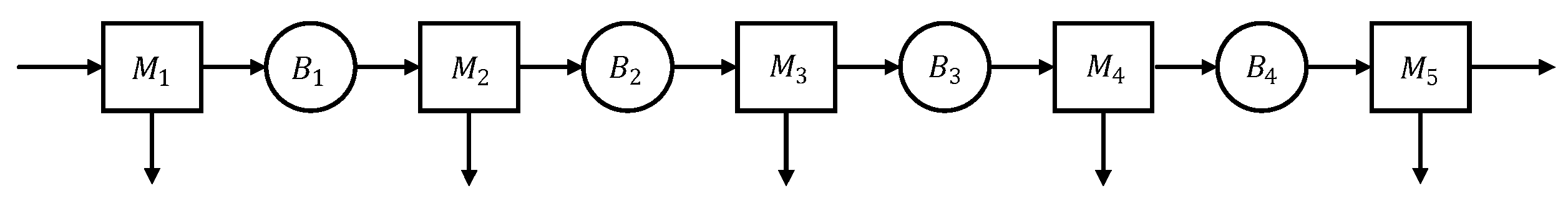
6.1. Illustrative Example

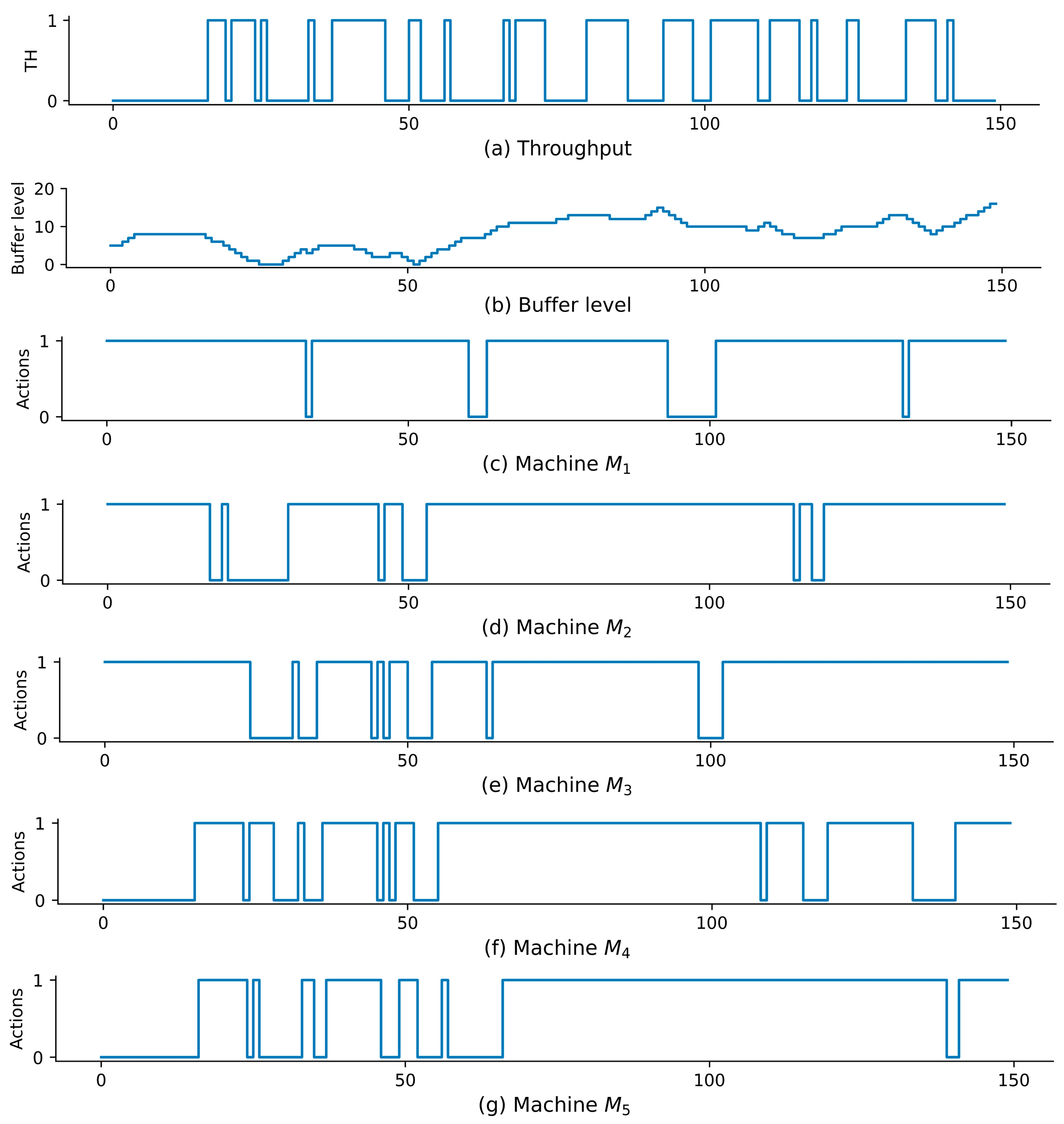
This section considers a five-stage manufacturing system, which is shown in Figure 2. The related parameters are provided in

Table 2. Related parameters of the manufacturing system.

Station	${\mathit{M}}_1$	${\mathit{M}}_2$	${\mathit{M}}_3$	${\mathit{M}}_4$	${\mathit{M}}_5$
$p_m$	0.10	0.08	0.12	0.09	0.10
$r_m$	0.30	0.25	0.27	0.29	0.30
$g_m$	0.95	0.98	0.95	0.97	0.96
$e_m^p$	15.5	14.0	15.0	14.5	15.0
$e_m^i$	12.0	11.5	12.0	11.5	12.0
$e_m^e$	0.5	0.4	0.6	0.5	0.6
$e_m^w$	5.0	5.5	5.0	5.5	5.0
Buffer	$B_1$	$B_2$	$B_3$	$B_4$
$B_m$	3	5	4	5

. The cost per unit of energy consumption is set at ${\varphi }_{EC}=0.1 \mathrm{\$}/\mathrm{k}\mathrm{W}\mathrm{h}$, while the benefit per unit of throughput is ${\varphi }_{TH}=50 \mathrm{\$}/\mathrm{k}\mathrm{W}\mathrm{h}$. The numerical experiments are performed using Python 3.9 on a Lenovo (Hong Kong, China) computer featuring an Intel(R) Core(TM) i5-8250U CPU processor (1.60–1.80 GHz), and 16 GB of RAM. According to the values of $g_m$ provided in Table 2, the scrap rates for the five machines are 0.05, 0.02, 0.05, 0.03, and 0.04, respectively.

Using the proposed dynamic EC method, the convergence threshold $ϵ$ is set to ${10}^{-6}$, and the aggregation procedure successfully converges. Figure 3 presents the updated blocking probabilities for machines $M_2$ to $M_4$. At the beginning of the aggregation procedure, blockage is not considered, and all machines are initialized with zero blocking probability. In iteration 1, these probabilities are calculated and used to update the initial policies. The blocking probabilities of machine $M_2$ in iterations 1 and 2 are 0.0618 and 0.0622, respectively. The probability is further updated in iterations 3 to 6 and stabilizes in subsequent iterations. As shown in Figure 3, the aggregation procedure generally converges in no more than seven iterations.

Under the obtained EC policies, the manufacturing system is simulated with a warm-up period of 1000 time steps, followed by an operational period of 10,000 time steps. To validate the effectiveness of dynamic EC method, the baseline scenario is created for comparison by applying the always-on policy, in which the machines are never switched to the energy-saving state. For ease of discussion, the baseline scenario is referred to as the BL scenario. The EC policy obtained by the dynamic EC method is denoted as the DEC policy. It is compared with two well-established EC methods, i.e., station-level EC (SEC) policy, upstream-buffer EC (UEC) policy [27], and energy saving opportunity window (ESOW) policy [28]. In the SEC policy, the energy consumption rates of the two machines with the highest consumption are decreased by 15%. In the UEC policy, machine $M_m,1\le m\le M$ transitions to the energy-saving state when buffer $B_{m-1}$ is empty and returns to the up state if the buffer level in $B_{m-1}$ reaches the threshold $N_{up}$. An exhaustive search method is utilized to identify the optimal threshold values for the UEC policy. ESOW policy is a periodical control method, where each control period has a constant length $d_e$. At the beginning of each control period, each machine $M_m$ in the selected machine set $\left\{M_m\right\}$ is switched to energy-saving mode for a time duration of $O{W}_m=\min \left\{{\sum }_{i=1}^{m-1}{b}_i\left(t\right),{\sum }_{i=m}^{M-1}{B}_i-b_i\left(t\right),d_e\right\}$. The selected machine set $\left\{M_m\right\}$ and control period $d_e$ are determined by simulation.

The comparison results of four policies and BL are presented in

Table 3. Comparison results of four policies and BL.

	Throughput (Parts)	Energy Consumption Cost ($)
DEC	4797	44,844.7
SEC	4795	50,307.7
UEC	4712	48,077.1
ESOW	4703	47,086.3
BL	4656	51,874.3

. The results indicate that these four policies can improve system energy efficiency compared to BL. The proposed DEC policy outperforms the other three methods, i.e., the SEC policy, the UEC policy and ESOW policy. Specifically, compared with BL, the DEC policy reduces energy consumption costs by 13.55% and improves throughput by 3.02%. The SEC policy results in the smallest energy consumption reduction of 1.52% and has almost the same throughput with BL. The UEC policy achieves a 7.32% energy consumption reduction but brings a modest 1.20% throughput improvement, while the ESOW policy reduces energy consumption by 9.23% with only a 1.01% improvement in throughput.

To analyze the characteristics of the DEC policy, a time interval spanning 150 time steps is chosen at random. Figure 4 shows the trajectories of throughput, buffer levels, and machine EC actions of the manufacturing system under the DEC policy. The results indicate that the DEC policy effectively captures EC opportunities. The results can be interpreted as follows:

(1)

When the buffer level is low, downstream machines are more likely to perform EC actions, while upstream machines tend to remain in the up state. For example, after the 20th time step, the buffer level continues to decrease, machine $M_1$ remains in the up state to replenish parts, whereas downstream machines are more frequently switched to the energy-saving state to avoid starvation.

(2)

When the buffer level is high, upstream machines have the opportunity to perform EC actions. For example, after the 90th time step, as the buffer level increases, machine $M_1$ is switched to the energy-saving state, while downstream machines remain in the up state.

6.2. Effectiveness Analysis

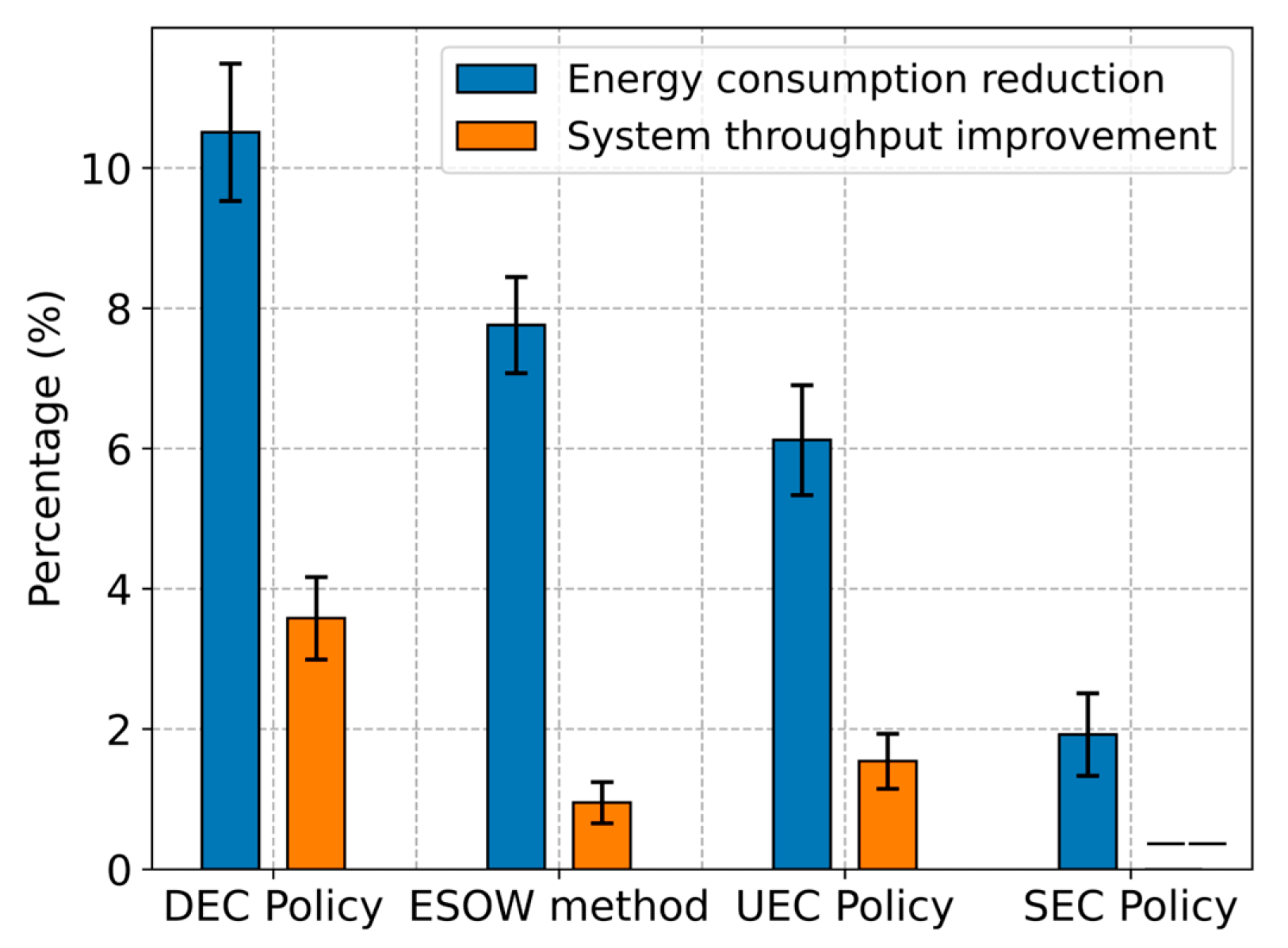
To further verify the effectiveness of the dynamic EC method, 1000 manufacturing systems are created by varying parameters, including the machine number, machine parameters (e.g., failure rates, repair rates, and good product probabilities), buffer capacities, and cost parameters. These parameters are randomly sampled from

Table 4. Production related parameters.

Parameters	Sets
Machine number	$M\in \left\{3, 6, 8, 10, 12\right\}$
Failure rate	$p_m\in \left[0.01, 0.10\right]$
Repair rate	$r_m\in \left[0.10, 0.40\right]$
Good products probability	$g_m\in \left[0.90, 0.99\right]$
Energy consumption rate	$e_m^p\in \left\{15, 30, 35\right\}$ , $e_m^e\in \left\{0.1, 0.15, 0.12\right\}\cdot e_m^p$ $e_m^i\in \left\{0.6, 0.7, 0.8\right\}\cdot e_m^p$ , $e_m^w\in \left\{5, 6, 7\right\}$
Buffer capacity	$B_m\in \left\{5, 10, 15\right\}$
Throughput benefit	${\varphi }_{TH}\in \left\{50, 100, 150\right\}$
Energy consumption cost	${\varphi }_{EC}\in \left\{0.05, 0.1, 0.15\right\}$

. In this section, the good products probability is determined within the range $\left[0.90, 0.99\right]$, which means the scrap rate is between 0.01 and 0.10. These values are representative of many real-world industrial settings. For example, typical scrap rates in Surface-Mount Technology (SMT) lines range from 5% to 10% [29], while scrap rates in silicon wafer fabrication processes are generally between 3% and 5% [30].

DEC policy is also compared with the SEC policy, UEC policy, and ESOW policy. Each manufacturing system is simulated for 10,000 time steps under all three policies and BL. The variables $EC$ and $TH$ represent the energy consumption cost and system throughput under each EC policy, respectively, while the variables $\widehat{EC}$ and $\widehat{TH}$ denote those under the BL scenario. The differences in energy consumption cost and system throughput between the BL and the EC policies, quantified by ${\delta }_{EC}$ and ${\delta }_{TH}$, are calculated as follows:

$${\delta }_{EC}=\left|{\displaystyle \frac{EC-\widehat{EC}}{\widehat{EC}}}\right|\cdot 100\%, {\delta }_{TH}=\left|{\displaystyle \frac{TH-\widehat{TH}}{\widehat{TH}}}\right|\cdot 100\%.$$

(23)

Figure 5 presents the average percentage reductions in energy consumption costs and improvements in system throughput achieved by the three policies compared to BL. Error bars represent the 95% confidence intervals of each value. The results show that the DEC policy has the most significant impact on improving system energy efficiency. The DEC policy achieves the greatest energy consumption reduction and system throughput improvement, which are 10.51% and 3.58%, respectively. The SEC policy results in the smallest energy consumption reduction of 1.92%. The UEC policy achieves a 6.12% energy consumption reduction but only brings a 1.54% system throughput improvement, which is about 2% lower than that of the DEC policy. The ESOW policy has an 8.76% energy consumption reduction but brings only 0.95% system throughput improvement. Based on the results, it can be concluded as follows:

(1)

The DEC policy outperforms all these three methods, i.e., the SEC policy, the UEC policy, and ESOW method, primarily due to its ability to identify energy-saving opportunities by comprehensively analyzing the interrelationships among production, energy consumption, and quality within manufacturing systems.

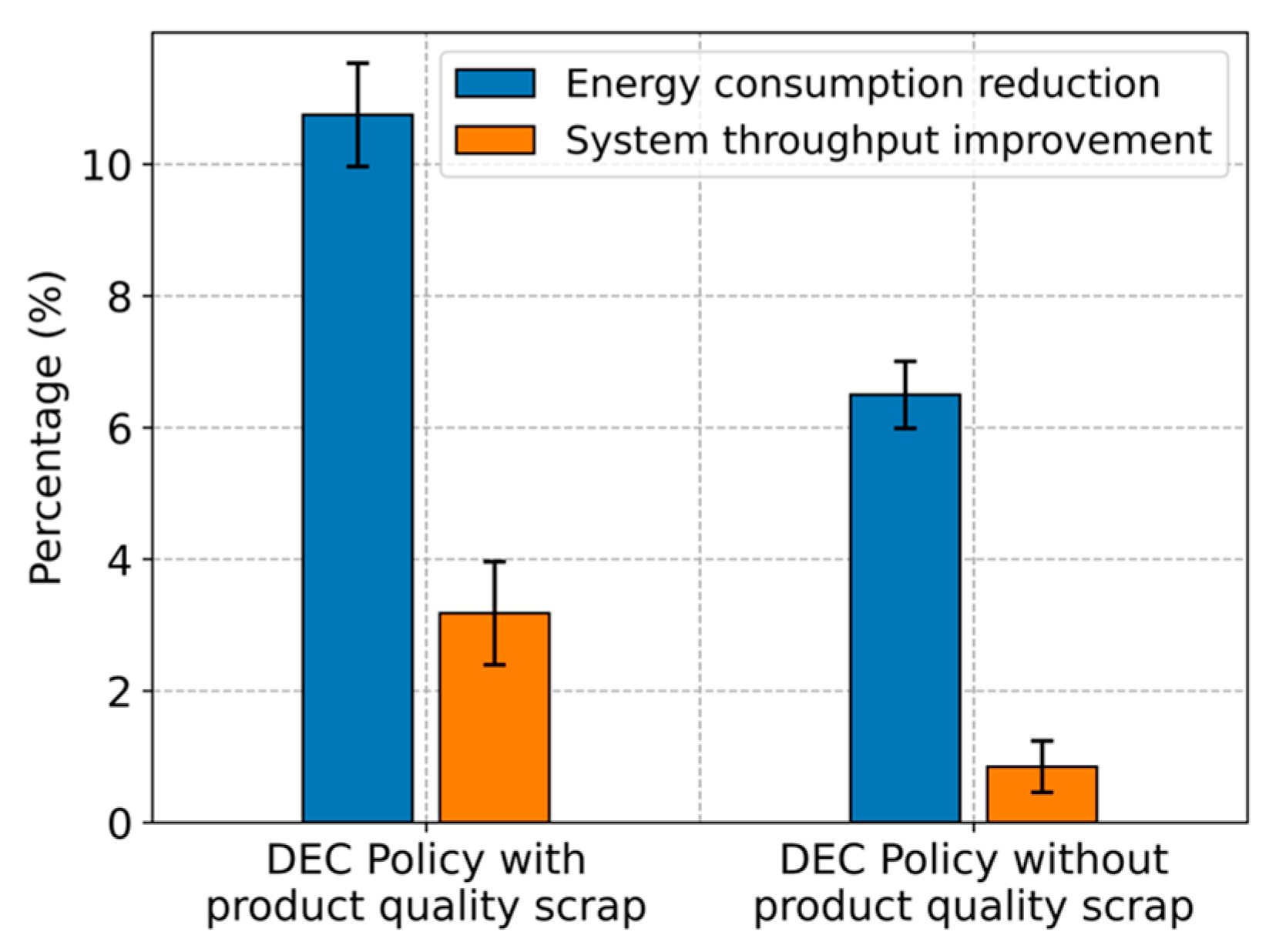
(2)

The DEC policy significantly reduces energy consumption costs and slightly improves system throughput. This performance can be attributed to the policy’s ability to utilize machine idle periods for EC. By switching machines to the energy-saving state, the DEC policy indirectly reduces the likelihood of machines producing defective products, thereby improving throughput.

6.3. Comparative Analysis

In this section, the effectiveness of the dynamic EC method is further evaluated by comparing the performance of the DEC policies obtained under two conditions: one that incorporates product quality scrap, and one that does not. This comparison aims to demonstrate the impact of incorporating product quality scrap on the effectiveness of the EC method. To conduct the comparative analysis, an additional 1000 manufacturing systems are randomly generated utilizing the parameters shown in Table 4.

The aggregation procedure is employed to derive two types of DEC policies, i.e., the DEC policies with and without product quality scrap, for each manufacturing system. Under the two derived DEC policies, each manufacturing system is simulated for 10,000 time steps. The differences in energy consumption cost and system throughput between the BL and the two DEC policies are calculated using Equation (23).

Figure 6 presents the average energy consumption reduction and average system throughput improvement of the DEC policies in scenarios with and without product quality scrap. Error bars represent the 95% confidence intervals of each value. The results show that both DEC policies achieve considerable improvements in energy efficiency compared with BL. However, the DEC policy with product quality scrap outperforms the DEC policy without product quality scrap in both energy savings and production performance. The DEC policy with product quality scrap achieves 4.25% greater energy consumption reduction and 2.33% higher system throughput improvement than the DEC policy without product quality scrap. These findings highlight the importance of integrating production quality into EC to reduce energy consumption while maintaining production performance in manufacturing systems.

7. Conclusions and Future Work

This paper investigates a dynamic energy-saving control (EC) method for multistage manufacturing systems with product quality scrap. Specifically, for two-stage manufacturing systems, the EC problem is formulated as a Markov decision process (MDP) to derive the optimal EC policy that balances throughput revenue and energy consumption costs. To overcome the curse of dimensionality in multistage manufacturing systems, an aggregation procedure that decomposes the system into two-stage building blocks is introduced to approximate the optimal EC policy for individual machines. Computational results indicate that the proposed dynamic EC method achieves substantial improvements in system energy efficiency. Furthermore, the results emphasize the importance of integrating product quality scrap into EC decision-making to further enhance system-level energy savings and throughput performance. In summary, the proposed method provides manufacturers with a practical and cost-effective tool for improving energy efficiency without compromising production performance, thereby supporting sustainable operations in complex manufacturing environments.

Although the proposed dynamic EC method achieves near-optimal policies with reasonable computational efficiency, the current model relies on several simplifying assumptions: (i) perfect observability of system states, (ii) stationary failure rates, and (iii) fixed scrap rates. These assumptions may not persist in practical shop-floor environments. In addition, the derived policy is offline and does not adapt to real-time changes in system parameters. Future work will focus on integrating deep reinforcement learning methods to enable online policy learning from streaming production data.

Another promising direction is the extension of the proposed framework to a multi-objective MDP. Future work could develop efficient $\epsilon$-constraint or weighted-sum sweep methods to approximate the Pareto set. By visualizing the trade-off frontier between energy consumption and system throughput under varying preference scenarios, decision-makers can identify control policies that align with specific strategic priorities, such as carbon-neutral operations or throughput maximization.

References

1. Nota, G.; Nota, F.D.; Peluso, D.; Lazo, A.T. Energy Efficiency in Industry 4.0: The Case of Batch Production Processes. Sustainability 2020, 12, 6631. [Google Scholar] [CrossRef]
2. Jauhari, W.A.; Pujawan, I.N.; Suef, M.; Govindan, K. Low Carbon Inventory Model for Vendor–buyer System with Hybrid Production and Adjustable Production Rate under Stochastic Demand. Appl. Math. Model. 2022, 108, 840–868. [Google Scholar] [CrossRef]
3. Ardolino, M.; Bacchetti, A.; Dolgui, A.; Franchini, G.; Ivanov, D.; Nair, A. The Impacts of Digital Technologies on Coping with the COVID-19 Pandemic in the Manufacturing Industry: A Systematic Literature Review. Int. J. Prod. Res. 2024, 62, 1953–1976. [Google Scholar] [CrossRef]
4. Li, Y.; Cui, P.-H.; Wang, J.-Q.; Chang, Q. Energy-Saving Control in Multistage Production Systems Using a State-Based Method. IEEE Trans. Autom. Sci. Eng. 2022, 19, 3324–3337. [Google Scholar] [CrossRef]
5. Brundage, M.P.; Chang, Q.; Zou, J.; Li, Y.; Arinez, J.; Xiao, G. Energy Economics in the Manufacturing Industry: A Return on Investment Strategy. Energy 2015, 93, 1426–1435. [Google Scholar] [CrossRef]
6. Wessel, J.; Turetskyy, A.; Cerdas, F.; Herrmann, C. Integrated Material-Energy-Quality Assessment for Lithium-Ion Battery Cell Manufacturing. Procedia CIRP 2021, 98, 388–393. [Google Scholar] [CrossRef]
7. Sahoo, S.; Lo, C.-Y. Smart Manufacturing Powered by Recent Technological Advancements: A Review. J. Manuf. Syst. 2022, 64, 236–250. [Google Scholar] [CrossRef]
8. Phuyal, S.; Bista, D.; Bista, R. Challenges, Opportunities and Future Directions of Smart Manufacturing: A State of Art Review. Sustain. Futures 2020, 2, 100023. [Google Scholar] [CrossRef]
9. Barenji, A.V.; Liu, X.; Guo, H.; Li, Z. A Digital Twin-Driven Approach towards Smart Manufacturing: Reduced Energy Consumption for a Robotic Cell. Int. J. Comput. Integr. Manuf. 2021, 34, 844–859. [Google Scholar] [CrossRef]
10. Cañas, H.; Mula, J.; Campuzano-Bolarín, F.; Poler, R. A Conceptual Framework for Smart Production Planning and Control in Industry 4.0. Comput. Ind. Eng. 2022, 173, 108659. [Google Scholar] [CrossRef]
11. Jiang, P.; Wang, Z.; Li, X.; Wang, X.V.; Yang, B.; Zheng, J. Energy Consumption Prediction and Optimization of Industrial Robots Based on LSTM. J. Manuf. Syst. 2023, 70, 137–148. [Google Scholar] [CrossRef]
12. El Abdelaoui, F.Z.; Jabri, A.; El Barkany, A. Optimization Techniques for Energy Efficiency in Machining Processes—A Review. Int. J. Adv. Manuf. Technol. 2023, 125, 2967–3001. [Google Scholar] [CrossRef]
13. Nouiri, M.; Bekrar, A.; Trentesaux, D. An Energy-Efficient Scheduling and Rescheduling Method for Production and Logistics Systems†. Int. J. Prod. Res. 2020, 58, 3263–3283. [Google Scholar] [CrossRef]
14. Karimi, S.; Kwon, S.; Ning, F. Energy-Aware Production Scheduling for Additive Manufacturing. J. Clean. Prod. 2021, 278, 123183. [Google Scholar] [CrossRef]
15. Tan, B.; Karabağ, O.; Khayyati, S. Production and Energy Mode Control of a Production-Inventory System. Eur. J. Oper. Res. 2023, 308, 1176–1187. [Google Scholar] [CrossRef]
16. Loffredo, A.; May, M.C.; Matta, A.; Lanza, G. Reinforcement Learning for Sustainability Enhancement of Production Lines. J. Intell. Manuf. 2024, 35, 3775–3791. [Google Scholar] [CrossRef]
17. Loffredo, A.; Frigerio, N.; Lanzarone, E.; Matta, A. Energy-Efficient Control in Multi-Stage Production Lines with Parallel Machine Workstations and Production Constraints. IISE Trans. 2024, 56, 69–83. [Google Scholar] [CrossRef]
18. Pandiyan, V.; Cui, D.; Richter, R.A.; Parrilli, A.; Leparoux, M. Real-Time Monitoring and Quality Assurance for Laser-Based Directed Energy Deposition: Integrating Co-Axial Imaging and Self-Supervised Deep Learning Framework. J. Intell. Manuf. 2025, 36, 909–933. [Google Scholar] [CrossRef]
19. Anifowose, O.N.; Ghasemi, M.; Olaleye, B.R. Total Quality Management and Small and Medium-Sized Enterprises’ (Smes) Performance: Mediating Role of Innovation Speed. Sustainability 2022, 14, 8719. [Google Scholar] [CrossRef]
20. Tangour, F.; Nouiri, M.; Abbou, R. Multi-Objective Production Scheduling of Perishable Products in Agri-Food Industry. Appl. Sci. 2021, 11, 6962. [Google Scholar] [CrossRef]
21. Steinbacher, L.M.; Rippel, D.; Schulze, P.; Rohde, A.-K.; Freitag, M. Quality-Based Scheduling for a Flexible Job Shop. J. Manuf. Syst. 2023, 70, 202–216. [Google Scholar] [CrossRef]
22. Ouzineb, M.; Mhada, F.Z.; Pellerin, R.; El Hallaoui, I. Optimal Planning of Buffer Sizes and Inspection Station Positions. Prod. Manuf. Res. 2018, 6, 90–112. [Google Scholar] [CrossRef]
23. Cui, P.-H.; Wang, J.-Q.; Li, Y. Data-Driven Modelling, Analysis and Improvement of Multistage Production Systems with Predictive Maintenance and Product Quality. Int. J. Prod. Res. 2022, 60, 6848–6865. [Google Scholar] [CrossRef]
24. Wang, J.-Q.; Song, Y.-L.; Cui, P.-H.; Li, Y. A Data-Driven Method for Performance Analysis and Improvement in Production Systems with Quality Inspection. J. Intell. Manuf. 2023, 34, 455–469. [Google Scholar] [CrossRef]
25. Kang, Y.; Ju, F. Flexible Preventative Maintenance for Serial Production Lines with Multi-Stage Degrading Machines and Finite Buffers. IISE Trans. 2019, 51, 777–791. [Google Scholar] [CrossRef]
26. Li, J.; Meerkov, S.M. Production Systems Engineering; Springer: New York, NY, USA; London, UK, 2009. [Google Scholar]
27. Cui, P.-H.; Wang, J.-Q.; Li, Y.; Yan, F.-Y. Energy-Efficient Control in Serial Production Lines: Modeling, Analysis and Improvement. J. Manuf. Syst. 2021, 60, 11–21. [Google Scholar] [CrossRef]
28. Li, Y.; Wang, J.-Q.; Chang, Q. Event-Based Production Control for Energy Efficiency Improvement in Sustainable Multistage Manufacturing Systems. J. Manuf. Sci. Eng. 2019, 141, 021006. [Google Scholar] [CrossRef]
29. Ulger, F.; Yuksel, S.E.; Yilmaz, A.; Gokcen, D. Solder Joint Inspection on Printed Circuit Boards: A Survey and a Dataset. IEEE Trans. Instrum. Meas. 2023, 72, 1–21. [Google Scholar] [CrossRef]
30. Mönch, L.; Fowler, J.W.; Mason, S.J. Production Planning and Control for Semiconductor Wafer Fabrication Facilities: Modeling, Analysis, and Systems; Operations Research/Computer Science Interfaces Series; Springer: Dordrecht, The Netherlands, 2013; Volume 52. [Google Scholar]
Figure 1. Schematic diagram for multistage manufacturing system with product quality scrap.
Sustainability 17 06164 g001
Figure 2. A five-stage manufacturing system.
Sustainability 17 06164 g002
Figure 3. Convergence of the blocking probabilities.
Sustainability 17 06164 g003
Figure 4. Throughput, buffer levels, and machine EC actions of the manufacturing system.
Sustainability 17 06164 g004
Figure 5. Comparison results of four EC policies.
Sustainability 17 06164 g005
Figure 6. Comparison results of the DEC policies with and without product quality scrap.
Sustainability 17 06164 g006