
Self-Recycling or Outsourcing? Research on the Trade-In Strategy of a Platform Supply Chain


Abstract
1. Introduction
- Who should take the lead in offering a trade-in recycling service: the brander or the platform?
- To maximize profits, should the dominant party choose to conduct self-recycling or outsource it to a third-party recycler (3P)?
- During product iterations, how should dynamic pricing strategies be designed to effectively stimulate purchase demand?
2. Literature Review
2.1. Research on Trade-In Strategy
2.2. Reverse Channel Selection with 3P Participation
2.3. Pricing Decisions in CLSC
2.4. Research Gap and Contributions
3. Problem Description and Assumptions
3.1. Problem Description
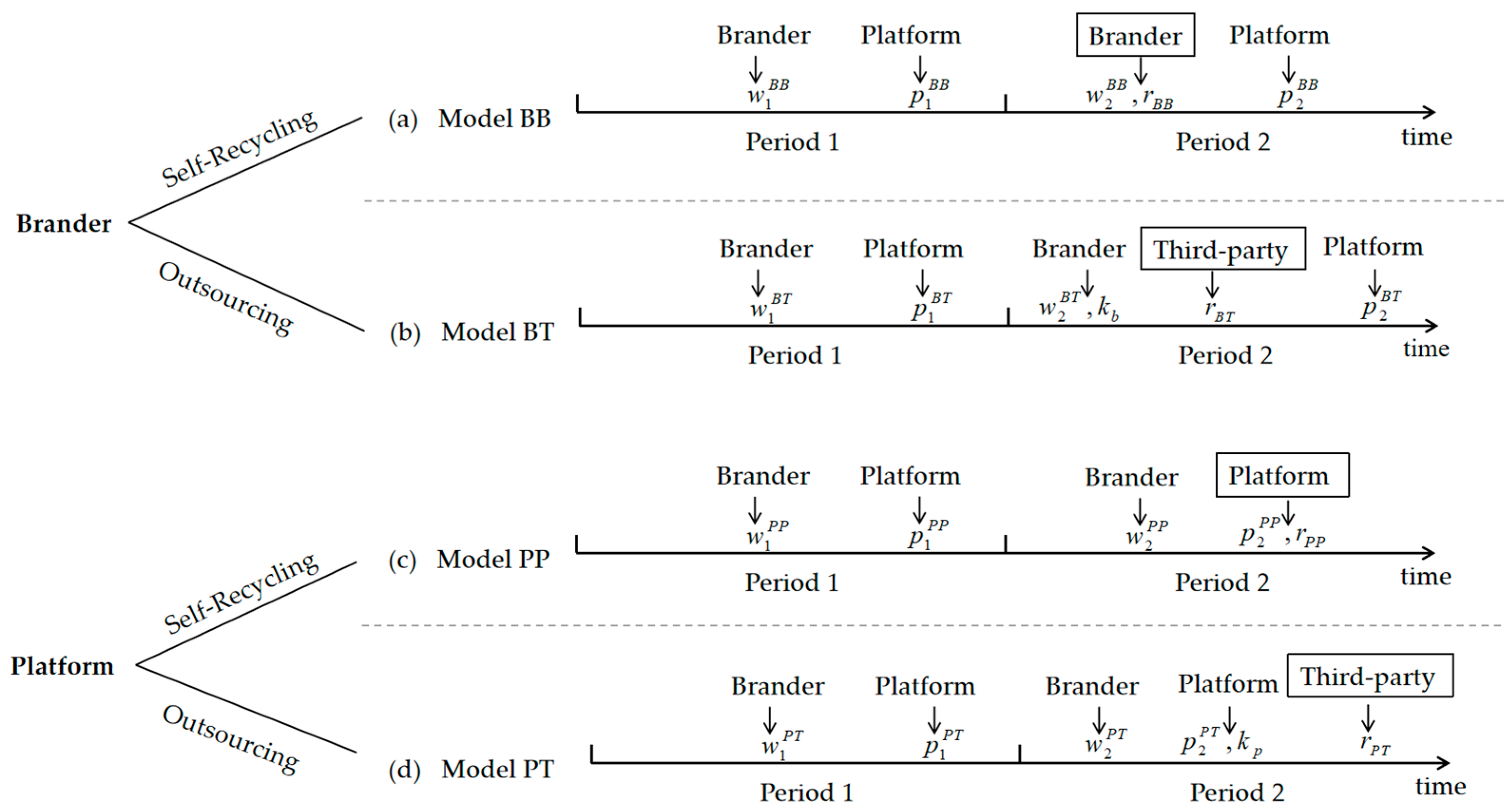
- Model BB: The brander manages the recycling process by itself, encompassing both the handling of old products and the issuance of rebates to consumers, such as IKEA’s “Buy Back & Resell” program. In period 2, the decision variables for the brander are the wholesale price and the rebate amount , while the platform is solely responsible for setting the selling price . The corresponding decision-making sequence is depicted in Figure 1a.
- Model BT: The brander outsources the recycling to a 3P, similarly to Apple’s trade-in service in cooperation with Aihuishou, Alchemy, and so on. In this model, it is assumed that the brander pays a unit commission per item. The decision variables in period 2 are extended to include the wholesale price and the outsourcing commission . Subsequently, the 3P is responsible for recycling and processing the old products and providing the rebate to consumers. Meanwhile, the platform remains solely responsible for determining the selling price . This decision sequence is illustrated in Figure 1b.
- Model PP: The platform takes full responsibility for the recycling of old products and directly offers rebates to consumers, just as Amazon receives old products and resells them after processing them itself. As a result, in period 2, the brander only determines the wholesale price , whereas the platform simultaneously determines both the selling price and the rebate amount . The decision-making sequence is illustrated in Figure 1c.
- Model PT: Following the trade-in service of Jingdong, where the recycling process is outsourced to Aihuishou, the platform outsources the recycling of the old product to a 3P and pays a unit commission for each returned item. In period 2, the brander only sets the wholesale price , whereas the platform’s decision variables include both the selling price and unit commission . The 3P assumes responsibility for processing old products and providing rebates to consumers. The decision sequence is illustrated in Figure 1d.
3.2. Customer Demand
4. Model Analysis
4.1. Brander-Led Models
4.1.1. Model BB
4.1.2. Model BT
4.2. Platform-Led
4.2.1. Model PP
4.2.2. Model PT
4.3. Equilibrium Analysis
- (1)
- , , , , ,
- (2)
- , , , , , ()
- (1)
- If , then . Otherwise,if , then .
- (2)
- . Thus,the optimal platform profit increases as the market potential increases.
- (1)
- If , then . Otherwise,if , then .
- (2)
- . Thus,the optimal platform profit increases as the market potential increases.
- (1)
- , , , , ,
- (2)
- , , , , , ()
- (1)
- . Thus,the optimal brander profit increases as the market potential increases.
- (2)
- If , then . If , then .
- (1)
- . Thus,the brander’s optimal profit increases as the market potential increases.
- (2)
- If , then ; If , then .
5. Strategy Analysis
5.1. Brander-Led vs. Platform-Led
- (i)
- In period 1:
- (1)
- If , then and .
- (2)
- The selling price is higher in period 1 under brander-led recycling (i.e., , ), whereas the consumer demand in period 1 is greater under platform-led recycling (i.e., , ).
- (ii)
- In period 2:
- (1)
- If , then and .
- (2)
- The selling price is higher in period 2 under platform-led recycling (i.e., , ).
- (3)
- In self-recycling,the rebate provided is greater under the brander-led model(i.e.,), while in the outsourcing model,it is greater under the platform-led model(i.e.,).
- (1)
- If , when , . Otherwise,if , when , .
- (2)
- If , when , . Otherwise,if , when , .
- (1)
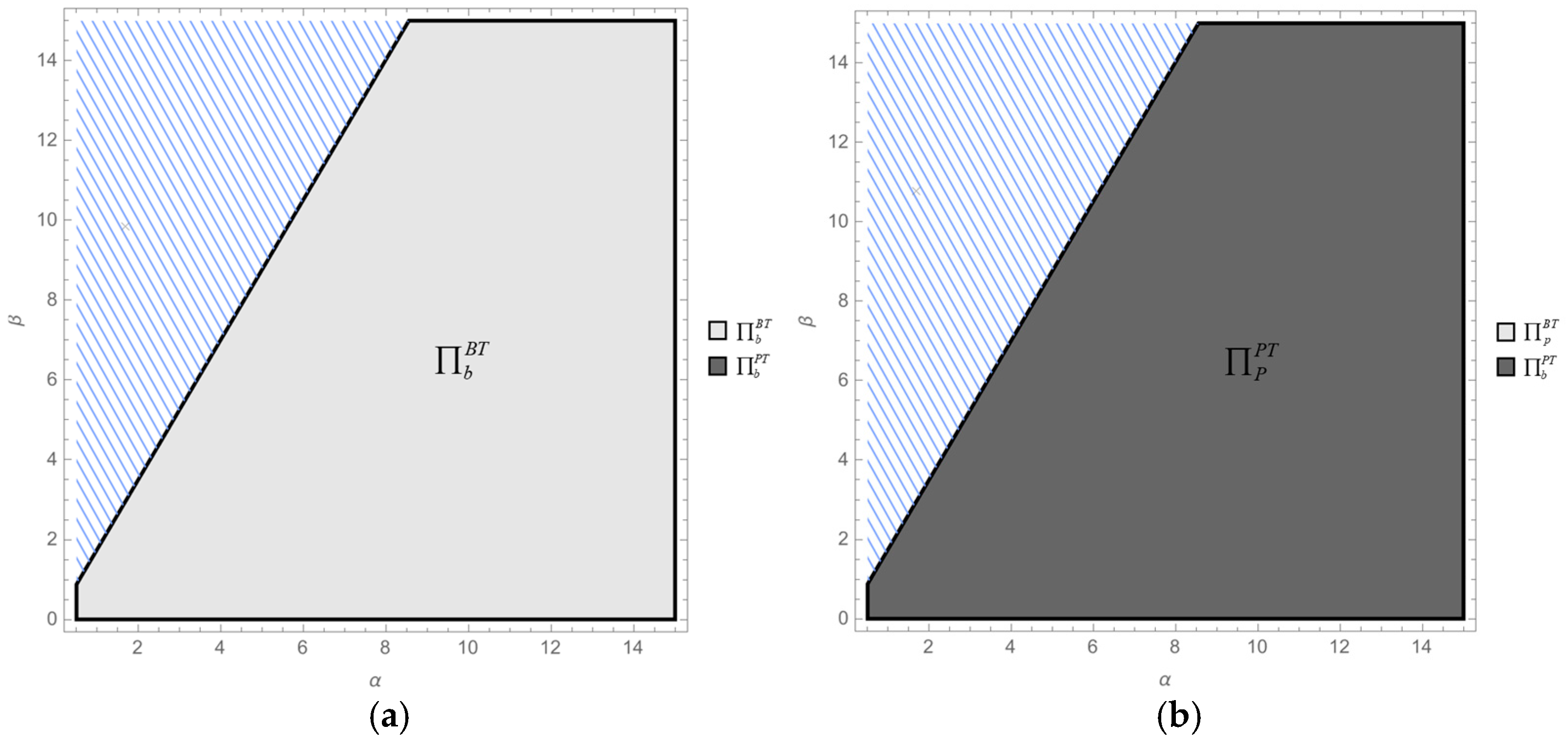
- , and the Brander prefers Model BT to PT.
- (2)
- , and the Platform prefers Model PT to BT.
- (1)
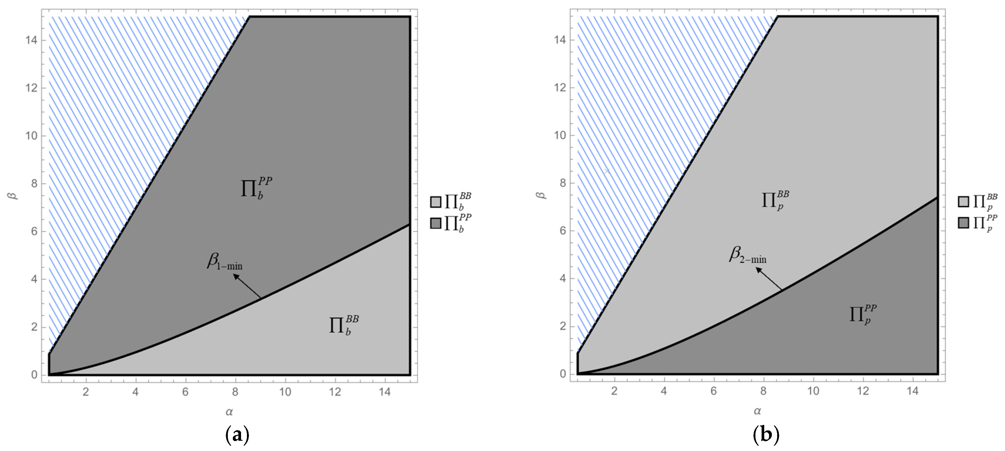
- If , the supply chain prefers Model PP over BB.
- (2)
- If , then and the supply chain prefers Model PT over BT.
5.2. Self-Recycling vs. Outsourcing
- (i)
- In period 1:
- (1)
- If , then and .
- (2)
- The selling price in period 1 is higher in outsourcing recycling (i.e.,,), whereas the consumer demand in period 1 is greater in self-recycling (i.e.,, ).
- (ii)
- In period 2:
- (1)
- If , then and .
- (2)
- If , then and .
- (3)
- If , then and .
- (1)
- When , if or , then ; if , then ; otherwise,when , then .
- (2)
- If , then ; otherwise,if , then .
- (1)
- If , then ; otherwise,if , then .
- (2)
- When , if or , then ; otherwise,if , then .
- (1)
- , and the supply chain prefers Model BB to BT.
- (2)
- , and the supply chain prefers Model PP to PT.
5.3. Optimal Model Selection
- (1)
- If , then .
- (2)
- If , then .
6. Extension
6.1. Reusing Salvage Value
- (1)
- If and , or , then .
- (2)
- If , then .
- (1)
- ; .
- (2)
- ; .
- (3)
- If , then , while .
- (4)
- If and , then , while .
6.2. Revenue-Sharing Mechanism
7. Conclusions and Suggestions
7.1. Conclusions
- (1)
- The consumer price sensitivity is an important factor influencing the choice of the dominant party. Conflicts and “free-riding” behaviors arise between the brander and the platform regarding the recycling model selection in markets characterized by different levels of price sensitivity. In low price sensitivity markets, both branders and platforms tend to choose self-recycling to obtain closed-loop benefits, while in high price sensitivity markets, both parties prefer that the other party take the lead in recycling.
- (2)
- The consumer price sensitivity and market potential jointly affect the dominant party’s choice of the recycling model. When the consumer price sensitivity is extremely high or extremely low, the dominant party should adopt self-recycling. At moderate sensitivity levels, outsourcing becomes the preferred option. However, when the market potential is high, adopting self-recycling can achieve a relative win–win outcome for both parties in the supply chain.
- (3)
- During the trade-in process, both the brander and platform can lead in recycling. The trade-in leadership significantly influences the brander’s pricing system. The platform consistently maintains a penetration pricing strategy, lowering product prices in period 1 to forgo part of its short-term profits and enhance future gains during the trade-in phase. When the brander leads recycling, it should cooperate with the platform by lowering the wholesale price in period 1, especially given the accelerating nature of product iteration cycles. Conversely, when the platform leads recycling, the brander can appropriately raise the wholesale price to optimize its own profitability.
- (4)
- When the brander leads recycling, the acquisition of the salvage does not affect the profits of supply chain members. While self-recycling by the brander could bring a win–win outcome in high price sensitivity markets, in platform-led models, branders can only profit from the acquisition of the salvage in low price sensitivity markets.
7.2. Management Insights
- (1)
- For both the brander and the e-commerce platform, it is essential to consider the influence of the consumer price sensitivity when formulating trade-in strategies. For branders involved in luxury goods, high-end products, or professional equipment, customers typically place a greater emphasis on the quality or brand value rather than the product’s price itself, therefore exhibiting low price sensitivity. Under these circumstances, both the brander and the platform can achieve higher closed-loop profits by adopting a self-recycling model for trade-in operations. In contrast, for branders involved in the daily necessities sector, consumers are more inclined to compare prices across multiple sources and are highly sensitive to price changes. In such cases, the brander and the platform must carefully deliberate the allocation of the leadership in recycling to avoid conflicts and may maximize their overall profits through compensation mechanisms or collaborative approaches.
- (2)
- Under an economic downturn the dominant party responsible for recycling should comprehensively consider the consumer price sensitivity and market size when selecting the recycling mode. In industries involving daily necessities, where consumers exhibit a high sensitivity to price changes, the dominant party should adopt a self-recycling model. Conversely, for branders with high customer loyalty, where the consumer price sensitivity is relatively low, either the brander or the collaborating platform should outsource recycling activities to save costs. These recommendations are particularly relevant for branders and platforms with limited market potential, for which the achievable economies of scale are constrained. When selecting a trade-in model, they should carefully evaluate the trade-off between the benefits and costs of recycling in light of their market potential. For large e-commerce platforms and well-known branders, a broad customer base, strong brand recognition, and a high product replacement frequency collectively contribute to substantial market potential. These branders and platforms are better positioned to establish self-recycling systems. Therefore, adopting a self-recycling model is recommended in such contexts.
- (3)
- Pricing strategies should be reasonably adjusted based on the market demand and product iteration under different recycling leadership models to balance trade-in costs and profits, thus optimizing the overall supply chain efficiency. When the brander leads recycling, both the brander and platform should appropriately lower their prices in period 1 (especially under a short product iteration cycle), in order to attract more consumers to participate in the trade-in program. Simultaneously, the brander should actively consider reusing the salvage derived from traded-in products as part of reproduction processes in order to achieve resource reuse, enhance the supply chain’s sustainability, and attract more customers to replace their high energy-consuming products. When the platform leads recycling the brander should consider moderately increasing the wholesale price under a short product iteration cycle, while platforms should maintain a penetration pricing strategy in period 1. Furthermore, when reselling high-end products, luxury brands, or professional equipment, the brander should acquire the salvage of old products from the platform for reuse in production, thus enhancing the brand’s reputation.
7.3. Limitations and Future Studies
Author Contributions
Funding
Data Availability Statement
Conflicts of Interest
Appendix A

- (1)
- In Model BB: , , , , .In Model BT: , , , , , .
- (2)
- In Model BB: ,, , , .In Model BT: , , , , , . □
- (1)
- .When , ; i.e.,.When , .
- (2)
- . □
- (1)
- .When ; i.e., .When , .
- (2)
- . □
- (1)
- In Model PP: , , , , .In Model PT: , , ,, , .
- (2)
- In Model PP: ,, , , .In Model PT: , , ,, , . □
- (1)
- .
- (2)
- .When , .When , , in which . □
- (1)
- .
- (2)
- .When , .When , , in which . □
- (i)
- In period 1:
- (1)
- Compare the wholesale price in period 1 under the self-recycling models (Models BB and PP): . When , . When , . Then, compare the wholesale price in period 1 under the outsourcing models (Models BT and PT): . When , . When , , in which . As , if , then and .
- (2)
- and . Hence, and hold universally. In addition, and . Hence, and hold universally.
- (ii)
- In period 2:
- (1)
- Compare the wholesale price in period 2 under the self-recycling models (Models BB and PP): . When (i.e., ), then . When , . Then, compare the wholesale price in period 2 under the outsourcing models (Models BT and PT): . When (i.e., ), . When , . Therefore, if , then and .
- (2)
- ; i.e., holds universally. In addition, ; i.e., holds universally.
- (3)
- ; i.e., holds universally. In addition, ; i.e., holds universally. □
- (1)
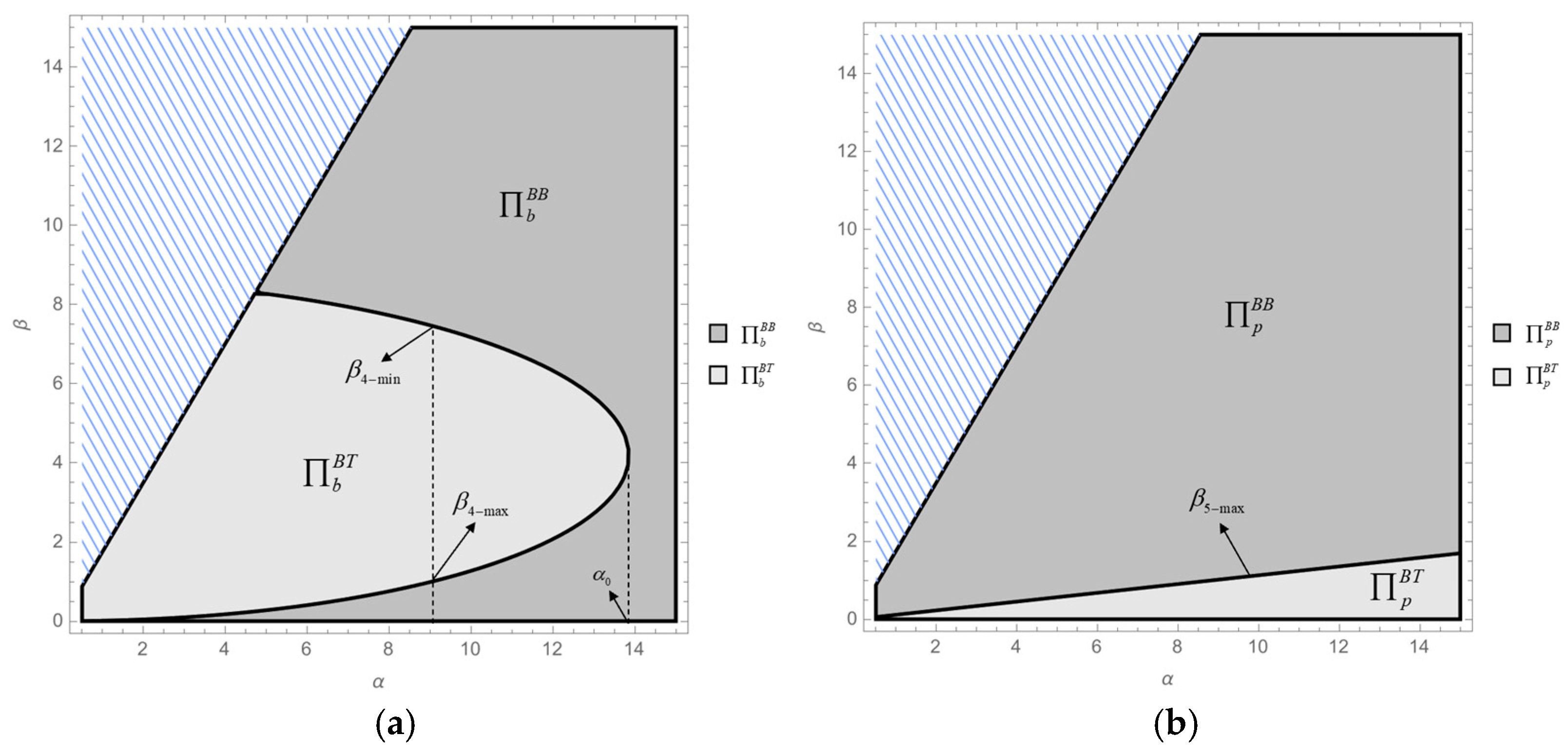
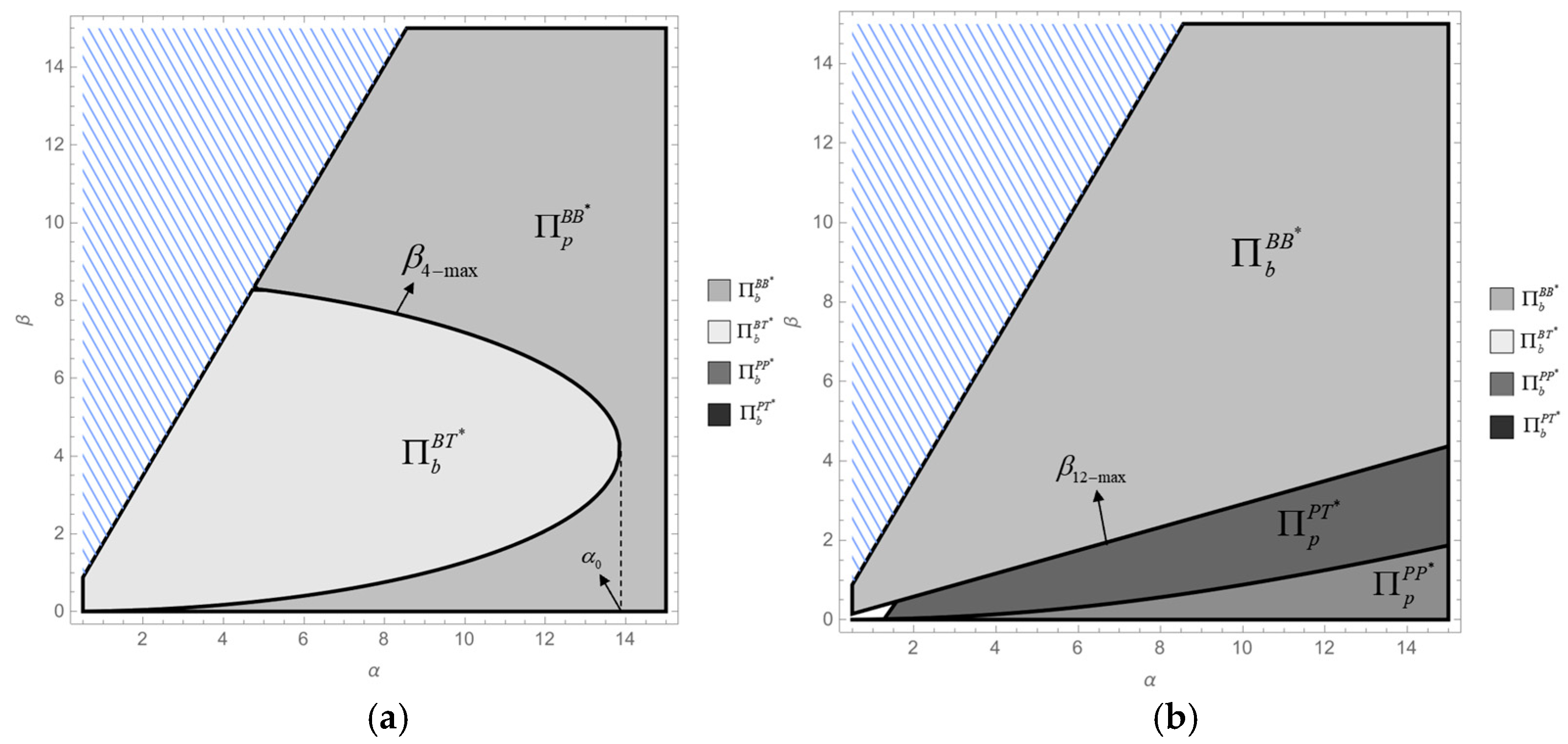
- Compare the brander’s profit between Models BB and PP:,. Therefore, . Assuming that , then is a continuous and concave function. Solving , two distinct zeros are obtained:,.Thus, when , under the given condition , the function has exactly one zero . Hence, if , then ; i.e., . Otherwise, if , then . This result is consistent with Figure 1a.
- (2)
- Compare the platform’s profit between Models BB and PP:, .Hence, . Assuming that , then is a continuous and convex function. Solving , two distinct zeros are obtained:,.Thus, when , under the given condition , the function has exactly one zero, . Hence, if , then ; i.e., . Otherwise, if , then .As , then if , the conclusions of Corollary 3(1) and Corollary 3(2) both hold with . This result is consistent with Figure 1b. □
- (1)
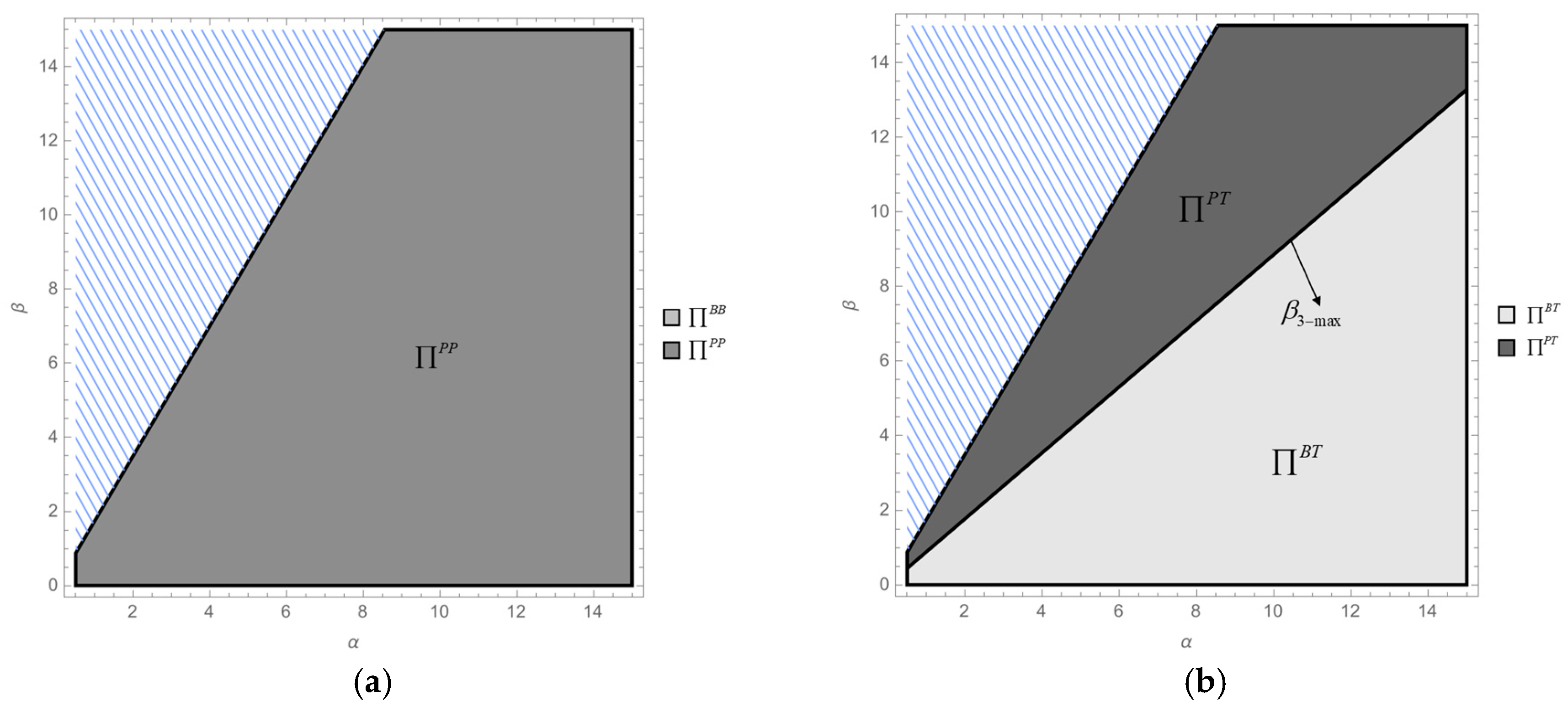
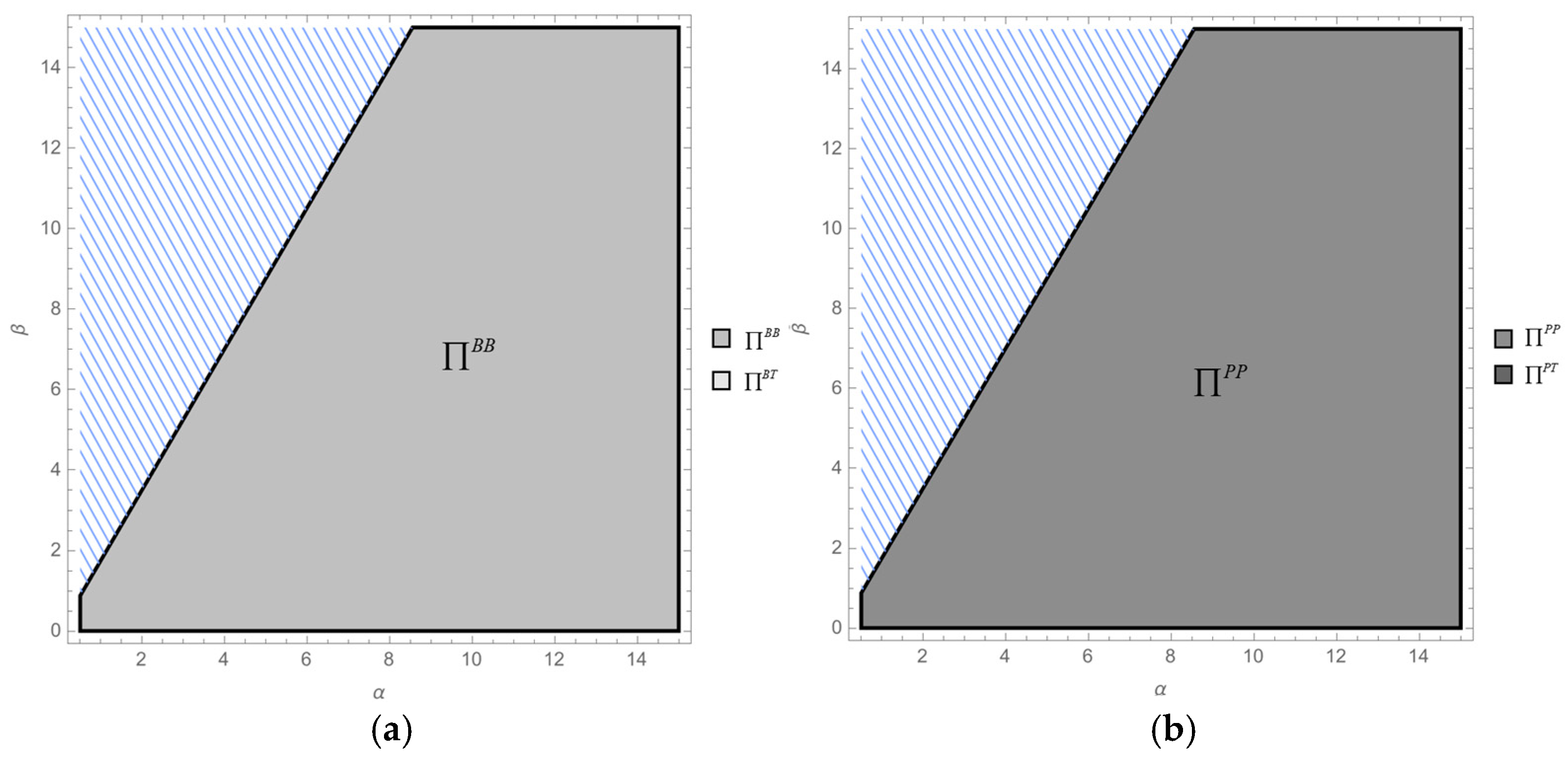
- Compare the whole supply chain profit between Models BB and PP:,.Thus, holds universally; i.e., . This result is consistent with Figure 4a.
- (2)
- Compare the whole supply chain profit between Models BT and PT:,.Thus, . Assuming that , then is a continuous and convex function. Solving , two distinct zeros are obtained:,.Thus, under the given condition , the function has exactly one zero, . Hence, if , then ; i.e., . Otherwise, if , then . This result is consistent with Figure 4b. □
- (1)
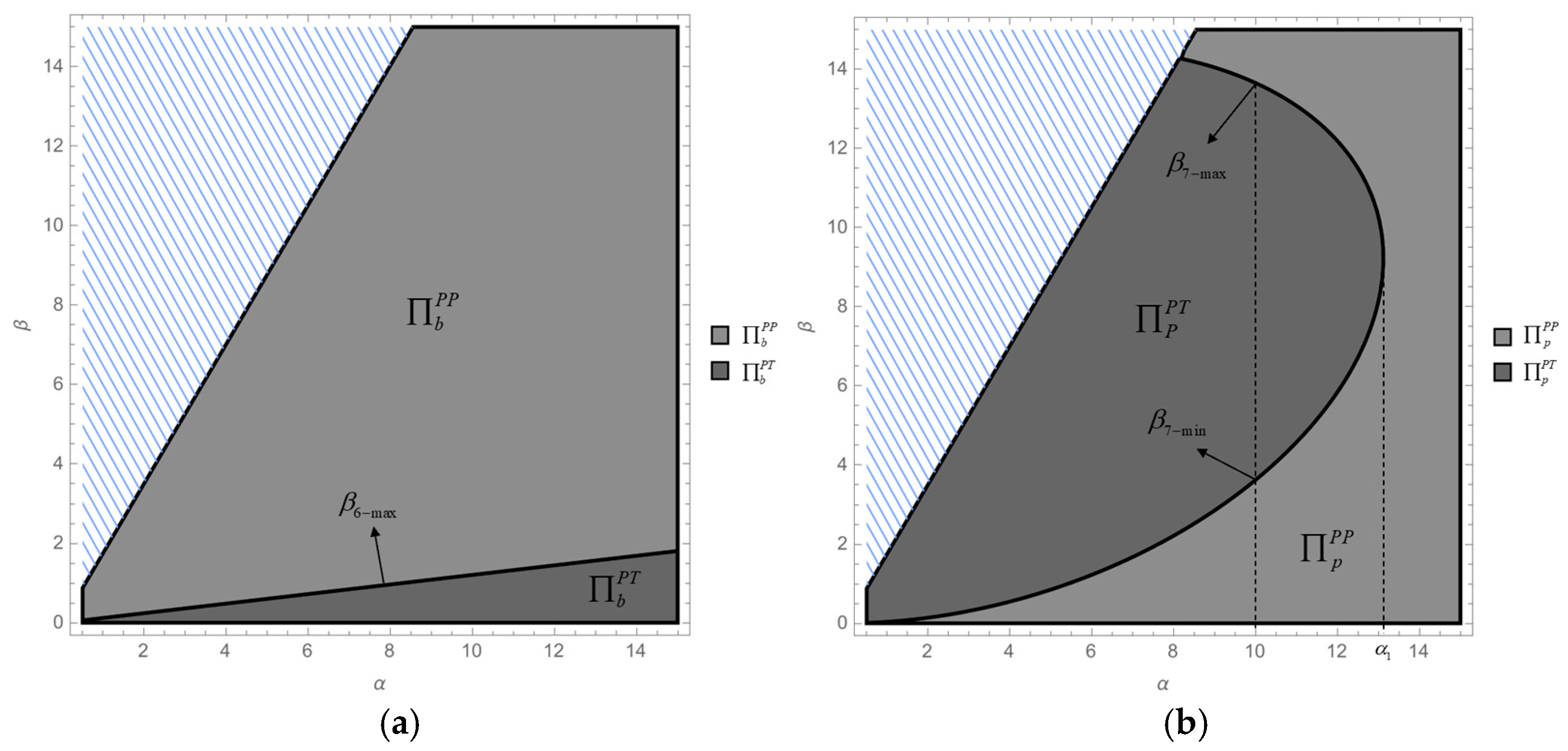
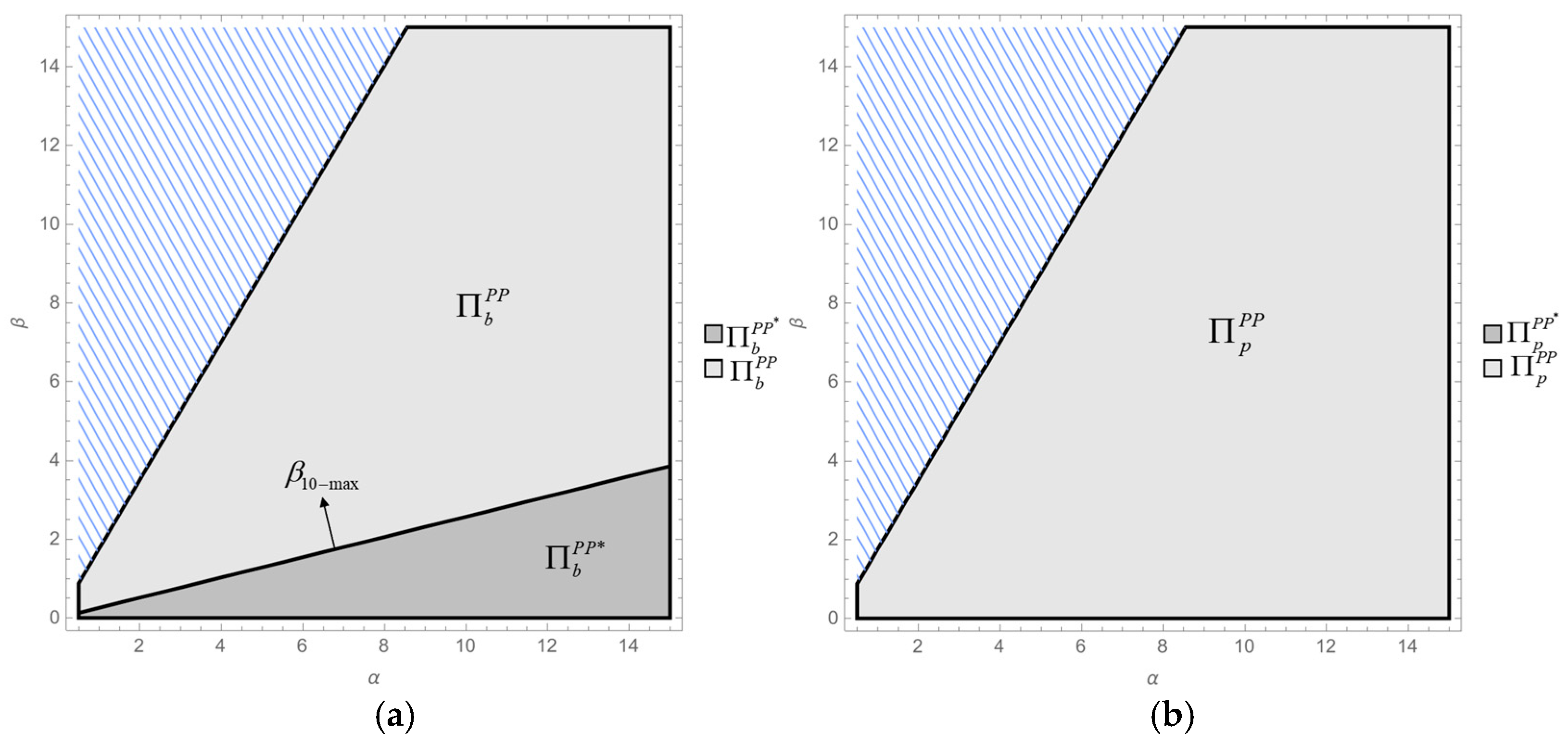
- . The remaining calculation process is similar to that of Corollary 2, where,.In particular, and .Thus, when , if or , then ; i.e., . If , then . Otherwise, when , . This result is consistent with Figure 5a.
- (2)
- . Assuming that , then is a continuous and concave function. Solving , two distinct zeros are obtained:, , in which and . Hence, under the given condition , the function has exactly one zero, .Thus, if , then ; i.e., . Otherwise, if , then . This result is consistent with Figure 5b. □
- (1)
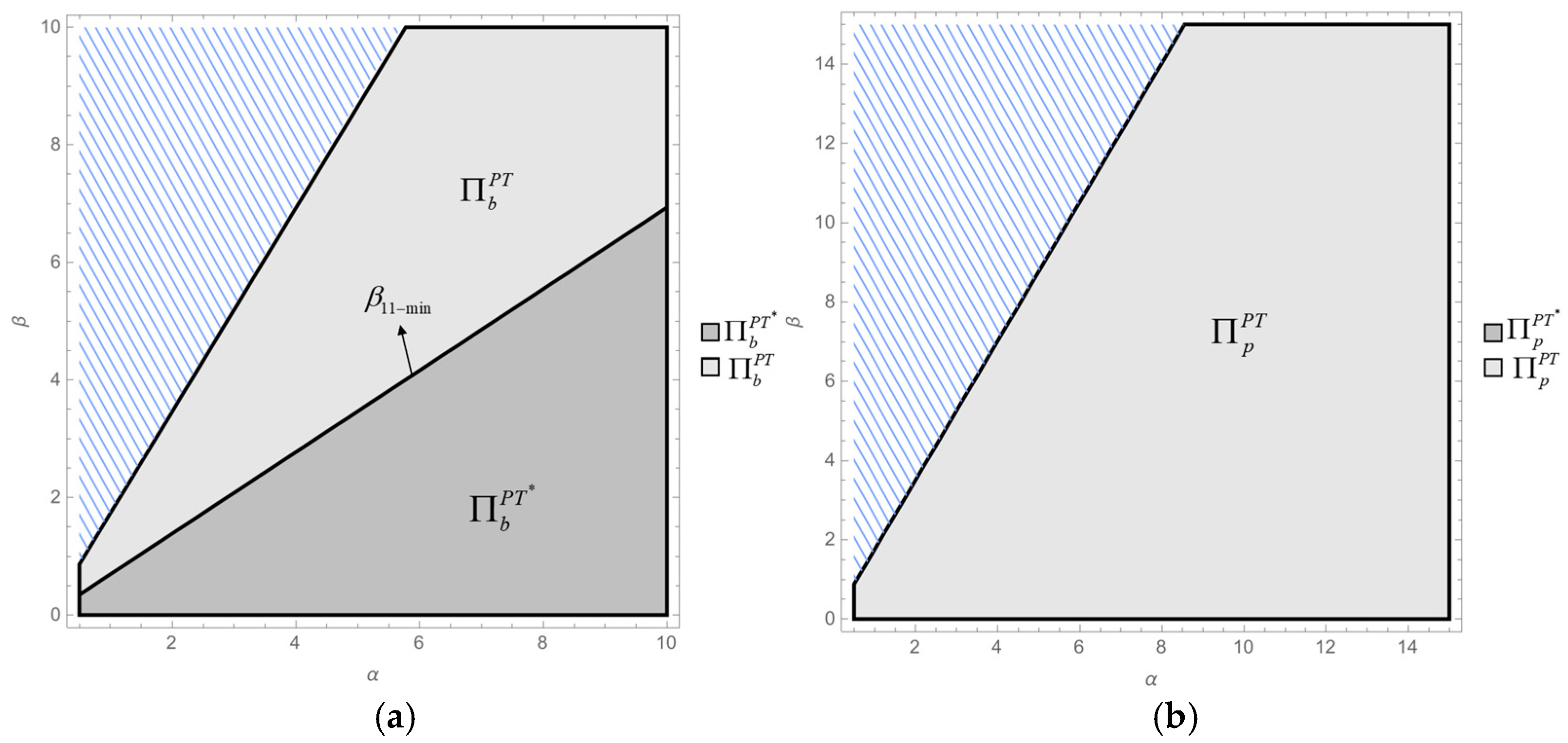
- . Assuming that , then is a continuous and concave function. Solving , two distinct zeros are obtained: , , in which and . Hence, under the given condition , the function has exactly one zero, .Thus, if , then ; i.e., . Otherwise, if , then . This result is consistent with Figure 6a.
- (2)
- , assuming that , then is a continuous and concave function. Then, , and there exists an extremum point such that the original function is monotonically decreasing when (i.e., ) and monotonically increasing when . As a result, the original function has two zeros when . Solving this yields the range of as , where . Hence, two distinct zeros are obtained:,, in which and .When , the zeros exist. Therefore, if or , then . If , then . When , . This result is consistent with Figure 6b. □
- (1)
- Compare the whole supply chain profits under brander-led models (Models BB and BT):As and, . As a result, holds universally. This result is consistent with Figure 7a.
- (2)
- Compare the whole supply chain profits under platform-led models (Models PP and PT):As and , . As a result, holds universally. This result is consistent with Figure 7b. □
- (1)
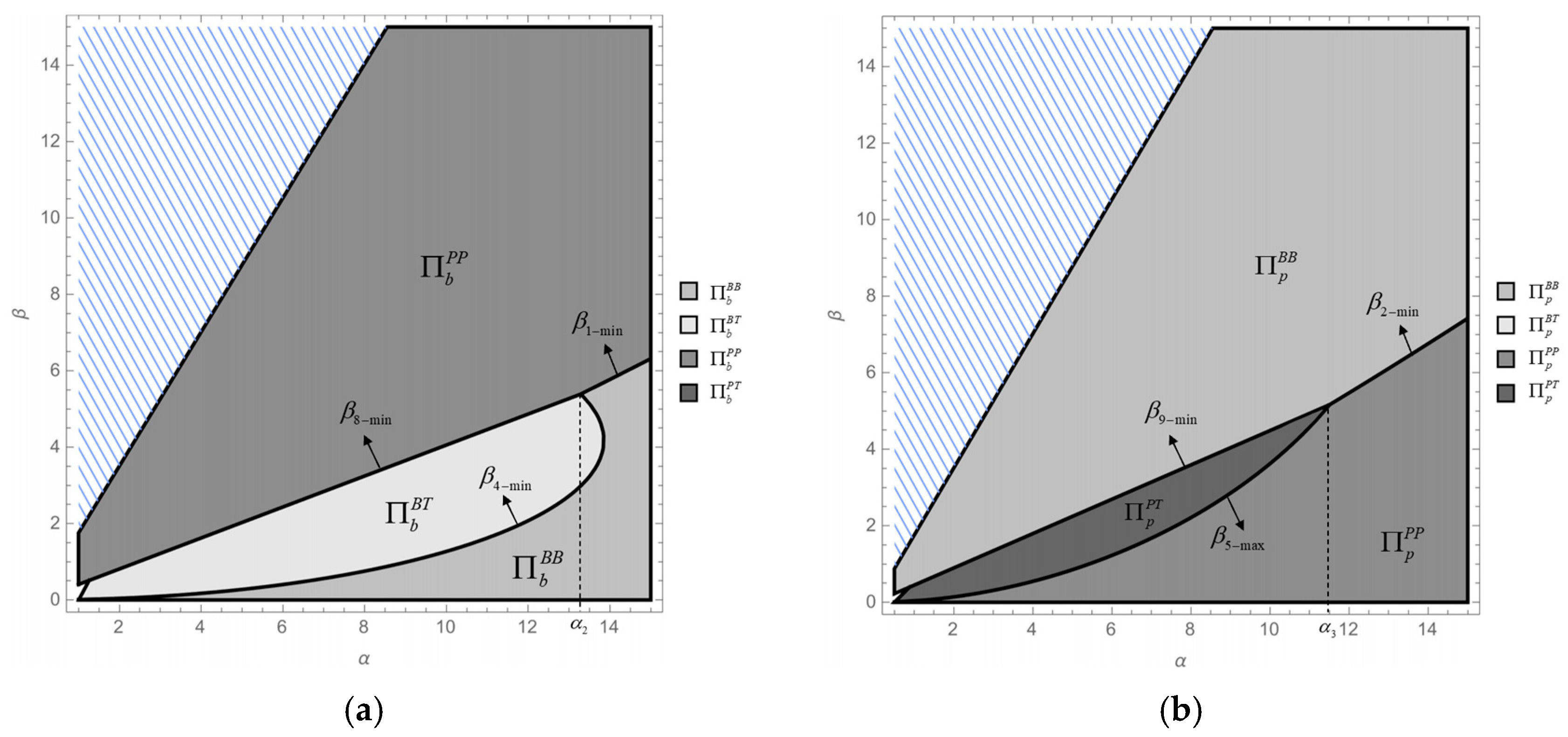
- It is shown in Corollaries 3, 4, and 8 that if , then . Furthermore, if , then , in which . Moreover, holds universally.When :If or , then ; i.e., . If , then . If , then , in which and .As and , . Assuming that , then is a continuous and convex function. Solving , two distinct zeros are obtained:, , in which and . Hence, under the given condition , the function has exactly one zero, . Therefore, if , then ; i.e., . If , then .When .Hence, , where .exists when , and . Moreover, when ,Therefore, and exist when . As holds universally, when and , .When :and exist when . As holds universally, when and , .In summary, when , . This result is consistent with Figure 8a.
- (2)
- It is shown in Corollaries 3, 4, and 8 that if , then . Otherwise, if , then , in which . Secondly, holds universally. Thirdly, if , then . Otherwise, if , then , in which .As and , . Assuming that , then is a continuous and convex function. Solving , two distinct zeros are obtained:, , in which and . Hence, under the given condition , the function has exactly one zero, . Therefore, if , then ; i.e., .As , if , then , in which . Therefore, and exist when . Given that holds universally, there exists .Otherwise, if , then ; i.e., . Hence, and exist when . Given that holds universally, there exists .In summary, if , then . This result is consistent with Figure 8b. □
- Model BB*: As the brander independently recycles and processes the salvage in this model, there is no transfer pricing of the salvage. Thus, the profits stay the same as in the original Model BB.
- Model BT*: The cost paid by the brander to acquire the salvage replaces the commission in the original model, while the other components of profit remain unchanged. Therefore, the game player’s maximum profit is as follows:
- Model PP*: Based on the original assumptions, the brander pays the platform a transfer price for the salvage and receives the processed salvage in return. Therefore, the game player’s maximum profit is as follows:
- Model PT*: Similarly to Model PP*, the game player’s maximum profit is as follows:
| Equilibrium | Model BB* | Model BT* | Model PP* | Model PT* |
|---|---|---|---|---|
| - | - | - | ||
| - | ||||
| - | - |
- (1)
- Comparing the brander’s profit in different models,,,.As a result, the brander’s profit can meet the highest level only in brander-led models (i.e., Models BB* and BT*). As and the remaining calculation follows the same procedure as in Corollary 11. This result is consistent with Figure 9a.
- (2)
- Comparing the platform’s profit in different models, assuming that , then is a continuous concave function. Solving , two distinct zeros are obtained:, .As , under the given condition , the function has exactly one zero, . Thus, if , then ., assuming that , then is a continuous and concave function. Solving , two distinct zeros are obtained:,, in which and . Hence, under the given condition , the function has exactly one zero, . Therefore, if , then .As holds universally, if , then and .Combined with Corollary 8, we can state that if , then , in which . As holds universally, if , then , , and exist at the same time; i.e., . This result is consistent with Figure 9b. □
- (1)
- From the Table A2, we have that and .
- (2)
- From the Table A1, we have that and .
- (3)
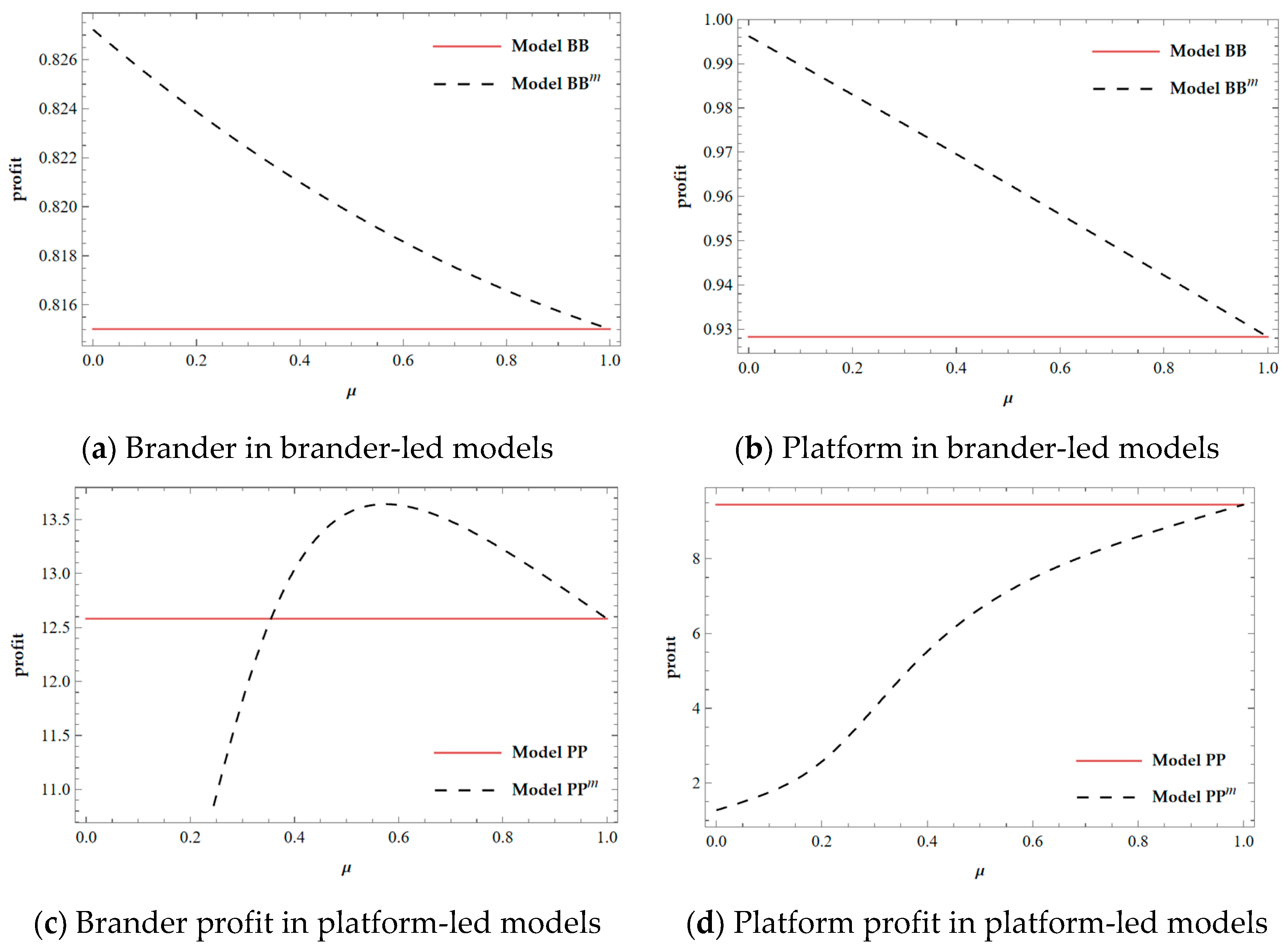
- .Assuming that , then is a continuous and convex function. Solving two distinct zeros are obtained:,Hence, under the given condition , the function has exactly one zero, . Therefore, if , then ; i.e., . Otherwise, if , then .When , holds universally; i.e., . This result is consistent with Figure 10.
- (4)
- . Assuming that , then is a continuous and concave function. Solving , two distinct zeros are obtained: , . When there is only one zero, , in which . Meanwhile, if , then ; i.e., .When , holds universally; i.e., . This result is consistent with Figure 11. □
References
- Dou, G.; Ma, L.; Wei, K.; Zhang, Q. (Eds.) Does Implementing Trade-In and Green Technology Together Benefit the Environment? In Operations Management for Environmental Sustainability: Operational Measures, Regulations and Carbon Constrained Decisions; Springer International Publishing: Cham, Switzerland, 2023; pp. 85–121. ISBN 978-3-031-37600-9. [Google Scholar]
- Bai, J.; Hu, S.; Gui, L.; So, K.C.; Ma, Z. Optimal Subsidy Schemes and Budget Allocations for Government-subsidized Trade-in Programs. Prod. Oper. Manag. 2021, 30, 2689–2706. [Google Scholar] [CrossRef]
- Zheng, B.; Cai, Y.; Li, S. Trade-in and Resale in a Platform Supply Chain: Manufacturer’s Choice of Selling Strategies. Transp. Res. Part E Logist. Transp. Rev. 2025, 193, 103836. [Google Scholar] [CrossRef]
- China News Service. Last Year, the Trade-in of Old Products for New Ones Boosted the Consumption of Home Appliances by 270 Billion Yuan. Available online: https://www.china-news-online.com/lang/English/4235729.html (accessed on 8 May 2025).
- Wang, R.; Du, Y.; Wei, Y. Does the Bike-Sharing Platform Share Its Own Private Information or Not in a Reverse Supply Chain? Sustainability 2024, 16, 9194. [Google Scholar] [CrossRef]
- Ma, D.-Q.; Wang, X.-Q.; Wang, X.; Hu, J.-S. Achieving Triple Benefits in a Platform-Based Closed-Loop Supply Chain: The Optimal Combination between Recycling Channel and Blockchain. Sustainability 2023, 15, 3921. [Google Scholar] [CrossRef]
- Mazzucchelli, A.; Chierici, R.; Del Giudice, M.; Bua, I. Do Circular Economy Practices Affect Corporate Performance? Evidence from Italian Large-Sized Manufacturing Firms. Corp. Soc. Responsib. Environ. Manag. 2022, 29, 2016–2029. [Google Scholar] [CrossRef]
- Yang, V. JD.com Partners with Leading Home Brands to Launch Green Trade-in Alliance. Available online: https://jdcorporateblog.com/jd-com-partners-with-leading-home-brands-to-launch-green-trade-in-alliance/ (accessed on 12 February 2025).
- Hu, S.; Ma, Z.-J.; Sheu, J.-B. Optimal Prices and Trade-in Rebates for Successive-Generation Products with Strategic Consumers and Limited Trade-in Duration. Transp. Res. Part E Logist. Transp. Rev. 2019, 124, 92–107. [Google Scholar] [CrossRef]
- Yi, Y.; Chen, J.; Feng, J. Optimizing Prices in Trade-in Strategies for Vehicle Manufacturers. Comput. Ind. Eng. 2021, 157, 107338. [Google Scholar] [CrossRef]
- Xiao, Y. Choosing the Right Exchange-Old-for-New Programs for Durable Goods with a Rollover. Eur. J. Oper. Res. 2017, 259, 512–526. [Google Scholar] [CrossRef]
- Zhao, W.; Xia, Y.; Zhang, L.; Fan, X. Trade-in Program Options in a Retailer-led Supply Chain. In International Transactions in Operational Research; Wiley Online Library: Montreal, QC, Canada, 2024; p. itor.13574. [Google Scholar] [CrossRef]
- Wang, W.; Feng, L.; Chen, X.; Yang, L.; Choi, T.-M. Impacts of Selling Models: Who Should Offer Trade-in Programs in e-Commerce Supply Chains? Transp. Res. Part E Logist. Transp. Rev. 2024, 186, 103524. [Google Scholar] [CrossRef]
- Yu, Z.; Wang, Y.; Shen, L.; Ji, X. Decision Making by Trade-In Programs in the E-Commerce Supply Chain, Considering Cash Rebate Strategies and Platform Services. Mathematics 2024, 12, 3792. [Google Scholar] [CrossRef]
- Bonina, C.; Koskinen, K.; Eaton, B.; Gawer, A. Digital Platforms for Development: Foundations and Research Agenda. Inf. Syst. J. 2021, 31, 869–902. [Google Scholar] [CrossRef]
- Zhang, Z.; Xu, H.; Chen, K.; Zhao, Y.; Liu, Z. Channel Mode Selection for an E-Platform Supply Chain in the Presence of a Secondary Marketplace. Eur. J. Oper. Res. 2023, 305, 1215–1235. [Google Scholar] [CrossRef]
- Guo, L.; Zhang, Q.; Wu, J.; Santibanez Gonzalez, E.D.R. An Evolutionary Game Model of Manufacturers and Consumers’ Behavior Strategies for Green Technology and Government Subsidy in Supply Chain Platform. Comput. Ind. Eng. 2024, 189, 109918. [Google Scholar] [CrossRef]
- Pan, W.; Lin, M. A Two-Stage Closed-Loop Supply Chain Pricing Decision: Cross-Channel Recycling and Channel Preference. Axioms 2021, 10, 120. [Google Scholar] [CrossRef]
- Li, D.; Cruz, J.M.; Ke, K. Closed-Loop Supply Chain Network Model with Recycling, Re-Manufacturing, Refurbishing, and Corporate Social Responsibility. Ann. Oper. Res. 2025, 345, 247–275. [Google Scholar] [CrossRef]
- Yang, Q.; Sun, L. Eco-Design in Manufacturing or Remanufacturing? The Sustainable Options in a Closed-Loop Supply Chain with Outsourcing. Sustainability 2024, 16, 1633. [Google Scholar] [CrossRef]
- Li, Y.; Wang, K.; Xu, F.; Fan, C. Management of Trade-in Modes by Recycling Platforms Based on Consumer Heterogeneity. Transp. Res. Part E Logist. Transp. Rev. 2022, 162, 102721. [Google Scholar] [CrossRef]
- Cao, K.; Gong, Y.; Xu, Y.; Wang, J. Optimal Trade-in Delegation Strategy Considering Third-Party Recycler Intrusion and Used Products with Different Durability. Oper. Res. 2025, 25, 1. [Google Scholar] [CrossRef]
- Zheng, B.; Chu, J.; Jin, L. Recycling Channel Selection and Coordination in Dual Sales Channel Closed-Loop Supply Chains. Appl. Math. Modell. 2021, 95, 484–502. [Google Scholar] [CrossRef]
- Li, H.; Yi, Y. Optimal Trade-in Rebate Payment Strategies for B2C Platforms under Different Recycling Models. J. Ind. Manag. Optim. 2024, 20, 1395–1434. [Google Scholar] [CrossRef]
- Ferrer, G.; Swaminathan, J.M. Managing New and Remanufactured Products. Manag. Sci. 2006, 52, 15–26. [Google Scholar] [CrossRef]
- Yin, R.; Tang, C.S. Optimal Temporal Customer Purchasing Decisions under Trade-In Programs with up-Front Fees. Decis. Sci. 2014, 45, 373–400. [Google Scholar] [CrossRef]
- Quan, Y.; Hong, J.; Song, J.; Leng, M. Game-Theoretic Analysis of Trade-in Services in Closed-Loop Supply Chains. Transp. Res. Part E Logist. Transp. Rev. 2021, 152, 102428. [Google Scholar] [CrossRef]
- Hu, S.; Tang, Y. Impact of Product Sharing and Heterogeneous Consumers on Manufacturers Offering Trade-in Programs. Omega 2024, 122, 102949. [Google Scholar] [CrossRef]
- Genc, T.S.; De Giovanni, P. Optimal Return and Rebate Mechanism in a Closed-Loop Supply Chain Game. Eur. J. Oper. Res. 2018, 269, 661–681. [Google Scholar] [CrossRef]
- Raz, G.; Souza, G.C. Recycling as a Strategic Supply Source. Prod. Oper. Manag. 2018, 27, 902–916. [Google Scholar] [CrossRef]
- Yenipazarli, A. Managing New and Remanufactured Products to Mitigate Environmental Damage under Emissions Regulation. Eur. J. Oper. Res. 2016, 249, 117–130. [Google Scholar] [CrossRef]
- Apple. Trade In. Available online: https://www.apple.com/shop/trade-in (accessed on 8 May 2025).
- Vogue. Gucci and the RealReal Announce a Game-Changing Partnership. Available online: https://www.vogue.com/article/gucci-the-realreal-partnership-secondhand-consignment (accessed on 8 May 2025).
| Research Paper | Brander-Led | Platform-Led | 2-Period | ||
|---|---|---|---|---|---|
| Self-Recycling | Outsourcing | Self-Recycling | Outsourcing | ||
| Yi et al. [10] | √ | ||||
| Bai et al. [2] | √ | ||||
| Xiao [11] | √ | ||||
| Zhao et al. [12] | √ | ||||
| Wang et al. [13] | √ | ||||
| Yu et al. [14] | √ | √ | |||
| Zheng et al. [3] | √ | ||||
| Cao et al. [22] | √ | √ | |||
| Zheng et al. [23] | √ | √ | |||
| Li &Yi [24] | √ | √ | |||
| Yin & Tang [26] | √ | √ | |||
| Quan et al. [27] | √ | √ | √ | ||
| Hu & Tang [28] | √ | √ | |||
| This paper | √ | √ | √ | √ | √ |
| Symbol | Definition | Symbol | Definition |
|---|---|---|---|
| Period , | The cost for a brander to produce new products in period | ||
| Model , (, is the extension model) | New customer demand in period | ||
| In period , brander’s wholesale price in Model | The demand from existing customers for trade-in programs | ||
| In period , the platform’s sales price under Model | Market potential | ||
| Rebate price offered in trade-in service under Model | Customer’s price sensitivity | ||
| The salvage value of old products | Brander’s profit under Model | ||
| Fixed costs for recycling old products | Platform’s profit under Model | ||
| The unit commission paid by the brander to the third-party recycler | The third-party recycler’s profit under Model | ||
| The unit commission paid by the platform to the third-party recycler | The transfer price of salvage in the extended model |
| Equilibrium | Model BB | Model BT | Model PP | Model PT |
|---|---|---|---|---|
| Wholesale in period 1: | ||||
| Sales price in period 1: | ||||
| Wholesale in period 2: | ||||
| Sales price in period 2: | ||||
| Rebate price: | ||||
| Unit commission: | - | - | ||
| Brander’s profit: | ||||
| Platform’s profit: | ||||
| The 3P’s profit: | - | - |
Disclaimer/Publisher’s Note: The statements, opinions and data contained in all publications are solely those of the individual author(s) and contributor(s) and not of MDPI and/or the editor(s). MDPI and/or the editor(s) disclaim responsibility for any injury to people or property resulting from any ideas, methods, instructions or products referred to in the content. |
© 2025 by the authors. Licensee MDPI, Basel, Switzerland. This article is an open access article distributed under the terms and conditions of the Creative Commons Attribution (CC BY) license (https://creativecommons.org/licenses/by/4.0/).
Share and Cite
Zhu, L.; Si, Y.; Han, Z. Self-Recycling or Outsourcing? Research on the Trade-In Strategy of a Platform Supply Chain. Sustainability 2025, 17, 6158. https://doi.org/10.3390/su17136158
Zhu L, Si Y, Han Z. Self-Recycling or Outsourcing? Research on the Trade-In Strategy of a Platform Supply Chain. Sustainability. 2025; 17(13):6158. https://doi.org/10.3390/su17136158
Chicago/Turabian StyleZhu, Lingrui, Yinyuan Si, and Zhihua Han. 2025. "Self-Recycling or Outsourcing? Research on the Trade-In Strategy of a Platform Supply Chain" Sustainability 17, no. 13: 6158. https://doi.org/10.3390/su17136158
APA StyleZhu, L., Si, Y., & Han, Z. (2025). Self-Recycling or Outsourcing? Research on the Trade-In Strategy of a Platform Supply Chain. Sustainability, 17(13), 6158. https://doi.org/10.3390/su17136158