Predicting Groundwater Level Dynamics and Evaluating the Impact of the South-to-North Water Diversion Project Using Stacking Ensemble Learning

Abstract

This study aims to improve the accuracy and interpretability of deep groundwater level forecasting in Cangzhou, a typical overexploitation area in the North China Plain. To address the limitations of traditional models and existing machine learning approaches, we develop a Stacking ensemble learning framework that integrates meteorological, spatial, and anthropogenic variables, including lagged groundwater levels to reflect aquifer memory. The model combines six heterogeneous base learners with a meta-model to enhance prediction robustness. Performance evaluation shows that the ensemble model consistently outperforms individual models in accuracy, generalization, and spatial adaptability. Scenario-based simulations are further conducted to assess the effects of the South-to-North Water Diversion Project. Results indicate that the diversion project significantly mitigates groundwater depletion, with the most overexploited zones showing water level recovery of up to 17 m compared to the no-diversion scenario. Feature importance analysis confirms that lagged water levels and pumping volumes are dominant predictors, aligning with groundwater system dynamics. These findings demonstrate the effectiveness of ensemble learning in modeling complex groundwater behavior and provide a practical tool for water resource regulation. The proposed framework is adaptable to other groundwater-stressed regions and supports dynamic policy design for sustainable groundwater management.

1. Introduction

1.1. Background and Significance

Groundwater is a vital strategic resource for maintaining ecological balance and supporting human development, playing an irreplaceable role in agricultural irrigation (accounting for 72% of total regional water consumption), industrial water supply, and urban living systems [1]. However, the excessive exploitation of groundwater has caused a continuous decline in water levels [2], triggering a series of ecological and environmental problems, such as land desertification, seawater intrusion, vegetation degradation [3], river drying [4], and accelerated land subsidence [5]. These issues have severely undermined the ecological equilibrium and environmental stability. Accurate prediction of groundwater level variations is essential not only for achieving sustainable water resource management but also for preventing geo-environmental disasters and safeguarding ecological security [6]. Regional differences in hydrogeological conditions add complexity to groundwater systems. In addition, variations in groundwater abstraction methods and intensities further increase the variability of groundwater level dynamics. Together, these factors present significant challenges for accurate prediction.

The Cangzhou region, in particular, is characterized by deep confined aquifers with structurally enclosed settings and limited lateral recharge. These features substantially reduce aquifer responsiveness to natural replenishment, making groundwater level forecasting more difficult and necessitating more robust and adaptable modeling approaches [7].

1.2. Limitations of Traditional Models and the Rise of Machine Learning

Traditional groundwater level prediction methods mainly rely on physically based numerical models, such as MODFLOW, GMS, and FEFLOW. These models typically describe groundwater flow using partial differential equations, which possess clear physical interpretations. However, their effectiveness is constrained by the accuracy of hydrogeological parameters, and they are computationally intensive, limiting their applicability in data-scarce environments [8]. In recent years, machine learning has gained attention as a promising alternative. It provides a data-driven modeling framework that can automatically learn complex nonlinear relationships between variables. This approach does not require predefined physical equations. This paradigm has been increasingly adopted in groundwater level forecasting research [9]. For example, Singh et al. developed an AutoML-GWL framework using Bayesian optimization, which incorporated multiple features, such as precipitation, temperature, and soil type, achieving high accuracy with an RMSE of 1.22 [10]. LaBianca et al. applied the CatBoost gradient boosting decision tree model, integrated with high-resolution urban features, to predict the minimum water table depth (MWTD), outperforming conventional physical models [11]. Azizi et al. utilized the Group Method of Data Handling (GMDH) neural network to simulate groundwater levels under climate change scenarios [12]. Despite these advancements, individual machine learning models—such as random forest—often fail to fully capture the complexity and nonlinearity of groundwater systems. This limitation is mainly due to restricted training data and the intrinsic constraints of the algorithms themselves. For instance, Lasso and Ridge regression are effective for modeling linear patterns but underperform in nonlinear environments. KNN models, on the other hand, are highly sensitive to noise and less robust to sparse or heterogeneous data distributions, resulting in unstable predictions and restricted model performance improvements [13].

Furthermore, most current machine learning models used in groundwater prediction are purely data-driven and fail to incorporate essential physical constraints, such as mass conservation. This lack of physical interpretability reduces their extrapolation capabilities, particularly under changing environmental or management scenarios. Additionally, these models often overlook the delayed response behavior of deep confined aquifers—a key aspect of groundwater system dynamics. As a result, their predictive performance and generalization ability decline when applied to complex systems like those in Cangzhou. In such regions, groundwater responses are highly inertial and are mainly governed by slow recharge processes.

1.3. Advantages of Ensemble Learning and the Stacking Approach

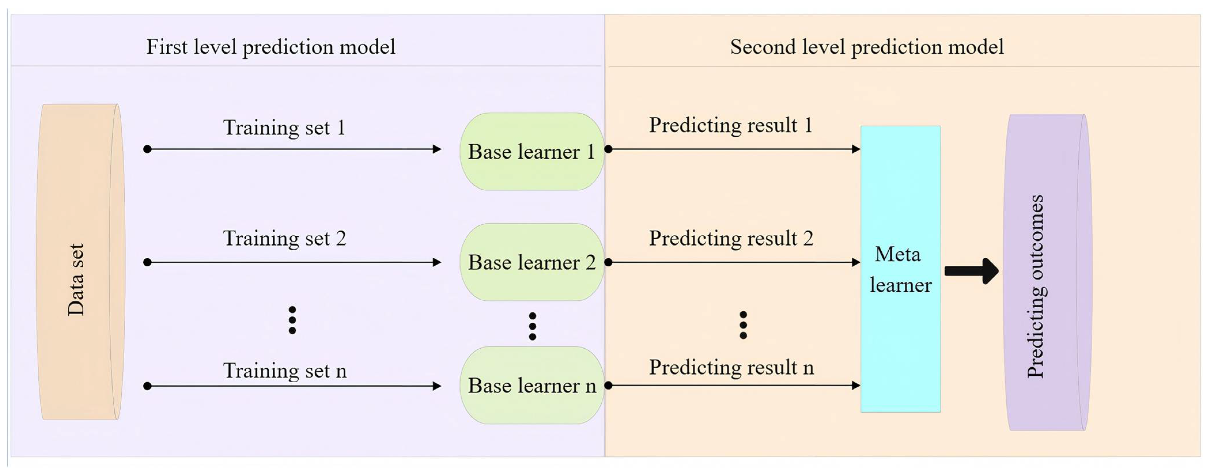
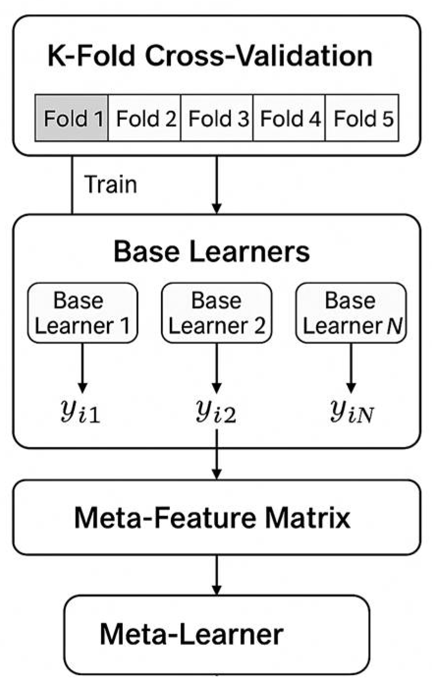
Many scholars have begun exploring ensemble learning models to overcome the limitations of individual models. Stacking is a multilayer ensemble learning method that integrates several base models, each with different predictive strengths. A meta-learner is then used to combine their outputs, producing final predictions with improved generalization capability. Unlike Bagging and Boosting, Stacking supports the integration of heterogeneous models, such as support vector machines, random forests, and neural networks, allowing it to leverage the strengths of each model in handling nonlinear relationships, feature redundancy, and high-dimensional data.

In groundwater modeling, challenges such as data noise, complex spatiotemporal scales, and nonlinear interactions are common. Stacking addresses these issues by aggregating the outputs of multiple models through secondary learning, thereby enhancing adaptability and improving prediction stability. In this study, the Stacking ensemble model is designed not only to combine multiple algorithms but also to incorporate domain knowledge by embedding lagged groundwater level terms as input features. These features reflect the delayed response of aquifers to external drivers, such as precipitation and extraction, enabling the model to capture the system’s memory and long-term behavior. This makes Stacking particularly suited for groundwater level modeling across different regions, scales, and future climate scenarios [14]. Unlike Bagging, which uses simple averaging, or Boosting, which relies on weighted summation, Stacking employs a meta-model—such as logistic regression, GBDT, or neural networks—to flexibly learn complex relationships among the predictions of base models. This approach helps overcome the limitations of using a single ensemble strategy [15]. The multi-stage ensemble model outperforms individual models in handling nonlinear, multi-scale hydrological data. For instance, Elzain deployed a stacked ensemble framework integrating multi-source data (remote sensing, meteorological, and hydrogeological data), significantly enhancing prediction robustness. Deep learning components like Transformers were incorporated to improve temporal feature extraction. In a case study in Saudi Arabia, this model achieved a 22% reduction in RMSE and an R² of 0.91, providing high-precision decision support for water resource management in water-scarce regions [16]. In a decade-long study in the Huaibei Plain, Jiang et al. applied the Stacking ensemble model for groundwater level prediction under future climate scenarios. By integrating multiple base learners, including support vector regression (SVM), random forest (RF), and multilayer perceptron (MLP), and using linear regression as the meta-learner, the model demonstrated superior performance across all monitoring wells. RMSE reductions ranged from 4.26% to 96.97%, with the lowest MAE and highest R² among all models tested [17]. In summary, ensemble learning models, especially Stacking, are more capable of capturing complex data patterns and dynamics compared to individual models, thereby improving the accuracy and stability of predictions.

1.4. Research Objective and Innovation

As a typical deep groundwater overextraction area in the North China Plain, the evolution of groundwater levels in Cangzhou is influenced by both natural processes and human activities. To address the significant spatiotemporal heterogeneity of groundwater in the region, this study proposes a Stacking ensemble model. The model integrates meteorological variables, spatial attributes, groundwater extraction intensity, and historical groundwater level time series to enhance prediction accuracy.

Through multi-model integration, the framework explores the spatiotemporal interactions between groundwater levels and multi-source drivers. In addition, this study conducts a comparative simulation under two scenarios—with and without water diversion from the South-to-North Water Transfer Project—to quantitatively evaluate the impact of such interventions on the recovery of deep groundwater. The proposed approach offers both a degree of mechanistic interpretability and high predictive accuracy, providing valuable support for the refined management of water resources in overexploited aquifer systems.

The major innovations of this study are threefold: (a) incorporation of physically meaningful lagged groundwater levels to represent aquifer memory, (b) development of a hybrid Stacking framework that fuses multi-source data with temporal and spatial dependencies, and (c) scenario-based simulation to quantitatively assess the role of inter-basin water diversion in groundwater recovery. These advancements collectively enhance the interpretability, generalization capacity, and practical value of the model.

2. Study Area

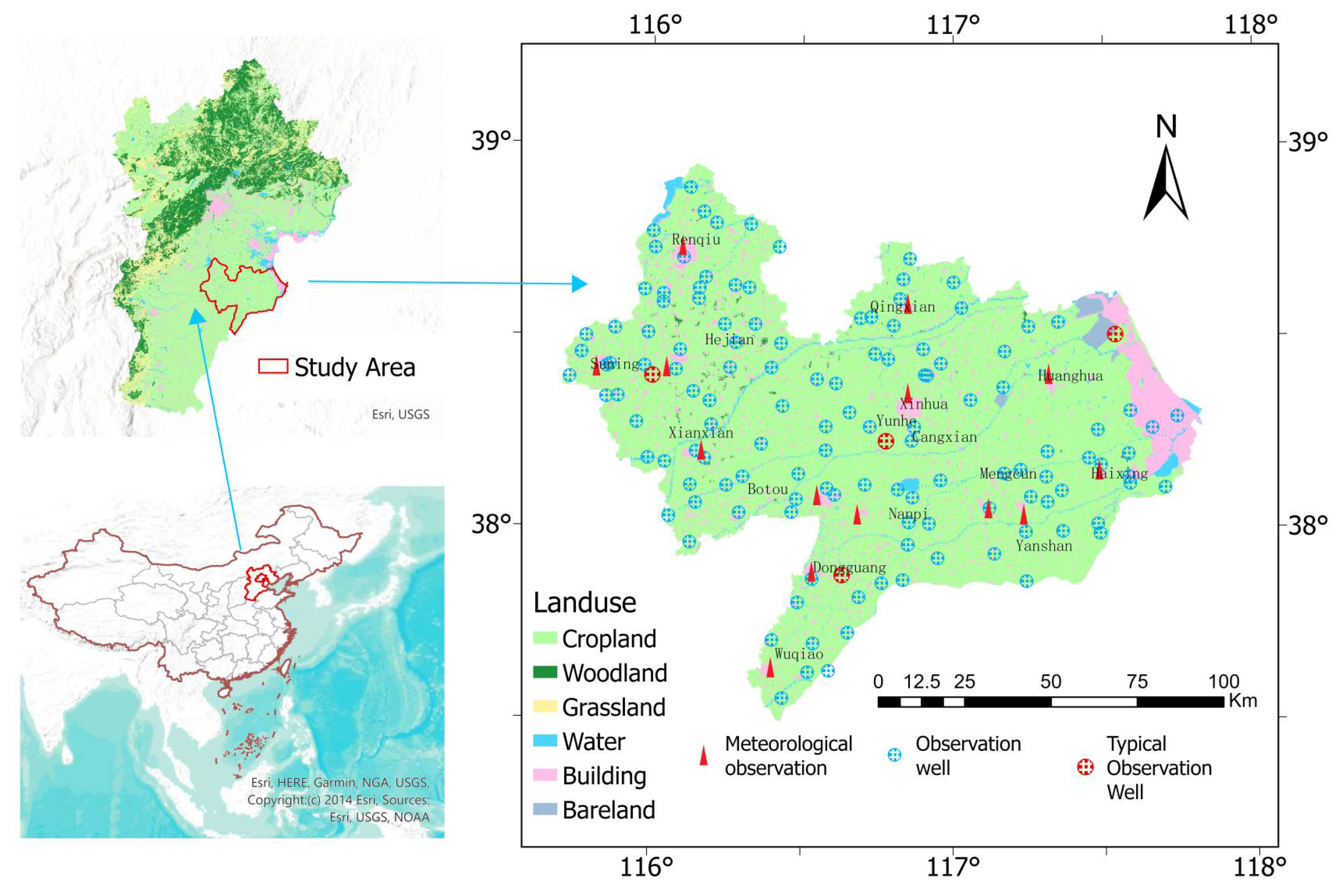
Cangzhou is located along the Bohai Bay coast in southeastern Hebei Province and has a warm temperate, semi-humid continental monsoon climate. With an average annual precipitation of around 500 mm, the region suffers from limited surface water resources and elevated salinity levels in shallow groundwater. As a result, agricultural production in Cangzhou relies heavily on the extraction of deep groundwater. Influenced by monsoonal patterns, the temporal and spatial distribution of precipitation is highly uneven, significantly misaligned with the water demand cycle of major crops, such as wheat and corn. This imbalance has resulted in severe overextraction of groundwater and the development of a large-scale regional cone of depression. In the central part of the region, groundwater levels have dropped to below −90 m. The South-to-North Water Diversion Project (SNWDP) is China’s largest inter-basin water transfer initiative, designed to mitigate the uneven distribution of water resources between the north and south. Since the launch of the Middle Route in 2017, Cangzhou—one of the project’s receiving regions—has received approximately 453 million cubic meters of water annually from the Yangtze River. This external supply has been used to reduce reliance on deep groundwater extraction. As a result, groundwater levels in the region have begun to recover. By 2022, the deep groundwater level in Cangzhou had risen by 2.8 m compared to 2017 [18].

Figure 1 illustrates the spatial distribution of land use types, groundwater observation wells, and meteorological stations across the Cangzhou region. Among the observation wells, four representative wells were selected as typical monitoring points for further analysis. As shown in the figure, most wells are located in cropland areas, highlighting the region’s dominant agricultural land use. A smaller number of wells are situated within built-up areas, while only a few are located near grasslands, woodlands, water bodies, or bare land. This distribution pattern suggests that the monitoring network is predominantly situated within agricultural landscapes. As a result, it offers a solid data foundation for analyzing groundwater dynamics under agricultural land use and their interactions with meteorological factors.

This land use dataset was based on Landsat satellite imagery and interpreted through manual visual interpretation. It adopts a hierarchical classification system, including six primary land use categories.

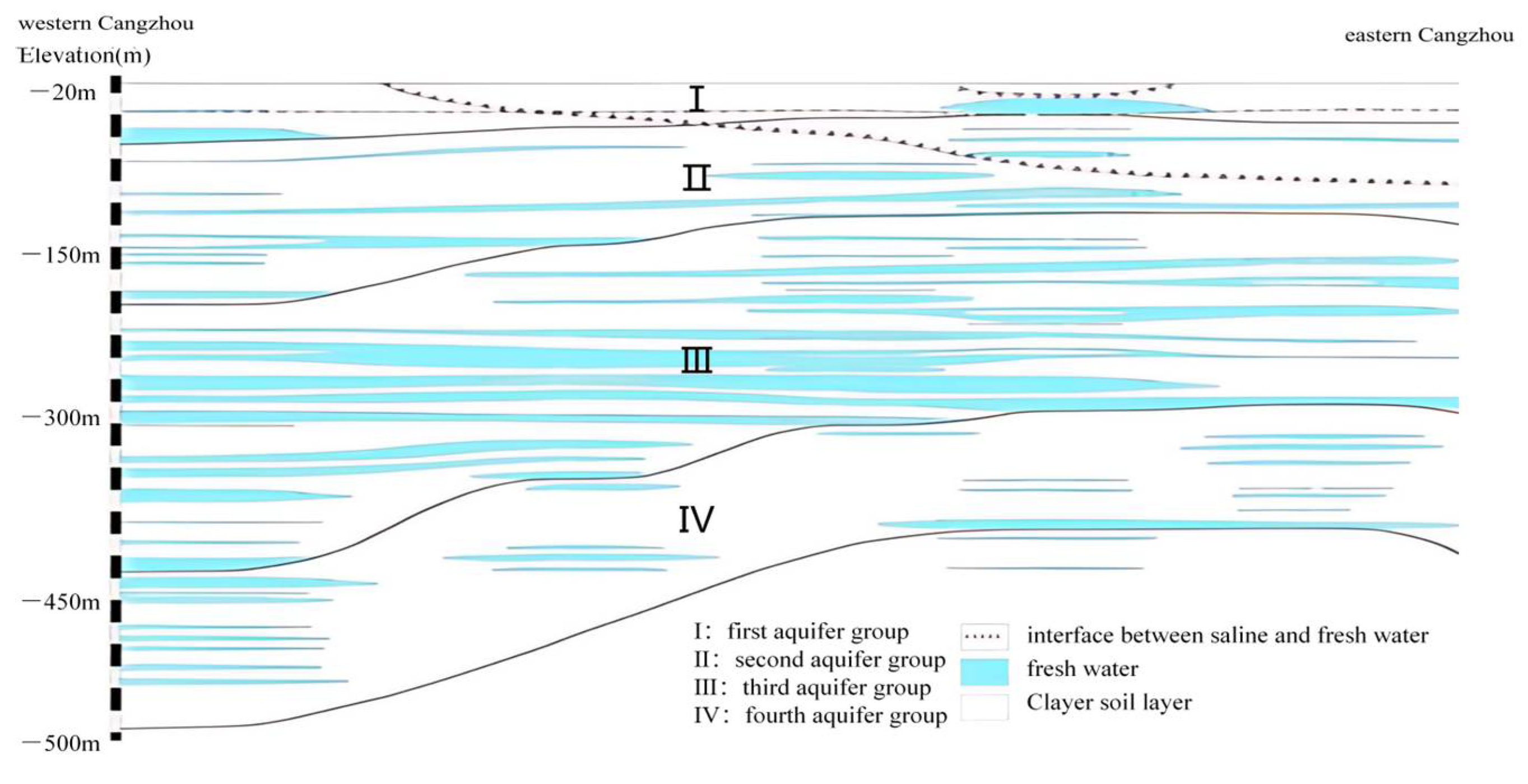
The hydrogeological structure of the study area exhibits distinct vertical stratification. The Quaternary aquifer system can be subdivided into four aquifer units from top to bottom, each with distinct hydraulic properties. The first aquifer unit is a shallow unconfined aquifer directly recharged by atmospheric precipitation, with individual well discharge rates ranging from 8 to 20 m³/h. Water quality in this layer transitions gradually from fresh to slightly brackish as one moves from west to east. The second aquifer unit is confined and located at depths of 120–220 m. It is overlain by a stable aquiclude, which significantly limits lateral recharge. The third aquifer unit, currently the primary target for groundwater extraction, lies at depths of 250–420 m and consists mainly of alluvial fine sands. This unit supports high discharge rates (20–80 m³/h) and generally contains groundwater with mineralization levels below 2 g/L, offering both high yield and good water quality. The fourth aquifer unit is found below approximately 380 m and is characterized by markedly reduced permeability and a low unit yield of only 1.0–1.5 m³/h, thus representing the least favorable recharge conditions. Owing to its superior water quality and high productivity, the third aquifer unit serves as the main exploitation layer in the study area [19]. The specific zoning is shown in Figure 2 (adapted from the Hydrogeological Report of Cangzhou City).

3. Methodology

3.1. Feature Relevance Analysis

3.1.1. Pearson Correlation Coefficient

As a classic tool for measuring linear correlation, the Pearson correlation coefficient (PCC) is widely used in feature autocorrelation analysis [20]. It is mathematically defined as the normalized ratio of the covariance to the product of the standard deviations of two random variables. The specific expression is as follows:

$$\rho \left(X,X_T\right)={\displaystyle \frac{E\left[\left(X_t-{\mu }_X\right)\left(X_{t-T}-{\mu }_X\right)\right]}{{\sigma }_X\cdot {\sigma }_{X_T}}}.$$

(1)

In the formula, $X_t$ represents the observed value of the time series at time $t$, $X_{t-T}$, $T$ is the observed value lagged by $T$ periods, ${\mu }_X$ is the expected value of the sequence, and ${\sigma }_X$ is the standard deviation. The coefficient ranges from [−1, 1], where a value of 1 indicates perfect positive autocorrelation, a value of −1 indicates perfect negative autocorrelation, and a value of 0 indicates no linear autocorrelation.

3.1.2. Mutual Information

In order to capture nonlinear correlations that the Pearson coefficient may overlook, this study further incorporated mutual information (MI) as a complementary method for evaluating the relevance between features and groundwater levels.

As an information-theoretic metric, mutual information (MI) is increasingly used in feature relevance analysis due to its ability to detect both linear and nonlinear relationships between variables. Unlike Pearson correlation, which only captures linear dependencies, mutual information quantifies the amount of information obtained about one random variable through observing another. It is especially suitable for groundwater prediction problems involving complex interactions between climatic, anthropogenic, and geospatial factors [21].

Mathematically, mutual information between two random variables $X$ and $Y$ is defined as follows:

$$MI(X,Y)={\displaystyle \sum _{x\in X}{\displaystyle \sum _{y\in Y}p(x,y)\log \left(\frac{p\left(x,y\right)}{p\left(x\right)p\left(y\right)}\right)}},$$

(2)

where $p(x,y)$ is the joint probability distribution of $X$ and $Y$, while $p\left(x\right)$ and $p\left(y\right)$ are the marginal probability distributions of $X$ and $Y$, respectively. When $X$ and $Y$ are statistically independent, $MI\left(X,Y\right)=0$. The larger the mutual information value, the stronger the dependency between variables.

This method is capable of capturing the complex, nonlinear relationships commonly observed in groundwater systems—such as lagged recharge effects and threshold-type responses. Compared to traditional linear correlation analysis, it offers a more comprehensive and physically meaningful criterion for variable selection.

Figure 3 shows a two-stage feature selection workflow combining Pearson correlation analysis and mutual information (MI). In the first stage, pairwise Pearson correlation coefficients were calculated to identify and remove linearly redundant features (i.e., if the absolute correlation between two features exceeds 0.6, one is retained and the other is discarded). In the second stage, MI scores were computed between each remaining feature and the target variable (groundwater level). Features with MI values lower than one-fifth of the median MI score were eliminated. The final selected feature subset was used as input for model training.

3.2. Introduction to Stacking Ensemble Learning

Stacked generalization, commonly known as Stacking, was proposed as a higher-order ensemble learning method [22]. Its core concept is to construct a hierarchical model architecture, where the outputs of multiple base learners serve as input features for a meta-learner. This design facilitates the collaborative optimization of heterogeneous models [23]. Compared with traditional ensemble methods, Stacking introduces a meta-learning mechanism that significantly enhances both generalization performance and prediction accuracy. The Stacking process operates in two stages.

At the base level, NNN heterogeneous learners—such as decision trees, support vector machines, and neural networks—are independently trained on the same dataset to produce predictions. These models are often specialized in handling different data structures or feature types, and their combination allows for leveraging their individual strengths. At the meta level, the predictions from the base learners are treated as a new feature space. A meta-learner is then trained on this transformed dataset to produce the final ensemble output [24]. Figure 4 illustrates the relevant process of this learning model.

To avoid the overfitting problem caused by using the same training set for both the base learner and the meta-learner, Stacking employs K-fold cross-validation to generate meta-features. Specifically, the original training set D is divided into K mutually exclusive subsets $\left\{D_1,D_2,\cdots D_i\right\}$. For the i-th fold, the base learner is trained using $D/D_i$, training the base learner $C_j$(j = 1, 2, ……N). Then, $D_i$ is input into $C_j$ to generate the prediction result $P_j$, the k-fold prediction results are concatenated into a meta-feature matrix $P=\left[P_1,P_2\cdots P_N\right]$, and the meta-learner is jointly trained with the original label y. The specific process is shown in Figure 5.

3.3. Data Sources and Processing

Due to meteorological factors and artificial exploitation being the main influencing factors of groundwater level changes, precipitation (PRE), air temperature (TEM), atmospheric pressure (PRS), wind speed (WIND), relative humidity (RHU), and extraction volume (EXTRACT) were selected as characteristic variables [25]. Considering that the lagged groundwater levels (La-GWLs) from the same period of the previous year can effectively capture seasonal fluctuations and inter-annual variation patterns, they were incorporated as feature variables to enhance the model’s ability to represent periodic dynamics [26]. Additionally, recognizing the significant spatial heterogeneity of groundwater levels, land use types (LU) and ground elevation were incorporated as model characteristic variables [27]. Ground elevation data with a spatial resolution of 1 km were derived from the digital elevation model (DEM). All input features and corresponding response variables were divided into 2018–2021 data for training, with 2022 data used for testing the Stacking ensemble learning model and other base learner models.

3.3.1. Data Source

We collected monthly groundwater level monitoring data from 131 third-aquifer-layer monitoring wells within Cangzhou City from 2017 to 2022, along with monthly electricity consumption data (used to estimate groundwater extraction) from over 52,400 pumping wells in the same area during 2018–2022. Kernel density analysis was applied to calculate the electricity consumption (i.e., extraction intensity) of pumping wells surrounding each monitoring well (groundwater extraction data provided by Cangzhou Water Resources Bureau). Meteorological data near monitoring wells were obtained through Kriging interpolation using observations from 14 national-level meteorological stations in the Cangzhou region (data.cma.cn) [28]. Ground elevation and land use type raster data were acquired from the National Natural Resources Science Data Platform (www.resdc.cn) [29].

Table 1. Data sources of feature variables.

Category	Variable	Description	Source
Climate	Temperature	Monthly average temperature (°C)	National Meteorological Monitoring Stations
	Precipitation	Monthly average precipitation (mm)
	Air Pressure	Monthly average air pressure (pa)
	Wind Speed	Monthly average wind speed (m/s)
	Relative Humidity	Monthly average relative humidity (%)
Spatial Geographic Information	Ground Elevation	Altitude value (m)	Natural Environment Science Data Platform
	Land Use Type	Crop land, woodland, etc.
Human Activities	Extraction Volume	Monthly average mining electricity consumption (kWh)	Cangzhou Water Affairs Bureau

shows the sources of the aforementioned data.

Additionally, the annual water transfer volumes from the South-to-North Water Diversion Project (SNWDP) to Cangzhou between 2018 and 2022 were compiled, as presented in

Table 2. The water diversion volume of the South-to-North Water Diversion Project and the extraction volume of deep groundwater (million cubic meters).

Year	2018	2019	2020	2021	2022
Extraction	38,515.08	26,307.8	20,440	12,159.5	11,758.5
Water diverted	26,909	28,662	32,100	36,511	51,481
Total	65,424.08	54,969.8	52,540	48,670.5	63,239.5

. In a counterfactual scenario where no SNWDP water allocation is provided, and considering that shallow unconfined groundwater in most areas of Cangzhou is brackish and unsuitable for direct use, the resulting water deficit for industrial, domestic, and agricultural needs would have to be compensated through increased extraction of deep groundwater. Based on this assumption, the estimated electricity consumption for groundwater pumping under such a water-stressed scenario was calculated by determining the ratio between total water demand (in the absence of SNWDP supply) and the actual recorded groundwater extraction volume.

So, under the scenario without SNWDP supply, the groundwater pumping electricity consumption for each well was calculated using the following formula:

$$E{c}_1=E{c}_{actual}\times (deficit/V_{actual}),$$

(3)

$$deficit=V_{actual}+V_{transfer},$$

(4)

where $E{c}_1$ is the energy consumption of groundwater extraction under the scenario without the South-to-North Water Diversion Project, $E{c}_{actual}$ is the actual energy consumption of groundwater extraction, $V_{actual}$ is the actual volume of groundwater extracted, $deficit$ represents the water resource deficit, and $V_{transfer}$ is the volume of water transferred through the South-to-North Water Diversion Project.

3.3.2. Data Preprocessing

This study adopted a rigorous data preprocessing protocol to ensure analytical quality. During outlier treatment, a dual verification process was initially employed combining boxplot analysis with the 3-sigma rule. Specifically, by calculating the first quartile $Q_1$ and third quartile $Q_3$ values, the interquartile range $IQR\left(Q_3-Q_1\right)$ was determined. Outliers were identified as data points exceeding the thresholds of $[Q_1-1.5\times IQR,Q_3+1.5\times IQR]$. Data points that fell outside the specified range were identified as outliers and subsequently removed. This standard can effectively identify extreme values that deviate from the overall distribution pattern. For missing data, a regression model based on variable correlation was constructed to perform imputation. For example, a regression equation can be established with the completely observed groundwater level data as the independent variable and the missing water level data as the dependent variable. Data imputation was achieved through model prediction, which not only preserved the inherent correlation characteristics among variables but also avoided biases resulting from simple interpolation. The processing flow is shown in Figure 6.

3.4. Predictive Model Framework

Figure 7 illustrates the model prediction framework, which involved the following steps.

For each monitoring well, La-GWL, EXTRACT, PRE, Wind, LU, and DEM were selected as feature variables for forecasting groundwater levels (GWLs). Based on the results of the correlation analysis, TEM, PRS, and RHU were excluded due to their weak relevance. The final groundwater level forecasting model was expressed mathematically, as shown in Equation (5):

$$GW{L}_{t,i}=f\left(DE{M}_{t,i},EXTRAC{T}_{t,i},L{U}_{t,i}La-GW{L}_{t,i},PR{E}_{t,i},WIN{D}_{t,i}\right),$$

(5)

where $DEM$ represents the ground elevation, $EXTRACT$ denotes the extraction volume, $La-GWL$ stands for the lagged groundwater level from the same period of the previous year, $PRE$ indicates precipitation, $WIND$ signifies wind speed, $t$ represents time, and $i$ denotes the $i\mathrm{th}$ monitoring well.

3.4.1. Introduction to Base Learners

To construct a high-performance ensemble prediction model, six representative machine learning algorithms were selected as base learners. These algorithms span various categories, including instance-based learning, neural networks, ensemble learning, and kernel methods. Each base model offers distinct advantages in handling nonlinear relationships, high-dimensional inputs, and time series data, thereby contributing diverse learning representations to the Stacking ensemble framework.

Table 3. Introduction to base learners.

Algorithm	Category	Core Mechanism	Reference
KNN	Instance-based non-parametric model	Weighted voting through sample distance calculation	[30]
MLP	Feedforward neural network	Stacked fully connected layers + nonlinear activation functions	[31]
CNN	Deep learning model	Convolutional layers for spatial/temporal feature extraction + pooling + nonlinearity	[32]
RF	Ensemble learning (Bagging)	Parallel training of multiple decision trees + bootstrap sampling + random feature subsets	[33]
XG-Boost	Ensemble learning (Boosting)	Gradient-boosted trees + second-order derivative optimization + regularization	[34]
SVR	Kernel method model	Constructs optimal hyperplane in high-dimensional space + insensitive loss function	[35]

summarizes the algorithm category, core mechanism, and relevant references for each base learner, providing theoretical and technical support for the model integration process.

3.4.2. Construction of Meta-Learner

The meta-learner was redesigned as a weighted average mechanism, and it now directly computes predictions through a learnable weighted combination of base learners:

a.

Input Layer: Accepts predictions from 6 base learners (matching the original count).

b.

Weighting Layer: Assigns a trainable weight to each base learner’s prediction. These weights are initialized equally (e.g., 1/6 for uniform starting importance) and optimized during training.

c.

Output: The final water level prediction is generated by aggregating the weighted base predictions using a linear combination (sum of products between weights and base predictions). No activation function is applied to ensure unconstrained regression output.

The process of the meta-learner is illustrated in Figure 8.

3.4.3. Model Evaluation Metrics

To evaluate the prediction accuracy of different models, MAE (mean absolute error), RMSE (root mean squared error), and R² (coefficient of determination) were used as the evaluation metrics for the models:

$$\mathrm{MAE}={\displaystyle \frac{1}{n}}{\displaystyle \sum _{i=1}^n\left|y_i-{\widehat{y}}_i\right|},$$

(6)

$$\mathrm{RMSE}={\displaystyle \frac{1}{n}}{\displaystyle \sum _{i=1}^n{\left(y_i-{\widehat{y}}_i\right)}^2},$$

(7)

$$R^2=1-{\displaystyle \frac{{\displaystyle \sum _{i=1}^n{\left(y_i-{\widehat{y}}_i\right)}^2}}{{\displaystyle \sum _{i=1}^n{\left(y_i-{\overline{y}}_i\right)}^2}}},$$

(8)

where $y_i$ is the actual observed groundwater level, ${\widehat{y}}_i$ is the model predicted value, $\overline{y}$ is the average of all observations, and $n$ is the number of samples. The closer RMSE and MAE are to 0, and the closer $R^2$ is to 1, the more accurate the prediction result is.

3.5. Feature Importance Analysis

Conducting feature importance analysis after model training offers a key advantage: it enables an in-depth examination of how individual features contribute to prediction outcomes, based on the internal characteristics of the trained model [36]. By employing advanced interpretation tools, such as SHAP values, we can quantify the marginal contribution of each feature to the model output, accurately identify key features, optimize the model structure, or adjust feature selection strategies, thereby enhancing the model’s generalization ability and practical application value.

SHAP is based on the Shapley value in game theory, which fairly allocates the contribution of each feature to the prediction result. For a regression model f, the predicted value f(x) for a sample x can be decomposed as:

$$f\left(x\right)={\phi }_0+{\displaystyle \sum _{j=1}^p{\phi }_j}.$$

(9)

In the formula, ${\phi }_0$ represents the baseline prediction (the mean of the target variable in the training set, $E\left[y\right]$) and ${\phi }_j$ is the SHAP value for feature $j$, and its calculation formula is:

$${\phi }_j={\displaystyle \sum _{S\subseteq (1,\cdots p)/\left\{j\right\}}\frac{\left|S\right|!\left(p-\left|S\right|-1\right)!}{p!}}\left[f\left(S\cup \left\{j\right\}\right)-f\left(S\right)\right].$$

(10)

In the formula, $S$ is a subset of features, $p$ is the total number of features, and $f\left(S\right)$ is the model prediction value using subset $S$.

We calculated the SHAP value matrix $\varphi \in R^{n\times p}$ for all samples, computed the global importance scores, and sorted them by the mean of the absolute SHAP values of features:

$$Global Importanc{e}_j={\displaystyle \frac{1}{n}}{\displaystyle \sum _{i=1}^n\left|{\varphi }_j^i\right|}.$$

(11)

4. Results

This section provides a comprehensive evaluation of model performance and offers an in-depth analysis of the Stacking ensemble strategy in the context of groundwater level forecasting.

The analysis focused on four key aspects:

(1)

overall predictive performance across different models,

(2)

single-well performance under spatially heterogeneous hydrogeological conditions,

(3)

error analysis from both statistical and spatiotemporal perspectives, and

(4)

interpretation of feature importance.

Visual and quantitative comparisons demonstrated that the Stacking ensemble model consistently outperformed individual base learners in terms of accuracy, robustness, and generalization. Its superior performance is primarily attributed to its ability to integrate the complementary strengths of diverse algorithms while mitigating the limitations inherent in single models.

The following subsections aim to explain not only the predictive performance of the model but also the underlying mechanisms that drive its effectiveness. This dual focus provides deeper insights into the reliability and applicability of the proposed approach in complex, multi-factor groundwater systems.

4.1. Feature Relevance Analysis

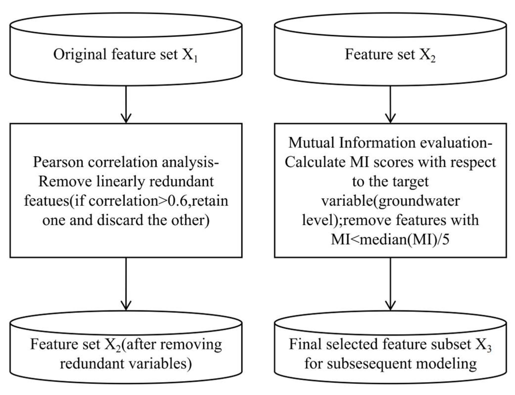
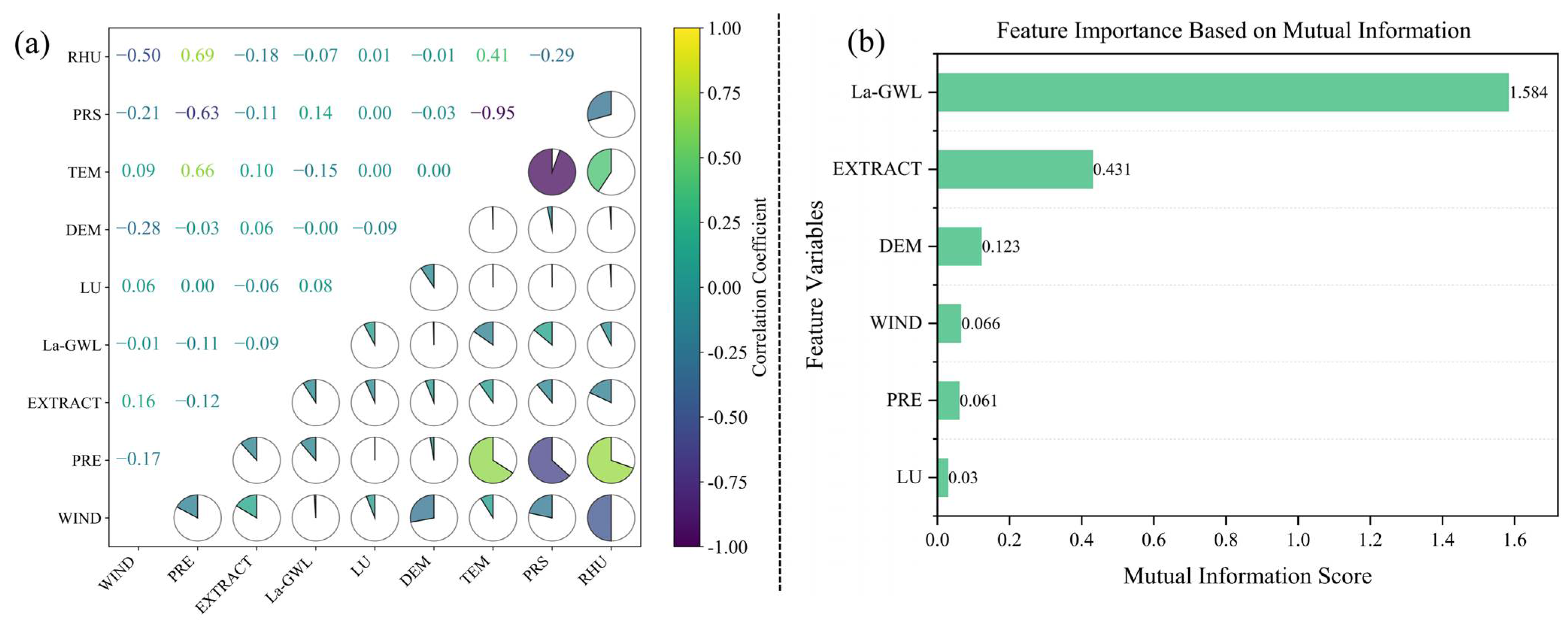
To improve model interpretability and reduce feature redundancy, a two-stage feature selection process was applied based on the Pearson correlation coefficient and mutual information (MI). Figure 9a,b present the outcomes derived from the Pearson correlation coefficient and mutual information analyses, respectively.

In the first stage, the Pearson correlation matrix was used to identify feature pairs with high linear correlation (|PCC| > 0.6). Strong correlations were observed between several meteorological features, including rainfall–pressure, rainfall–relative humidity, rainfall–temperature, and pressure–relative humidity. Based on the established criterion, one variable from each highly correlated pair was removed. Given the direct hydrological impact of rainfall on groundwater recharge, rainfall was retained, while pressure, temperature, and relative humidity were excluded.

In the second stage, mutual information scores were computed between each remaining feature and the target variable (groundwater level) to assess their nonlinear relationships. All retained features showed MI scores above one-fifth of the median threshold, indicating their substantial contribution to groundwater level prediction. As a result, no further features were excluded at this stage.

Following the two-stage screening, the final selected features included rainfall, wind speed, groundwater extraction volume, land use type, lagged groundwater level, and surface elevation, which were subsequently used as model inputs.

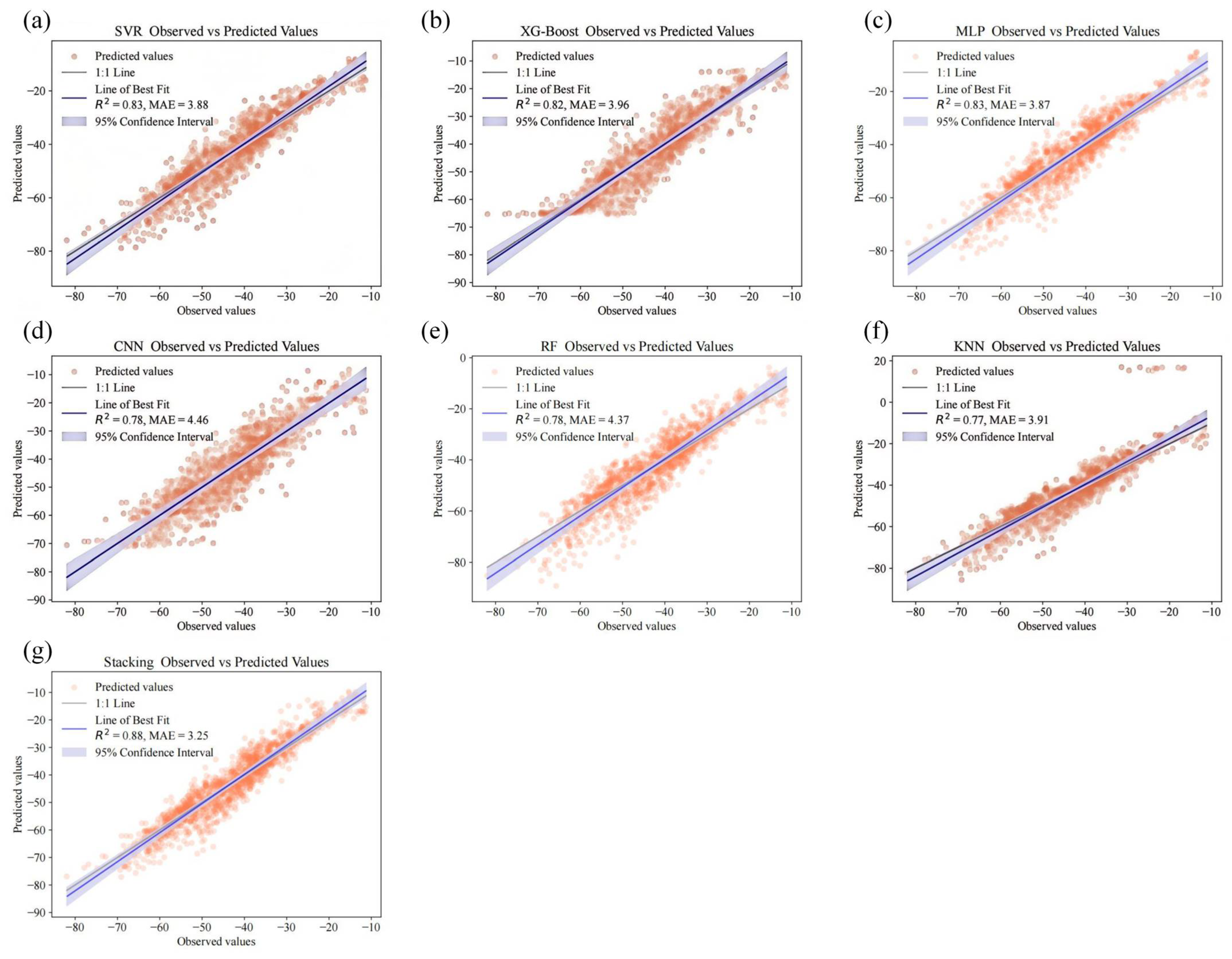
4.2. Overall Prediction Performance

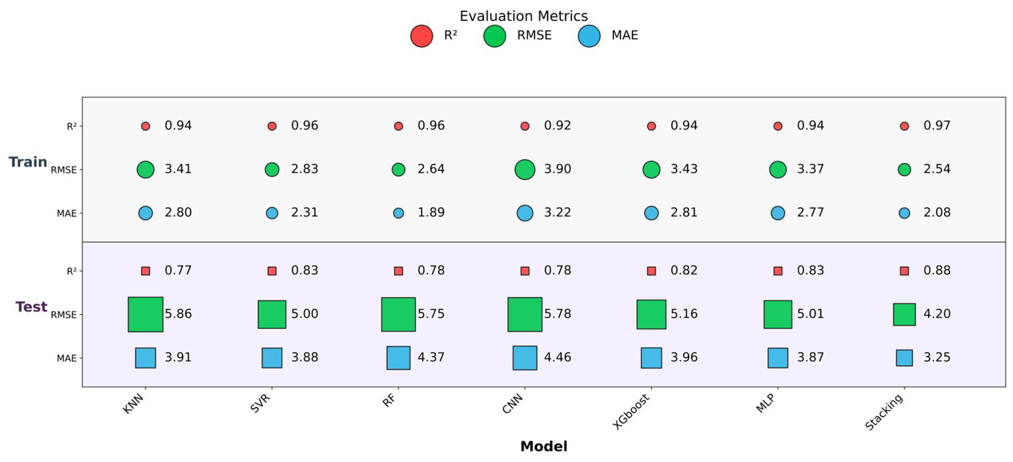
A comprehensive evaluation of model performance (Figure 10) highlighted the superior predictive ability of the Stacking ensemble model over individual base learners. In the scatter plot comparing observed and predicted groundwater levels, the Stacking model’s predictions exhibited a tighter clustering along the 1:1 reference line, indicating a stronger agreement between predicted and actual values. This visual correspondence was further corroborated by quantitative evaluation metrics (Figure 11), where the ensemble model consistently outperformed its individual components across all indicators.

Specifically, on the test set, the Stacking model achieved an MAE of 3.25 m and RMSE of 4.20 m, representing a reduction of 16.2% and 16.0%, respectively, compared to the best-performing individual model (SVR). Furthermore, the R² value increased from 0.83 (MLP) to 0.88, demonstrating a marked improvement in the explained variance. These improvements suggest that the ensemble model not only enhanced accuracy but also achieved better generalization performance on unseen data.

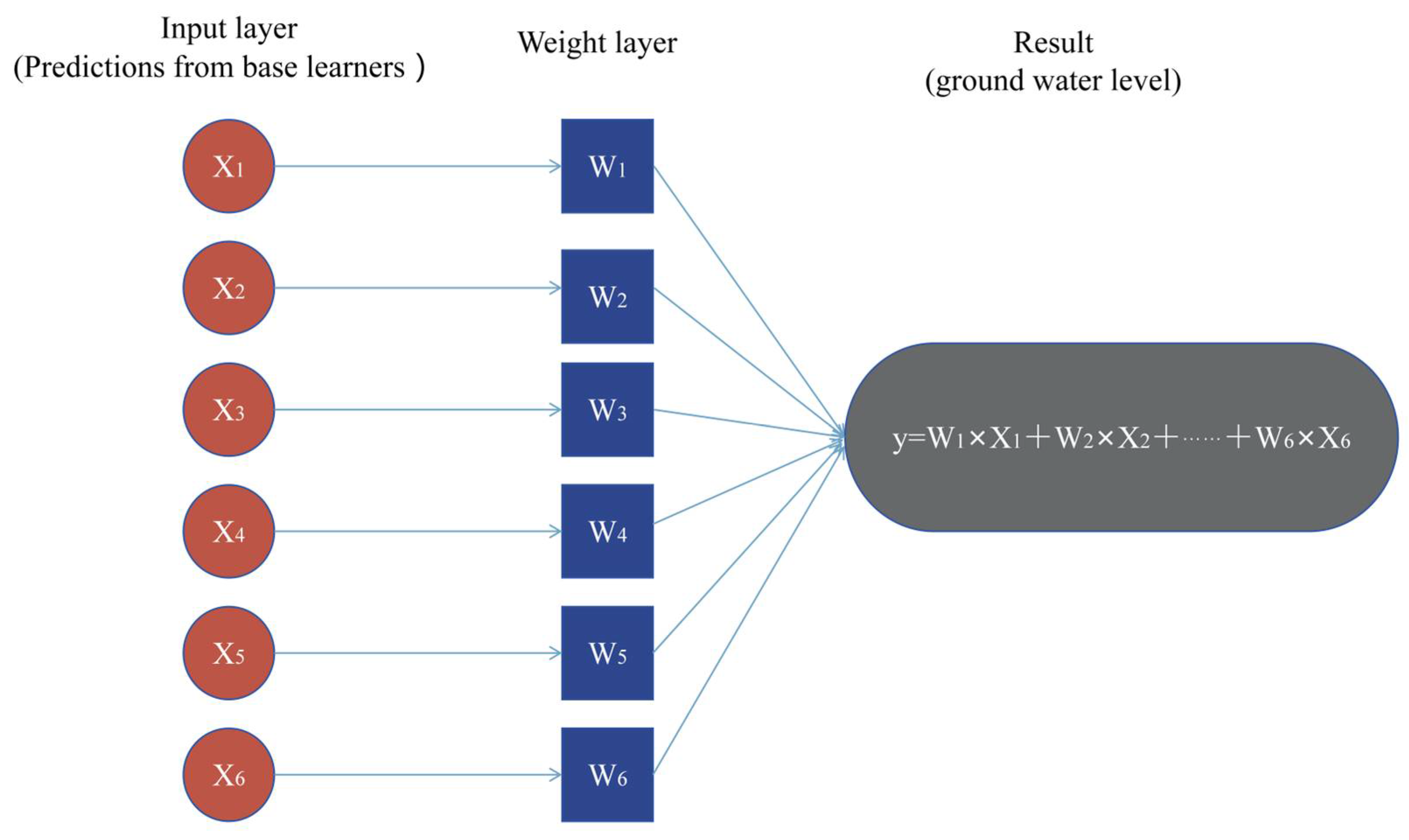
The improved performance of the Stacking model can be attributed to its ability to integrate complementary strengths of heterogeneous base learners, including KNN, CNN, RF, SVR, XG-Boost, and MLP. For example, while tree-based methods (RF and XG-Boost) are effective in capturing nonlinear relationships and handling variable importance, models like CNN and MLP excel at recognizing complex patterns in high-dimensional spaces. The Stacking strategy leverages these diverse modeling perspectives by assigning optimized weights through a meta-learner—here, a weighted average approach—which effectively balances the prediction biases and variances of individual models.

Another critical advantage of the Stacking framework lies in its robustness to overfitting. Unlike individual learners that may tailor closely to specific features or patterns in the training set (e.g., CNN’s sensitivity to spatial correlations), the ensemble mitigates such tendencies by aggregating multiple decision boundaries. This was evident in the consistent superiority of Stacking across both training and test sets, suggesting that the model not only fit the training data well but also maintained predictive reliability under varying input conditions.

In summary, the Stacking ensemble model demonstrated significant advantages over standalone algorithms in terms of both predictive accuracy and generalization ability. Its performance benefits arose from its integrative architecture, which effectively fused the complementary modeling capabilities of diverse learners and mitigated the limitations of any single model. This confirmed the suitability of ensemble learning, particularly Stacking, as a powerful approach for groundwater level prediction in complex, multi-factor environments.

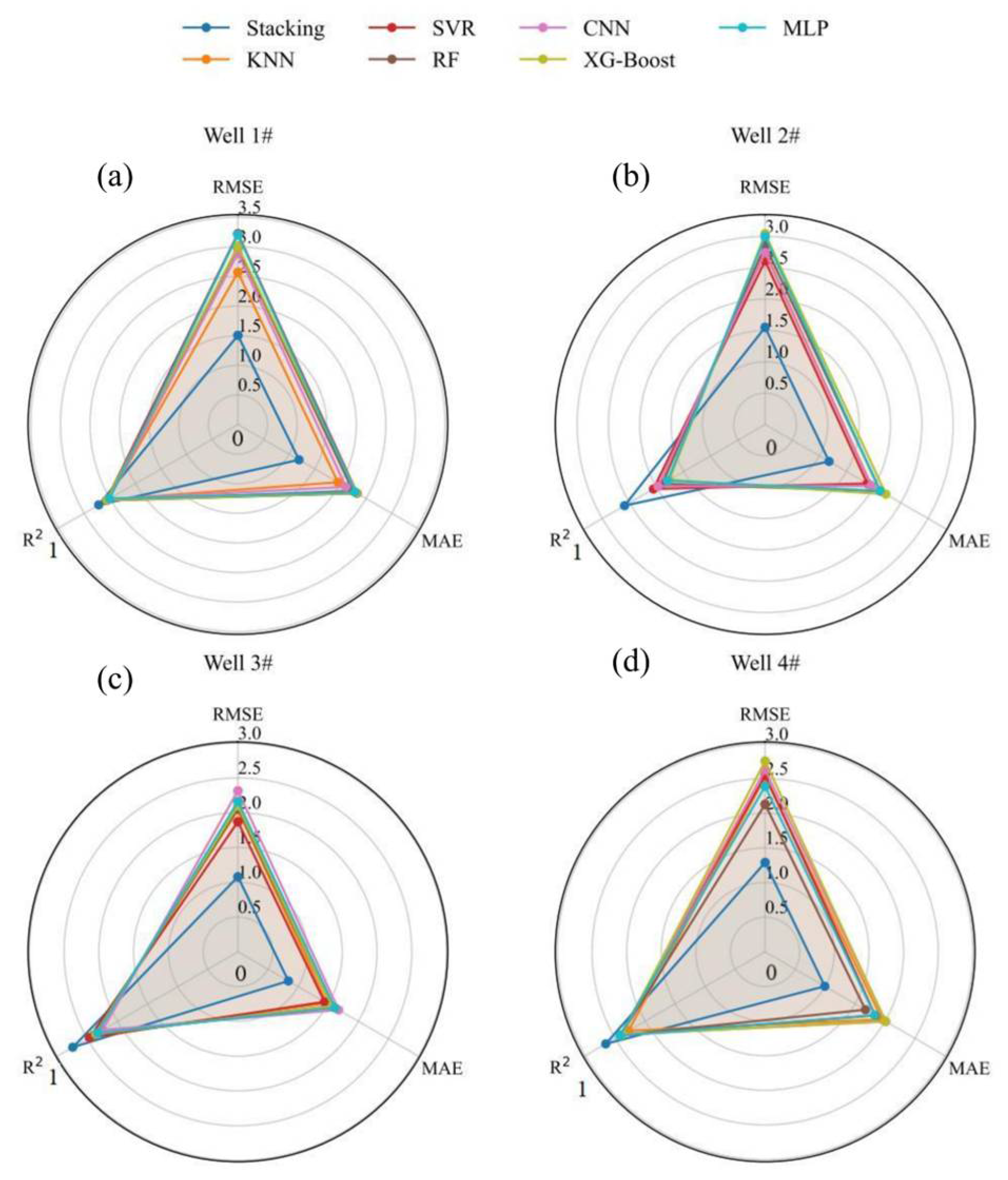
4.3. Well-Level Performance in Heterogeneous Aquifers

To further evaluate the generalization capability of the proposed Stacking ensemble model under varying hydrogeological conditions, this study conducted a single-well analysis based on four representative observation wells distributed across spatially heterogeneous regions. These wells were selected to capture diverse aquifer characteristics, including variations in lithology, groundwater depth, and anthropogenic influence. By comparing the prediction performance at each well, we aimed to assess the local adaptability and robustness of the Stacking framework relative to individual learning algorithms.

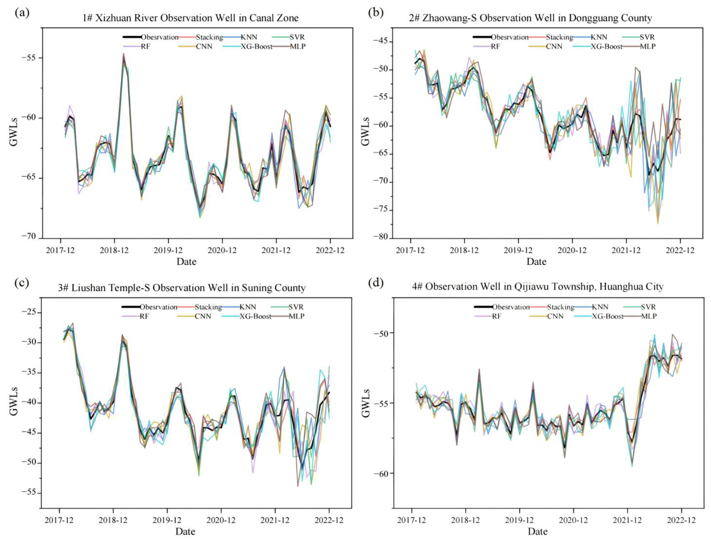
As shown in Figure 12, the Stacking ensemble consistently achieved superior prediction accuracy across all selected wells, outperforming baseline models, such as CNN, KNN, SVR, RF, XG-Boost, and MLP, in terms of RMSE, MAE, and R². Specifically, the ensemble model achieved RMSE values ranging from 1.08 m to 2.08 m and MAE values between 0.52 m and 1.54 m, reflecting reductions of 34–66% and 28–49%, respectively, when compared to the best-performing individual learners. Furthermore, the coefficient of determination (R²) ranged from 0.76 to 0.83, representing an improvement of 12–60% over the standalone models. As illustrated in Figure 13, the prediction results of the Stacking ensemble model exhibit closer alignment with observed outcomes compared to alternative models.

This consistent performance advantage across spatially distinct wells highlighted several important attributes of the Stacking model. First, its ensemble architecture enabled the integration of diverse base learners with complementary modeling capabilities. For instance, CNN and MLP are adept at capturing high-dimensional and nonlinear patterns, while tree-based models like RF and XG-Boost excel at handling feature interactions and noise robustness. The meta-learner, implemented as a weighted average in this study, dynamically balanced the contributions of these base learners based on their local strengths, thus enhancing the model’s adaptability to varying geological settings.

Second, the superior generalization performance of the Stacking model is particularly notable given the pronounced heterogeneity in aquifer conditions. In individual models, performance is often sensitive to local data characteristics—for example, KNN may struggle in sparsely sampled wells, and SVR may be less robust to outliers or non-stationary inputs. By contrast, the ensemble approach mitigated such model-specific weaknesses, yielding more stable predictions across different wells.

In summary, the single-well analysis reinforced the conclusion that the Stacking ensemble learning model is not only accurate on a global scale but also robust and adaptable under localized hydrogeological variability. This makes it particularly suitable for groundwater prediction tasks in regions with complex spatial heterogeneity, where single-model solutions often fall short.

4.4. Error Analysis: Distribution Structure and Spatiotemporal Deviations

To further evaluate the reliability and robustness of the Stacking ensemble learning model, a detailed residual analysis was performed using prediction errors—defined as the differences between predicted and observed groundwater levels on the test set.

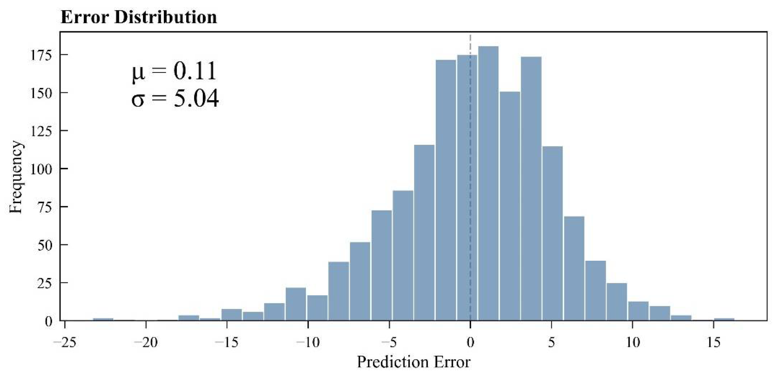
As shown in Figure 14, the histogram of residuals closely approximated a symmetric bell-shaped distribution. The Shapiro–Wilk normality test (p > 0.05) confirmed that the residuals did not significantly deviate from normality, indicating that the model’s overall error structure was statistically stable and well-behaved.

Two key insights emerged from the residual statistics. First, the residual mean was slightly positive (+0.11 m), indicating a mild systematic overestimation. This bias may stem from an uneven distribution of high-value samples in the training set or insufficient regularization in certain base learners (e.g., CNN), leading to minor overfitting in high groundwater level ranges. Second, the 95% confidence interval spanned from −9.76 m to +9.98 m, suggesting that the vast majority of errors fell within ±10 m—well within the acceptable range for practical groundwater management and engineering applications.

It should also be noted that the data used in this study spanned only from 2018 to 2022, as the groundwater monitoring network in the study area was not fully established until 2018. Prior to that, the number of monitoring stations was limited, and continuous, reliable data were unavailable. Although the use of lagged groundwater levels and monthly cumulative sequences helped mitigate this limitation, the relatively short time span may still affect the model’s ability to capture long-term trends, such as climate variability or cumulative overextraction. With the continuous accumulation of monitoring data in the future, the model can be further improved, and prediction errors are expected to decrease accordingly.

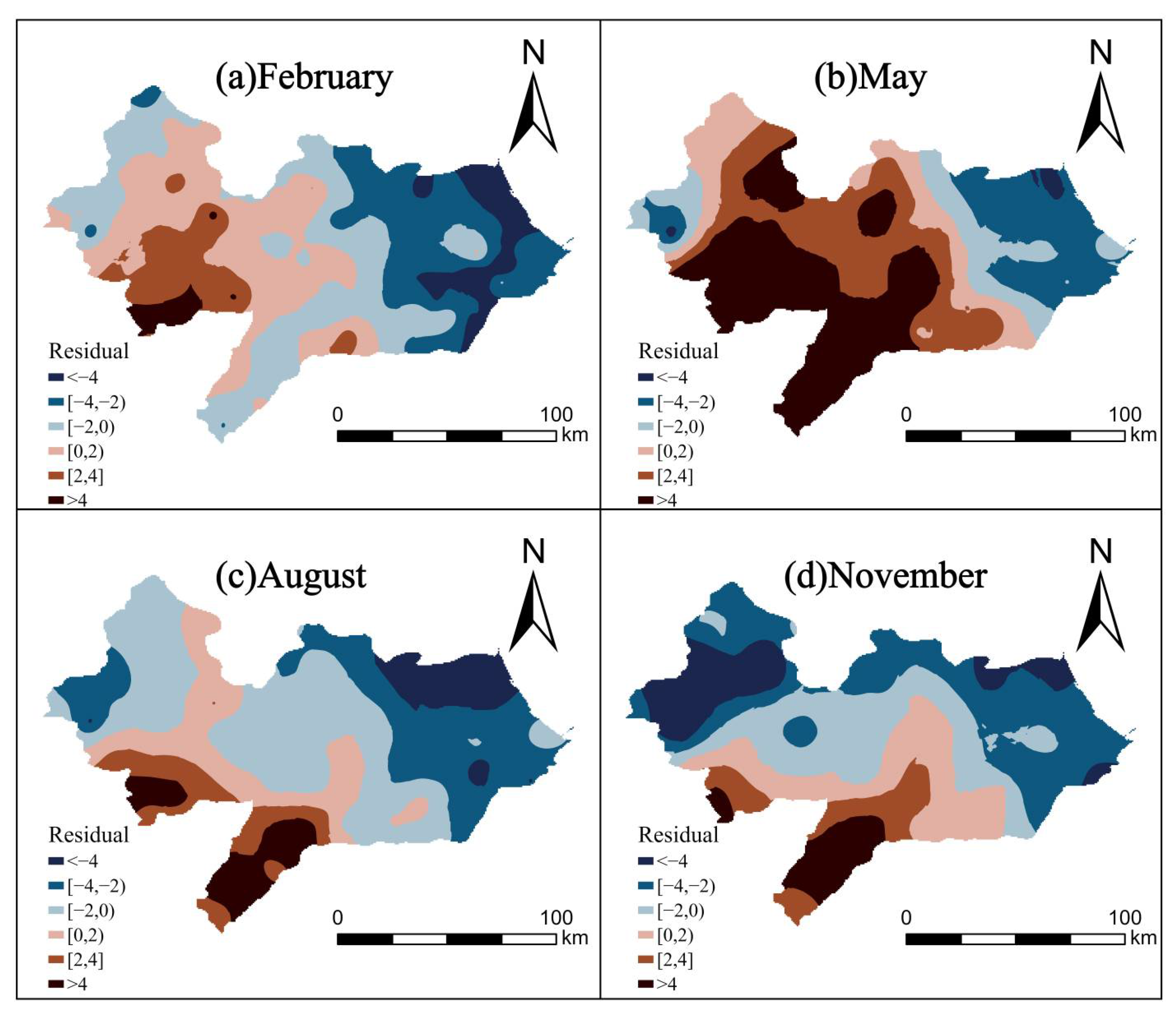
To examine the spatiotemporal distribution of prediction errors, a residual map was generated for the test set (Figure 15). Spatial analysis revealed notable regional variation: predictions in southern Cangzhou tended to be slightly overestimated, while those in the western and eastern regions tended to be underestimated. These spatially systematic errors may reflect underlying hydrogeological heterogeneity. For example, the southern region may have higher hydraulic conductivity or better aquifer connectivity, enabling faster recovery of groundwater levels following recharge or reduced extraction—dynamics that may not be fully captured by the current feature set.

In contrast, the western and eastern areas may be characterized by lower transmissivity or more confined aquifer conditions, leading to slower recovery and underestimation by the model. Moreover, spatial heterogeneity in extraction intensity—such as concentrated agricultural groundwater extraction in specific zones—can further impact prediction accuracy if not adequately represented in spatial features. These findings suggest that future model improvements may benefit from incorporating detailed geological cross-sections, borehole profiles, and high-resolution groundwater extraction records to account for localized hydrogeological variability.

In summary, the residual analysis confirmed that the Stacking ensemble model demonstrated strong predictive stability. The residuals were approximately normally distributed with minimal bias and were tightly bounded. Furthermore, the model maintained acceptable predictive accuracy even under spatially heterogeneous and temporally dynamic conditions. These results underscore a key advantage of ensemble learning—its capacity to mitigate the weaknesses of individual models and deliver robust, generalizable predictions for complex groundwater systems.

4.5. Importance Analysis of Feature Variables

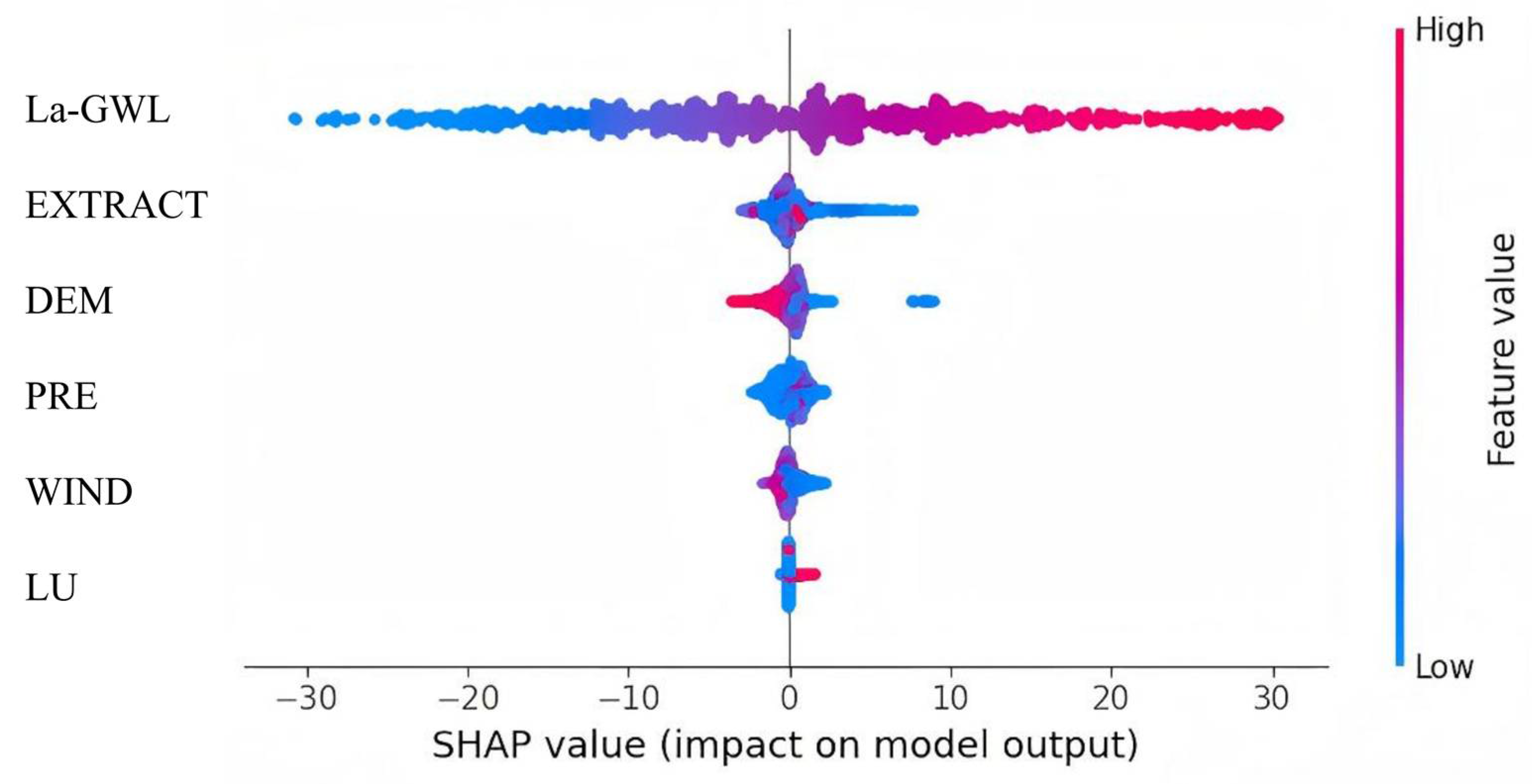
By calculating the SHAP values of feature variables and ranking their mean absolute values (Figure 16), it was found that the lagged groundwater level exhibited the highest importance in predicting current groundwater levels. This dominance is not merely a statistical artifact but is underpinned by the physical behavior of deep confined aquifers. In such systems, hydraulic responses to external disturbances are inherently delayed due to low hydraulic diffusivity, thick overburden, and limited lateral recharge pathways. These conditions cause pressure waves to propagate slowly, resulting in strong system memory.

From a theoretical perspective, confined groundwater flow is governed by the diffusion equation, which exhibits first-order temporal dependence. The current hydraulic head is directly influenced by its past states, particularly in aquifers with low transmissivity and high storage coefficients. In the study area, the third aquifer group exhibited weak connectivity with surface recharge sources. As a result, changes in groundwater levels were mainly governed by internal hydraulic gradients and historical extraction pressures, rather than short-term meteorological fluctuations. Consequently, the lagged groundwater level captured both the autocorrelated dynamics and the delayed system response, making it a physically meaningful and information-rich predictor. This interpretation is consistent with findings in traditional time series groundwater models (e.g., ARIMA), where historical levels are key inputs. The SHAP-based feature importance results thus reflect not only statistical relevance but also sound hydrogeological reasoning, reinforcing the validity of the Stacking model’s design in this study.

The mean SHAP value of extraction volume ranked second, revealing the direct control effect of artificial pumping on groundwater levels [37]. According to Theis’ theory of unsteady flow, the drawdown caused by extraction can be expressed as Equation (12):

$$s\left(r,t\right)={\displaystyle \frac{Q}{4\pi T}}W\left(u\right),$$

(12)

where $W\left(u\right)$ represents the well function, and $T$ denotes the transmissivity coefficient. The study area is in a state of overextraction, leading to a strong negative correlation between the water level and extraction volume. This is consistent with the water level decline pattern reported in global groundwater sustainability assessments for irrigated agricultural regions.

The mean SHAP values of climatic factors, such as rainfall and wind speed, were relatively low. This is because the study focused on deep groundwater levels. Rainfall infiltration experiences a long delay and cannot directly affect deep groundwater levels. Moreover, due to the relatively small temporal and spatial scales of this study, differences in land use types and ground elevation were not pronounced, and their impact on predicting deep groundwater levels was minimal [38].

4.6. Summary of Findings

In summary, the Stacking ensemble learning model demonstrated clear superiority over individual models in predicting groundwater levels. By integrating the complementary strengths of multiple base learners, it achieved higher predictive accuracy and better agreement with observed values on the overall test set. Moreover, its strong generalization performance across wells with distinct spatial distributions highlighted its robustness to hydrogeological heterogeneity. Residual and spatial error analyses further confirmed the model’s stability and adaptability under varying conditions. Moreover, SHAP-based feature interpretation demonstrated that the model consistently responded to physically meaningful variables, such as lagged groundwater levels and groundwater extraction volume. These findings collectively highlight the effectiveness of the Stacking framework in modeling groundwater systems that are complex, nonlinear, and spatially heterogeneous. They provide a robust foundation for developing reliable forecasting and management strategies for sustainable groundwater use.

5. Simulation and Prediction of the Regional Groundwater Restoration Effects by the South-to-North Water Diversion Project

5.1. Background and Methodological Framework

To quantitatively assess the hydrological restoration effects of the South-to-North Water Diversion Project (SNWDP) on regional deep groundwater systems, this study employed a comparative simulation framework based on Stacking ensemble models. Two scenarios were constructed for the period 2018–2022: one with water input from the SNWDP and one without. Kriging interpolation was used to visualize the spatiotemporal evolution of groundwater levels (GWLs), enabling an intuitive comparison of actual monitoring data with counterfactual simulation results under the non-diversion scenario.

5.2. Observed Groundwater Recovery Under the SNWDP

As shown in Figure 17, a notable regional rebound in groundwater levels was observed between 2018 and 2022. This recovery was especially pronounced in previously overexploited zones, such as the central and southern funnel areas, where the groundwater depression cones exhibited visible shrinkage. These upward trends in monitored water levels suggested a significant mitigation of aquifer depletion, plausibly attributable to the supplemental recharge provided by the SNWDP.

5.3. Simulated Counterfactual: No-SNWDP Scenario

To isolate the role of the SNWDP, the trained ensemble model was applied under a simulated condition that excluded external water diversion. The results (Figure 18) revealed a continuous decline in groundwater levels over the five-year period, particularly in the central and southern zones. Notably, the depth of the groundwater funnel expanded from −73 m in 2018 to −92 m in 2022, reflecting a 19 m drop, whereas the actual measured decline was only 7 m (to −80 m). This 12 m differential highlights the substantial influence of SNWDP inflows in curbing funnel development.

Spatially averaged groundwater levels further supported this conclusion. In June, the simulated level under the no-diversion scenario dropped from −54 m to −59 m, whereas observed levels rose by 7 m over the same period. A similar pattern was observed in December, with simulated values declining by 4 m and measured values rising by 5 m. Figure 19 illustrates this divergence, further emphasizing the positive impact of SNWDP on regional groundwater recovery.

5.4. Spatial–Temporal Differentiation of SNWDP Effects

Figure 20 presents the spatial distribution of differences between observed and simulated water levels under both scenarios. In June and December 2022, significant spatial heterogeneity was observed. The eastern region showed minimal differences (<5 m), consistent with its lower extraction density and reduced dependence on groundwater. In contrast, the southeastern and central regions exhibited the largest discrepancies, exceeding 14 m and even reaching 17 m in localized areas. These effects were more pronounced in June, coinciding with peak irrigation demand for winter wheat and maize cultivation.

This temporal asymmetry suggests that the SNWDP’s groundwater restoration function is seasonally dependent, offering the greatest hydrological relief during high-demand periods. The replacement of deep groundwater extraction with surface water effectively alleviated stress on aquifers, demonstrating the project’s crucial regulatory role in regional water resource management.

5.5. Summary of Key Findings

Collectively, these findings underscore the substantial regulatory and ecological benefits of the SNWDP. The combination of predictive modeling and counterfactual simulation provided robust quantitative evidence that the project has significantly slowed groundwater depletion, mitigated funnel expansion, and contributed to sustainable groundwater recovery in high-stress areas. The method proposed herein may serve as a transferable framework for evaluating large-scale water transfer projects in other arid or semi-arid regions facing similar groundwater crises.

6. Conclusions

This study developed a Stacking ensemble learning framework that integrates multi-source data to predict deep groundwater levels in the Cangzhou region of Hebei Province. The model was further employed to simulate the regional groundwater recovery effects under both “with water diversion” and “without water diversion” scenarios. Physically meaningful variables—such as lagged groundwater levels—were embedded into the model structure, and its performance was systematically validated in terms of generalization capability, spatial adaptability, and interpretability. The key findings are as follows.

The proposed Stacking model significantly outperformed individual machine learning models and demonstrated strong competitiveness in horizontal comparisons. On the local test dataset, the Stacking model achieved a 16.1% reduction in MAE and a 16.0% reduction in RMSE compared to the best-performing benchmark models (e.g., RF and SVR), with R² increasing to 0.88, indicating excellent fit and generalization ability. Compared with recent studies, the proposed model also showed a leading performance. For example, Jiang et al. developed an ensemble model in a plain region of northern China that yielded RMSE values ranging from 3.4 to 7.2 m and R² values from 0.71 to 0.86. In contrast, our model maintained RMSE values between 1.08 and 4.20 m, with R² reaching 0.76–0.88, suggesting stronger local adaptability and predictive stability [17].

The model structure is physically interpretable and generalizable, with good potential for integration into policy frameworks. SHAP analysis showed that lagged groundwater level and extraction volume were the most influential variables, reflecting the model’s ability to capture aquifer memory and anthropogenic impacts. Statistical tests confirmed that residuals were approximately normally distributed, with 95% of errors falling within ±10 m. The spatial pattern of residuals also aligned with variations in groundwater extraction intensity, validating the physical consistency and spatial robustness of the model.

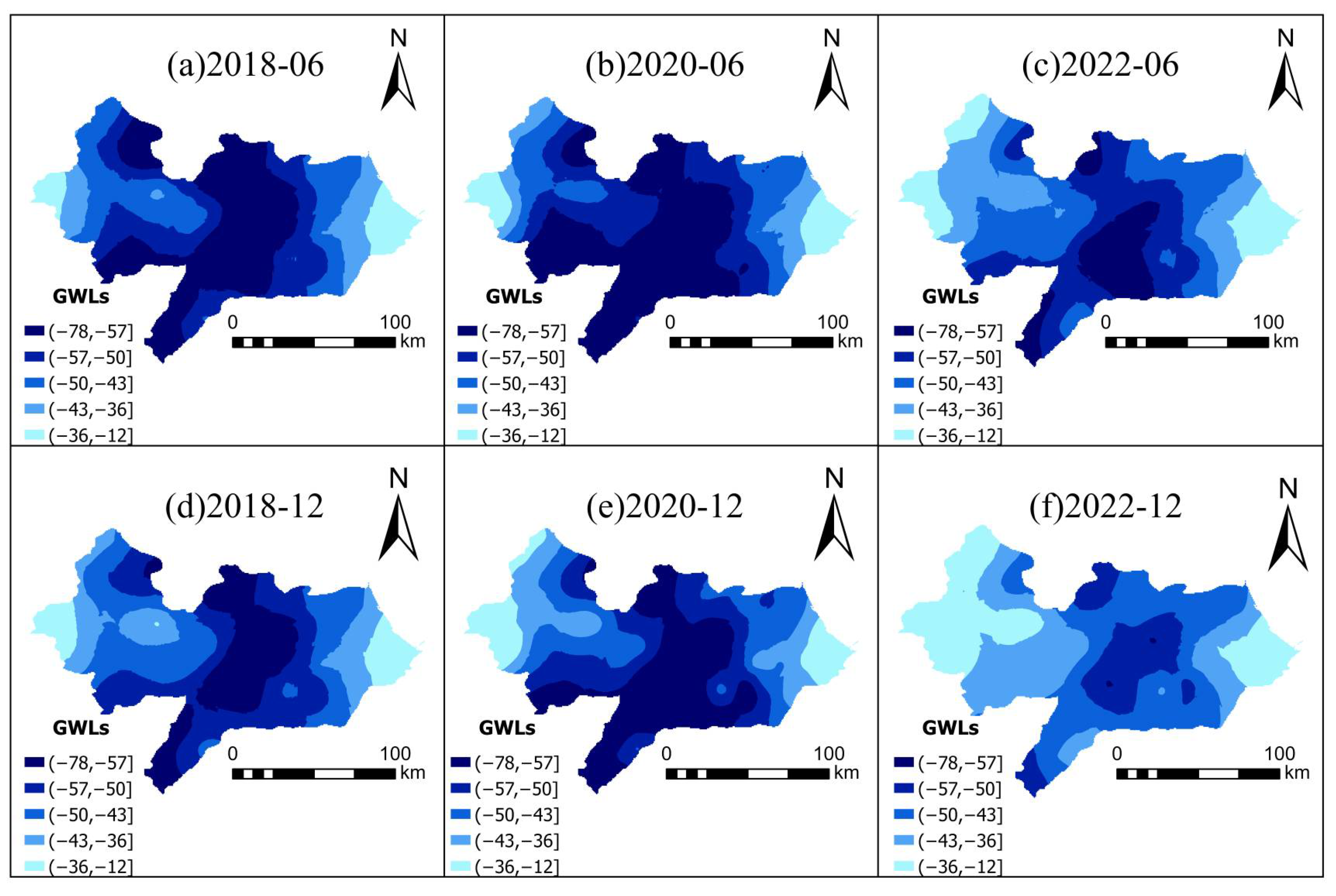
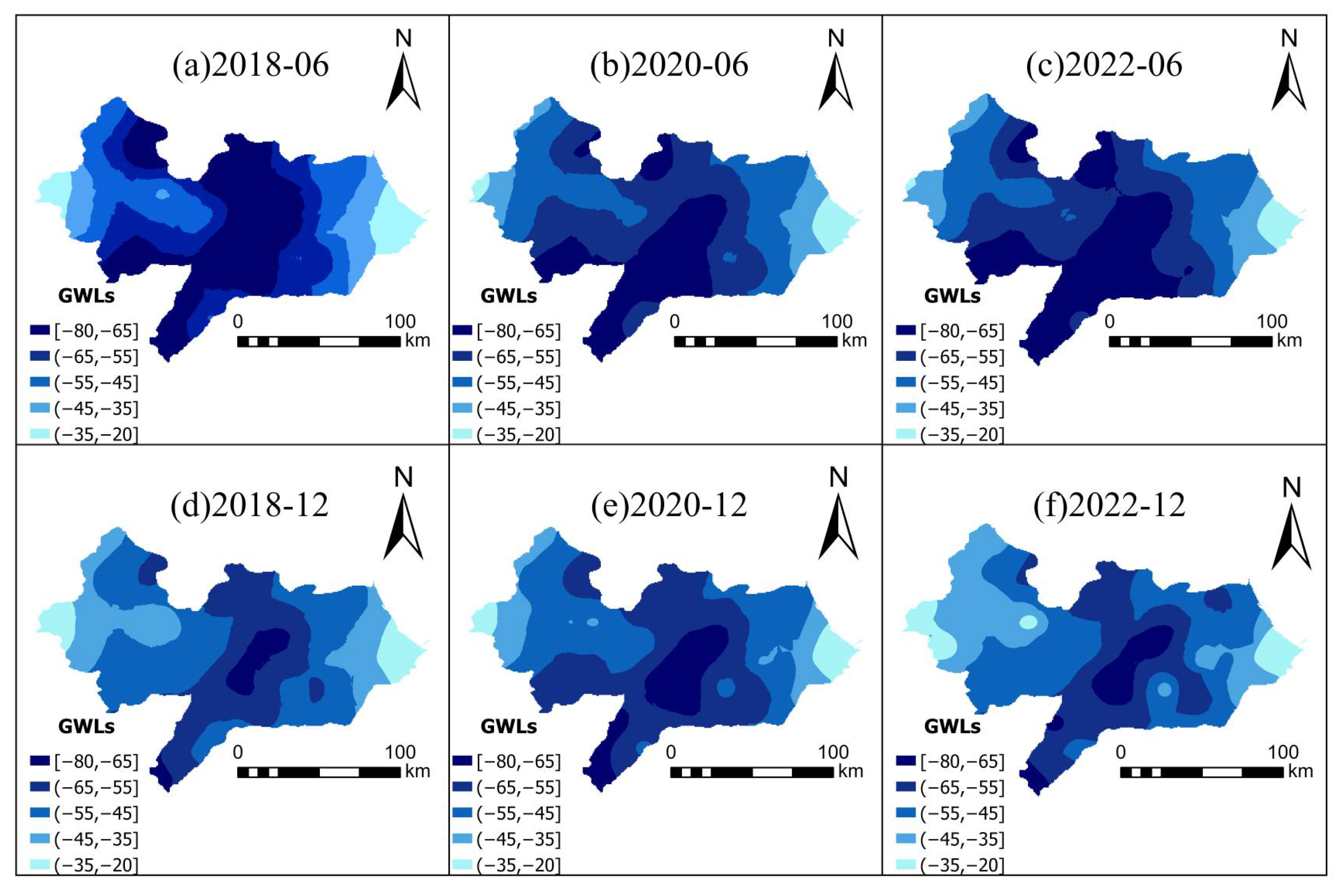
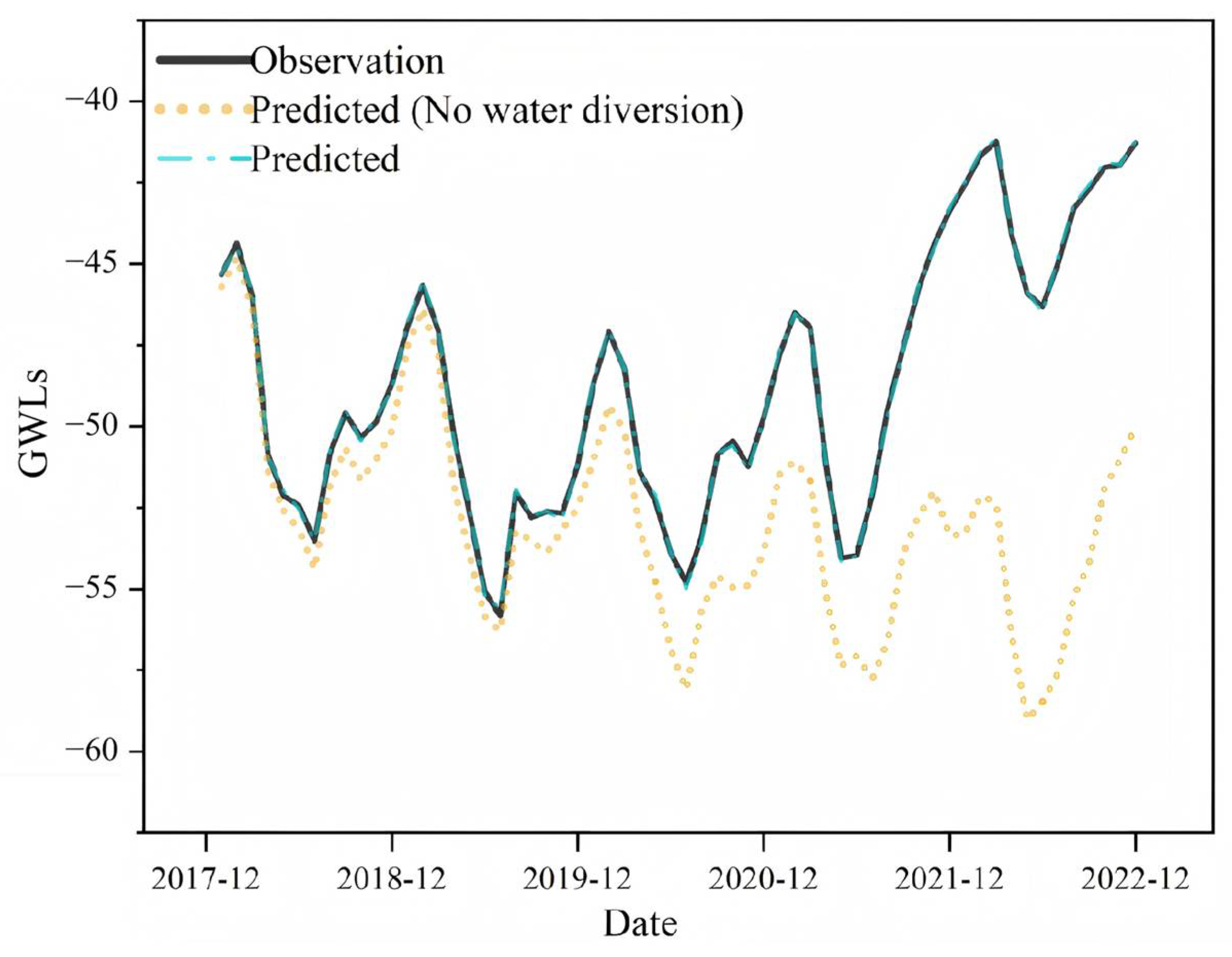
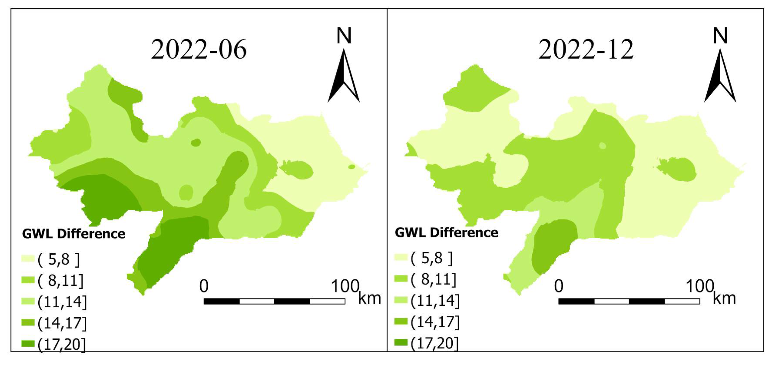
Counterfactual simulation results quantitatively confirmed the positive impact of the South-to-North Water Diversion Project (SNWDP) on groundwater recovery. Under the no-diversion scenario, the average regional groundwater level in 2022 was predicted to decline by 4–6 m, whereas observed values showed a rise of 5–7 m. In the most severely overexploited zones, the maximum difference reached 17 m, indicating that the SNWDP has played a critical ecological role in reshaping the regional water balance and mitigating groundwater overexploitation.

In terms of policy application, this study proposes two actionable water management strategies:

(1)

Establishing a dynamic groundwater warning threshold system based on model predictions, with multi-level risk zones tailored to aquifer types (e.g., “green–normal”, “yellow–excessive decline”, and “red–overexploitation alert”). Early warning mechanisms can be triggered automatically based on forecasted trends.

(2)

Optimizing the coordination between water diversion and groundwater extraction. Based on the model’s scenario simulations, a “dynamic water quota allocation” mechanism is proposed. When predicted groundwater levels fall below a predefined threshold, diversion volumes can be increased and extraction limited to restore balance. This strategy enhances the regulatory efficiency and ecological utility of large-scale diversion projects like the SNWDP.

Despite these contributions, the study has some limitations. First, the current model has not yet been validated on cross-regional or open-source datasets. Future work should benchmark the proposed model against recent approaches, such as AutoML-GWL and CatBoost-GWL. Second, the current simulation of the water diversion scenario was primarily based on extrapolated extraction data and lacks explicit representation of the groundwater–surface water interaction. We recommend integrating hybrid physical–data models (e.g., PINN and Hybrid-LSTM) in future studies to enhance long-term scenario reliability.

In conclusion, the proposed Stacking framework demonstrated strong advantages in model design, accuracy, and policy relevance. It improved the technical capacity for forecasting deep groundwater levels and offers an operational tool for adaptive groundwater regulation. The modeling approach and policy suggestions hold strong potential for replication in other water-stressed regions and can serve as a reference for sustainable groundwater management globally.

References

1. Xu, Y.; Mo, X.; Cai, Y.; Li, X. Analysis on Groundwater Table Drawdown by Land Use and the Quest for Sustainable Water Use in the Hebei Plain in China. Agric. Water Manag. 2005, 75, 38–53. [Google Scholar] [CrossRef]
2. Jianfei, F.; Lun, Z.; Zhiguo, L.; Jianying, Y. Study on the Sustainable Utilization of Groundwater Resources in Hebei Plain. Procedia Environ. Sci. 2012, 12, 1071–1076. [Google Scholar] [CrossRef]
3. Wang, J.; Jiang, Y.; Wang, H.; Huang, Q.; Deng, H. Groundwater Irrigation and Management in Northern China: Status, Trends, and Challenges. Int. J. Water Resour. Dev. 2020, 36, 670–696. [Google Scholar] [CrossRef]
4. Mukherjee, A.; Bhanja, S.N.; Wada, Y. Groundwater Depletion Causing Reduction of Baseflow Triggering Ganges River Summer Drying. Sci. Rep. 2018, 8, 12049. [Google Scholar] [CrossRef]
5. Tzampoglou, P.; Ilia, I.; Karalis, K.; Tsangaratos, P.; Zhao, X.; Chen, W. Selected Worldwide Cases of Land Subsidence Due to Groundwater Withdrawal. Water 2023, 15, 1094. [Google Scholar] [CrossRef]
6. Chen, Y.; Li, Z.; Li, W.; Deng, H.; Shen, Y. Water and Ecological Security: Dealing with Hydroclimatic Challenges at the Heart of China’s Silk Road. Environ. Earth Sci. 2016, 75, 881. [Google Scholar] [CrossRef]
7. Guo, H.; Hao, A.; Li, W.; Zang, X.; Wang, Y.; Zhu, J.; Wang, L.; Chen, Y. Land Subsidence and Its Affecting Factors in Cangzhou, North China Plain. Front. Environ. Sci. 2022, 10, 1053362. [Google Scholar] [CrossRef]
8. Zeydalinejad, N. Artificial Neural Networks Vis-à-Vis MODFLOW in the Simulation of Groundwater: A Review. Model. Earth Syst. Environ. 2022, 8, 2911–2932. [Google Scholar] [CrossRef]
9. Boo, K.B.W.; El-Shafie, A.; Othman, F.; Khan, M.M.H.; Birima, A.H.; Ahmed, A.N. Groundwater Level Forecasting with Machine Learning Models: A Review. Water Res. 2024, 252, 121249. [Google Scholar] [CrossRef]
10. Singh, A.; Patel, S.; Bhadani, V.; Kumar, V.; Gaurav, K. AutoML-GWL: Automated Machine Learning Model for the Prediction of Groundwater Level. Eng. Appl. Artif. Intell. 2024, 127, 107405. [Google Scholar] [CrossRef]
11. LaBianca, A.; Koch, J.; Jensen, K.H.; Sonnenborg, T.O.; Kidmose, J. Machine Learning for Predicting Shallow Groundwater Levels in Urban Areas. J. Hydrol. 2024, 632, 130902. [Google Scholar] [CrossRef]
12. Azizi, E.; Yosefvand, F.; Yaghoubi, B.; Izadbakhsh, M.A.; Shabanlou, S. Prediction of Groundwater Level Using GMDH Artificial Neural Network Based on Climate Change Scenarios. Appl. Water Sci. 2024, 14, 77. [Google Scholar] [CrossRef]
13. Bai, Z.; Liu, Q.; Liu, Y. Groundwater Potential Mapping in Hubei Region of China Using Machine Learning, Ensemble Learning, Deep Learning and AutoML Methods. Nat. Resour. Res. 2022, 31, 2549–2569. [Google Scholar] [CrossRef]
14. Shen, C. A Transdisciplinary Review of Deep Learning Research and Its Relevance for Water Resources Scientists. Water Resour. Res. 2018, 54, 8558–8593. [Google Scholar] [CrossRef]
15. Cao, W.; Zhang, Z.; Fu, Y.; Zhao, L.; Ren, Y.; Nan, T.; Guo, H. Prediction of Arsenic and Fluoride in Groundwater of the North China Plain Using Enhanced Stacking Ensemble Learning. Water Res. 2024, 259, 121848. [Google Scholar] [CrossRef]
16. Eldin Elzain, H.; Abdalla, O.; Al-Maktoumi, A.; Kacimov, A.; Eltayeb, M. A Novel Approach to Forecast Water Table Rise in Arid Regions Using Stacked Ensemble Machine Learning and Deep Artificial Intelligence Models. J. Hydrol. 2024, 640, 131668. [Google Scholar] [CrossRef]
17. Jiang, Z.; Yang, S.; Liu, Z.; Xu, Y.; Shen, T.; Qi, S.; Pang, Q.; Xu, J.; Liu, F.; Xu, T. Can Ensemble Machine Learning Be Used to Predict the Groundwater Level Dynamics of Farmland under Future Climate: A 10-Year Study on Huaibei Plain. Environ. Sci. Pollut. Res. 2022, 29, 44653–44667. [Google Scholar] [CrossRef]
18. Du, Z.; Ge, L.; Ng, A.H.-M.; Lian, X.; Zhu, Q.; Horgan, F.G.; Zhang, Q. Analysis of the Impact of the South-to-North Water Diversion Project on Water Balance and Land Subsidence in Beijing, China between 2007 and 2020. J. Hydrol. 2021, 603, 126990. [Google Scholar] [CrossRef]
19. Huang, Y.; Yang, J.; Yu, X.; Wang, S.; Xie, X.; Li, J.; Wang, Y. Hydrogeochemical Analysis and Paleo-Hydrogeological Modeling of Shallow Groundwater Salinization Processes in North China Plain. J. Hydrol. 2025, 651, 132616. [Google Scholar] [CrossRef]
20. Benesty, J.; Chen, J.; Huang, Y. Microphone Array Signal Processing; Springer: Berlin/Heidelberg, Germany, 2019; ISBN 9783540786115. [Google Scholar]
21. Kraskov, A.; Stögbauer, H.; Grassberger, P. Estimating Mutual Information. Phys. Rev. E 2004, 69, 066138. [Google Scholar] [CrossRef] [PubMed]
22. Wolpert, D.H. Stacked Generalization. Neural Netw. 1992, 5, 241–259. [Google Scholar] [CrossRef]
23. Huang, Y.; Feng, X.; Li, B.; Xiang, Y.; Wang, H.; Qin, B.; Liu, T. Ensemble Learning for Heterogeneous Large Language Models with Deep Parallel Collaboration. 2024. Available online: https://openreview.net/forum?id=7arAADUK6D&referrer=%5Bthe%20profile%20of%20Xiaocheng%20Feng%5D (accessed on 21 May 2025).
24. Mienye, I.D.; Sun, Y. A Survey of Ensemble Learning: Concepts, Algorithms, Applications, and Prospects. IEEE Access 2022, 10, 99129–99149. [Google Scholar] [CrossRef]
25. Chenjia, Z.; Xu, T.; Zhang, Y.; Ma, D. Deep Learning Models for Groundwater Level Prediction Based on Delay Penalty. Water Supply 2024, 24, 555–567. [Google Scholar] [CrossRef]
26. Yadav, B.; Gupta, P.K.; Patidar, N.; Himanshu, S.K. Ensemble Modelling Framework for Groundwater Level Prediction in Urban Areas of India. Sci. Total Environ. 2020, 712, 135539. [Google Scholar] [CrossRef]
27. Patra, S.; Sahoo, S.; Mishra, P.; Mahapatra, S.C. Impacts of Urbanization on Land Use/Cover Changes and Its Probable Implications on Local Climate and Groundwater Level. J. Urban Manag. 2018, 7, 70–84. [Google Scholar] [CrossRef]
28. China Meteorological Administration. Historical Climate Element Data Query for Cangzhou Area. China Meteorological Data Net. Available online: https://data.cma.cn/data/detail/dataCode/A.0019.0001.S001.html (accessed on 25 January 2025).
29. Chinese Academy of Sciences Resource and Environment Sciences Data Center. China Land Use Remote Sensing Monitoring Dataset. 2023. Available online: https://www.resdc.cn/Datalist1.aspx?FieldTyepID=5,2 (accessed on 25 January 2025).
30. Cover, T.; Hart, P. Nearest Neighbor Pattern Classification. IEEE Trans. Inf. Theory 1967, 13, 21–27. [Google Scholar] [CrossRef]
31. Rumelhart, D.E.; Hinton, G.E.; Williams, R.J. Learning Representations by Back-Propagating Errors. Nature 1986, 323, 533–536. [Google Scholar] [CrossRef]
32. Lecun, Y.; Bottou, L.; Bengio, Y.; Haffner, P. Gradient-Based Learning Applied to Document Recognition. Proc. IEEE 1998, 86, 2278–2324. [Google Scholar] [CrossRef]
33. Breiman, L. Random Forest. Mach. Learn. 2001, 45, 5–32. [Google Scholar] [CrossRef]
34. Chen, T.; Guestrin, C. XGBoost. In Proceedings of the 22nd ACM SIGKDD International Conference on Knowledge Discovery and Data Mining, San Francisco, CA, USA, 13–17 August 2016; ACM: New York, NY, USA, 2016; pp. 785–794. [Google Scholar]
35. Vapnik, V.N. The Nature of Statistical Learning Theory; Springer: New York, NY, USA, 2000; ISBN 978-1-4419-3160-3. [Google Scholar]
36. Van den Broeck, G.; Lykov, A.; Schleich, M.; Suciu, D. On the Tractability of SHAP Explanations. J. Artif. Intell. Res. 2022, 74, 851–886. [Google Scholar] [CrossRef]
37. Ataie Ashtiani, B.; Simmons, C.T.; Farhadi, L.; Zhang, S. Groundwater Sustainability Assessment and the Research-Practice Nexus. J. Hydrol. 2024, 644, 132166. [Google Scholar] [CrossRef]
38. Wu, Y.; Yin, X.; Zhou, G.; Bruijnzeel, L.A.; Dai, A.; Wang, F.; Gentine, P.; Zhang, G.; Song, Y.; Zhou, D. Rising Rainfall Intensity Induces Spatially Divergent Hydrological Changes within a Large River Basin. Nat. Commun. 2024, 15, 823. [Google Scholar] [CrossRef] [PubMed]
Figure 1. Study area.
Sustainability 17 06120 g001
Figure 2. Geological profile of the Cangzhou region.
Sustainability 17 06120 g002
Figure 3. Pearson–MI-based feature selection framework.
Sustainability 17 06120 g003
Figure 4. Stacking ensemble learning process.
Sustainability 17 06120 g004
Figure 5. K-fold cross-validation.
Sustainability 17 06120 g005
Figure 6. Preprocessing flowchart.
Sustainability 17 06120 g006
Figure 7. Model framework diagram.
Sustainability 17 06120 g007
Figure 8. Architecture of the weighted average meta-learner.
Sustainability 17 06120 g008
Figure 9. Feature correlation matrix (a) and mutual information scores (b).
Sustainability 17 06120 g009
Figure 10. Comparison of observed and predicted values on the test set for various models. (a) SVR; (b) XG-Boost; (c) MLP; (d) CNN; (e) RF; (f) KNN; (g) Stacking.
Sustainability 17 06120 g010
Figure 11. Comparison of model evaluation metrics.
Sustainability 17 06120 g011
Figure 12. Comparison of model performance. (a) Well 1; (b) Well 2; (c) Well 3; (d) Well 4.
Sustainability 17 06120 g012
Figure 13. Prediction results of representative observation wells. (a) Well 1; (b) Well 2; (c) Well 3; (d) Well 4.
Sustainability 17 06120 g013
Figure 14. Histogram of error distribution.
Sustainability 17 06120 g014
Figure 15. Spatial residual map of the test set (2022).
Sustainability 17 06120 g015
Figure 16. SHAP values of feature variables.
Sustainability 17 06120 g016
Figure 17. Observed values of actual water levels.
Sustainability 17 06120 g017
Figure 18. Predicted values under the condition without the South-to-North Water Diversion Project.
Sustainability 17 06120 g018
Figure 19. Comparison between observed average groundwater level values and predicted water level values under the condition without the South-to-North Water Diversion Project.
Sustainability 17 06120 g019
Figure 20. The difference between the measured water level and simulated water level under the scenario without water diversion from the South-to-North Water Diversion Project.
Sustainability 17 06120 g020