Threshold Soil Moisture Levels Influence Soil CO₂ Emissions: A Machine Learning Approach to Predict Short-Term Soil CO₂ Emissions from Climate-Smart Fields

Abstract

Machine learning (ML) models are widely used to analyze the spatiotemporal impacts of agricultural practices on environmental sustainability, including the contribution to global greenhouse gas (GHG) emissions. Management practices, such as organic amendment applications, are critical pillars of Climate-smart agriculture (CSA) strategies that mitigate GHG emissions while maintaining adequate crop yields. This study investigated the critical threshold of soil moisture level associated with soil CO₂ emissions from organically amended plots using the classification and regression tree (CART) algorithm. Also, the study predicted the short-term soil CO₂ emissions from organically amended systems using soil moisture and weather variables (i.e., air temperature, relative humidity, and solar radiation) using multilinear regression (MLR) and generalized additive models (GAMs). The different organic amendments considered in this study are biochar (2268 and 4536 kg ha⁻¹) and chicken and dairy manure (0, 224, and 448 kg N/ha) under a sweet corn crop in the greater Houston area, Texas. The results of the CART analysis indicated a direct link between soil moisture level and the magnitude of CO₂ flux emission from the amended plots. A threshold of 0.103 m³m⁻³ was calculated for treatment amended by biochar level I (2268 kg ha⁻¹) and chicken manure at the N recommended rate (CXBX), indicating that if the soil moisture is less than the 0.103 m³m⁻³ threshold, then the median soil CO₂ emission is 142 kg ha⁻¹ d⁻¹. Furthermore, applying biochar at a rate of 4536 kg ha⁻¹ reduced the soil CO₂ emissions by 14.5% compared to the control plots. Additionally, the results demonstrate that GAMs outperformed MLR, exhibiting the highest performance under the combined effect of chicken and biochar. We conclude that quantifying soil moisture thresholds will provide valuable information for the sustainable mitigation of soil CO₂ emissions.

1. Introduction

Global maize yield has decreased by 3.8% because of climate extremes, and research findings indicate a steep decrease in crop productivity when temperatures exceed critical physiological thresholds [1,2,3,4]. The impact of extreme climate events can be long-lasting and disrupt the agricultural commodity market. Also, agriculture is a principal contributor to climate change-induced global warming, contributing 10–12% of global anthropogenic emissions [5,6]. A major source of greenhouse gas (GHG) emissions in agriculture stems from how cropland soils are managed, particularly through practices such as intensive tillage and manure application. Also, according to the Food and Agriculture Organization, global food production needs to increase by 70% to feed two billion more people by 2050. Therefore, we need to improve soil management practices to meet this escalating food demand. Thus, adequate conservation and sustainable practices are necessary to minimize GHG emissions while improving crop yields.

Nitrous oxide (N₂O), carbon dioxide (CO₂), and methane (CH₄) are the main GHGs emitted from agricultural fields, where methane and nitrous oxide account for about 80% of emissions, and carbon dioxide contributes the remaining 20% [7]. According to the US Environmental Protection Agency (EPA), total GHG emissions from the US agricultural sector in 2019 amounted to 10%, and the major contributor was the crop cultivation sector (55%). Therefore, there is an urgent need to adopt a management solution that will reduce GHG contributions from agricultural systems. Climate-smart agriculture (CSA) is a strategy to address the challenges of climate change and food security through sustainable agricultural production and reducing GHG emissions [8]. Also, the Intergovernmental Panel on Climate Change (IPCC) projections [2] highlight the vulnerability of agricultural systems and the increased threat to global food security in the absence of CSA measures. The use of organic inputs is often recommended to help farmers achieve CSA goals. These practices also improve soil health, fertility, and water conservation.

Sweet corn (Zea mays L. subsp. Mays) is grown on about 500,000 farms across the United States annually and is worth about USD 775 million [9]. Soils may not meet the nitrogen (N) requirement of sweet corn; therefore, growers tend to apply soil amendments (inorganic or organic) rich in N, P (phosphorus), and K (potassium) [10,11]. In general, as an effort toward CSA and environmentally friendly farming, many growers are shifting from conventional inorganic fertilizers to more sustainable organic alternatives [12]. Also, organic soil amendments contribute to long-term sustainability by enhancing soil health through improved physical, chemical, and biological properties, including soil fertility, nutrient availability, soil aeration, and water-holding capacity [13]. However, to boost yield, growers often apply amendments at rates higher than the crop requires [12]. Thus, excessive application not only undermines input-use efficiency but may also elevate GHG emissions, even within CSA systems [14].

In general, agricultural fields can function as carbon sources and sinks depending on various factors, such as management practices; thus, it is crucial to evaluate the soil CO₂ flux to understand whether the movement of carbon is into or out of the system [10,15]. Also, weather variables could significantly impact CO₂ emissions from the crop fields [16]. Therefore, identifying the major factors that control CO₂ fluxes from the agricultural field is crucial for minimizing the agricultural sector’s contribution to global warming. Many modeling approaches have been developed to simulate soil CO₂ emissions from agricultural lands. Among them, process-based biogeochemical simulators such as CENTURY, RothC, DNDC, and DayCent are widely used to quantify emissions from farm fields [16]. In general, these models translate field-scale drivers such as temperature, moisture, texture, and management into mechanistic estimates of carbon turnover and respiration, which can be upscaled to a regional scale. For example, the DayCent model is capable of quantifying finer temporal scales and layered soil-level CO₂ emissions from various cropping systems [5,14]. The DNDC (DeNitrification–DeComposition) model couples C and N biogeochemistry under aerobic and anaerobic conditions, simulating crop growth, hydrology, and multi-gas fluxes [14]. These models enable researchers to quantify management impacts on soil CO₂ emissions and develop mitigation strategies. Machine learning (ML) can be crucial in quantifying GHG emissions from agricultural fields by identifying the key determining factors, such as soil management practices and weather variables, that influence these emissions [17,18].

Soil moisture plays a critical role in organic matter decomposition and in supporting sustainable soil microbial activity. Adequate soil water content is required for decomposition and succeeding CO₂ emissions [16,19,20]. However, extremely dry or waterlogged conditions can disrupt the soil’s ecological balance, limiting microbial activity and potentially reducing CO₂ emissions. The combination of poor drainage and excessive soil water may enhance the growth of anaerobic microbes, which can increase soil CO₂ production through anaerobic respiration [21,22]. The influence of soil moisture on CO₂ emissions is shaped by multiple sustainability-related factors, including organic amendment types and rates, irrigation management, and the unique environmental conditions of each site. Therefore, identifying optimal soil moisture conditions to manage soil CO₂ emissions is critical in climate change research. Despite research efforts to examine the relationship between CO₂ emissions and soil moisture levels, improved understanding and quantification of moisture thresholds that can link the soil moisture level to CO₂ fluxes helps farmers and ranchers to take timely actions to mitigate emissions and improve carbon sequestration. To address this limitation, we developed a ‘threshold’ for soil moisture that directly links the soil moisture level with CO₂ emissions. The specific goals of our research are (i) to quantify the amount of soil CO₂ emissions from different amendment types (biochar, chicken, and dairy manure) and application rates in sweet corn plots, (ii) to identify the critical threshold of soil moisture that is directly linked to CO₂ emissions from treatments, (iii) to predict and compare the soil CO₂ emissions by applying multilinear regression and generalized additive models using soil moisture and weather variables. We applied the classification and regression tree (CART) concept to identify soil moisture thresholds that could be used to support sustainable soil CO₂ emission mitigation strategies.

2. Materials and Methods

The experimental and machine learning framework developed for quantifying the impact of soil moisture and temperature on soil CO₂ emissions from this study is depicted in Figure 1. The following sections provide a succinct description of individual components incorporated into the study.

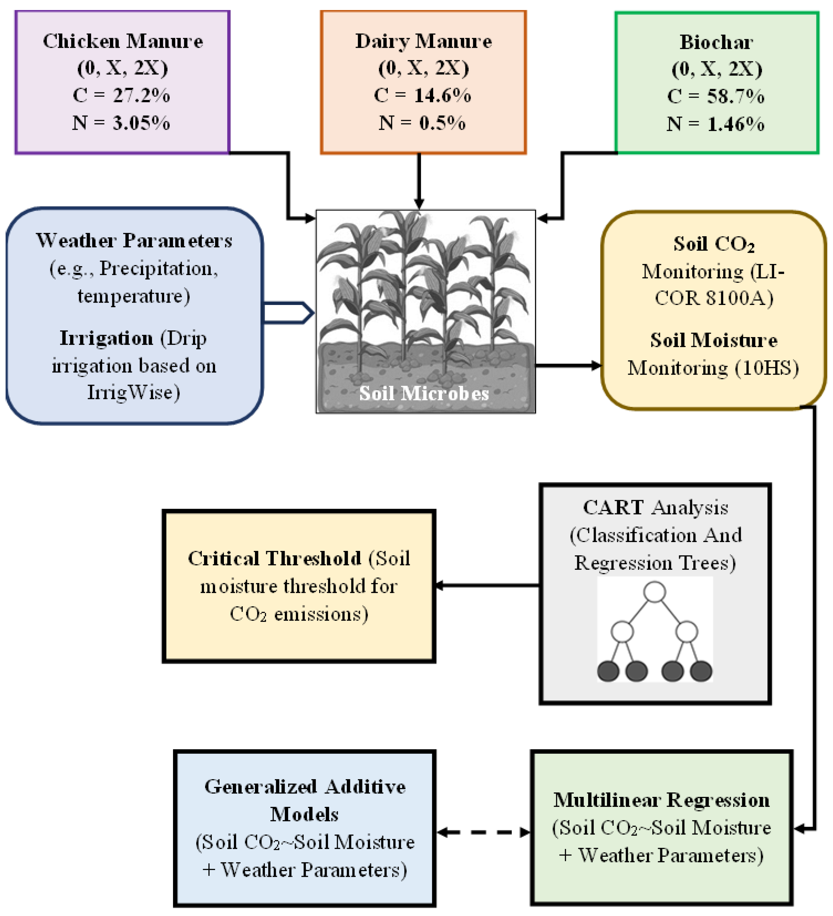
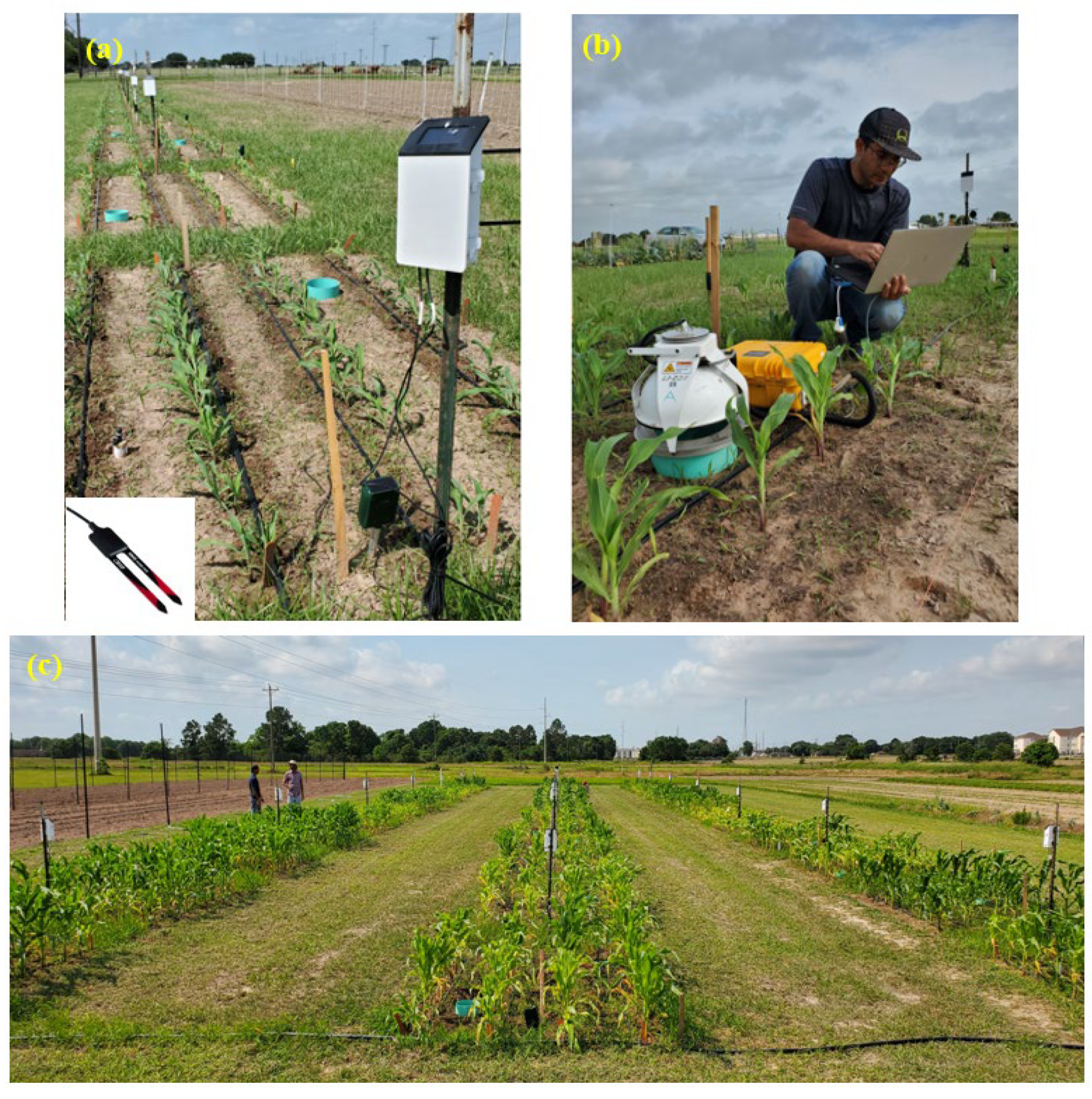
2.1. Study Site and Experimental Design

The experimental work was conducted at the Prairie View A&M University Research Farm located in the vicinity of Houston, Texas (Figure 2). The annual rainfall at the study site is 1118 mm, with 60% falling between June and October. The study area exhibits a humid subtropical climate and experiences a yearly average temperature of 17.2 °C. Summers are hot, whereas winters are comparatively colder. The hottest month is July, with an average air temperature of 35 °C, and the coldest month is January, with an average air temperature of 3 °C. Weather variables, including precipitation, temperature, wind speed, relative humidity, and solar radiation, were monitored at a 15 min interval via a WatchDog 2000 series Portable weather station (Figure 3, Spectrum Technologies, Inc., Aurora, IL, USA) installed at the experimental site. A summary of weather variables during the experimental season is illustrated in Figure 4. The soil at the site is classified as a Wockley fine sandy loam (fine-loamy, siliceous, semiactive, hyperthermic Plinthaquic Paleudalfs) [23].

The experimental design was a factorial Randomized Complete Block Design (RCBD) with three replications (Figure 2). Two organic amendments used in the experiment were chicken and dairy manure with an application rate of 0, 224, and 448 kg N ha⁻¹, hereafter referred to as control, recommended, and double recommended rates, respectively. Similarly, as a sub-factor, biochar was applied at a rate of 2268 and 4536 kg ha⁻¹, hereafter referred to as Level I and II, respectively. Each treatment was replicated three times. The biochar used in this study was obtained from coconut husk and sourced from the Andersons BioChar DG Organic Soil Amendment. Figure 2 illustrates the layout of the experimental design. X indicates the recommended manure/Level I biochar rate. Similarly, 2X indicates the double recommended manure/Level II biochar rates. Sweet corn was grown in the plots using a drip irrigation system to ensure consistent and efficient water delivery throughout the growing period. The soil chemical properties, including nutrient concentration, pH, and electrical conductivity (EC), were determined in the laboratory and have been previously discussed in an earlier study [11]. The total carbon content of the biochar was relatively higher than that of chicken and dairy manure. The highest pH value was observed for dairy manure (8.4), and biochar registered the lowest pH (5.67). Before planting, organic amendments were broadcast, mixed, and incorporated into the top 15 cm. The sweet corn was sown on 15 April 2022. Slow-release nitrogen fertilizers supply plants with adequate nutrients in climate-smart practices. However, many growers tend to apply more than the recommended rate of organic manure. This study used three rates of organic manure (i.e., zero or no fertilizer, recommended rate, and double recommended rate) and two levels of biochar application (i.e., Levels I and II).

2.2. Irrigation Management

The plots were irrigated using a drip irrigation system. The irrigation events were scheduled based on IrrigWise, a web-based irrigation scheduling tool, using near-real-time site-specific rainfall, reference evapotranspiration, soil water content, and plant growth stage [24]. IrrigWise uses data from several databases, including the USDA-NRCS’ Soil Survey Geographic Database (Soil Survey Staff, n.d.), daily rainfall, and evapotranspiration from multiple weather networks across Texas. Eighteen irrigation events were scheduled during the growing season to meet the crop water demand.

2.3. Soil Moisture Monitoring

Soil moisture sensors were installed in all 39 plots to monitor sub-daily soil water content at 0–10 cm (within the root zone) and 30–40 cm (below the root zone) below the soil surface (Figure 3a). The sensor 10HS (METER Group Inc., Pullman, WA, USA), which measures volumetric water content using the Frequency Domain Reflectometry technique, was used for measuring the plot soil water content at a 15 min interval [25,26]. It uses a 70 MHz frequency to minimize the textural, salinity, and temperature effects in most agricultural environments. The data monitored by these sensors were logged to a data logger, which was downloaded to the computer via a USB cable. Readings are provided directly in volumetric water content (m³m⁻³) based on the manufacturer’s default calibration equation.

2.4. Soil CO₂ Flux Measurement

During the growing season, soil CO₂ emissions were measured using an LI-8100A (LI-COR Biosciences, Lincoln, NE, Figure 3b) survey system. The soil CO₂ emissions were measured from the same location of the plot using a collar (20 cm survey chamber) installed at each plot. The LI-8100A system includes a data logger, survey chamber, and soil collar. LI-COR Biosciences’ proprietary Soil-Flux-Pro (version 5.2) software was used to operate the system and analyze the collected soil CO₂ emission data.

For the experimental period, soil CO₂ emissions were measured twice a week (Monday and Thursday). The measurements were performed between 9:00 and 11:00 a.m., which is considered the optimal sampling time to represent the daily average soil CO₂ emissions [10].

2.5. Statistical Analysis

The effects of amendment types and rates on soil CO₂ emissions were investigated using Analysis of Variance (ANOVA), determining whether the treatments had any significant effects. Tukey’s mean separation was performed to separate the effects of different treatments on soil CO₂ emissions at a 5 percent significance level. Statistical analyses were conducted using the Statistix 10 software package (Analytical Software 2015, Tallahassee, FL, USA).

2.6. Trend Analysis

The trends in soil CO₂ emissions were analyzed using the Mann–Kendall test [27] and linear regression. The Mann–Kendall test is a non-parametric method used for data series without specific distributions. Simple linear regression assumes a linear relationship between the variables and relies on the normality of the residuals. In contrast, the Mann–Kendall test does not rely on the distribution of data; it is robust to the presence of outliers. In terms of slope, linear regression quantifies the average rate of change in the CO₂ emissions with respect to time. The Mann–Kendall test statistic is denoted as tau (τ), representing the sum of the signs of the differences between pairs of data points. I.e., τ represents the proportion of soil CO₂ emissions up and down movement against time. A positive τ value indicates an increasing trend, while a negative value indicates a decreasing trend. τ is calculated as follows.

$$\mathsf{\tau }={\sum }_{i=1}^{n-1}{\sum }_{j=i+1}^{n}sgn(x_j-x_i)$$

(1)

where n is the number of observed CO₂ emission data, $x_j-x_i$ are data values at different time points, and sgn is the sign of data values at different points.

2.7. Classification and Regression Tree

The Classification and Regression Tree (CART) models were developed to identify the soil moisture threshold associated with the soil CO₂ emissions from all plots. CART is a resilient machine learning algorithm in which the datasets are segregated into subsets with homogeneous values of a dependent variable [28]. This procedure entails creating a tree-like framework comprising a root node, branches, internal nodes, and leaf nodes [29]. As a result, CART aptly captures the incremental decision-making process of intricate systems by organizing the predictor space into numerous straightforward regions according to the output variable [29]. In addition, the CART outcomes are better than standard regression models, specifically during the presence of non-linear relationships and interactions. CART produces easy-to-understand models with any combination of continuous/discrete variables. In CART, splitting rules that divide the variable input spaces (soil moisture) into various classes are characterized as a tree. In this tree structure, the nodes generate a threshold for each soil moisture class, which controls the soil CO₂ emissions.

Here, we developed CART models to identify each treatment’s soil moisture threshold associated with soil CO₂ emission. The process for constructing decision trees to determine the threshold of soil moisture sensors involves the following steps:

(1)

Selection of the response variable (soil CO₂ emission) and the input variable (soil moisture) for each organically amended plot.

(2)

Partitioning the input variable space X1, X2,…, Xp into J discrete and non-intersecting regions, denoted as R1, R2,…, RJ.

(3)

For each variable falling within region Rj, the tree generates the same prediction, which corresponds to the mean of the system response values in that region [29,30].

The objective of segmenting the predictor space into distinct regions is to minimize the residual sum of squares (RSS), calculated as follows:

$$RS{S}_{Min}={\sum }_{j=1}^J{\sum }_{i\in R_j}{\left(y_i-{\hat{y}}_{R_j}\right)}^2$$

(2)

where ${\hat{y}}_{R_j}$ is the mean response of the soil CO₂ emissions within the jth region. The decision tree algorithm employs recursive binary splitting, following a top-down approach. This involves effectively dividing the predictor space into two new branches further down the tree through successive splits. To perform the recursive binary splitting, we first selected the predictor Xj and the threshold ‘s’ (Equations (2) and (3)) so that splitting the predictor space can lead to the maximum reduction in RSS.

$$R_1(j,s)=\left\{X|X_j<s\right\}$$

(3)

$$R_2\left(j,s\right)=\left\{X|X_j\ge s\right\}$$

(4)

The tree output divides data into a series of nodes, and each node represents the ranges of soil CO₂ emissions in the form of a boxplot. The ultimate tree furnishes thresholds linked to soil moisture and significance values (p-value). For the development of decision trees, we utilized the Party package in RStudio (version 2024.04.0) [31]. The analysis was conducted individually for each organic amendment type and rate.

2.8. Multilinear Regression

Multiple Linear Regression (MLR) quantifies the linear relationship between the explanatory (independent) and response (dependent) variables. Here, we used the air temperature and soil moisture to predict the rate of soil CO₂ emissions from each organic amendment type and rate plot. The generic form of MLR is as follows,

$$Y_i={\beta }_0+{\beta }_1{X}_1+{\beta }_2{X}_2+\dots +{\beta }_p{X}_p+ϵ$$

(5)

where Xj represents the jth predictor and βj quantifies the association between that variable and the response. We interpret βj as the average effect on Y of a one-unit increase in Xj, holding all other predictors fixed. In this study, plot-specific MLR is developed for all of the different treatment types and rates.

2.9. Generalized Additive Models (GAMs)

GAMs provide a general framework for extending a linear regression model by allowing non-linear functions to each variable while maintaining additivity. Generalized additive models (GAMs), like ordinary linear regression, can handle both qualitative and quantitative responses [29]. Instead of assuming a strictly linear effect β_jX_ij for each predictor, GAMs replace it with a smooth, non-linear function fj (X_ij), allowing each covariate to relate to the response in a flexible, data-driven way.

$$Y_i={\beta }_0+{\sum }_{j=1}^p{f}_j\left(X_{ij}\right)+{ϵ}_i$$

(6)

$$Y_i={\beta }_0+f_1\left(X_{i1}\right)+f_2\left(X_{i2}\right)+\cdots +f_p\left(X_{ip}\right)+{ϵ}_i$$

(7)

A GAM is also called an additive model because it separately calculates fj for each X_j and adds their contributions to the model. GAM also considers the degrees of freedom (df), and part of the model-fitting process is choosing the appropriate degree of smoothness, reflecting the degree of non-linearity of a curve. A df equal to 1 is equivalent to a linear relationship, 1 < df ≤ 2 is considered a weak non-linear relationship, and df > 2 implies a highly non-linear relationship.

2.10. Model Performance Evaluation

The experimental data collected in this study are from a single season of a sweet corn crop. The total number of soil CO₂ measurement events was 25 (i.e., the total number of data points, 3 replicates × 25 = 75). The models are generated for all of the collected data. Model performance was evaluated using Pearson correlation (r), root mean square error (RMSE), and percent bias (PBIAS). In the case of r, relationship values range from −1 to +1 depending on the value sign, and there is no correlation between the two variables when this value is equal to 0. For example, the Pearson correlation between soil moisture and soil CO₂ is calculated as follows:

$$r={\displaystyle \frac{{\sum }_{k=1}^n({CO}_2-{CO}_{\mathrm{2m}})(SM-{SM}_m)}{\sqrt{{\sum }_{k=1}^n{({CO}_2-{CO}_{2m})}^2{\sum }_{k=1}^n{(SM-{SM}_m)}^2}}}$$

(8)

where CO_2m and SMm represent the soil CO₂ emissions and soil moisture, respectively, and n is the number of data points.

RMSE measures how far predictions fall from measured true values using Euclidean distance. The equation for calculating the RMSE is as follows:

$$RMSE=\sqrt{{\displaystyle \frac{{\sum }_{i=1}^n{(x_i-y_i)}^2}{N}}}$$

(9)

where n is the total number of data points, x_i is the actual observations of soil CO₂ emissions, and y_i is the predicted soil CO₂ emissions.

Percent bias (PBIAS) measures the average tendency of the predicted soil CO₂ emissions to be larger or smaller than the measured values.

$$PBIAS={\displaystyle \frac{{\sum }_{i=1}^n(x_i-y_i)}{{\sum }_{i=1}^n\left(x_i\right)}}$$

(10)

where x_i is the actual observation of soil CO₂ emissions, and y_i is the predicted soil CO₂ emissions.

3. Results and Discussion

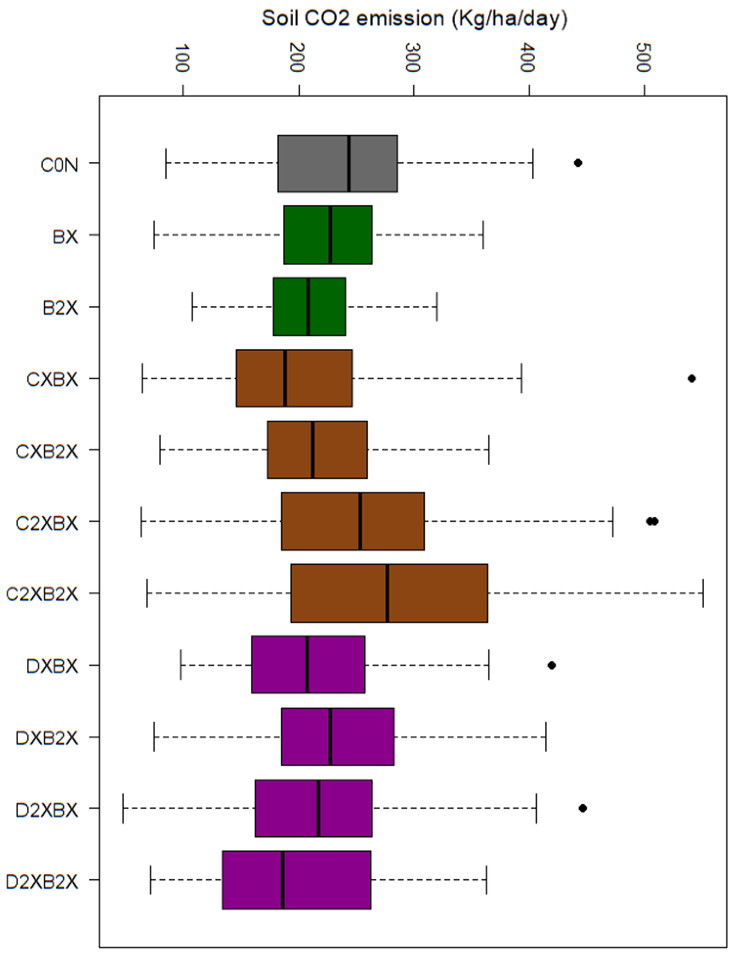
3.1. Impact of Soil Amendments on CO₂ Emissions

Applying different organic amendments at different rates resulted in varying soil CO₂ emissions. Analysis of variance reveals a highly significant correlation (p-value < 0.05) between the type and rate of manure and soil CO₂ emissions (

Table 1. ANOVA results showing the significance of organic amendment on the soil CO₂ emissions.

SOV	D.F.	Significance
Type	1	**
Rate	2	**
Biochar	1	N.S.
Type × Rate	2	**
Type × Biochar	1	*
Rate × Biochar	2	**
Type × Rate × Biochar	2	*
Total	11

SOV = sources of variation, D.F. = degrees of freedom, N.S., *, ** non-significant (p-value > 0.05), significant (0.05 ≤ p-value ≥ 0.01), and highly significant (p-value < 0.01), respectively.

). Moreover, manure type, rate, and biochar interactions significantly influenced soil CO₂ emissions. However, biochar alone did not significantly impact soil CO₂ emissions. Furthermore, there was no significant difference in emissions between Level I and II biochar application rates (Figure 5a). Soil CO₂ emissions decreased by 5.78% due to the effect of manure type, and chicken manure demonstrated comparatively high emissions (Figure 5b). The double recommended rate of manure significantly affected emissions compared to control plots, showcasing a reduction of 7.4% in emissions (Figure 5c). However, plots treated with the recommended manure rate did not exhibit a significant difference in emissions from control plots.

The distribution of soil CO₂ emissions during the crop growing season was analyzed using box plots (Figure 6). The highest soil CO₂ emission of 277 kg ha⁻¹ d⁻¹ was recorded in the C2XB2X treatment, followed by C2XBX (254 kg ha⁻¹ d⁻¹). The treatments with only biochar showed a considerable reduction in median soil CO₂ emissions compared to the same manure treatments. This reduction was 6.0% and 14.5% for the Level I and II application rates, respectively. These findings are consistent with other studies that biochar improves soil health and contributes to carbon sequestration [32,33,34,35]. Biochar may act as a stable carbon sink due to its apparent resistance to decomposition, potentially leading to effective carbon sequestration in the soil [36,37,38]. According to Zheng et al. [39], biochar reduces soil microbial respiration; the porous structure of biochar provides a habitat for beneficial microorganisms, which can compete with other microbes for nutrients and reduce their activity. This leads to a decrease in CO₂ emissions from microbial respiration. On the other hand, some studies suggest that biochar increases soil CO₂ emissions or does not have a substantial impact [40]. However, the influence of biochar in reducing soil CO₂ emissions varies due to several factors, such as biochar properties, regional weather, and crop management practices [38].

The results from chicken manure and biochar plots showed an incremental pattern of soil CO₂ emissions with respect to the rate of application. For example, in the case of the recommended rate of chicken manure and biochar (CXBX), the median value of soil CO₂ emissions was 188 kg ha⁻¹ d⁻¹. For CXB2X and C2XBX, soil CO₂ emissions were 212 and 253 kg ha⁻¹ d⁻¹, respectively. However, limited studies specifically examined the combined impact of biochar and chicken manure on soil CO₂ emissions. Chicken manure is a splendid source of organic matter and nutrients that boost microbial activity and subsequent CO₂ emissions. Also, chicken manure’s decomposition process is faster than biochar due to its higher nitrogen content, which can accelerate microbial activity [41].

The combined impact of dairy manure and biochar did not indicate a specific pattern of soil CO₂ emissions concerning their application rate. The minimum emission was observed from the double recommended dairy and biochar plot rate (186 kg ha⁻¹ d⁻¹).

In general, the decomposition rate of dairy manure can vary depending on thermal conditions, soil water content, and the carbon-to-nitrogen (C: N) balance of the manure, and high application rates can lead to increased microbial activity and subsequent CO₂ emissions. The combined impact of dairy manure and biochar on soil CO₂ emissions alters the balance between their individual effects. Biochar can act as a physical barrier to reduce the breakdown of organic decomposition and thereby reduce emissions. This could be a possible reason for fewer emissions from the D2XB2X plots. However, the results indicate that biochar application cannot mitigate the chicken manure decomposition rate and related soil CO₂ emissions.

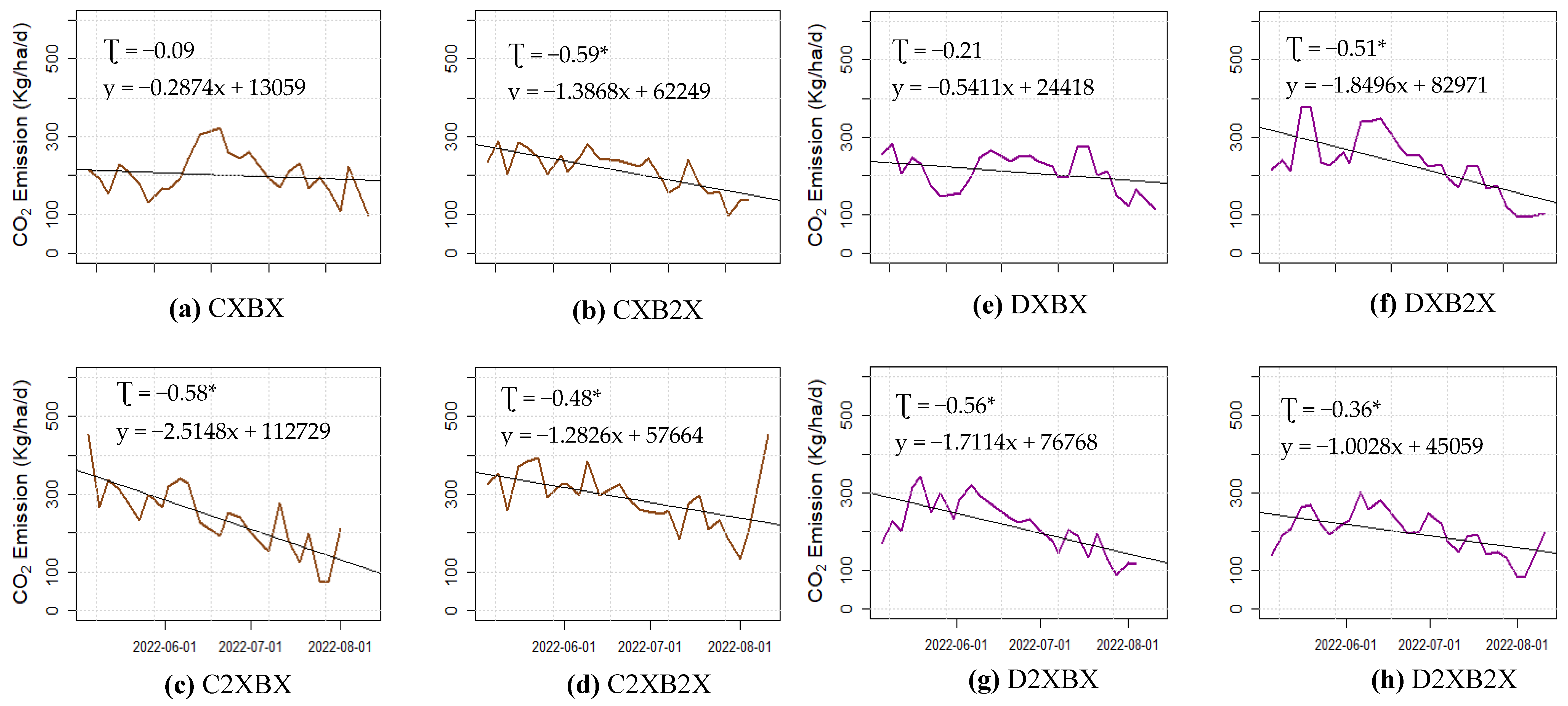
3.2. Short-Term Trends in Soil CO₂ Emissions

The short-term trends in soil CO₂ emissions from all treatments were analyzed using the Mann–Kendall test and linear regression (Figure 7). There was no significant trend in the rate of CO₂ emissions for the control and biochar alone treatment (Figure S1). In the biochar and chicken manure plots, C2XBX showed the highest decreasing trend with a τ value of −0.58, followed by CXB2X. However, the plots with the recommended chicken manure and Level I biochar did not show a significant trend. Similarly, in the case of dairy manure and biochar plots, DXBX showed an insignificant decreasing trend of soil CO₂ emissions. D2XBX showed the highest decreasing trend with a τ value of −0.56. However, CON, BX, and B2X did not show a significantly reducing emission trend over time.

In the case of linear regression analysis, C2XBX and D2XBX showed the highest slope, which is −2.5 and −1.7, respectively. The slope of C2XB2X was higher than that of D2XB2X. The Mann–Kendall and linear regression analyses indicate that C2XBX plots had the highest decreasing trend of soil CO₂ emissions. In general, it is common to observe short-term increases in soil CO₂ emissions after the application of amendments [42,43]. When manure is applied to the soil, promptly available organic matter enhances microbial activity, leading to an increased decomposition rate and subsequent release of CO₂. The chicken and dairy manure used in this study indicated a C/N ratio of 9:1 and 29:1, respectively [11]. Microbes may break down organic matter faster in high carbon levels and limited nitrogen, leading to elevated CO₂ emissions. Over time, the decomposition rate decreases, thereby reducing the emissions [44]. This can be a possible reason for the decreasing trend of soil CO₂ emissions from all of the organically amended plots.

3.3. Effects of Soil Moisture and Thresholds on CO₂ Emissions

(i) Distribution of soil moisture: The daily average soil moisture distribution in the organically amended plots corresponding to the precipitation and irrigation is illustrated in Figure 8. The resulting soil moisture from all of the plots indicates a decreasing pattern starting from the planting date. For example, the control plots showed maximum soil moisture during May, and the minimum values were observed at the end of the season. In the case of biochar-only plots, on average, control plots showed the highest amount of soil moisture content compared to BX and B2X plots (Figure 8a). This could be due to the low uptake of water by plants from control plots [45,46]. The plants in the control plots lacked vigor due to nutrient deficiency compared to those in the biochar-treated plots, indicating less water uptake by plants in the control plots. Also, soil moisture levels at BX plots were higher during the high moisture periods compared to the B2X plots. Meanwhile, B2X showed relatively wetter values toward the middle and end of the growing period. In the case of chicken manure amended plots, all of the plots showed relatively lower soil moisture levels than the control plots. However, double-recommended dairy manure plots showed comparatively higher soil moisture levels at the end of the growing period (Figure 8c).

(ii) Relationship between soil moisture and CO₂ emissions: The results show a strong positive correlation between soil CO₂ and soil moisture level, and the highest correlation is observed for C2XBX plots (r = 0.74, Figure 9). In chicken manure-treated plots, C2XB2X and CXB2X also showed a higher correlation, and the lowest correlation was observed for CXBX (r = 0.32) among the chicken manure plots. Similarly, in the case of dairy plots, DXB2X and D2XBX plots showed a higher correlation. Also, the lowest correlation was observed for DXBX (r = 0.18). Our results indicate that specific impacts of chicken manure, dairy manure, and biochar on soil moisture level and CO₂ emissions can vary depending on application rates.

(iii) Quantifying critical thresholds: A set of critical thresholds associated with soil moisture on CO₂ emissions was quantified using CART. Linear regression assumes and fits one linear model to the entire dataset. However, this may not always be true in real-world datasets. CART can handle non-linear relationships more effectively by splitting the feature space into different regions where the relationship is nearly linear [47]. Also, each decision node in the tree denotes a decision based on a feature value (soil moisture), making it easy to understand how the model arrived at a particular prediction (of soil CO₂ emission). We generated separate decision trees for different organic amendments and their application rate using the CART approach. The model output summarizes the process of estimating different soil moisture thresholds and ranges of soil CO₂ emissions (expressed as a box plot, Figure 10 and Figure 11).

In the case of mixed chicken manure and biochar, C2XBX showed the highest correlation coefficient between soil moisture and CO₂ emissions (Figure 9c). Therefore, the decision tree generated for C2XBX splits into four branches with two thresholds and three outcomes (Figure 10c). Here, the threshold of the first split was 0.133, indicating that if the soil moisture is less than or equal to 0.133 m³m⁻³, the median CO₂ emission is 182 kg ha⁻¹ d⁻¹. Here, p < 0.001 represents the significance of the correlation between the split based on soil moisture and the soil CO₂ emissions from the C2XBX plots. If the soil moisture is greater than 0.133 m³m⁻³, the tree branches toward the right side and provides two outcomes of CO₂ emissions with a soil moisture threshold of 0.235. However, if the soil moisture content is less than or equal to 0.235 m³m⁻³, the median CO₂ emission is 209 kg ha⁻¹ d⁻¹, and if it is higher than 0.235, the median emission is 298 kg ha⁻¹ d⁻¹. For C2XB2X plots, the soil moisture threshold observed was 0.254 m³m⁻³, and if the soil moisture is greater than 0.254 m³m⁻³, the median CO₂ emission is 351 kg ha⁻¹ d⁻¹.

Results of the CART analysis for the mixed dairy and biochar plots showed different soil moisture threshold values (Figure 11) compared to those found in the chicken and biochar plots. For instance, the threshold for the D2XB2X treatment was 0.089 m³m⁻³. If the soil moisture is greater than 0.089 m³m⁻³, the range of CO₂ emissions is high, with a median value of 223 kg ha⁻¹ d⁻¹. In the case of DXB2X, the highest threshold observed was 0.254 m³m⁻³, indicating that if the threshold is higher than 0.254, the median CO₂ emission is 278 kg ha⁻¹ d⁻¹. The chicken manure plots resulted in a higher soil moisture threshold than the dairy manure plots. Overall, the results indicate that a higher rate of organic amendment with higher soil moisture leads to increased CO₂ emissions, especially from the chicken and biochar plots.

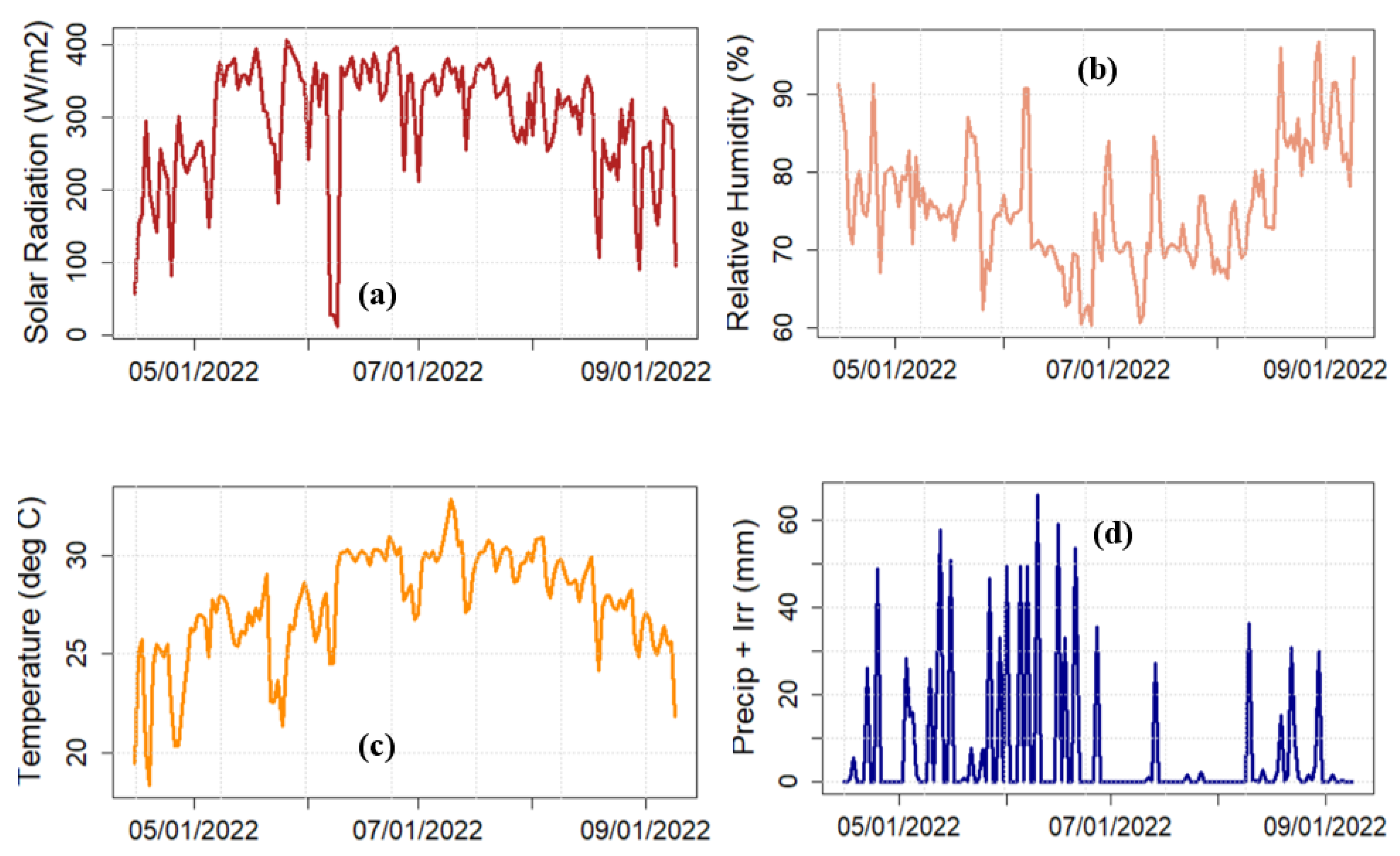
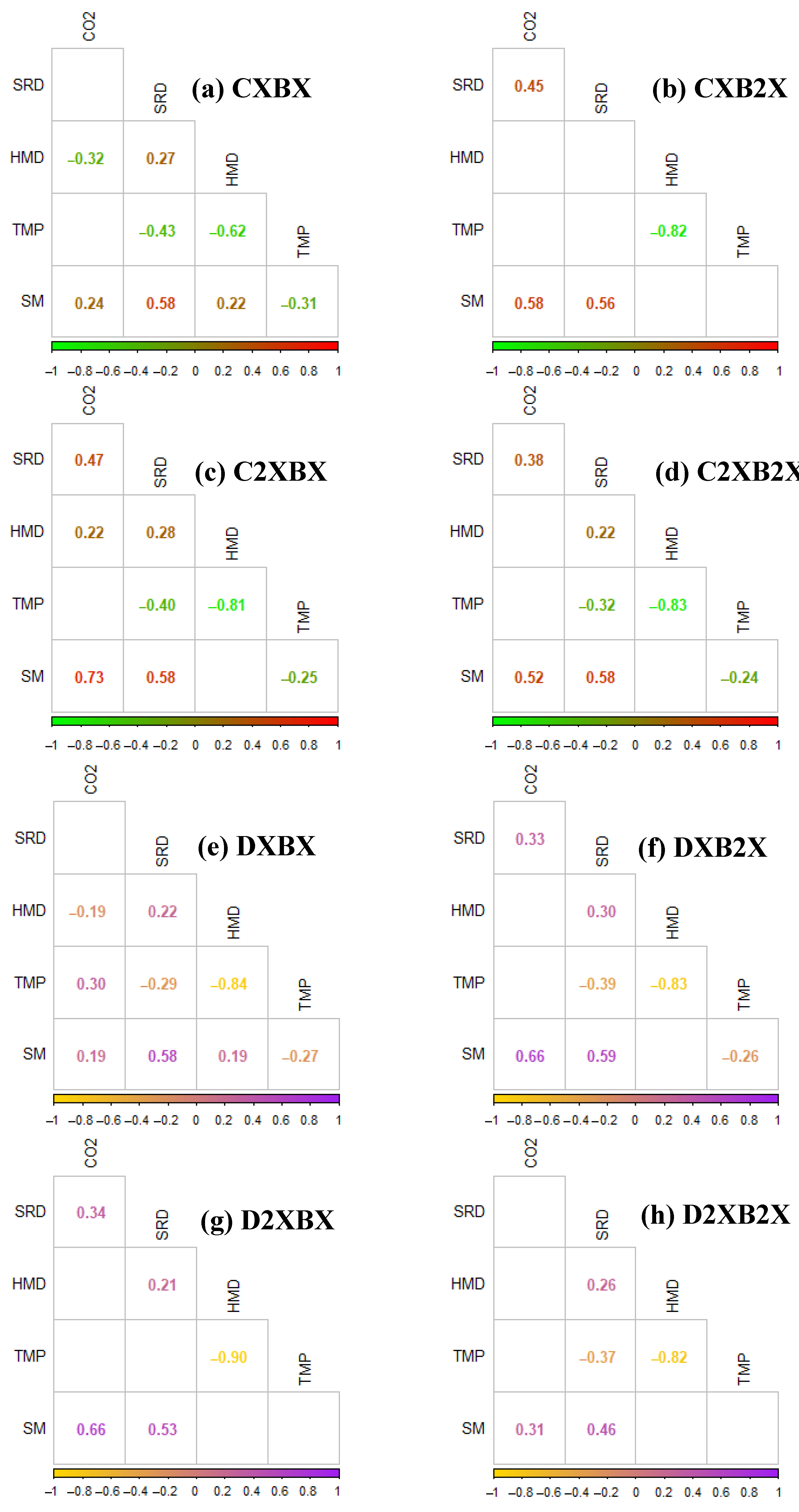
3.4. Potential Impact of Weather Variables on Soil CO₂ Emissions

Air temperature plays a key role in soil CO₂ emissions [16,48]. In general, the rate of CO₂ emissions increases with increasing air temperature. Higher temperatures accelerate microbial activity and enhance the decomposition of organic matter, leading to higher rates of CO₂ release. However, the relationship between air temperature and soil CO₂ emissions is complex and can be influenced by several factors, such as soil organic amendments type and rate [16]. In this study, we considered relative humidity (HMD) and solar radiation (SRD) in addition to the air temperature (TMP) and quantified their relationship with soil CO₂ emissions using machine learning applications. Figure 12 illustrates the Pearson correlation between soil CO₂ emissions and TMP, HMD, SRD, and soil moisture (SM) in a correlation matrix. Here, the weather variables for the analysis were selected based on the CO₂ measurement time.

Like air temperature, SRD can lead to higher soil temperatures, thus increasing the rate of microbial activity and subsequent CO₂ emissions. A higher SRD leads to increased photosynthesis, affecting the amount of carbon added to the soil through root exudation. The correlation matrix also indicates the interdependence among the weather variables. For example, HMD and TMP showed a negative correlation in our analysis. TMP and SRD showed a positive correlation between CO₂ emissions in most of the plots, indicating that a higher TMP/SRD leads to increased emissions.

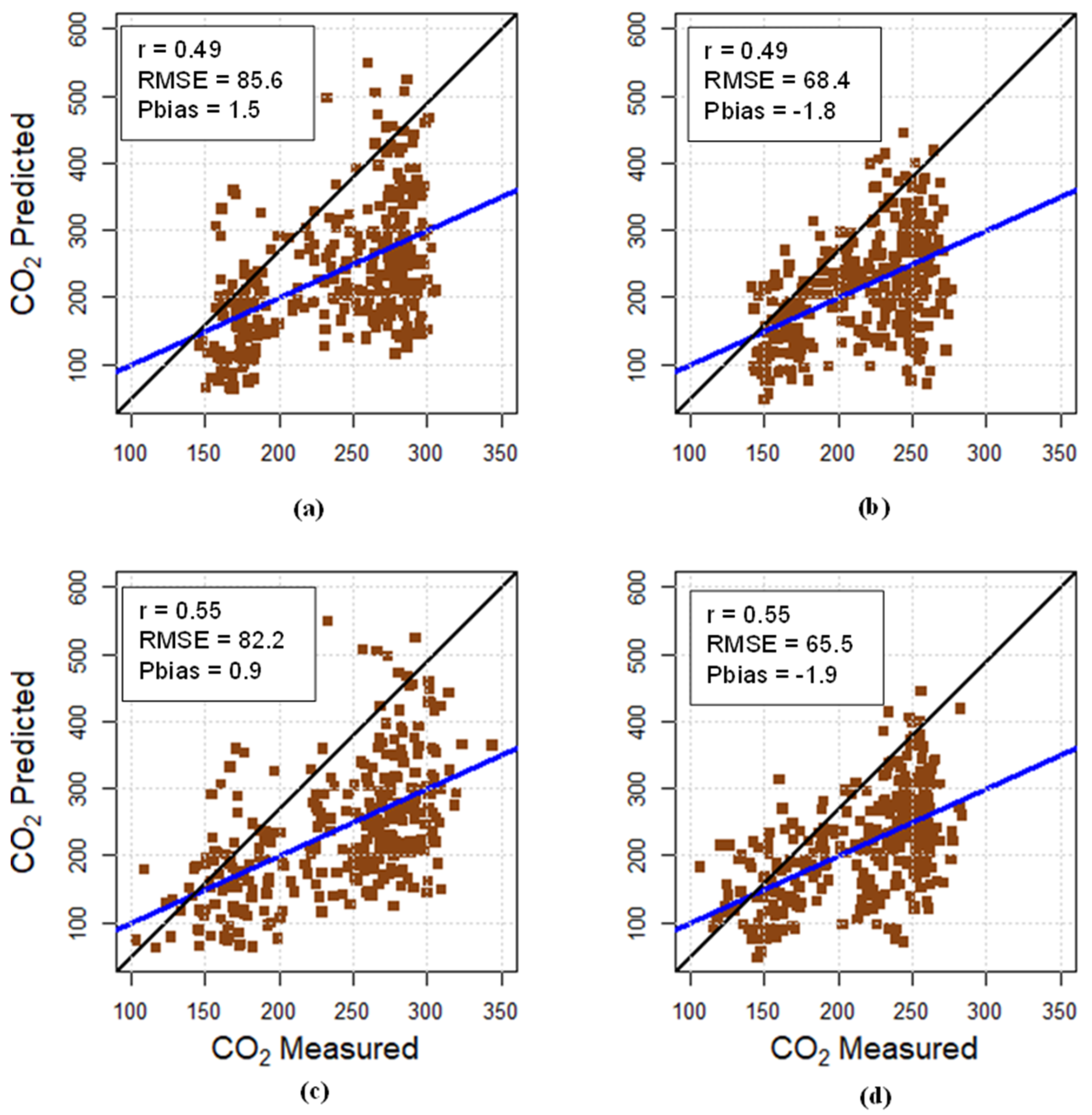
3.5. Predicting Soil CO₂ Emissions Using Weather Variables and Soil Moisture

This study utilized multilinear regression (MLR) and generalized additive models (GAMs) to predict soil CO₂ emissions for different amendment types and rates, incorporating weather variables and soil moisture as predictors. The findings demonstrate that GAMs outperformed MLR. For instance, in the case of the CXBX amendment, MLR yielded a Pearson correlation of 0.51 and an RMSE of 71.4 kg ha⁻¹d⁻¹, whereas GAMs exhibited an r-value of 0.62 and an RMSE of 65.2 kg ha⁻¹d⁻¹. Similarly, for the mixed chicken and biochar amendment, the highest performance was observed for CXB2X in GAMs based on the lowest RMSE value, with an r-value of 0.75 and an RMSE value of 43.4 kg ha⁻¹ d⁻¹. We also assessed how well MLR and GAMs predict soil CO₂ emissions for plots amended with chicken and dairy manure separately (Figure 13). The training and testing of MLR and GAMs were performed to evaluate model performance (Table S1). GAMs and MLR showed a Pearson correlation of 0.55 between the measured and predicted soil CO₂ emissions. The PBIAS was very low for all of the developed models. GAMs generated for chicken manure plots showed the lowest PBIAS value.

To evaluate the modeling results, we compared their goodness-of-fit statistics with recent research from similar studies. A random forest study in the semi-arid U.S. achieved a coefficient of determination of 0.68 for CO₂ flux prediction [49]. The process-based DNDC model, validated against Irish pasture and arable sites, reproduced cumulative soil respiration with an R² value of 0.60 and RMSE of 1.8 kg C ha⁻¹ d⁻¹ [50]. These cross-study comparisons underscore that the lightweight, data-driven approaches presented herein match similar research.

3.6. Potentials and Limitations

Although the study was designed for a single crop growing season, limiting its capacity to account for multi-annual variability in weather and soil moisture patterns, the high-resolution data and detailed insights provide a robust foundation for future research. The observed relationship between soil moisture, amendment effects, and CO₂ emissions might not fully represent long-term trends. However, the study deeply explains soil moisture dynamics and their relationship with CO₂ emissions under specific weather and amendment conditions using machine learning applications, including CART. In addition, the research formulated a method to predict short-term soil CO₂ emissions using weather variables and plot-measured soil moisture by applying MLR and GAMs. Seasonal anomalies or specific climatic events during the study period may impact soil CO₂ emissions, limiting the long-term applicability of the derived thresholds and predictive models. Future research incorporating multiple seasons that reflect diverse environmental conditions will be essential to validate and refine these initial insights for broader implementation. A potential limitation of this study is that it did not include the analysis of crop biomass or yield, which are critical indicators of agricultural productivity, as this was considered out of scope. Additionally, the study could be enhanced by including measurements of nitrous oxide (N₂O) and methane (CH₄) emissions, providing a broader understanding of GHG fluxes in agricultural systems. Overall, the findings from this study set a valuable benchmark that subsequent multi-season studies can build upon to explore longer-term variability and further refine predictive models.

4. Conclusions

This study quantified the sustainability implications of soil moisture and weather variables on soil CO₂ emissions from climate-smart agricultural practices by applying CART, multilinear regression, and Generalized Additive Models. This study used three rates (0, recommended, and double recommended) of chicken and dairy manure and two biochar levels (Level I and II) to elucidate the impact of soil CO₂ emissions under sweet corn crops in the southeast Texas environment. The soil type in the study area is Wockley fine sandy loam with Surface samples (0–18 cm) containing 61–70% sand, 26–32% silt, and 4–7% clay, grading to a sandy-clay-loam subsoil, and total organic C at the start of the study averaged 0.50% (3.5 g kg⁻¹). Also, the average hydraulic conductivity is measured as 0.97 cm hr⁻¹. These metrics justify the importance of quantifying the soil CO₂ flux in relation to soil water availability.

The proposed framework can predict soil moisture thresholds corresponding to soil CO₂ emissions, providing insights for sustainable soil management. Also, an extensive comparison between multilinear regression and a generalized additive model was performed to predict soil CO₂ emissions by splitting the data into training and test sets and by evaluating different goodness-of-fit statistics. The following conclusions are drawn from our sustainability-focused soil analysis.

(a)

The Level II rate of biochar (B2X) reduced soil CO₂ emissions by 14.5% compared to the control plots. The maximum soil CO₂ emissions were observed from the double recommended chicken manure and the Level II biochar (C2XB2X) plots, indicating that mixing biochar with chicken manure failed to reduce soil CO₂ emissions. Also, mixing biochar with dairy/chicken manure showed a decreasing trend of CO₂ emissions over time. For example, C2XB2X showed a tau value of −0.48 in the Mann–Kendall trend analysis.

(b)

The presence of soil organic amendments enhanced nutrient availability and plant growth, leading to increased crop water demand. As a result, the plants in the organically amended plots might have consumed more water, contributing to more efficient resource use but also reducing the soil moisture content compared to the control fields.

(c)

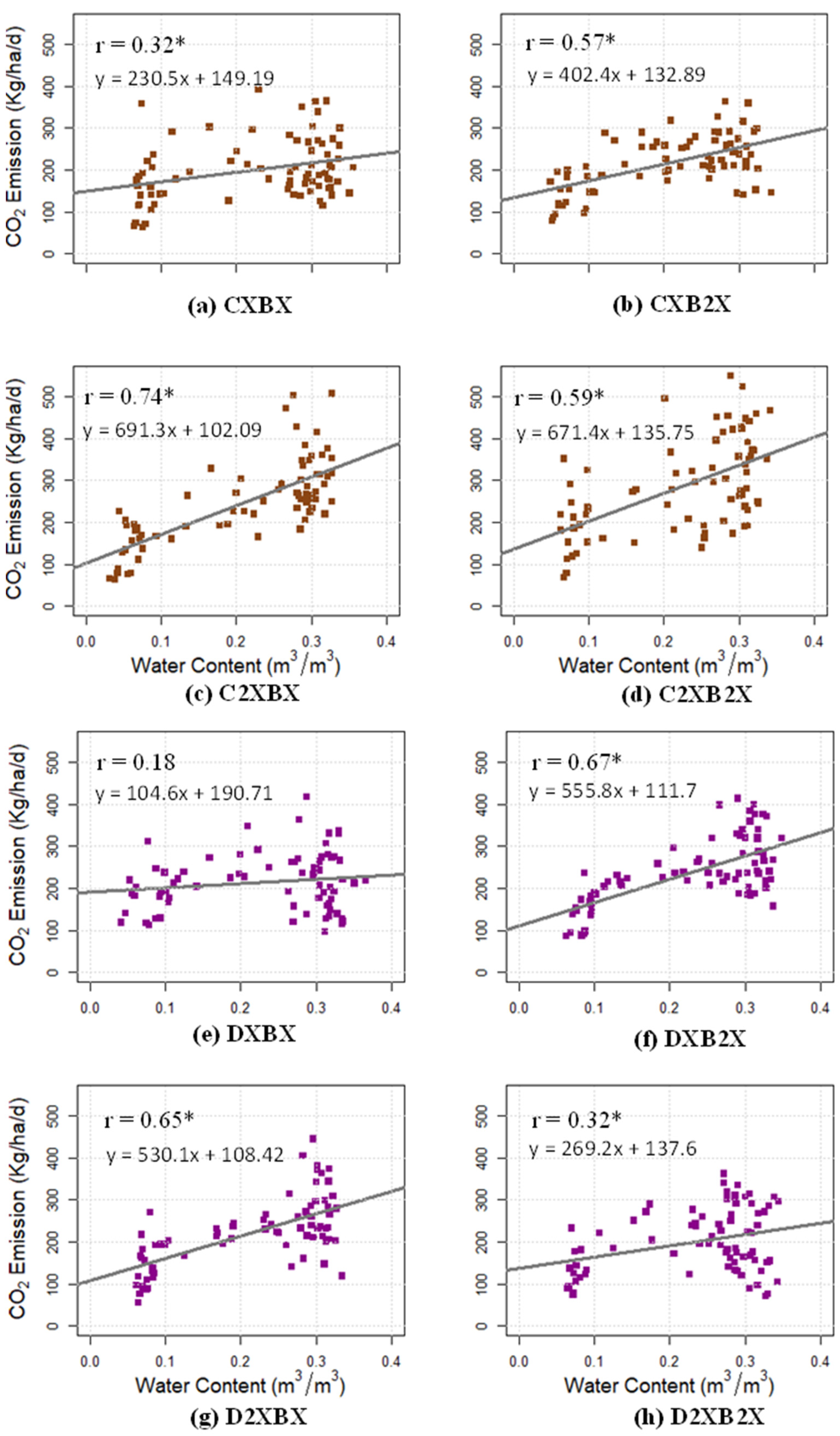
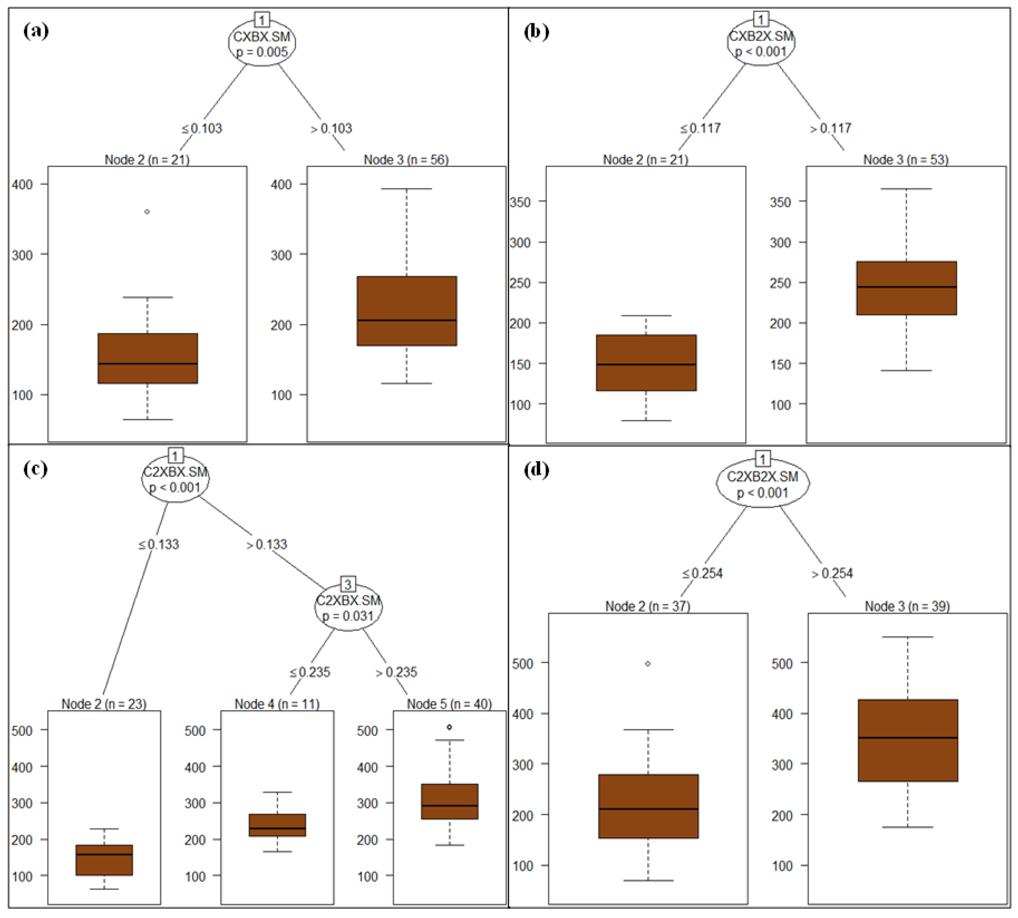
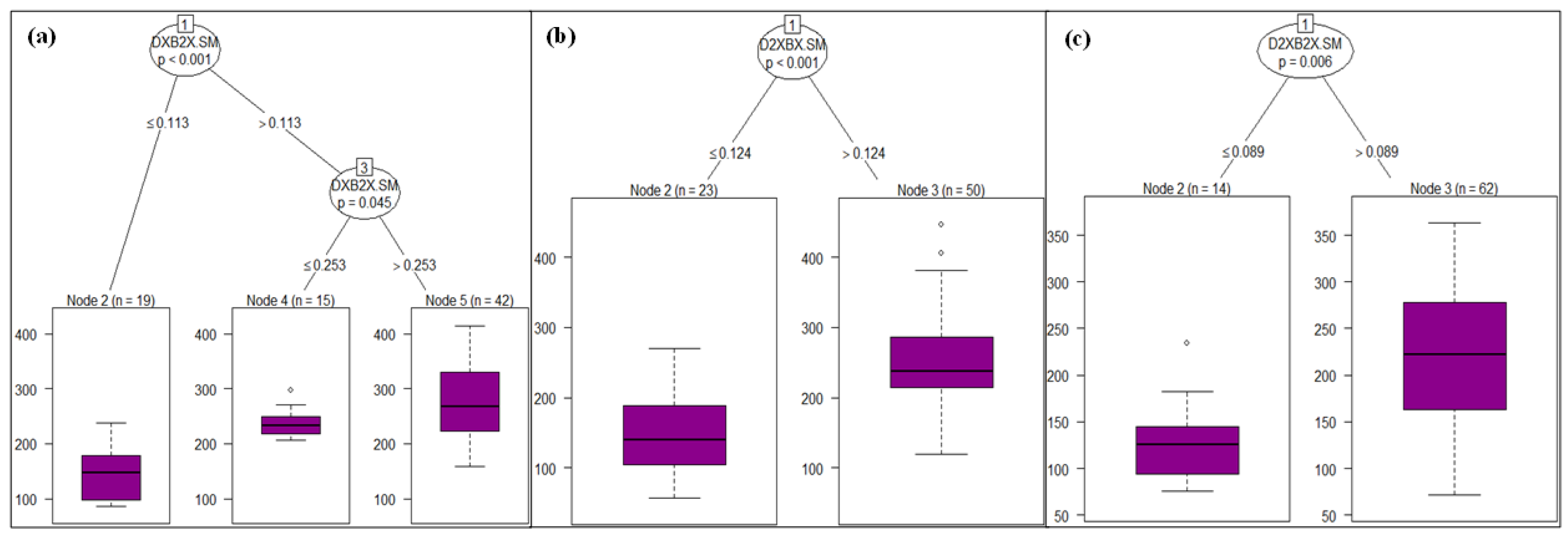
The soil moisture levels significantly correlated with soil CO₂ emissions from most organically amended plots. The highest correlation was observed for double-recommended chicken and the Level I biochar plots (C2XBX). The decision tree approach applied in this study quantified critical thresholds of soil moisture corresponding to soil CO₂ emissions. In the case of C2XBX, the soil moisture threshold identified was 0.133 m³m⁻³, indicating that soil moisture higher than 0.133 m³m⁻³ leads to higher soil CO₂ emissions from C2XBX plots. In predicting soil CO₂, GAMs outperformed MLR across all organic amendment types and rates.

References

1. Shahzad, A.; Ullah, S.; Dar, A.A.; Sardar, M.F.; Mehmood, T.; Tufail, M.A.; Shakoor, A.; Haris, M. Nexus on Climate Change: Agriculture and Possible Solution to Cope Future Climate Change Stresses. Environ. Sci. Pollut. Res. 2021, 28, 14211–14232. [Google Scholar] [CrossRef] [PubMed]
2. Lipper, L.; Thornton, P.; Campbell, B.M.; Baedeker, T.; Braimoh, A.; Bwalya, M.; Caron, P.; Cattaneo, A.; Garrity, D.; Henry, K.; et al. Climate-Smart Agriculture for Food Security. Nat. Clim. Chang. 2014, 4, 1068–1072. [Google Scholar] [CrossRef]
3. Lobell, D.B.; Schlenker, W.; Costa-Roberts, J. Climate Trends and Global Crop Production since 1980. Science 2011, 333, 616–620. [Google Scholar] [CrossRef] [PubMed]
4. Battisti, D.S.; Naylor, R.L. Historical Warnings of Future Food Insecurity with Unprecedented Seasonal Heat. Science 2009, 323, 240–244. [Google Scholar] [CrossRef]
5. Smith, P.; Bustamante, M.; Ahammad, H.; Clark, H.; Dong, H.; Elsiddig, E.A.; Haberl, H.; Harper, R.; House, J.; Jafari, M. Agriculture, Forestry and Other Land Use (AFOLU). In Climate Change 2014: Mitigation of Climate Change. Contribution of Working Group III to the Fifth Assessment Report of the Intergovernmental Panel on Climate Change; Cambridge University Press: Cambridge, UK, 2014; pp. 811–922. [Google Scholar]
6. Wollenberg, E.; Richards, M.; Smith, P.; Havlík, P.; Obersteiner, M.; Tubiello, F.N.; Herold, M.; Gerber, P.; Carter, S.; Reisinger, A.; et al. Reducing Emissions from Agriculture to Meet the 2 °C Target. Glob. Change Biol. 2016, 22, 3859–3864. [Google Scholar] [CrossRef]
7. Solazzo, E.; Galmarini, S. Error Apportionment for Atmospheric Chemistry-Transport Models—A New Approach to Model Evaluation. Atmos. Chem. Phys. 2016, 16, 6263–6283. [Google Scholar] [CrossRef]
8. FAO. “Climate-Smart” Agriculture: Policies, Practices and Financing for Food Security, Adaption and Mitigation; Food and Agriculture Organization of the United Nations: Rome, Italy, 2010; ISBN 9251011745. [Google Scholar]
9. NASS. 2022 Census of Agriculture; NASS: Beijing, China, 2022.
10. Fares, A.; Bensley, A.; Bayabil, H.; Awal, R.; Fares, S.; Valenzuela, H.; Abbas, F. Carbon Dioxide Emission in Relation with Irrigation and Organic Amendments from a Sweet Corn Field. J. Environ. Sci. Health Part B 2017, 52, 387–394. [Google Scholar] [CrossRef]
11. Veettil, A.V.; Rahman, A.; Awal, R.; Fares, A.; Melaku, N.D.; Thapa, B.; Elhassan, A.; Woldesenbet, S. Transforming Soil: Climate-Smart Amendments Boost Soil Physical and Hydrological Properties. Soil Syst. 2024, 8, 134. [Google Scholar] [CrossRef]
12. Imran, M.A.; Ali, A.; Culas, R.J.; Ashfaq, M.; Baig, I.A.; Nasir, S.; Hashmi, A.H. Sustainability and efficiency analysis wrt adoption of climate-smart agriculture (CSA) in Pakistan: A group-wise comparison of adopters and conventional farmers. Environ. Sci. Pollut. Res. 2022, 29, 19337–19351. [Google Scholar] [CrossRef]
13. Fares, A.; Abbas, F.; Ahmad, A.; Deenik, J.L.; Safeeq, M. Response of Selected Soil Physical and Hydrologic Properties to Manure Amendment Rates, Levels, Andtypes. Soil Sci. 2008, 173, 522–533. [Google Scholar] [CrossRef]
14. Chadwick, D.; Sommer, S.; Thorman, R.; Fangueiro, D.; Cardenas, L.; Amon, B.; Misselbrook, T. Manure Management: Implications for Greenhouse Gas Emissions. Anim. Feed Sci. Technol. 2011, 166–167, 514–531. [Google Scholar] [CrossRef]
15. Liu, X.; Wang, S.; Zhuang, Q.; Jin, X.; Bian, Z.; Zhou, M.; Meng, Z.; Han, C.; Guo, X.; Jin, W.; et al. A review on carbon source and sink in arable land ecosystems. Land 2022, 11, 580. [Google Scholar] [CrossRef]
16. Hamrani, A.; Akbarzadeh, A.; Madramootoo, C.A. Machine Learning for Predicting Greenhouse Gas Emissions from Agricultural Soils. Sci. Total Environ. 2020, 741, 140338. [Google Scholar] [CrossRef] [PubMed]
17. González Costa, J.J.; Reigosa, M.J.; Matías, J.M.; Covelo, E.F. Soil Cd, Cr, Cu, Ni, Pb and Zn Sorption and Retention Models Using SVM: Variable Selection and Competitive Model. Sci. Total Environ. 2017, 593–594, 508–522. [Google Scholar] [CrossRef]
18. Pham, B.T.; Nguyen, M.D.; Van Dao, D.; Prakash, I.; Ly, H.B.; Le, T.T.; Ho, L.S.; Nguyen, K.T.; Ngo, T.Q.; Hoang, V.; et al. Development of Artificial Intelligence Models for the Prediction of Compression Coefficient of Soil: An Application of Monte Carlo Sensitivity Analysis. Sci. Total Environ. 2019, 679, 172–184. [Google Scholar] [CrossRef]
19. Schaufler, G.; Kitzler, B.; Schindlbacher, A.; Skiba, U.; Sutton, M.A.; Zechmeister-Boltenstern, S. Greenhouse Gas Emissions from European Soils under Different Land Use: Effects of Soil Moisture and Temperature. Eur. J. Soil Sci. 2010, 61, 683–696. [Google Scholar] [CrossRef]
20. Zhang, Y.; Hou, W.; Chi, M.; Sun, Y.; An, J.; Yu, N.; Zou, H. Simulating the Effects of Soil Temperature and Soil Moisture on CO2 and CH4 Emissions in Rice Straw-Enriched Paddy Soil. CATENA 2020, 194, 104677. [Google Scholar] [CrossRef]
21. Keiluweit, M.; Wanzek, T.; Kleber, M.; Nico, P.; Fendorf, S. Anaerobic Microsites Have an Unaccounted Role in Soil Carbon Stabilization. Nat. Commun. 2017, 8, 1771. [Google Scholar] [CrossRef]
22. Batson, J.; Noe, G.B.; Hupp, C.R.; Krauss, K.W.; Rybicki, N.B.; Schenk, E.R. Soil Greenhouse Gas Emissions and Carbon Budgeting in a Short-Hydroperiod Floodplain Wetland. J. Geophys. Res. Biogeosci. 2015, 120, 77–95. [Google Scholar] [CrossRef]
23. Tanha, M.; Mohtar, R.H.; Assi, A.T.; Awal, R.; Fares, A. Soil Hydrostructural Parameters under Various Soil Management Practices. Agric. Water Manag. 2024, 292, 108633. [Google Scholar] [CrossRef]
24. Awal, R.; Fares, A.; Habibi, H. Irrigation Scheduling Tools: IrrigWise and IrrigWise-PRISM for Agricultural Crops and Urban Landscapes. In Proceedings of the 6th Decennial National Irrigation Symposium, San Diego, CA, USA, 6–8 December 2021. [Google Scholar] [CrossRef]
25. Mittelbach, H.; Lehner, I.; Seneviratne, S.I. Comparison of Four Soil Moisture Sensor Types under Field Conditions in Switzerland. J. Hydrol. 2012, 430–431, 39–49. [Google Scholar] [CrossRef]
26. Spelman, D.; Kinzli, K.-D.; Kunberger, T. Calibration of the 10HS Soil Moisture Sensor for Southwest Florida Agricultural Soils. J. Irrig. Drain. Eng. 2013, 139, 965–971. [Google Scholar] [CrossRef]
27. Mann, H.B. Nonparametric Tests Against Trend. Econometrica 1945, 13, 245–249. [Google Scholar] [CrossRef]
28. Bzdok, D.; Krzywinski, M.; Altman, N. Machine Learning: A Primer. Nat. Methods 2017, 14, 1119–1120. [Google Scholar] [CrossRef]
29. James, G.; Witten, D.; Hastie, T.; Tibshirani, R. An Introduction to Statistical Learning; Springer: Berlin/Heidelberg, Germany, 2013; Volume 112. [Google Scholar]
30. Pekel, E. Estimation of soil moisture using decision tree regression. Theor. Appl. Climatol. 2020, 139, 1111–1119. [Google Scholar] [CrossRef]
31. Hothorn, T.; Hornik, K.; Strobl, C.; Zeileis, A. Party: A Laboratory for Recursive Partytioning. 2010. Available online: https://cran.r-project.org/web/packages/party/vignettes/party.pdf (accessed on 30 June 2025).
32. Guo, M.; He, Z.; Uchimiya, S.M. Introduction to Biochar as an Agricultural and Environmental Amendment. In Agricultural and Environmental Applications of Biochar: Advances and Barriers; Soil Science Society of America, Inc.: Madison, WI, USA, 2015; pp. 1–14. [Google Scholar] [CrossRef]
33. Gascó, G.; Paz-Ferreiro, J.; Cely, P.; Plaza, C.; Méndez, A. Influence of Pig Manure and Its Biochar on Soil CO2 Emissions and Soil Enzymes. Ecol. Eng. 2016, 95, 19–24. [Google Scholar] [CrossRef]
34. Sohi, S.P.; Krull, E.; Lopez-Capel, E.; Bol, R. A Review of Biochar and Its Use and Function in Soil. Adv. Agron. 2010, 105, 47–82. [Google Scholar] [CrossRef]
35. Lehmann, J.; Cowie, A.; Masiello, C.A.; Kammann, C.; Woolf, D.; Amonette, J.E.; Cayuela, M.L.; Camps-Arbestain, M.; Whitman, T. Biochar in Climate Change Mitigation. Nat. Geosci. 2021, 14, 883–892. [Google Scholar] [CrossRef]
36. Jeffery, S.; Abalos, D.; Prodana, M.; Bastos, A.C.; Van Groenigen, J.W.; Hungate, B.A.; Verheijen, F. Biochar Boosts Tropical but Not Temperate Crop Yields. Environ. Res. Lett. 2017, 12, 053001. [Google Scholar] [CrossRef]
37. Luo, L.; Wang, J.; Lv, J.; Liu, Z.; Sun, T.; Yang, Y.; Zhu, Y.G. Carbon Sequestration Strategies in Soil Using Biochar: Advances, Challenges, and Opportunities. Environ. Sci. Technol. 2023, 57, 11357–11372. [Google Scholar] [CrossRef]
38. Lorenz, K.; Lal, R. Biochar Application to Soil for Climate Change Mitigation by Soil Organic Carbon Sequestration. J. Plant Nutr. Soil Sci. 2014, 177, 651–670. [Google Scholar] [CrossRef]
39. Zheng, X.; Xu, W.; Dong, J.; Yang, T.; Shangguan, Z.; Qu, J.; Li, X.; Tan, X. The Effects of Biochar and Its Applications in the Microbial Remediation of Contaminated Soil: A Review. J. Hazard. Mater. 2022, 438, 129557. [Google Scholar] [CrossRef] [PubMed]
40. Cross, A.; Sohi, S.P. A Method for Screening the Relative Long-Term Stability of Biochar. GCB Bioenergy 2013, 5, 215–220. [Google Scholar] [CrossRef]
41. Sistani, K.R.; Simmons, J.R.; Jn-Baptiste, M.; Novak, J.M. Poultry Litter, Biochar, and Fertilizer Effect on Corn Yield, Nutrient Uptake, N2O and CO2 Emissions. Environments 2019, 6, 55. [Google Scholar] [CrossRef]
42. Galvez, A.; Sinicco, T.; Cayuela, M.L.; Mingorance, M.D.; Fornasier, F.; Mondini, C. Short Term Effects of Bioenergy By-Products on Soil C and N Dynamics, Nutrient Availability and Biochemical Properties. Agric. Ecosyst. Environ. 2012, 160, 3–14. [Google Scholar] [CrossRef]
43. Ameloot, N.; De Neve, S.; Jegajeevagan, K.; Yildiz, G.; Buchan, D.; Funkuin, Y.N.; Prins, W.; Bouckaert, L.; Sleutel, S. Short-Term CO2 and N2O Emissions and Microbial Properties of Biochar Amended Sandy Loam Soils. Soil Biol. Biochem. 2013, 57, 401–410. [Google Scholar] [CrossRef]
44. Shahbaz, M.; Kuzyakov, Y.; Sanaullah, M.; Heitkamp, F.; Zelenev, V.; Kumar, A.; Blagodatskaya, E. Microbial Decomposition of Soil Organic Matter Is Mediated by Quality and Quantity of Crop Residues: Mechanisms and Thresholds. Biol. Fertil. Soils 2017, 53, 287–301. [Google Scholar] [CrossRef]
45. Butler, T.J.; Muir, J.P. Dairy Manure Compost Improves Soil and Increases Tall Wheatgrass Yield. Agron. J. 2006, 98, 1090–1096. [Google Scholar] [CrossRef]
46. Jannoura, R.; Joergensen, R.G.; Bruns, C. Organic Fertilizer Effects on Growth, Crop Yield, and Soil Microbial Biomass Indices in Sole and Intercropped Peas and Oats under Organic Farming Conditions. Eur. J. Agron. 2014, 52, 259–270. [Google Scholar] [CrossRef]
47. Veettil, A.V.; Mishra, A.K. Quantifying Thresholds for Advancing Impact-Based Drought Assessment Using Classification and Regression Tree (CART) Models. J. Hydrol. 2023, 625, 129966. [Google Scholar] [CrossRef]
48. Ren, W.; Banger, K.; Tao, B.; Yang, J.; Huang, Y.; Tian, H. Global Pattern and Change of Cropland Soil Organic Carbon during 1901–2010: Roles of Climate, Atmospheric Chemistry, Land Use and Management. Geogr. Sustain. 2020, 1, 59–69. [Google Scholar] [CrossRef]
49. Bista, P.; Shakya, S.R.; Acharya, P.; Ghimire, R. Evaluating machine learning models for greenhouse gas emissions prediction in diversified semi-arid cropping systems. Soil Sci. Soc. Am. J. 2025, 89, e70057. [Google Scholar] [CrossRef]
50. Abdalla, M.; Kumar, S.; Jones, M.; Burke, J.; Williams, M. Testing DNDC model for simulating soil respiration and assessing the effects of climate change on the CO2 gas flux from Irish agriculture. Glob. Planet. Chang. 2011, 78, 106–115. [Google Scholar] [CrossRef]
Figure 1. The experimental and machine learning framework for quantifying the impact of soil moisture and temperature on soil CO2 emissions from sweet corn agricultural systems.
Sustainability 17 06101 g001
Figure 2. The location of experimental plots at PVAMU Research Farm. The plots’ layout includes three replications, treatment types, and treatment rates.
Sustainability 17 06101 g002
Figure 3. A view of the experimental setup. (a) Soil moisture data logger, (b) LI-8100A (LI-COR Biosciences, Lincoln, NE, USA) survey system, and (c) a view of the experimental plots during the middle of the growing season. The effect of organic amendments on sweet corn can be visually interpreted from (c).
Sustainability 17 06101 g003
Figure 4. Temporal distribution of (a) solar radiation, (b) relative humidity, (c) temperature, and (d) the sum of precipitation and supplementary irrigation during the experimental period.
Sustainability 17 06101 g004
Figure 5. (a) Effect of biochar rate at Level I and Level II on soil CO2 emissions. (b) Effect of manure type (chicken and dairy manure) on soil CO2 emissions. (c) Effects of amendment rates on soil CO2 emissions. Here, 2×Recommended is the double recommended rate of manure.
Sustainability 17 06101 g005
Figure 6. Boxplot showing the soil CO2 emissions from each treatment type. The C2XB2X showed the highest range and median of CO2 emissions during the experimental period. For the plot design, we used C0BX and D0BX, considered BX, and C0B2X and D0B2X are considered B2X in the analysis.
Sustainability 17 06101 g006
Figure 7. Time series of soil CO2 emissions from organic amendment plots with the Mann–Kendall trend. Ʈ is positive when the trend increases and negative when the trend decreases. The p-value indicates the significance of the trend (* indicates the significance, p < 0.05).
Sustainability 17 06101 g007
Figure 8. Time series of soil moisture (m3m−3) for (a) biochar amended plots, (b) mixed chicken manure and biochar amended plots, and (c) mixed dairy manure and biochar amended plots. Soil moisture values are averages across three replicates. Precipitation + irrigation during the growing season is also illustrated here.
Sustainability 17 06101 g008
Figure 9. Scatter plot showing the correlation between soil water content and soil CO2 emissions from chicken and dairy manure plots (* indicates the significance, p < 0.05).
Sustainability 17 06101 g009
Figure 10. Decision tree showing the threshold of soil water content for chicken manure-treated fields: (a) CXBX; (b) CXB2X; (c) C2XBX; (d) C2XB2X. The box plot shows the soil CO2 emissions from each treatment corresponding to the soil moisture threshold.
Sustainability 17 06101 g010
Figure 11. Decision tree showing the threshold of soil water content for dairy manure-treated fields: (a) DXB2X; (b) D2XBX; (c) D2XB2X. The box plot shows the soil CO2 emissions from each treatment corresponding to the soil moisture threshold.
Sustainability 17 06101 g011
Figure 12. The correlation matrix shows the Pearson correlation (r) between soil moisture, weather variables, and CO2 emissions from chicken and dairy manure plots. Correlation values are only shown for a significance level of p < 0.05.
Sustainability 17 06101 g012
Figure 13. The scatter plot shows the correlation between predicted and measured soil CO2 emissions from the (a) chicken and (b) dairy manure plots based on MLR and (c) chicken and (d) dairy manure plots based on GAMs.
Sustainability 17 06101 g013