1. Introduction
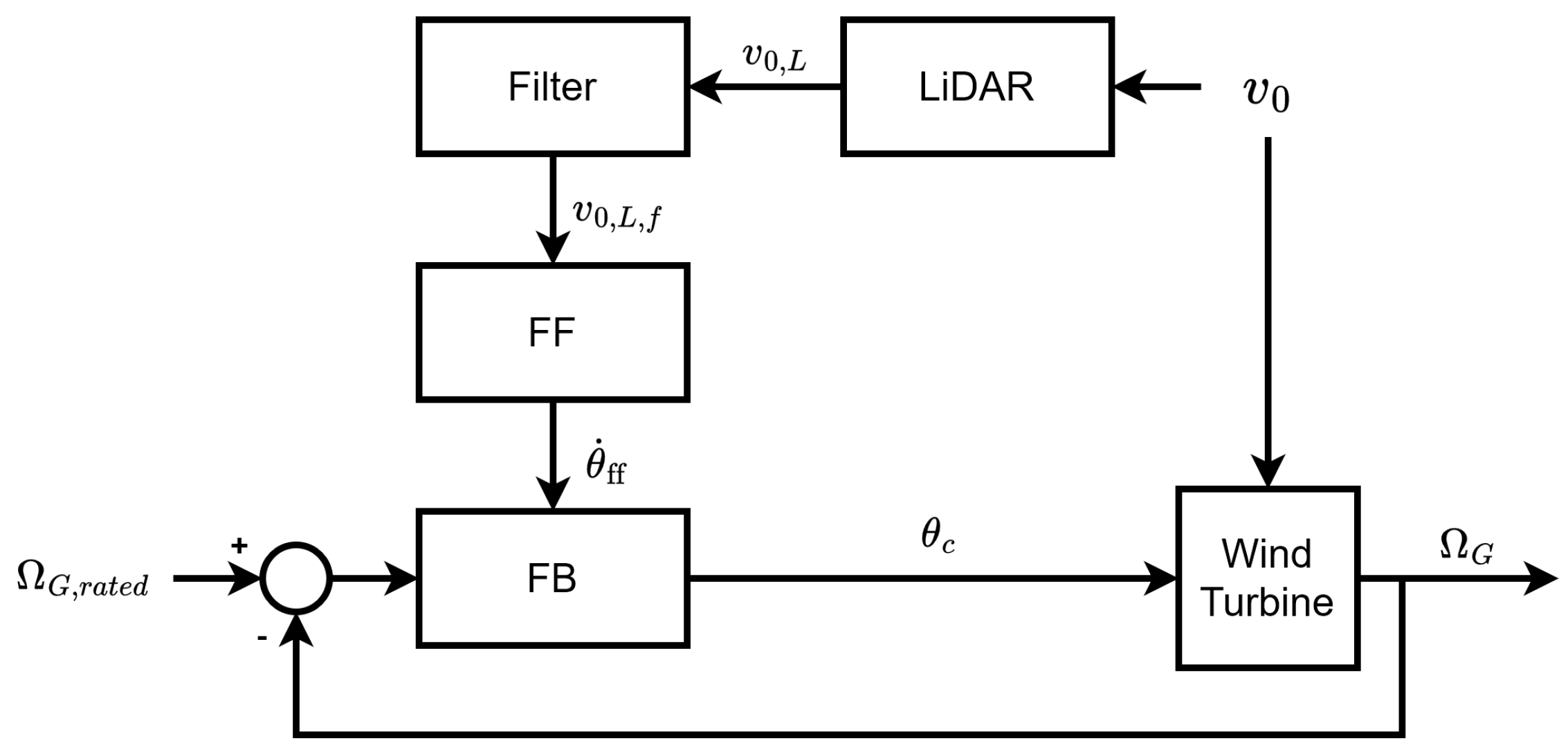
As wind turbines increase in size, different control solutions are utilized to limit the structural loads. Nevertheless, one of the challenges when designing control systems for wind turbines is that the controller action happens after the wind inflow hits the turbine, which is known as the feedback mechanism. Feedforward control can overcome the challenge but it requires the knowledge of the incoming wind speed. The wind speed, generally obtained from nacelle-mounted anemometers, is disturbed by the rotor and only represents one point of measurement across the rotor. The application of Light Detection And Ranging (LiDAR) system technology for measuring upstream wind speed has shown promise in wind turbine control as it can remotely measure the velocity of the particles in the air, enabling estimation of the wind speed at a specific upstream distance from the wind turbine. These measurements then can be used to plan a control action to reduce structural fatigue loads and improve rotor speed regulation. Therefore, the advancement in LiDAR systems has motivated the study of LiDAR-assisted control for wind turbines.
One of the pioneering investigations into LiDAR-assisted feedforward control was undertaken by Harris et al. [
1]. After this, a growing body of research has employed LiDAR systems to enhance collective pitch control, with the objective of refining rotor speed regulation and mitigating fatigue load, as documented in [
2]. Moreover, various studies, such as [
3], have concentrated on leveraging LiDAR technology for enhancing individual pitch control, thereby mitigating loads on blades and other turbine structures. Some research (e.g., [
4]), has utilized LiDARs to optimize turbine power capture. In addition, the findings presented in [
5,
6] demonstrated the integration of wind measurements into a model predictive control (MPC) framework, resulting in enhanced load alleviation. In recent years, a few studies, including [
7,
8], have investigated the benefits of LiDAR-assisted control under varying turbulence conditions. Two further studies [
9,
10] explored LiDAR-assisted control retrofit applications, where LiDAR measurements were used to modify the rotor speed signal rather than directly influencing the pitch angle. Another study [
11] examined LAC for floating wind turbines, while [
12] applied a nonlinear output regulation approach to LiDAR-assisted control.
Numerous full-scale tests, including those outlined in [
13], have been conducted to showcase and validate the efficacy of LiDAR-assisted control. More recently, an International Energy Agency (IEA) Wind task was established to endorse the adoption of LiDAR technology in wind energy applications, as highlighted in [
14,
15].
However, there is still a research gap. First, the applicability of current commercially available fixed-beam LiDAR systems in larger wind turbines has some potential limitations. Second, different feedforward control strategies would affect the benefit of using LiDARs in wind turbine control. The performance of two well-known LiDAR-assisted feedforward control approaches, developed by Schlipf [
16] and Bossanyi [
17] is evaluated, particularly regarding their implementation and uncertainties in the mapping between the wind speed to pitch angle used in the feedforward controller.
Therefore, the objective of this study is twofold: (i) to investigate how the coherence of the LiDAR-estimated rotor effective wind speed is influenced by the LiDAR configuration—specifically the number of beams, their measurement locations, and the resolution of the turbulence box; and (ii) to conduct a detailed analysis of two well-known feedforward LiDAR-assisted control approaches, namely those proposed by Schlipf [
16] and Bossanyi [
17]. Building on the simulation framework from our previous work [
18], we extend that work significantly in both scope and analysis. In particular, this study examines variations in LiDAR configurations and coherence across different wind turbine sizes, the resulting effects on load reduction, and how the feedback control design influences both reference LiDAR-assisted strategies.
Wind energy plays a central role in the global transition towards a more sustainable and low-carbon energy system. This study contributes to that objective by investigating advanced control strategies that enable more efficient and reliable operation of wind turbines. By improving load mitigation and rotor speed regulation through LiDAR-assisted control, the findings support longer turbine lifetimes, reduced maintenance needs, and lower levelised cost of energy (LCOE). These improvements directly enhance the environmental and economic sustainability of wind power, especially as turbines grow larger and are deployed in more complex environments such as offshore and floating sites.
The structure of the paper is as follows.
Section 2 presents the LiDAR-assisted control methodologies.
Section 3 investigates how the LiDAR coherence is influenced by different LiDAR configuration and turbulence box resolution and followed by the validation of the proposed methods using simulation results in
Section 4. Finally, conclusions and future work are presented in
Section 5.
3. Result: Coherence Study
Before evaluating the two established LiDAR assisted control methods, it is important to identify the optimal LiDAR configuration that provides the highest coherence wavenumber. The analysis is based on simulations using the widely used aeroelastic software
HAWC2 [
23], which includes functionality for modelling LiDAR sensors, notably continuous wave (CW) LiDAR.
In this section, a sensitivity analysis is performed using the coherent wavenumber as the evaluation metric. The study investigates the influence of (i) the half cone angle, (ii) the number of LiDAR beams, (iii) wind speed, and (iv) turbulence grid resolution on the simulated LiDAR measurements, with the goal of identifying an optimal configuration.
The wind turbine used in the simulations is the IEA 10 MW reference turbine, which has a rotor diameter of 198 m [
24]. A nacelle-mounted LiDAR model employing continuous wave (CW) technology and pointing directly upwind (zero mean yaw misalignment) is used. The LiDAR model parameters are based on a commercially available system developed by Windar Photonics A/S (More information can be found on the company websites: Windar Photonics A/S (
http://www.windarphotonics.com/, last access: 2 July 2025)). The focus distance is set to be 100 m.
The proposed test bench scenarios include the following variations:
Turbulence box grid dimensions of 32, 64, and 128 points in both width and height. The turbulence boxes are generated using the Mann model within the HAWC2 tool chain.
Number of LiDAR beams set to either 4 or 8.
Opening angles ranging from 5∘
to 40∘, in increments of 5∘.
Two wind speeds above rated conditions: 14 m/s and 20 m/s, and 6 stochastic realisations (seeds).
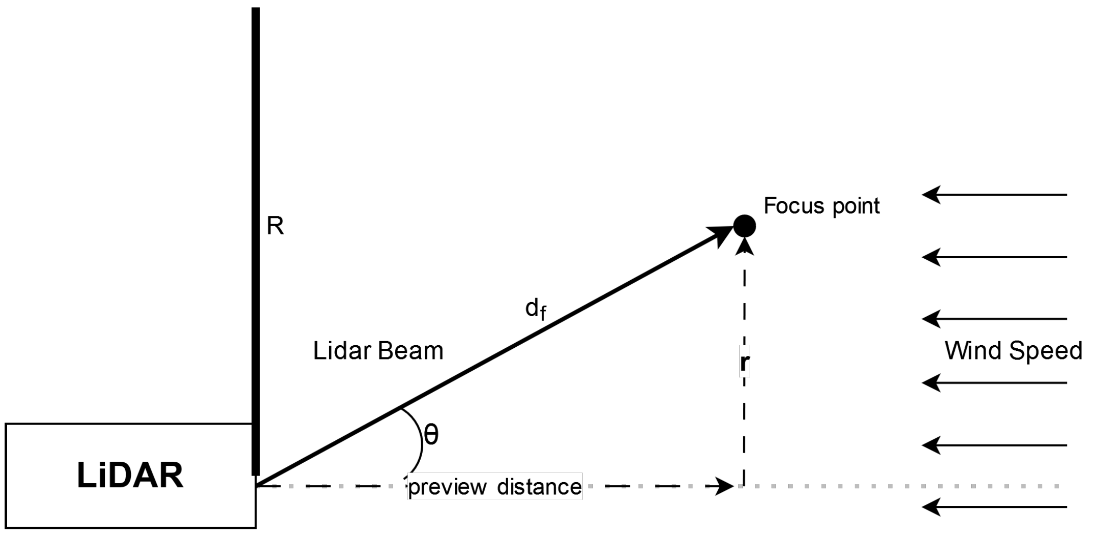
The LiDAR opening angle can be translated into a percentage of the rotor radius covered by the circular measurement pattern, As illustrated in
Figure 2, the focus distance,
, is fixed and
r represents the radius of the circular pattern. This percentage is computed as follows:
where
R denotes the rotor radius. Furthermore, when the half-cone (opening) angle
is changed while keeping the focus distance constant, the preview distance is also affected accordingly.
3.1. Impact on Coherent Wavenumber Under Different LiDAR Configurations and Wind Conditions
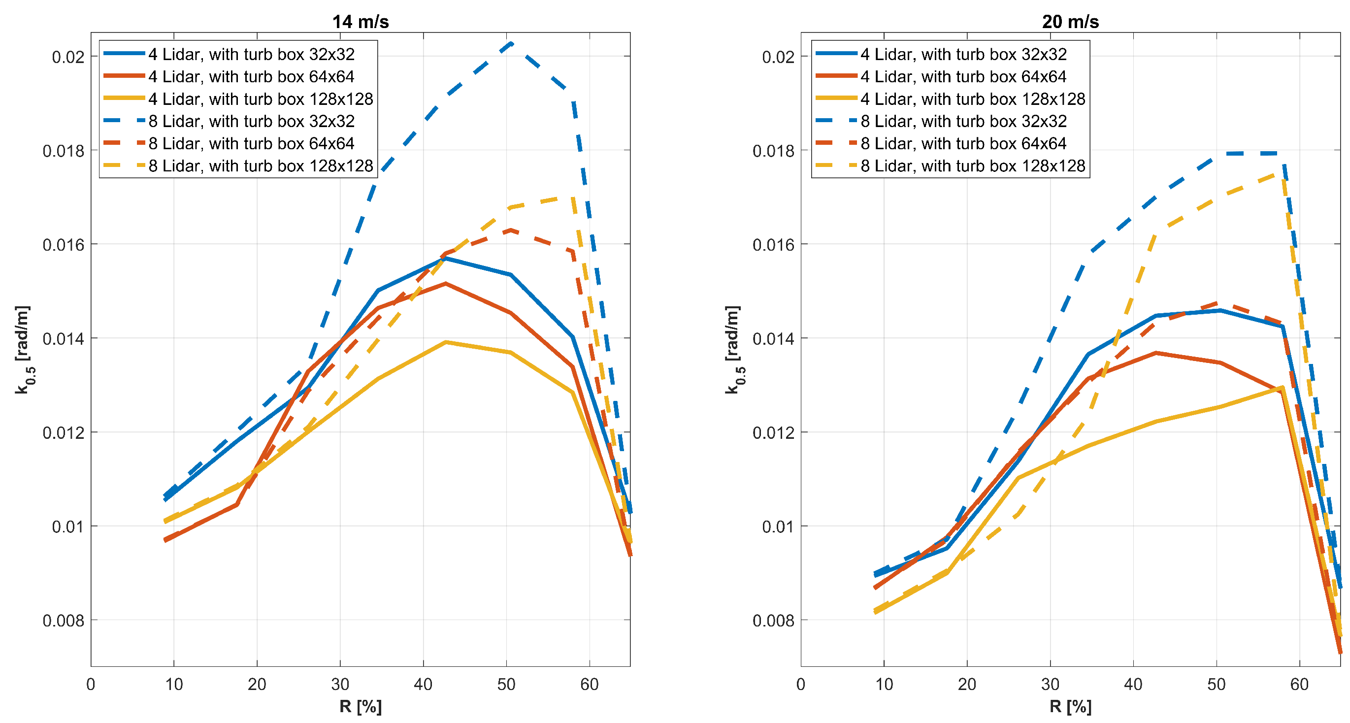
The coherent wavenumber,
, was calculated for each seed and averaged, as shown in
Figure 3 for the configurations with 4 and 8 LiDAR beams, varying the turbulence grid box and half-cone angle. As the resolution of the turbulence box increases, the coherent wavenumber generally decreases. This trend is consistent for both wind speeds of 14 m/s and 20 m/s, and for both LiDAR configurations. Additionally, as the wind speed increases, the coherence wavenumber shows a similar decrease. However, an increase in the number of LiDAR beams leads to an upward trend in coherence, as more beams capture additional details of the rotor area, providing a more accurate representation of the incoming wind speed and improving rotor-equivalent wind speed (REWS) approximations.
Furthermore, as the cone angle increases (with the focus length unchanged, see
Figure 2), expanding the LiDAR coverage over the rotor radius, the coherence increases until it reaches peak points between 50% and 60% of the rotor radius. Beyond this, coherence decreases sharply. This behaviour holds for all simulated cases. The study suggests that for large wind turbines, the best correlation occurs when measurements are taken above 50% of the rotor radius, further supporting the coherence trends observed in this study. These results highlight the complex interplay between turbulence accuracy, wind speed, and the number of LiDAR beams on the coherent wavenumber.
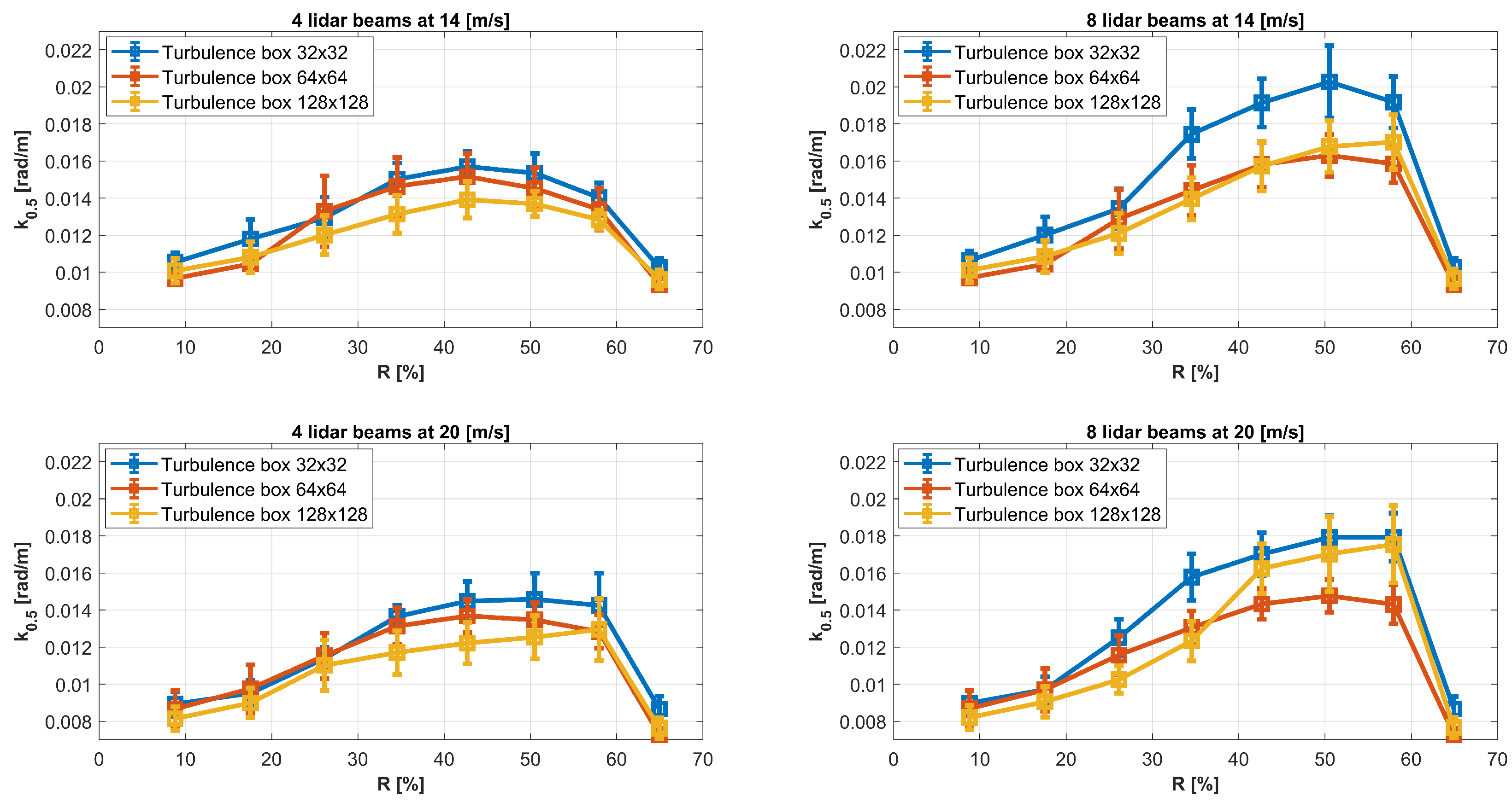
3.2. Uncertainty in Coherence Under Different Realisations of Turbulent Fields
Next, the standard deviation is calculated for each case and presented as error bars, as shown in
Figure 4. The findings of this study indicate that increasing the preview distance (by modifying the half-cone angle) of the LiDAR system leads to a significant rise in the standard deviation, reflecting a greater dispersion of data points around the mean. This effect is most pronounced within the range of 30% to 60% of the rotor radius, where the coherent wavenumber reaches its highest values. This range is particularly significant for simulations, as it is both operationally important and captivating.
Additionally, the data analysis revealed an interesting trend for shorter preview distances, specifically between 10% and 25% of the rotor radius, where greater dispersion of the coherent wavenumber was observed at lower wind speeds. As wind speed increased, the dispersion shifted towards larger preview distances, between 40% and 60% of the rotor radius. It was also noted that the turbulence box with dimensions 32 × 32 (height and width) exhibited higher deviations, likely due to fewer grid points providing less detailed information. Conversely, the turbulence box of 128 × 128 displayed less dispersion for shorter preview distances (10% to 40% of the rotor radius), while the 64 × 64 turbulence box showed less dispersion throughout simulations in the 40–60% range. This behaviour may explain the variations in coherence observed in
Figure 3, as values between 40% and 60% of the rotor radius exhibit higher fluctuations. These factors should be considered when applying the coherent wavenumber and parameters to the filter to ensure an acceptable signal quality for predicting wind speed.
3.3. Summary of Coherence Study
The analysis reveals key insights regarding the turbulence box size, number of LiDAR beams, and opening angle in LiDAR configurations.
Turbulence Box: Increasing the size of the turbulence box from 32 × 32 to 128 × 128 decreases the coherence wavenumber, suggesting that higher-resolution turbulence boxes might result in worse correlation due to higher fidelity simulations. The 64 × 64 turbulence box generally presents lower dispersion across different simulation seeds. It was observed that lower-resolution turbulence boxes (32 × 32) had higher variations and a larger standard deviation in the critical region, while 64 × 64 and 128 × 128 turbulence boxes were more consistent.
Number of LiDAR Beams: Increasing the number of LiDAR beams leads to an increase in the coherence wavenumber, benefiting LiDAR-assisted control by capturing more information. However, further investigation is needed to determine how much the coherence can improve with additional LiDAR beams.
Preview Distance: The coherence wavenumber increases with the preview distance up to 60% of the rotor radius, after which it decreases drastically. This highlights the importance of selecting the optimal preview distance to obtain the best signal quality and coherence. It is also noted that higher windspeeds lead to greater dispersion in coherence, underlining the significance of pre-evaluating parameters for optimal performance.
Based on the observations, the subsequent simulations will utilise a 64 × 64 turbulence box, offering a balance between accuracy and computational efficiency. While a 128 × 128 turbulence box would ideally provide higher resolution, its computational demands are substantial. Therefore, more powerful hardware should be considered before conducting such large-scale simulations.
4. Results: Study of Two Reference LiDAR-Assisted Methods
4.1. Simulation Set-Up
In this simulation study, the IEA 10MW reference wind turbine [
24] with a rotor diameter of 198 m and, the NREL 5MW reference wind turbine [
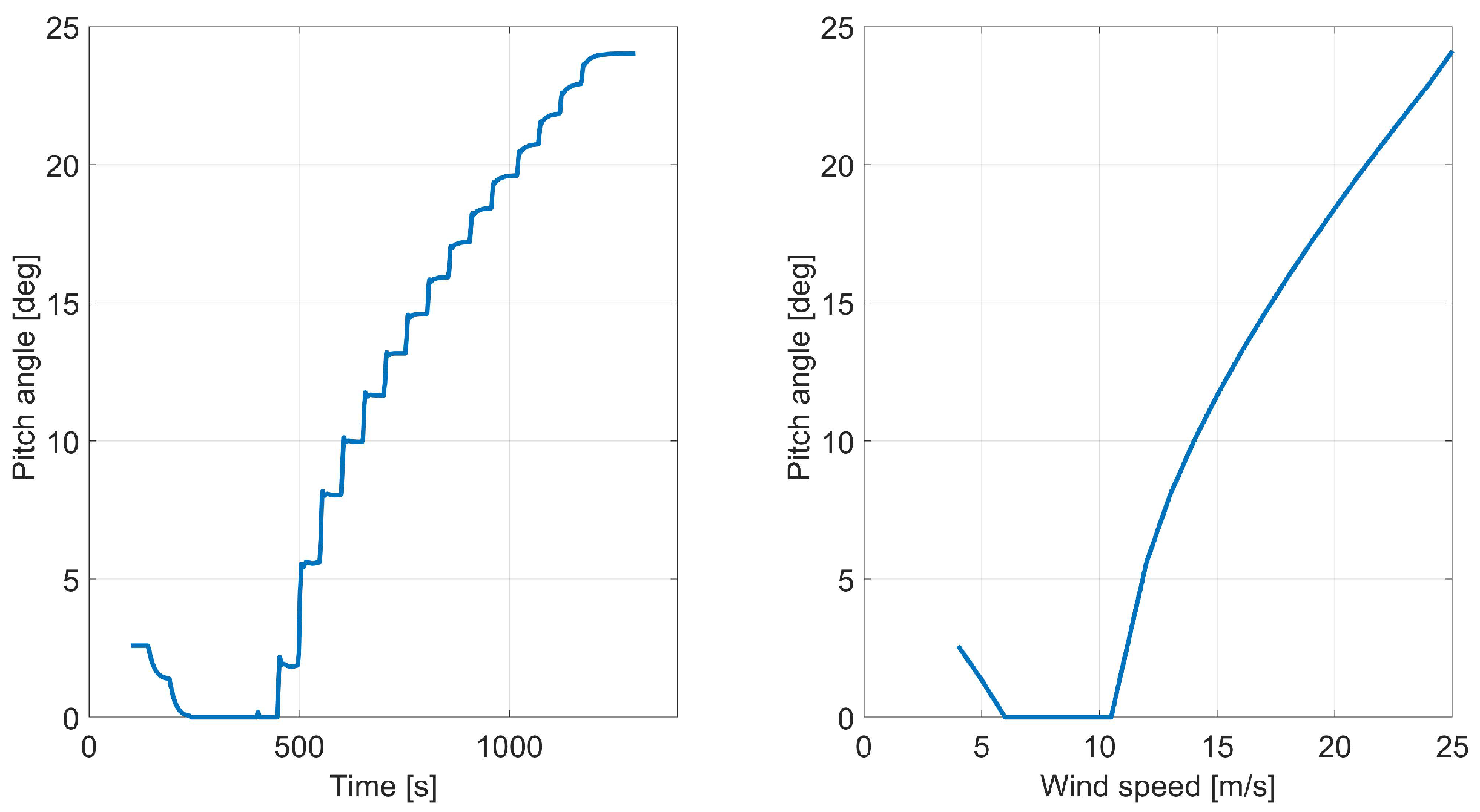
25] with a rotor diameter of 126 m, were used. The baseline setup of a turbulent wind box consists of a grid of 64 × 64 in the plane perpendicular to the flow direction using 8 LiDAR beams in a circular pattern with a minimum half-cone angle that covers 50% of the rotor radius. The preview distance results in 86.6 m. For Schlipf and Bossanyi approaches, the feedforward output pitch angle is extracted based on a steady-state pitch curve derived from HAWC2 steady-state simulations. An example of the steady-state pitch curve for the IEA 10MW reference wind turbine is shown in
Figure 5.
Lastly, to evaluate the two approaches, short-term damage equivalent loads (DELs) averaged among different seeds based on the simulation time series are computed.
4.2. LiDAR-Assisted Control Coherence and Look-Ahead Time
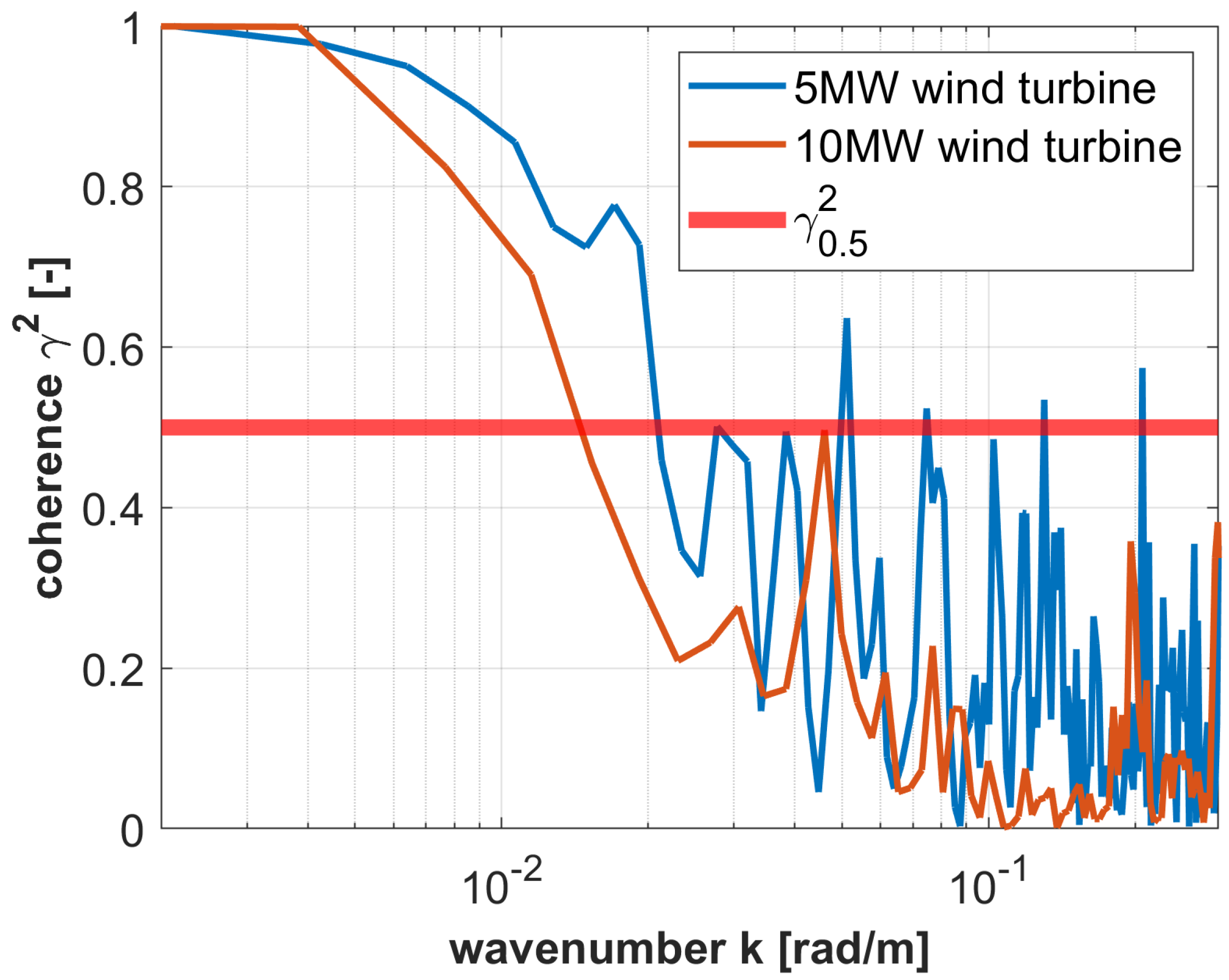
Numerical simulations first showed the results of the coherence difference for the two wind turbines for a mean wind speed of 18 m/s. An example is exhibited in
Figure 6. The coherence study considers six time series for each turbine. The coherent wavenumbers
and
for the IEA 10 MW and NREL 5 MW reference wind turbines respectively were found and utilized.
The look-ahead time
T can be computed using Equation (
2), while the time delay introduced by the Butterworth filter can be approximated from K. Manal and W. Rose [
26], and using the corresponding coherent.
When initially evaluating the case of the IEA 10 MW reference wind turbine, simulations revealed that the selected configuration resulted in the following:
This led to a preview time
T of −0.25 s, which is clearly not feasible, as it suggests that the measured wind speed has already passed the wind turbine.
Upon further examination of the implementation, Equation (
2) is divided into two main components. The first term depends on the LiDAR and the measurement distance (
, where
is the line-of-sight wind speed and
is the half-cone angle). The second term is related to the LiDAR through the filter cut-off frequency. A smaller coherence bandwidth results in a larger
, as indicated by Equation (
12).
In the current results, the magnitude of the second term exceeds that of the first. This is due to the low cut-off frequency, which introduces a significant time delay in the filter. The delay is primarily a consequence of the low coherence bandwidth, , resulting from the limited number of LiDAR beams used in the current configuration.
The simplest solution to address the current issue is to increase the measurement distance X of the LiDAR system, thereby extending the look-ahead time and reducing the impact of the filter delay. However, practical considerations, such as the availability and accessibility of a customised LiDAR system, must also be taken into account.
4.3. Feedforward Method Analysis and Comparison
Results for the feedforward methods are presented in this section, based on (i) the recommended gain adjustments, and (ii) additional fine-tuning aimed at improving performance. The effectiveness of each method is evaluated through a comparison of Power Spectral Density (PSD) of key turbine signals and short-term Damage Equivalent Loads (DELs).
4.3.1. Results with Recommended Controller Tuning
When using the feedforward controllers, the gain adjustment of the feedback controller was performed, where the reduction in the integral gain (
) should be, in general, the square of the reduction in the proportional gain (
) [
20]. For the Schlipf approach, adjustments are carried out as per the author’s recommendation to halve the proportional gain of the feedback controller [
20]. Bossanyi’s approach followed the findings in Meng et al. [
4], optimizing the gains to 90% of the original feedback signal [
4].
Simulations were carried out for LiDAR-assisted control using both feedforward approaches on the NREL 5MW reference wind turbine. For comparison, the baseline controller used was the DTU open-source PI feedback controller. The simulations were performed under turbulent wind conditions at a mean wind speed of 18 m/s. The selected LiDAR configuration resulted in a preview time,
T, of 1s. The results are shown in
Figure 7a,b, which illustrate an example of the LiDAR-measured wind speed compared with the rotor effective wind speed (REWS), as well as the corresponding pitch angle response for the chosen coherence.
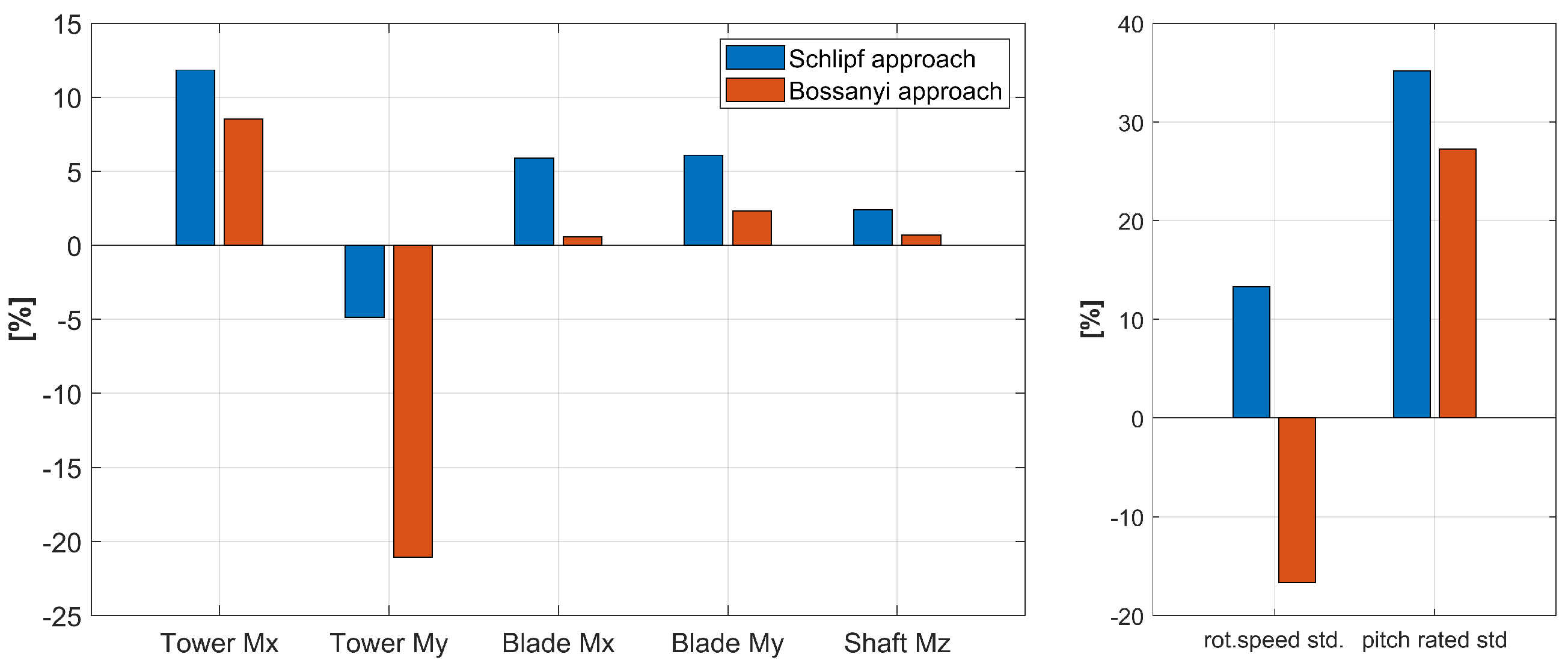
To evaluate the approaches in terms of load reduction, short-term DELs were computed.
Figure 8 shows the difference between the baseline and the studied methods, where a positive magnitude represents a load reduction.
It is first revealed a decrease in the tower bottom fore-aft loads. This reduction is due to the diminished influence of wind disturbances on the rotor speed at lower frequencies, facilitated by the LiDAR. However, it is also noticed a clear increase in the tower bottom side-to-side loads particularly employing the Bossanyi approach. Minor load reductions are also appreciated on the blade loads.
To gain further insights into the increase in the tower load, the PSD of the pitch angle and tower side-to-side were computed (see
Figure 7c,d). It is clearly visible a notable peak at the first tower side-to-side natural frequency (0.32 Hz) in both the baseline and the feedforward methods, mainly in the Bossanyi approach. This is due to the fact that the Bossanyi approach incorporates the actual pitch angle, allowing any baseline controller-induced frequencies to propagate into the feedforward design, as evidenced by the collective pitch angle PSD. As a result, this excitation is also noticeable in the PSD of the tower side-to-side moment, as illustrated in
Figure 7d. The increased power spectral density at the first tower’s side-to-side natural frequency contributes to the increased loads experienced by the tower.
Furthermore, a frequency transport phenomenon is observed when using the Bossanyi approach, arising from both the use of the current pitch angle to calculate the feedforward pitch rate and the design implementation. In Bossanyi’s approach (Equation (
10)), the actual pitch angle (
) contains components at the tower frequency, which are then fed back into the integrator through the feedforward design. As a result, Bossanyi’s approach imposes a higher requirement on the quality of the feedback design, demanding that the closed-loop system exhibits a low-frequency response at the tower frequency. This, in turn, influences the excited frequencies and ultimately impacts the Damage Equivalent Loads (DELs) in the tower side-to-side direction.
4.3.2. Results with Controller Fine-Tuning
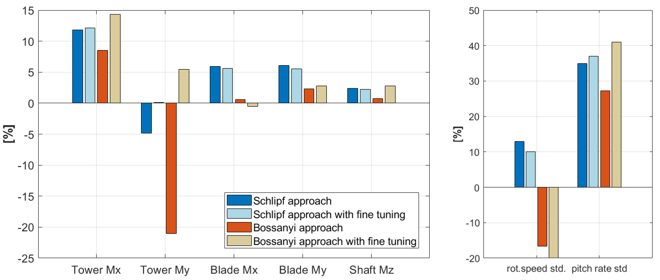
Building on the previous findings, simulations were repeated in a scenario aimed at minimising the tower’s side-to-side moment. The controller was fine-tuned by reducing the frequency of the generator speed filter in the feedback loop from 0.4 Hz to 0.25 Hz. The results for the short-term DELs, alongside the previous DELs results, are presented in
Figure 9.
In this case, it is evident that the Schlipf approach achieves comparable load reduction in both scenarios, despite a 4% increase in the short-term tower side-to-side DELs. This increase is attributed to changes in the feedback loop filtering, specifically a reduction in the control bandwidth well below the tower frequency. As expected, this indicates that the Schlipf approach performs more robustly in low-frequency regulation, even when tower frequency components are present in the feedback controller.
Opposing this, the Bossanyi approach seems to be more sensitive to the performance of the baseline feedback controller. When the interaction with the tower side-to-side frequency is diminished in the feedback control design, Bossanyi’s approach has the potential to improve load reduction on tower bottom side-to-side moment.
5. Conclusions
This study initially focused on the effective use of wind measurements from commercially available LiDAR systems, evaluating how LiDAR configuration such as the number of beams, locations of the beams, and turbulence box resolution in HAWC2 simulations affects signal coherence. Results showed that improving the turbulence box resolution leads to lower coherent wavenumbers, while low-resolution boxes introduce greater variability across seeds. Overall, grids of 64 × 64 and 128 × 128 performed similarly, although the grid of 128 × 128 showed less dispersion for short preview distances. Increasing the number of LiDAR beams improved coherence, particularly when measurements were taken between 40–60% of the rotor radius; coherence dropped significantly outside this range. Wind speed increases were found to reduce coherence, suggesting a need for adaptive filters. Overall, for more accurate aeroelastic simulations, at least eight LiDAR beams should be used, with measurements taken at a minimum of 40% rotor radius, and a turbulence box grid of at least 64 × 64.
Next, the simulation results of the presented work initially revealed that larger wind turbines exhibit reduced coherence bandwidth when using the same LiDAR system compared to smaller sizes. Additionally, challenges were identified in correcting the time required to compensate for the filter time delay,
. It was found that in larger wind turbines, such as the IEA 10MW reference wind turbine, the time needed to compensate for the time delay caused by the filter can exceed the available preview time from Equation (
2). This phenomenon arises from the limited coherence bandwidth associated with the available LiDAR beams. As a consequence, the Butterworth filter exhibits a low cut-off frequency, leading to an increased value of
.
These results underscore the critical importance of ensuring a sufficiently high coherence to effectively compensate for the time delay without compromising the available preview time due to the interplay between the measurement, coherence, and cut-off frequency of the filter. The specific threshold of coherence may vary depending on the particular setup and wind turbine size to guarantee a successful implementation when using LiDAR measurements. Addressing this issue may involve optimizing measurements to increase coherence bandwidth or increasing the preview time through the measurement distance. Notably, this phenomenon is not evident in simulations for smaller wind turbines, such as the NREL 5 MW reference wind turbine.
In the assessment of short-term DELs reduction, the Schlipf approach demonstrated overall better performance compared to the Bossanyi approach where deficiencies were observed including frequency propagation and higher excitation in existing natural frequency of the tower, as illustrated in
Figure 7c,d. These issues resulted from utilizing the actual pitch angle for feedforward pitch rate calculation that might contains signal component at the tower frequency. Despite these challenges, fine-tuning of the the feedback controller allowed the Bossanyi approach to yield positive outcomes and outperform the Schlipf approach in terms of load reduction on tower side-to-side moment, as shown in
Figure 9. In contrast, the Schlipf method demonstrated robustness and achieved its two primary objectives—reference signal tracking and disturbance compensation. Overall, the Schlipf approach exhibited a more robust and reliable performance in load reduction, regardless of the feedback controller design.
These insights point to several implications for future turbine control design. First, there is a clear need to co-design LiDAR systems and control algorithms to ensure sufficient coherence and preview quality. Second, the development of adaptive filtering techniques and improved scanning strategies could help mitigate coherence loss in large turbines. Finally, controller robustness must be a design priority to ensure safe and effective integration of feedforward control, particularly as rotor diameters and structural flexibility continue to increase in next-generation turbine designs.
In the future, this study will be extended to include a full design load case analysis. In the current work, the comparison of the two feedforward methods was limited to a wind speed of 18 m/s due to time constraints. This speed was selected as it represents above-rated conditions where pitch control is dominant. Six turbulence seeds were used to capture variability and provide averaged results. While only one wind speed was considered, we expect the relative trends in load impact between the two methods to remain consistent across other above-rated wind speeds.
Further work will also explore filtering strategies, such as applying a notch filter at the tower frequency to remove tower-induced components from the LiDAR signal. In addition, the study will investigate and optimise alternative LiDAR measurement patterns and configurations for larger wind turbines. The circular scan pattern used here serves as a baseline, and future efforts will explore new patterns and combinations with varying focal distances to improve the accuracy and effectiveness of LiDAR-assisted control.


