A Comparative Evaluation of Harmonic Analysis and Neural Networks for Sea Level Prediction in the Northern South China Sea

Abstract

Long-term sea level variations in the northern South China Sea (SCS) are known to significantly impact coastal ecosystems and socio-economic activities. To improve sea level prediction accuracy, four models—harmonic analysis and three artificial neural networks (ANNs), namely genetic algorithm-optimized back propagation (GA-BP), radial basis function (RBF), and long short-term memory (LSTM)—are developed and compared using 52 years of observational data (1960–2004). Key evaluation metrics are presented to demonstrate the models’ effectiveness: for harmonic analysis, the root mean square error (RMSE) is reported as 14.73, the mean absolute error (MAE) is 12.61, the mean bias error (MBE) is 0.0, and the coefficient of determination (R²) is 0.84; for GA-BP, the RMSE is measured as 29.1371, the MAE is 24.9411, the MBE is 5.6809, and the R² is 0.4003; for the RBF neural network, the RMSE is calculated as 27.1433, the MAE is 22.7533, the MBE is 2.1322, and the R² is 0.4690; for LSTM, the RMSE is determined as 23.7929, the MAE is 19.7899, the MBE is 1.3700, and the R² is 0.5872. The key findings include the following: (1) A significant sea level rise trend at 1.4 mm/year is observed in the northern SCS. (2) Harmonic analysis is shown to outperform all ANN models in both accuracy and robustness, with sea level variations effectively characterized by four principal and six secondary tidal constituents. (3) Despite their complexity, ANN models (including LSTM) are found to fail in surpassing the predictive capability of the traditional harmonic method. These results highlight the continued effectiveness of harmonic analysis for long-term sea level forecasting, offering critical insights for coastal hazard mitigation and sustainable development planning.

1. Introduction

1.1. Research Background

Coastal regions are the epicenters of global human habitation and economic activity. Approximately 80% of the world’s population resides in these areas, and in China, about 70% of major cities are located along the eastern coast. These coastal zones, with their economic prosperity and high population density, are crucial for national economies. However, they are highly vulnerable to sea level changes. Sea level fluctuations can severely disrupt the entire ecosystem and human life [1,2,3]. Over the past century, the study of sea level change has become one of the most closely watched scientific issues. For example, Khan et al. (2024, 2025) emphasized the significance of sea level rise in predicting long-term coastal line changes [4,5]. The northern South China Sea, situated at the transitional zone between the southern edge of mainland China and the South China Sea, has a unique climate. It is mainly influenced by the East Asian monsoon and is also affected by El Niño–Southern Oscillation (ENSO) events [6] and typhoons [7]. As a result, it is a sensitive area for sea level variations. Under the backdrop of global warming, sea level changes in the northern South China Sea have significant impacts on the local ecological environment and socio-economic development. In recent years, the sea level in the South China Sea has attracted increasing attention. Over the past 40 years, the sea level in this region has been rising at an average rate of around 3.5 mm/a. Satellite altimetry data show that since 1993, the sea level has been rising at a more significant rate of approximately 4 mm/a [8].

1.2. Current Research Status

Research on sea level change has been carried out on a global and regional scale. In terms of global research, it is well known that sea level changes are driven by multiple factors, such as glacier and ice sheet melt, thermal expansion of seawater, and terrestrial water storage variations. Regionally, Mohamed and Skliris investigated sea level changes in the Red Sea over the 29-year period from 1993 to 2021. By analyzing the long-term trend and interannual variations in total sea level anomaly (SLA), they found that the total SLA and spatial SLA trend in the northern Red Sea (NRS) are higher than those in the southern Red Sea (SRS), which is influenced by the low-salinity upwelling from the Gulf of Aden [9]. Meli et al. reconstructed a refined local geocentric sea level time series for the coastal plain of Emilia-Romagna in northern Italy from 1993 to 2020. They processed data from tide gauges and satellite altimetry and observed a relative sea level rise across the entire region. Due to local subsidence related to subsurface fluid extraction, the relative sea level rise exceeded the geocentric rise by 55% to 640%, and critical points were identified, leading to severe flood risks [10]. Xiao et al. proposed a continuous piecewise polynomial fitting algorithm to detect breakpoints in sea level records. Their study revealed that the global mean sea level rise driven by glacier mass loss shifted from a linear increase to an accelerated trend around 1962 ± 1, with two dominant periodic signals of about 52 and 27 years [11]. Zhang et al. [12] conducted high-resolution detrital mineral analysis on sediments from a 70.20-m borehole (Core CRE-1402) in the Yangtze Shoal. The results indicated that sea level rise leads to river channel incision, estuary southward migration, and sediment redistribution. During high sea level periods, the Yangtze River estuary migrates southward, resulting in sediment starvation in this region. In contrast, during sea level rise phases, the Yangtze River channel may shift and supply sediments to the Yangtze Shoal [12].

There are several methods for studying sea level change. Tide gauge observations [13] have long been used to measure relative sea level change at specific coastal points. Satellite altimetry [14] is a powerful technique for measuring absolute sea level change over a vast ocean surface. It uses radar or laser altimeters on satellites to measure the distance from the satellite to the sea surface, enabling the creation of accurate maps of ocean surface topography. Gravity satellite missions [15] can monitor changes in terrestrial water storage, which is one of the factors affecting sea level. Geological and paleoclimate proxies [16] help reconstruct past sea level changes. GPS and crustal motion monitoring [13] are used to account for land movement, which is important for accurately understanding relative sea level change. Numerical modeling [17] can simulate sea level change under different scenarios, and synthetic aperture radar interferometry (InSAR) [18] can provide high-resolution measurements of land surface deformation related to sea level change.

In terms of sea level prediction, current research hotspots focus on the driving mechanism of sea level variations [19,20,21,22,23] and the prediction model of sea level change [24,25,26,27,28]. Commonly used methods for sea level prediction include global climate models, regional downscaling techniques, and semi-empirical models. Sun et al. (2020) [29] proposed a combined SARIMA and LSTM prediction model. The SARIMA model was used to predict the trend and seasonal components of sea level change, while the LSTM model predicted the random component. The results showed that the proposed model had good prediction performance, with a minimum root mean square error of 1.155 cm and a maximum coefficient of determination of 0.89. Zhao et al. (2019) [25] analyzed sea level changes around the Shandong Peninsula from 1993 to 2016 using the fully integrated empirical mode decomposition (CEEMD) method and a radial basis function (RBF) network based on satellite altimetry gridded sea level anomaly (SLA) data. The results indicated that CEEMD was suitable for analyzing nonlinear and non-stationary time series, and RBF networks were suitable for predicting regional sea levels at different scales. Hyun et al. (2016) [30] investigated the influence of atmospheric pressure changes on sea level prediction along the eastern coast of South Korea. They applied the inverted barometer effect (IBE) to the Telemac-2D model for simulation and analysis. The findings showed that the predictive correlation of IBE combined with tides was better than that of tides alone, and they recommended using the IBE in numerical simulations of sea level changes in the East Sea.

1.3. The Research Contents of This Study

However, research on predicting sea level changes in the northern South China Sea is currently limited. The northern South China Sea is affected by complex climate systems such as the East Asian monsoon, ENSO events, and typhoons. The interactions among these factors result in highly variable and nonlinear sea level changes, which pose challenges to the traditional linear assumptions and fixed-parameter settings of common prediction models. Moreover, the data related to sea level changes in this region often have issues such as data gaps, noise interference, and inconsistent spatiotemporal resolutions. Many common prediction methods lack effective strategies to handle these complex data situations, leading to potential inaccuracies in prediction results. The central question of this study is how to effectively predict sea level changes in the northern South China Sea, considering its complex climate-driven dynamics and data-related challenges. Specifically, can harmonic analysis and advanced machine learning models (GA-BP neural network, RBF neural network, and LSTM neural network) better capture the characteristics of sea level variations in this region compared to existing methods? We developed four prediction models, namely harmonic analysis, the GA-BP neural network, the RBF neural network, and the LSTM neural network, using long-term tide gauge data from the northern South China Sea. We evaluated and compared the performance of these four models in handling the nonlinearity, high-dimensionality, and temporal complexity of sea level variations in the northern South China Sea. We determined the most suitable model for predicting sea level changes in the northern South China Sea, providing a scientific basis for disaster prevention, mitigation, and the sustainable development of the region.

1.4. The Contributions of This Study

This study contributes to existing research in several ways. First, it targets the northern South China Sea—a climatically sensitive transition zone between mainland China and the South China Sea, where approximately 70% of China’s major cities are concentrated. Despite its economic significance and high vulnerability to sea level changes (driven by East Asian monsoons, typhoons, and ENSO events), this region has remained understudied in sea level prediction research. So, this study fills the gap in existing regional research. Second, while harmonic analysis (a well-established method for periodic signal processing [31,32]) and machine learning models (e.g., RBF, LSTM) have been individually used in sea level research, this study innovates by conducting the first comprehensive comparative evaluation of four methodologies—harmonic analysis, GA-BP, RBF, and LSTM—within a unified framework for the northern South China Sea. The GA-BP neural network, with genetic algorithms (GAs) optimizing the weights of the backpropagation (BP) network, can better avoid local minima and improve prediction accuracy in complex nonlinear systems. The RBF neural network, with its strong local approximation ability and fast convergence speed, is suitable for handling high-dimensional and non-stationary sea level data. The LSTM neural network, as a variant of recurrent neural networks, can capture long-term temporal dependencies in sequential data, which is crucial for modeling the long-term trends and periodic fluctuations in sea level changes [33]. Unlike prior single-model studies, this study evaluates how each model handles the region’s high-dimensional, non-stationary data and data gaps, providing a practical framework for evidence-based model selection in real-world coastal management. Thirdly, by leveraging long-term tide gauge data, this study further tests model robustness against the northern South China Sea’s specific data challenges, bridging the gap between theoretical modeling and regional disaster mitigation needs.

2. Data and Methods

2.1. Data

The sea level data in this paper are obtained from the Zhapo Marine Station in Jiangcheng District, Yangjiang City, Guangdong Province (Figure 1). The Zhapo Marine Station is located in the northern part of the South China Sea and was established in 1957. It is recognized as one of the earliest tide gauge stations in China. The sea level data provided by this station are considered highly reliable for the northern South China Sea region. The sea surface data presented in this paper cover the period from 1970 to 2021, and they represent the longest instrumental record of sea level variations currently available in the northern South China Sea. 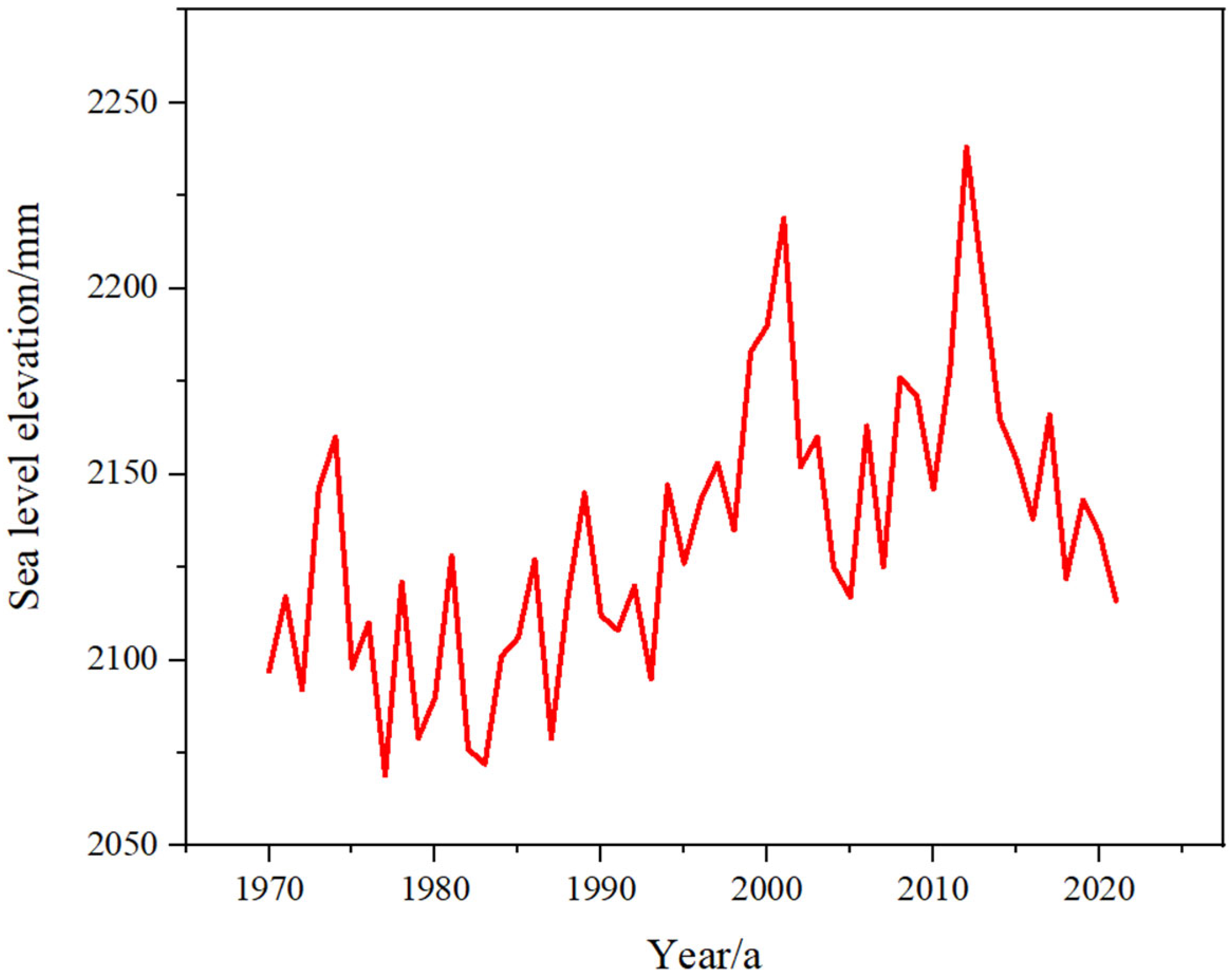As we can see from Figure 2, the maximum sea level in the northern South China Sea over the past 52 years is 2238 mm, the minimum is 2069 mm, the average is 2134 mm, and the range (the difference between the maximum and minimum values) is 169 mm. From Figure 2, it can be seen that the sea level in the northern South China Sea exhibits three characteristics, as follows:

(1)

Trend. The sea level in the northern South China Sea shows a clear upward trend.

(2)

Fluctuation. A series of interannual and interdecadal fluctuations are superimposed on the upward trend of sea level, which indicates the periodicity of sea level changes.

(3)

Instability. The sea level fluctuations are unstable. There are particularly small fluctuations in certain periods such as 1979–1998, as well as particularly intense fluctuations in other periods such as 2000–2014.

Figure 1. Schematic diagram of location of Zhapo Marine Station (marked by red five-pointed star).

Figure 1. Schematic diagram of location of Zhapo Marine Station (marked by red five-pointed star).

Figure 2. Sea level variation of northern South China Sea from 1970 to 2021.

Figure 2. Sea level variation of northern South China Sea from 1970 to 2021.

2.2. Harmonic Analysis

Harmonic analysis is a time-series analysis method; its core idea is to regard a complex time series as the result of the superposition of many harmonic vibrations with different frequencies. Mathematically, the Discrete Fourier Transform involves expressing a complex periodic function as a series of simple trigonometric functions, as shown in Equation (1).

$$\mathrm{f}\left(\mathrm{t}\right)={\mathrm{A}}_0+{\sum }_{\mathrm{n}=1}^{\mathrm{\infty }}{\mathrm{A}}_{\mathrm{n}}\sin (\mathrm{n}\omega \mathrm{t}+{\phi }_{\mathrm{n}})$$

(1)

where A0, An, and φn are all constants.

Harmonic analysis can extract periodic signals in a time series, helping us to understand the causes of time-series fluctuations and further analyze the driving mechanisms of the time series. Usually, only the most prominent few peaks are analyzed when selecting harmonics, and other harmonics are regarded as random phenomena. The goodness of fit can be judged based on the variance in each harmonic. Prediction can be achieved by extending the time series based on harmonic analysis.

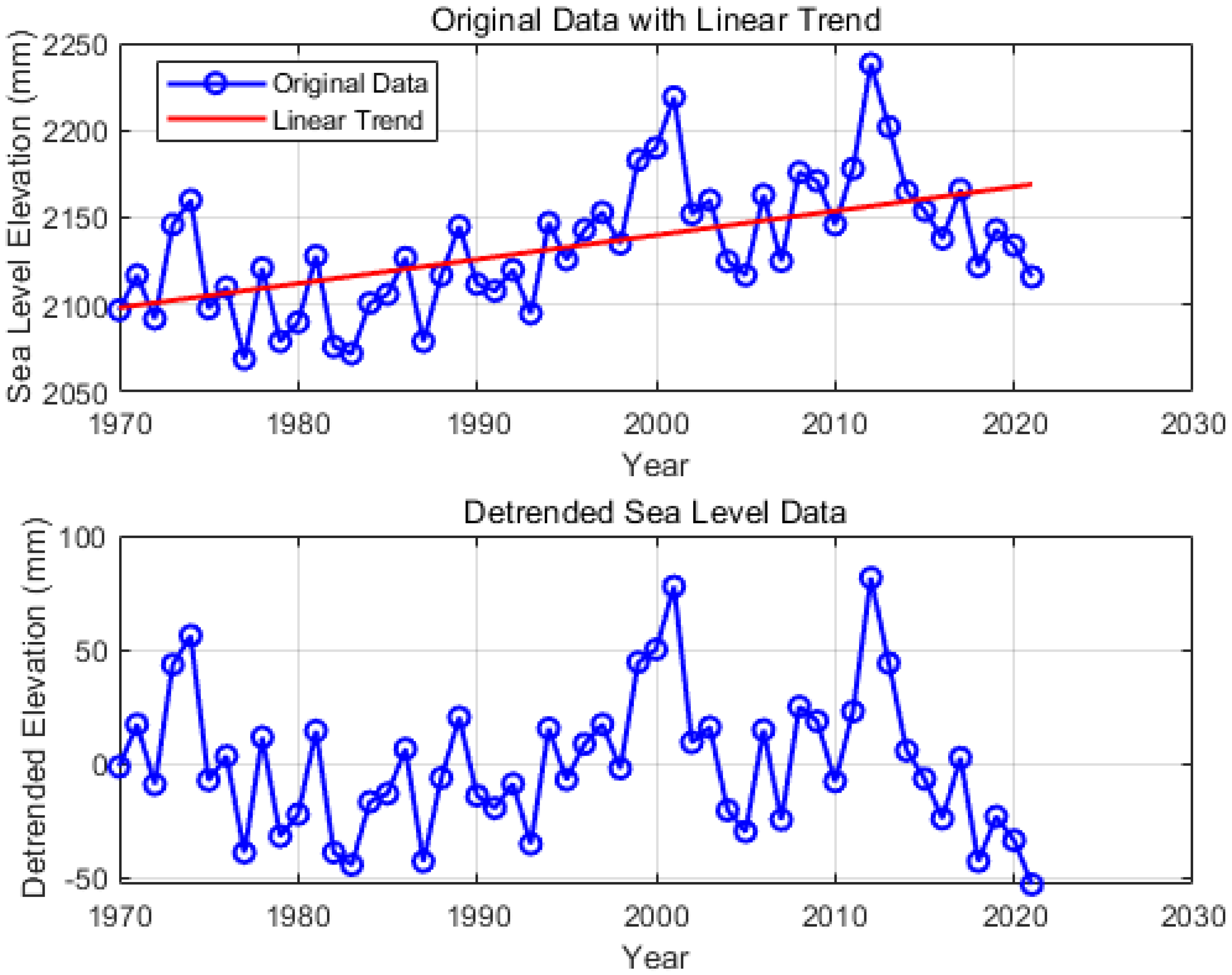
The raw sea level data (1970–2021) contain long-term trend components and periodic fluctuations. In this study, a linear fitting method is used for detrending, with the specific steps as follows:

(1)

Trend component extraction: Linear regression is performed on the raw data using the least squares method to obtain the trend equation

$${\mathrm{y}}_{\mathrm{z}\mathrm{p}}=1.3852\times \mathrm{t}-630.5003,$$

where $\mathrm{t}$ is the year and ${\mathrm{y}}_{\mathrm{z}\mathrm{p}}$ is the sea level height of the trend component, which explains approximately 78% of the long-term trend variation in the data (${\mathrm{R}}^2=0.78$).

(2)

Residual series generation: The raw data are subtracted by the trend component to generate the detrended residual series ${\mathrm{y}}_{\mathrm{d}\mathrm{p}\mathrm{r}}$, which contains only periodic fluctuation components for subsequent harmonic analysis.

(3)

Data validation: The effectiveness of trend extraction is validated by calculating the standard deviations of the data before and after detrending (28.5 mm for raw data and 18.2 mm for detrended data), indicating that the detrending process successfully separates the aperiodic components.

The sea level time series contains periodic variations of multiple time scales, among which the most obvious and significant for research are seasonal variations and multi-year variations. From the variation curve of sea level, it can be seen that its fluctuations are relatively regular and can be approximately fitted and represented using cosine or sine functions.

$${\mathrm{H}}_{\left(\mathrm{s}\mathrm{l}\right)}=\sin (\omega \mathrm{t}+\phi )$$

(2)

where H(sl) represents sea level height, and t represents time.

In practical calculations, harmonic theory provides objective and accurate formulas for calculating the phase and amplitude, as follows:

$${\mathrm{H}}_{(\mathrm{s}\mathrm{l}-\mathrm{t})}=\overline{{\mathrm{H}}_{\left(\mathrm{s}\mathrm{l}\right)}}+\mathrm{C}\cos ({\displaystyle \frac{2\pi \mathrm{t}}{\mathrm{n}}}-\phi )=\overline{{\mathrm{H}}_{\left(\mathrm{s}\mathrm{l}\right)}}+\mathrm{A}\cos \left({\displaystyle \frac{2\pi \mathrm{t}}{\mathrm{n}}}\right)+\mathrm{B}\left({\displaystyle \frac{2\pi \mathrm{t}}{\mathrm{n}}}\right)$$

(3)

where $\overline{{\mathrm{H}}_{\mathrm{s}\mathrm{l}}}$ represents the annual mean sea level, n represents the data length, and t represents the year.

According to the theory of least squares, the expressions for A and B can be obtained as follows:

$$\mathrm{A}={\displaystyle \frac{2}{\mathrm{n}}}{\sum }_{\mathrm{i}=1}^{\mathrm{n}}{\mathrm{H}}_{(\mathrm{s}\mathrm{l}-\mathrm{t})}\cos ({\displaystyle \frac{2\pi \mathrm{t}}{\mathrm{n}}})$$

(4)

$$\mathrm{B}={\displaystyle \frac{2}{\mathrm{n}}}{\sum }_{\mathrm{i}=1}^{\mathrm{n}}{\mathrm{H}}_{(\mathrm{s}\mathrm{l}-\mathrm{t})}\sin ({\displaystyle \frac{2\pi \mathrm{t}}{\mathrm{n}}})$$

(5)

After obtaining the values of A and B, the phase can be calculated using Equation (6).

$$\varphi =\left\{\begin{array}{cc}\arctan ({\displaystyle \frac{\mathrm{B}}{\mathrm{A}}}),\hfill & \mathrm{A}>0\hfill \\ \arctan \left({\displaystyle \frac{\mathrm{B}}{\mathrm{A}}}\right)\pm \pi ,\hfill & \mathrm{A}<0\hfill \\ {\displaystyle \frac{\pi }{2}},\hfill & \mathrm{A}=0\hfill \end{array}\right.$$

(6)

2.3. GA-BP Neural Network

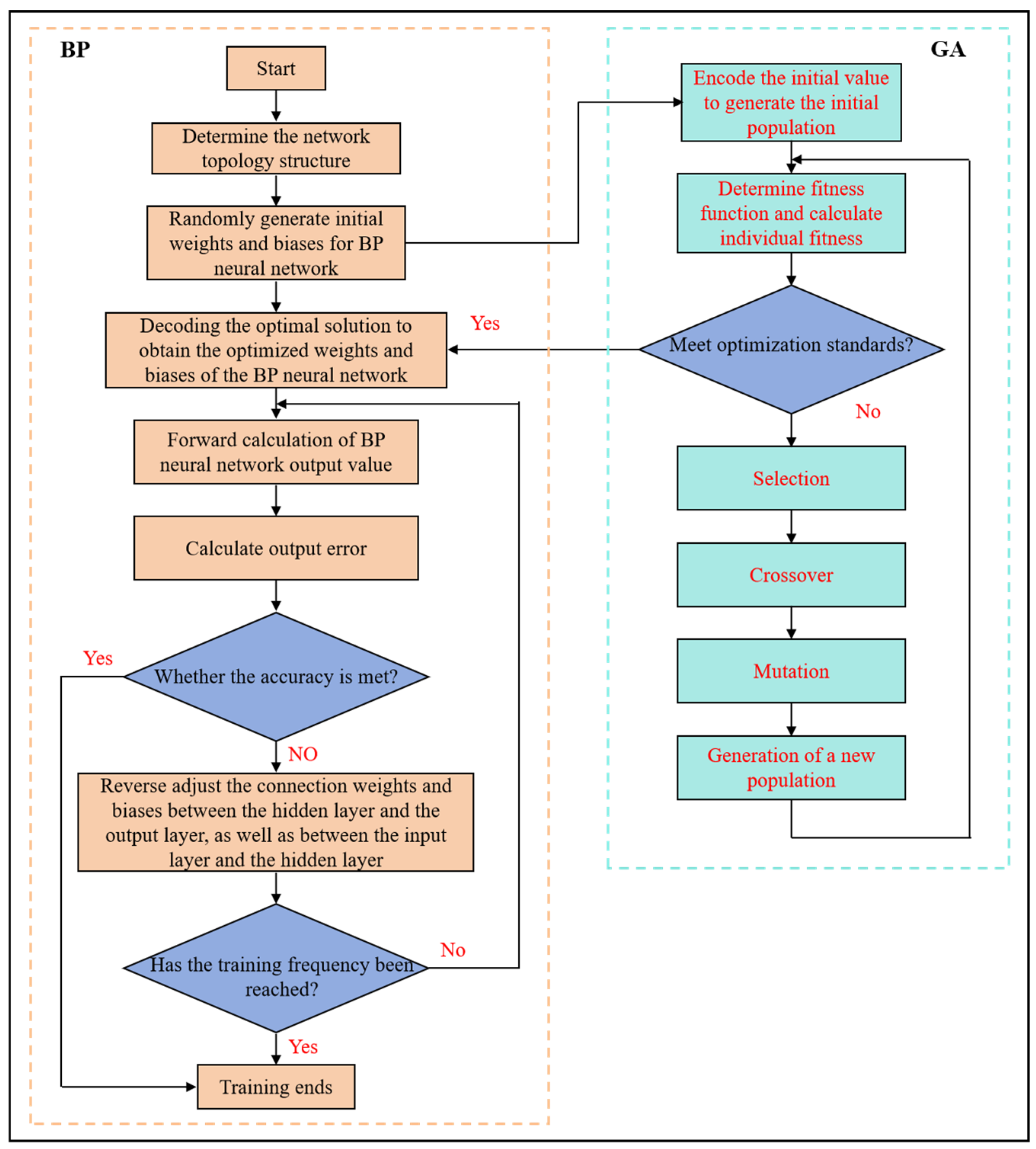
The BP neural network is prone to becoming trapped in local minima when handling nonlinear problems, whereas the global search capability of genetic algorithms (GAs) can optimize initial weights and network structures. In this study, the initial weights and structure of the BP neural network are optimized by GAs to prevent traditional BP neural networks from converging to local minima while improving the model’s convergence speed and generalization ability. Sea level variations in the northern South China Sea are characterized by strong nonlinearity due to complex influencing factors such as monsoons and typhoons. GA-BP is demonstrated to enhance the model’s fitting capability for complex nonlinear relationships by avoiding local optima. The GA-BP neural network is considered particularly suitable for simulating the inherent complex nonlinear relationships in sea level variations of the northern South China Sea. A schematic diagram of the GA-BP neural network is illustrated in Figure 3.

Figure 3 is the original diagram, showing the GA-BP neural network process. The process is divided into the BP neural network section (orange area on the left) and the genetic algorithm (GA) section (blue-green area on the right).

• The BP neural network section:

The process starts from ‘Start’. Firstly, we determine the network topology structure, which determines the basic architecture of the neural network, such as the number of neurons in the input layer, hidden layer, and output layer. We randomly generate the initial weights of the BP neural network, which will be continuously adjusted during subsequent training. Next, we determine whether the genetic algorithm-optimized optimal solution of biases of the BP neural network has been received. If received, we decode it and apply it to the BP neural network; if not received, we proceed to the next step. We perform forward calculations of the BP neural network output value and calculate the output value based on the input data and current weights. We calculate the output error and obtain the error by comparing it with the actual value. If sufficient accuracy has been achieved, the training ends; if the accuracy is not satisfactory, we adjust the connection weights in reverse, including the weights between the output layer and the hidden layer, as well as between the input layer and the hidden layer. Then, we determine if the training frequency has reached the required level. If achieved, the training ends; if not reached, we continue with forward calculations and the other steps.

• The genetic algorithm section:

Firstly, we encode the initial values into genes and generate a population. Then, we transform the initial weights and other parameters of the BP neural network into gene forms that can be processed by genetic algorithms to form the initial population. We determine the fitness function and calculate the fitness value, which is used to evaluate the quality of each individual (i.e., a set of parameters) in the population. We determine whether it meets the optimization standards. If satisfied, we pass the optimal solution to the BP neural network; if not satisfied, we perform a selection operation to select the better individual. We perform a crossover operation to exchange and recombine the genes of the selected individual, resulting in a new individual. We perform mutation operations to make small probability random changes to an individual’s genes, increasing the diversity of the population. We generate a new population, and repeat the fitness calculation, selection, crossover, mutation, and other operations until the optimization criteria are met.

The maximum number of iterations is 1000, the error threshold is ${10}^{-6}$, the learning rate is 0.01, the genetic number is 50, and the population size is 5. The number of iterations and genetic generations are determined through preliminary experiments. In these experiments, when iterations exceed 1000 times, the reduction in model error (RMSE) becomes less than 1%, and continued training tends to cause overfitting. An error threshold of 10⁻⁶ is commonly adopted in machine learning model training to evaluate convergence accuracy. In geophysical prediction fields (such as sea level change), this threshold ensures that the deviation between model predictions and true values remains within the acceptable millimeter range. For the GA-BP model, the maximum number of iterations is set to 1000, combined with the 10⁻⁶ error threshold, effectively preventing underfitting due to insufficient iterations or overfitting caused by excessive iterations. A learning rate of 0.01 represents a classical empirical value in neural network training, suitable for most gradient descent algorithms. This value ensures that parameter updates maintain sufficiently large step sizes (avoiding overly slow convergence) while preventing oscillation or divergence resulting from excessively large steps. The population size is set to 5 because a smaller population reduces computational load, and the crossover/mutation operations in GA already guarantee solution diversity.

2.4. RBF Neural Network

The single-hidden-layer structure and local approximation characteristics of Gaussian functions in RBF neural networks enable their training speed to be significantly accelerated compared with other networks, making them suitable for rapid modeling. In the northern South China Sea where typhoons occur frequently, high-frequency noise is prominently observed in the data. The local learning capability of RBF networks is demonstrated to reduce noise interference, while their single-hidden-layer structure ensures fast training speed, allowing for rapid capture of short-term sea level fluctuations (such as transient changes induced by typhoons). This makes the RBF particularly suitable for real-time prediction scenarios. Additionally, RBF neural networks are characterized by simple structures and minimal parameter adjustment requirements. These features render them highly suitable for predicting sea level variations in the northern South China Sea where available data are limited.

Figure 4 is a diagram of the architecture of the radial basis function (RBF) neural network. The RBF neural network is composed of an input layer, a hidden layer, and an output layer.

• Input Layer:

It has d input nodes, labeled as x₁, x₂, …, x_d−1, x_d. These nodes receive input data.

• Hidden Layer:

It contains H hidden layer radial basis functions. The nodes are labeled as φ₁, φ_j (where j represents any hidden layer node), and φ_H. The hidden layer nodes process the input data through radial basis functions. The connection weights between the input layer and the hidden layer nodes are represented by U_ji and U = X^T (where X is the input data matrix). The output of the hidden layer nodes is represented by y_j.

• Output Layer:

It has c output nodes, labeled as z₁, z_k (where k represents any output layer node), and z_c. The connection weights between the hidden layer and the output layer nodes are represented by w_jk. The input to the output layer nodes is calculated through net_k, and finally, the output values are produced.

The expansion speed of the RBF is 1000. The spread parameter, which determines the width of Gaussian functions, is tested with different values (100, 500, 1000, 2000) during preliminary experiments. Based on the test set error, a spread value of 1000 is ultimately selected.

Figure 4. RBF neural network.

Figure 4. RBF neural network.

2.5. LSTM Neural Network

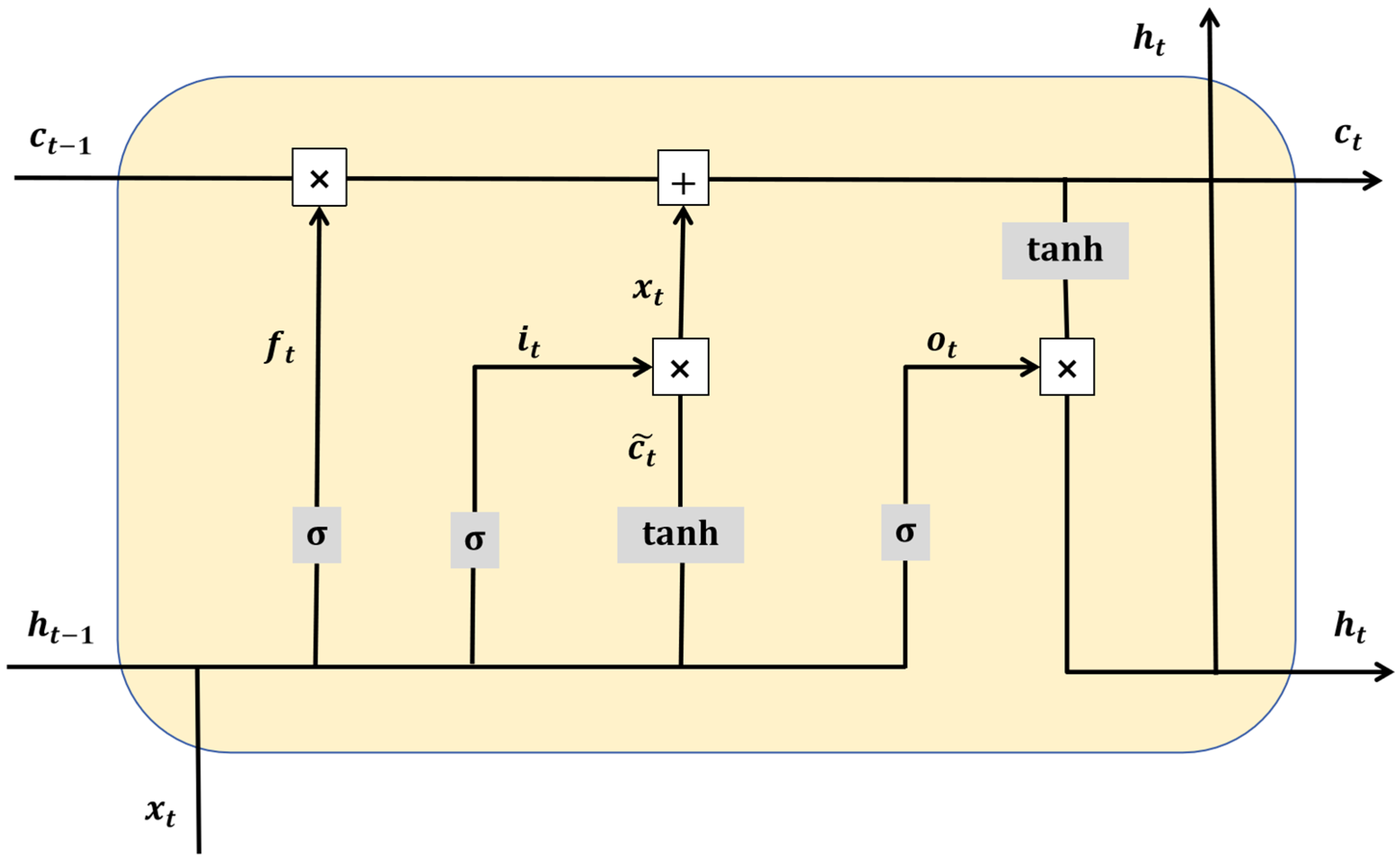
The LSTM neural network is specifically designed to capture long-term trends (e.g., interannual rising trends driven by global warming) and periodic patterns (e.g., seasonal cycles, ENSO event influences) in South China Sea level variations through its gated mechanisms (forget gate, input gate, output gate). This architecture is naturally suited for time-series prediction as it can effectively process long-term observational data from the region, including satellite altimeter records and tide gauge measurements. Temporal patterns in the data are automatically learned by the LSTM without requiring manual feature engineering, while its robustness in handling noise and missing values has been well demonstrated, enabling adaptation to imperfect real-world observational data. The northern South China Sea level dataset contains multiple periodic components. The LSTM’s capability to automatically learn temporal patterns without manual feature design makes it particularly suitable for processing such multi-scale periodic signals. A schematic diagram of the LSTM neural network is shown in Figure 5.

This figure shows the structure of the long short-term memory (LSTM) neural network. LSTM is a special type of recurrent neural network (RNN) designed to address the vanishing gradient problem that traditional RNNs face when dealing with long-sequence data.

The following are the main key components in the figure:

(1)

Input: x_t represents the input data at time step t. It is taken as input together with the hidden state h_t−1 from the previous time step.

(2)

Cell State: c_t−1 and ct represent the cell states of the previous time step and the current time step, respectively. The cell state is like a conveyor belt that passes information throughout the sequence. It has only a few linear interactions, which helps in maintaining long-term dependencies of information.

(3)

Gate Mechanisms

Forget Gate: Represented by ft, it determines which information to discard from the cell state c_t−1. ft is calculated through a σ (sigmoid) function, and the output value ranges from 0 to 1, where 0 means completely discarding and 1 means completely retaining.

Input Gate: Represented by i_t, it determines which new information to add to the cell state. It is also calculated through the σ function. $\widetilde{c_t}$ is a candidate value generated through the tanh function, which is used to update the cell state.

Output Gate: Represented by o_t, it determines which information from the cell state will be output as the hidden state h_t at the current time step; o_t is also calculated through the σ function, and then it is multiplied by the cell state value processed by tanh to obtain ht.

Hidden State: h_t−1 and h_t are the hidden states of the previous time step and the current time step, respectively. The hidden state is not only passed to the next time step but also used to generate the output.

Using the Adam gradient descent algorithm, the maximum training times are 1200 times, the initial learning rate is $5\times {10}^{-3}$, the learning rate reduction factor is 0.1, and the learning rate after 800 training times is $0.005\times 0.1$. After 800 epochs, the learning rate is decayed from 0.005 to 0.0005 to prevent excessively slow convergence in later stages. The Adam optimizer, when combined with learning rate decay, is demonstrated to effectively balance convergence speed and prediction accuracy. This approach is particularly suitable for LSTM networks processing non-stationary time-series data.

3. Sea Level Height Prediction Model Based on Harmonic Analysis

3.1. The Trend of Sea Level Variations in the Northern South China Sea

Based on the measured data from the Zhapo Ocean Station, the trend of sea level change is obtained by linear fitting (Figure 6). The sea level trend equation is shown in Equation (7). Over the past 44 years, the sea level in the northern South China Sea has shown an upward trend, and the rising rate is 1.4 mm/a.

$${\mathrm{y}}_{\mathrm{z}\mathrm{p}}=1.3852\times \mathrm{t}-630.5003$$

(7)

where ${\mathrm{y}}_{\mathrm{z}\mathrm{p}}$ represents the sea level height value for Zhapo corresponding to the year t.

During harmonic analysis, the data need to be detrended. The main purpose of detrending is to eliminate non-periodic trend components in the data so that periodic or harmonic signals can be extracted and analyzed more accurately. This paper uses linear fitting to detrend the data, as shown in Figure 6.

3.2. Harmonic Analysis of Sea Level Variations in the Northern South China Sea

This paper uses 20th-order harmonic components for spectral analysis and reconstruction of sea level height. Figure 7 shows the period–amplitude relationship of the first 20 harmonic components in the data, where the horizontal axis represents the harmonic period and the vertical axis represents the corresponding amplitude.

Table 1. Table of periods and corresponding amplitude values for 20 harmonic components.

Harmonic	Period (Years)	Amplitude
1	52	14.6589
2	26	8.8137
3	17.3333	9.4461
4	13	22.9499
5	10.4	7.9607
6	8.6667	4.5325
7	7.4286	4.6562
8	6.5	8.296
9	5.7778	9.0724
10	5.2	6.6983
11	4.7273	5.3255
12	4.3333	3.946
13	4	6.7548
14	3.7143	7.6679
15	3.4667	8.4842
16	3.25	3.6371
17	3.0588	1.894
18	2.8889	6.0964
19	2.7368	9.4715
20	2.6	9.9076

lists the periods and corresponding amplitude values of the 20 harmonic components. In historical records of sea level variations, long-term trends coexist with short-term fluctuations. In this study, the original time series is detrended using a linear fitting algorithm (implemented via MATLAB R2023b for data preprocessing), followed by harmonic analysis performed on the detrended residual fluctuation components. Based on amplitude analysis, the first four harmonic components are determined as the primary contributors to sea surface height variation in this paper, while the fifth to tenth harmonic components are classified as secondary influencing factors.

Harmonic analysis identifies four dominant oscillation modes of sea level variability in the northern South China Sea, with their corresponding period and amplitude parameters presented in

Table 2. Main components in northern South China Sea.

Main Components	f1 = 22.95 × sin(2 × π × 0.0769 × t − 0.13)	f2 = 14.66 × sin(2 × π × 0.0192 × t − 2.73)	f3 = 9.91 × sin(2 × π × 0.3846 × t + 0.60)	f4 = 9.47 × sin(2 × π × 0.3654 × t + 1.09)
Period	13.00	52.00	2.60	2.74
Amplitude	22.95	14.66	9.91	9.47

. Notably, these oscillation periods show remarkable consistency with solar activity cycles, suggesting that solar radiation variations may serve as a significant external forcing factor driving regional sea level fluctuations.

The prediction equation for the main components is calculated as shown in Equation (8), and the comparison between the main components and the measured values is shown in Figure 8. It shows the comparison between the predicted values of the main components and the observed values in the harmonic analysis. The horizontal axis in the figure represents the year (1970–2030), and the vertical axis represents the detrended sea level height (millimeters). “Detrended Data” indicates the original detrended data, while “Combined Main Components” represents the combined prediction results of the four main harmonic components. It can be seen from the figure that the prediction curve of the main components basically matches the fluctuation trend of the detrended data, indicating that the four main harmonic components can effectively characterize the periodic characteristics of sea level changes.

y1 = 22.95 × sin(2 × π × 0.0769 × t − 0.13) + 14.66 × sin(2 × π × 0.0192 × t − 2.73) + 9.91 × sin(2 × π × 0.3846 × t + 0.60) + 9.47 × sin(2 × π × 0.3654 × t + 1.09)

(8)

This paper employs a multilevel harmonic decomposition approach to predict sea surface height variations in the northern South China Sea. The methodological procedure consists of four key steps: (1) detrending preprocessing of the original data, (2) primary harmonic analysis for extracting dominant oscillation modes, (3) residual computation (detrended data minus principal wave components) to obtain secondary fluctuation series, and (4) higher-order harmonic analysis performed on the residual series to establish a comprehensive multi-scale prediction model. The period and amplitude parameters of the six secondary oscillation modes are presented in

Table 3. Secondary components in northern South China Sea.

Secondary components	f1′ = 9.45 × sin(2 × π × 0.0577 × t − 0.90)	f2′ = 9.22 × sin(2 × π × 0.4423 × t − 3.08)	f3′ = 9.07 × sin(2 × π × 0.1731 × t − 0.88)
Period	17.33	2.26	5.78
Amplitude	9.45	9.22	9.07
Secondary components	f4′ = 8.81 × sin(2 × π × 0.0385 × t + 0.30)	f5′ = 8.48 × sin(2 × π × 0.2885 × t + 0.24)	f6′ = 8.30 × sin(2 × π × 0.1538 × t − 2.22)
Period	25.97	3.47	6.50
Amplitude	8.81	8.48	8.30

.

The prediction equation for secondary oscillations is given in Equation (9), and the comparison between the secondary components and measured values is shown in Figure 9.

y2 = 9.45 × sin(2 × π × 0.0577 × t − 0.90) + 9.22 × sin(2 × π × 0.4423 × t − 3.08) + 9.07 × sin(2 × π × 0.1731 × t − 0.88) + 8.81 × sin(2 × π × 0.0385 × t + 0.30) + 8.48 × sin(2 × π × 0.2885 × t + 0.24) + 8.30 × sin(2 × π × 0.1538 × t − 2.22)

(9)

Figure 9 shows the comparison between the predicted values of the secondary components and the observed values in the harmonic analysis. The horizontal axis represents the year (1970–2030), and the vertical axis represents the detrended sea level height (millimeters). “Detrended Data” indicates the original detrended data, while “Combined Secondary Components” represents the combined prediction results of the six secondary harmonic components. The comparison demonstrates that the prediction curve of the secondary components can effectively capture the detailed fluctuations in the original data, indicating that higher-order harmonic analysis plays a significant role in improving the model’s accuracy.

Equation (10) is obtained by summing Equations (8) and (9).

$${\mathrm{y}}_{\left(\mathrm{d}\mathrm{p}\mathrm{r}\right)}={\mathrm{y}}_{\left(1\right)}+{\mathrm{y}}_{\left(2\right)}$$

(10)

Equation (10) represents the prediction equation for future sea level changes after detrending. To obtain the true sea level changes, the long-term trend formula in Equation (7) should also be added. The final prediction equation for future sea level changes is denoted as Equation (11).

$${\mathrm{H}}_{(\mathrm{p}\mathrm{r}.\mathrm{s}\mathrm{l})}={\mathrm{y}}_{\left(\mathrm{q}\mathrm{s}\right)}+{\mathrm{y}}_{\left(\mathrm{d}\mathrm{p}\mathrm{r}\right)}$$

(11)

In model evaluation, the root mean square error (RMSE), mean absolute error (MAE), coefficient of determination (R²), and mean bias error (MBE) are key metrics, with their formulas as follows:

$$\mathrm{R}\mathrm{M}\mathrm{S}\mathrm{E}=\sqrt{{\displaystyle \frac{1}{\mathrm{n}}}{\sum }_{\mathrm{i}=1}^{\mathrm{n}}{({\mathrm{y}}_{\mathrm{i}}-\widehat{{\mathrm{y}}_{\mathrm{i}}})}^2}$$

(12)

$$\mathrm{M}\mathrm{A}\mathrm{E}={\displaystyle \frac{1}{\mathrm{n}}}{\sum }_{\mathrm{i}=1}^{\mathrm{n}}\left|{\mathrm{y}}_{\mathrm{i}}-\widehat{{\mathrm{y}}_{\mathrm{i}}}\right|$$

(13)

$${\mathrm{R}}^2=1-{\displaystyle \frac{\frac{1}{\mathrm{n}}{\sum }_{\mathrm{i}=1}^{\mathrm{n}}{({\mathrm{y}}_{\mathrm{i}}-\widehat{{\mathrm{y}}_{\mathrm{i}}})}^2}{\frac{1}{\mathrm{n}}{\sum }_{\mathrm{i}=1}^{\mathrm{n}}{({\mathrm{y}}_{\mathrm{i}}-\overline{{\mathrm{y}}_{\mathrm{i}}})}^2}}$$

(14)

$$\mathrm{M}\mathrm{B}\mathrm{E}={\displaystyle \frac{1}{\mathrm{n}}}{\sum }_{\mathrm{i}=1}^{\mathrm{n}}({\mathrm{y}}_{\mathrm{i}}-\widehat{{\mathrm{y}}_{\mathrm{i}}})$$

(15)

where $\mathrm{n}$ is the number of samples, ${\mathrm{y}}_{\mathrm{i}}$ is the true value, and $\widehat{{\mathrm{y}}_{\mathrm{i}}}$ is the predicted value. $\overline{{\mathrm{y}}_{\mathrm{i}}}$ is the average of the true values, RMSE and MAE reflect the size of the prediction error, ${\mathrm{R}}^2$ measures the model’s goodness of fit to the data, and MBE is used to determine the overall deviation direction of the predicted values.

After secondary fluctuation components are introduced based on the main components, the predictive performance is significantly improved. Specifically, the correlation coefficient between the predicted and true values increases from 0.538 to 0.675, representing a 25.5% increase. Concurrently, the root mean square error (RMSE) decreases from 29.053 to 20.425, reflecting a 29.7% reduction. These quantitative indicator changes indicate that the inclusion of secondary fluctuation components effectively improves the model’s predictive accuracy.

Figure 10 illustrates the comparison between the sea level height prediction model based on harmonic analysis and the measured data. It is shown that the long-term trend and periodic fluctuations of sea level changes are effectively captured by the harmonic analysis model: the predicted curve is generally consistent with the overall trend of the measured data, particularly during 1970–2000, where the amplitude and periodic characteristics of the two are highly matched. Statistical metrics are presented as follows: the root mean square error (RMSE) is 14.73, the mean absolute error (MAE) is 12.61, and the coefficient of determination (R²) is 0.84. These metrics indicate a high goodness-of-fit, with 84% of the variance in sea level changes being explained by the model. However, certain deviations are exhibited by the model in partial periods after 2000 (e.g., 2010–2020), where the fluctuation amplitude of the measured data exceeds the predicted values. This phenomenon can potentially be attributed to the model’s insufficient capability to capture extreme climate events or high-frequency fluctuations. Overall, while the harmonic analysis model performs excellently in characterizing the main trends and periodic components of sea level changes, improvements are still needed in addressing complex nonlinear fluctuations.

4. Sea Level Height Prediction Model Based on Artificial Neural Network

During the process of establishing prediction models using the GA-BP, RBF, and LSTM neural networks, the dataset is first divided into training and testing sets in an 11:2 ratio. Then, the dataset needs to be normalized. The value of variable $x$ is normalized to obtain $x_{\mathrm{n}\mathrm{o}\mathrm{r}\mathrm{m}}$. The normalization equation is as follows:

$${\mathrm{x}}_{\mathrm{n}\mathrm{o}\mathrm{r}\mathrm{m}}={\displaystyle \frac{\mathrm{x}-\mathrm{m}\mathrm{i}\mathrm{n}\left(\mathrm{X}\right)}{\mathrm{m}\mathrm{a}\mathrm{x}\left(\mathrm{X}\right)-\mathrm{m}\mathrm{i}\mathrm{n}\left(\mathrm{X}\right)}}$$

(16)

The final predicted value ($x$) is obtained via de-normalization of $x_{\mathrm{n}\mathrm{o}\mathrm{r}\mathrm{m}}$. The de-normalization equation is as follows:

$$\mathrm{x}={\mathrm{x}}_{\mathrm{n}\mathrm{o}\mathrm{r}\mathrm{m}}·\left(\mathrm{m}\mathrm{a}\mathrm{x}\right(\mathrm{X})-\mathrm{m}\mathrm{i}\mathrm{n}(\mathrm{X}\left)\right)+\mathrm{m}\mathrm{i}\mathrm{n}\left(\mathrm{X}\right)$$

(17)

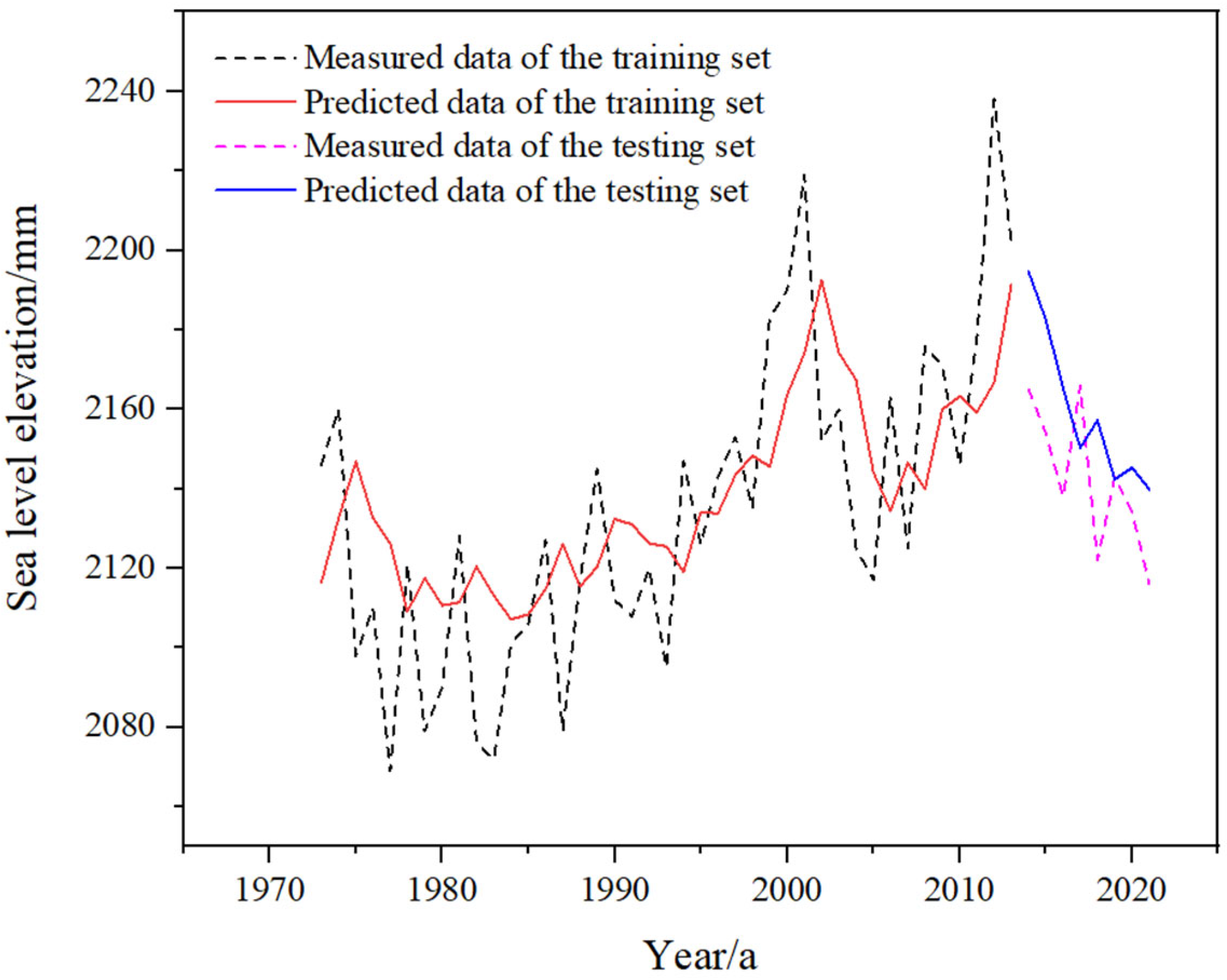
Figure 11 shows the prediction effects of the training set and testing set of the sea level height prediction model established based on the GA-BP neural network. The accuracy and robustness of the sea level height prediction model based on the GA-BP neural network are evaluated. The RMSE of the model is 29.1371, the MAE is 24.9411, the MBE is 5.6809, and the R² is 0.4003.

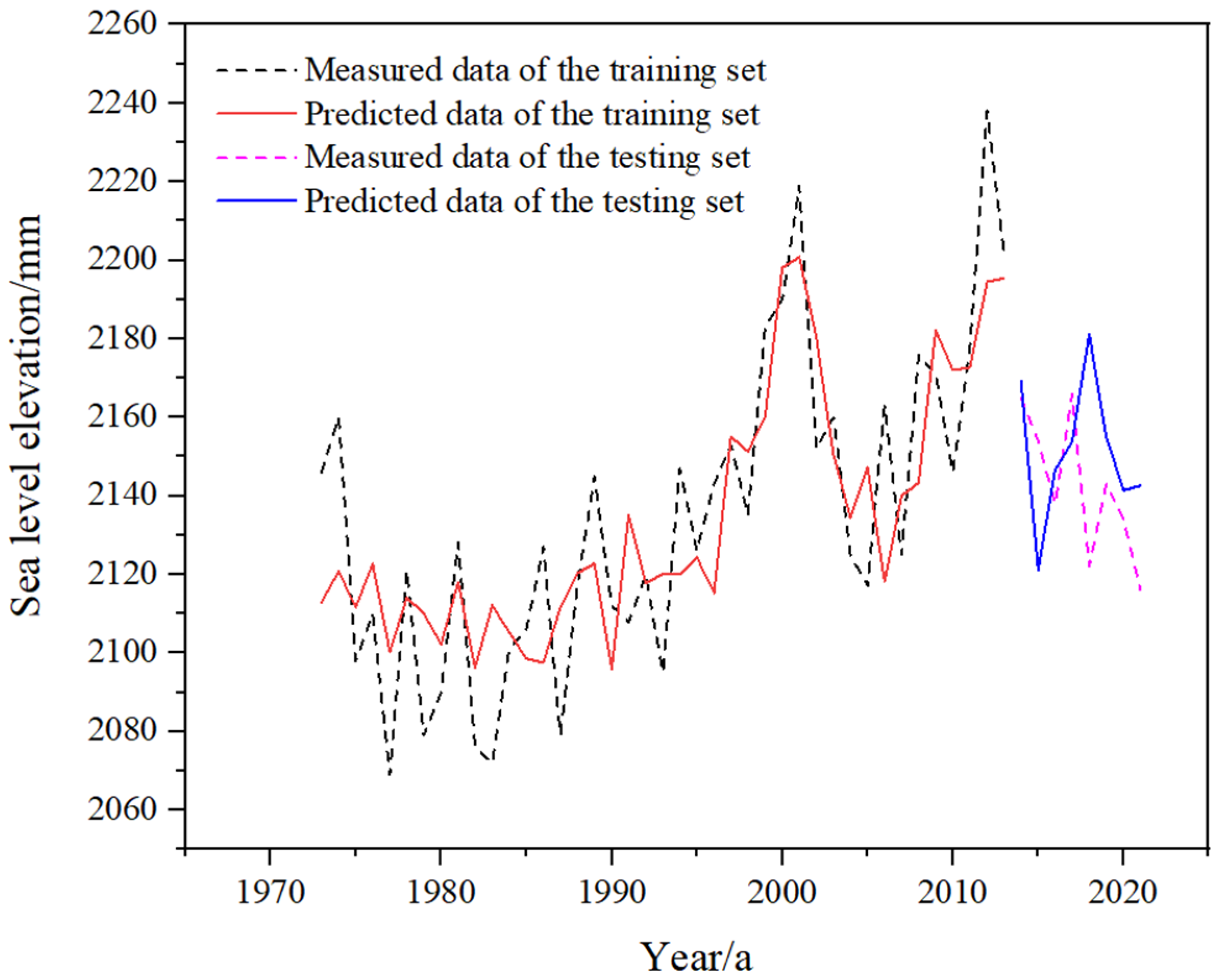
Figure 12 shows the prediction effects of the training set and testing set of the sea level height prediction model established based on the RBF neural network. The accuracy and robustness of the sea level height prediction model based on the RBF neural network are evaluated. The RMSE of the model is 27.1433, the MAE is 22.7533, the MBE is 2.1322, and the R² is 0.4690.

Figure 13 shows the prediction effects of the training set and testing set of the sea level height prediction model established based on the LSTM neural network. The accuracy and robustness of the sea level height prediction model based on the LSTM neural network are evaluated. The RMSE of the model is 23.7929, the MAE is 19.7899, the MBE is 1.3700, and the R² is 0.5872.

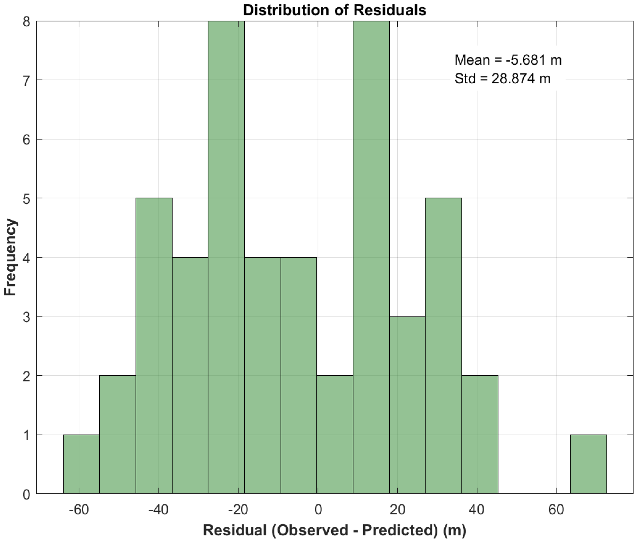
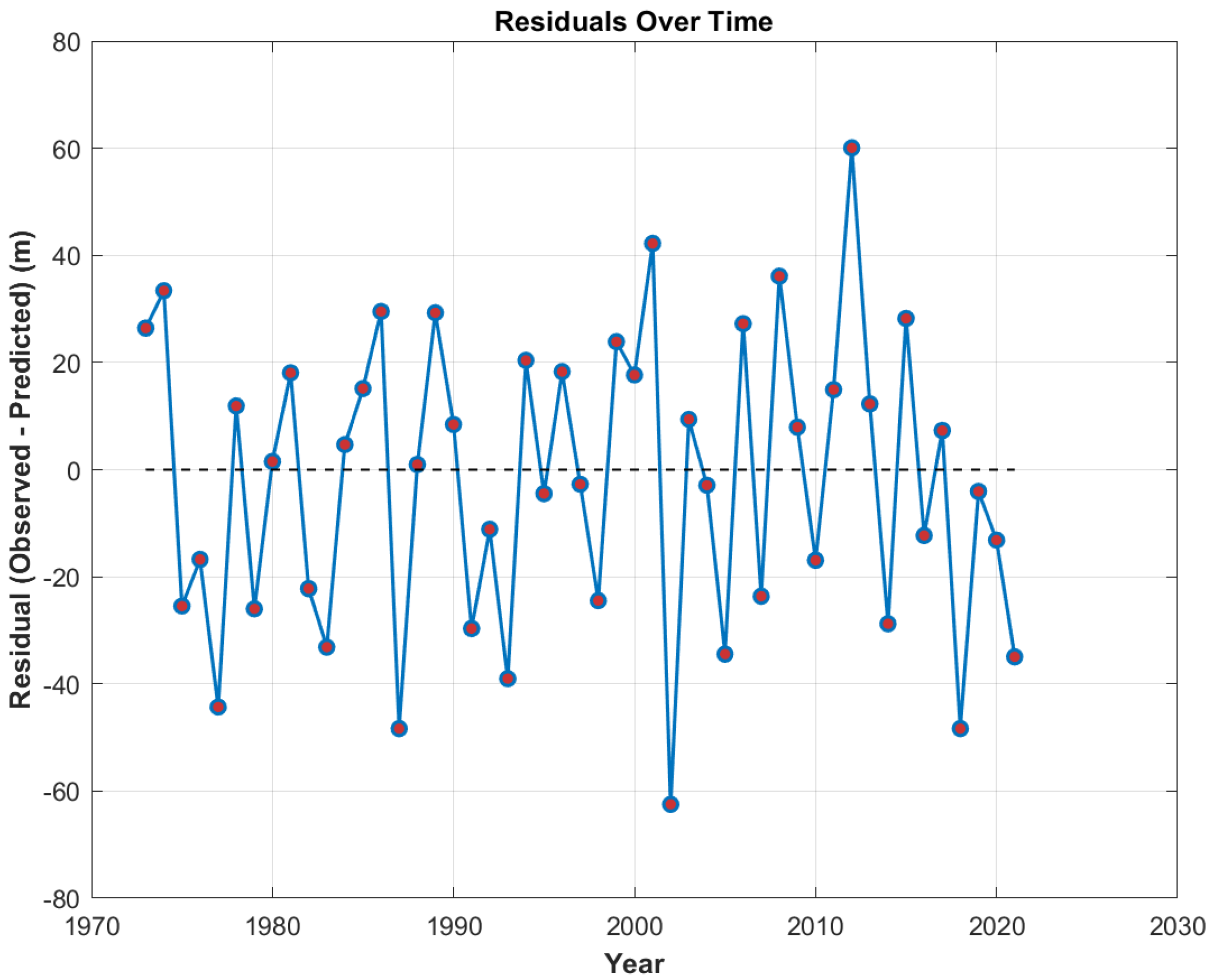
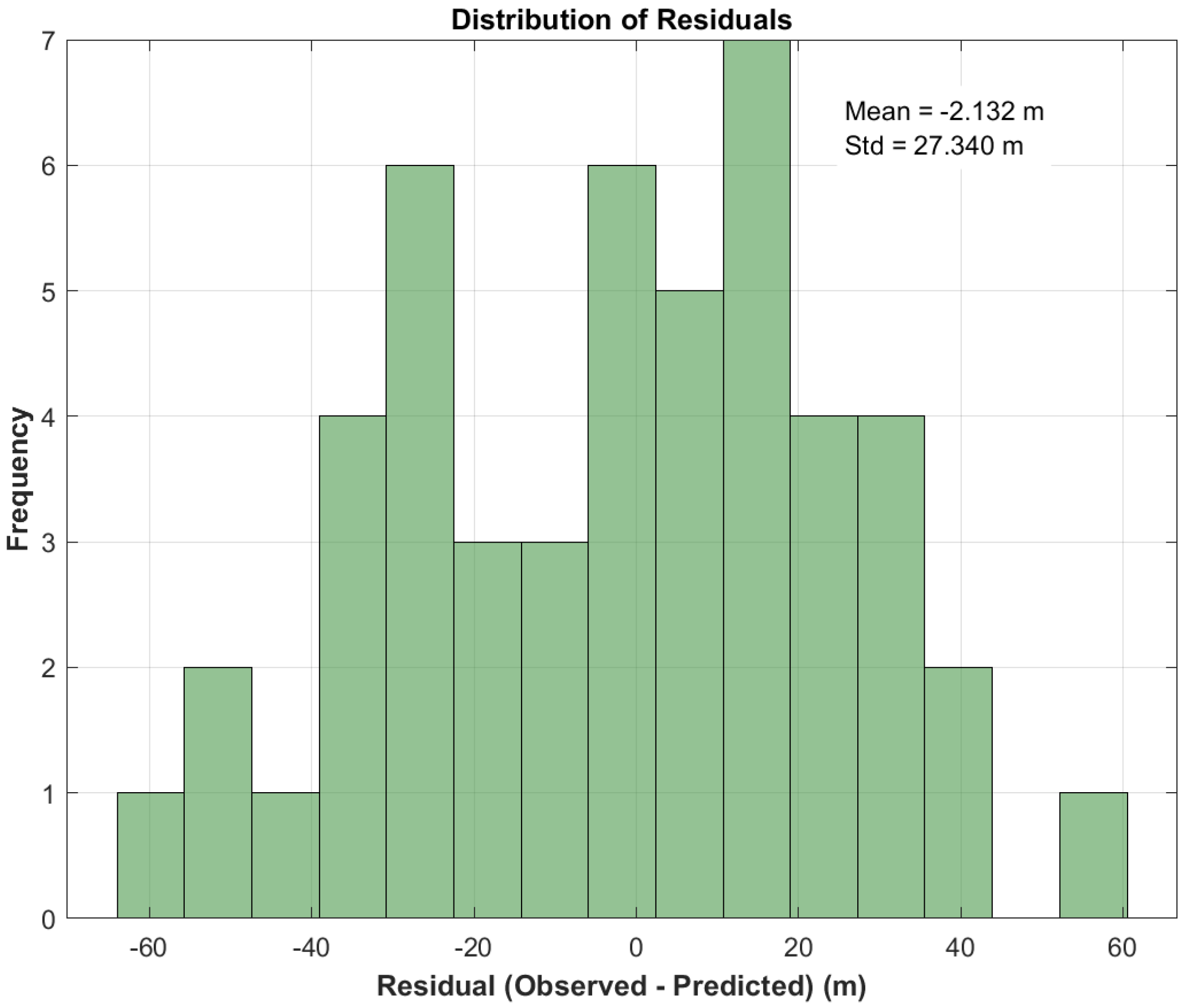
Figure 14 and Figure 15 show the relationship between residuals and time, and the distribution of residuals in the sea level prediction model based on harmonic analysis, respectively. Figure 16 and Figure 17 show the relationship between residuals and time, and the distribution of residuals in the sea level prediction model based on the GA-BP neural network, respectively. Figure 18 and Figure 19 show the relationship between residuals and time, and the distribution of residuals in the sea level prediction model based on the RBF neural network, respectively. 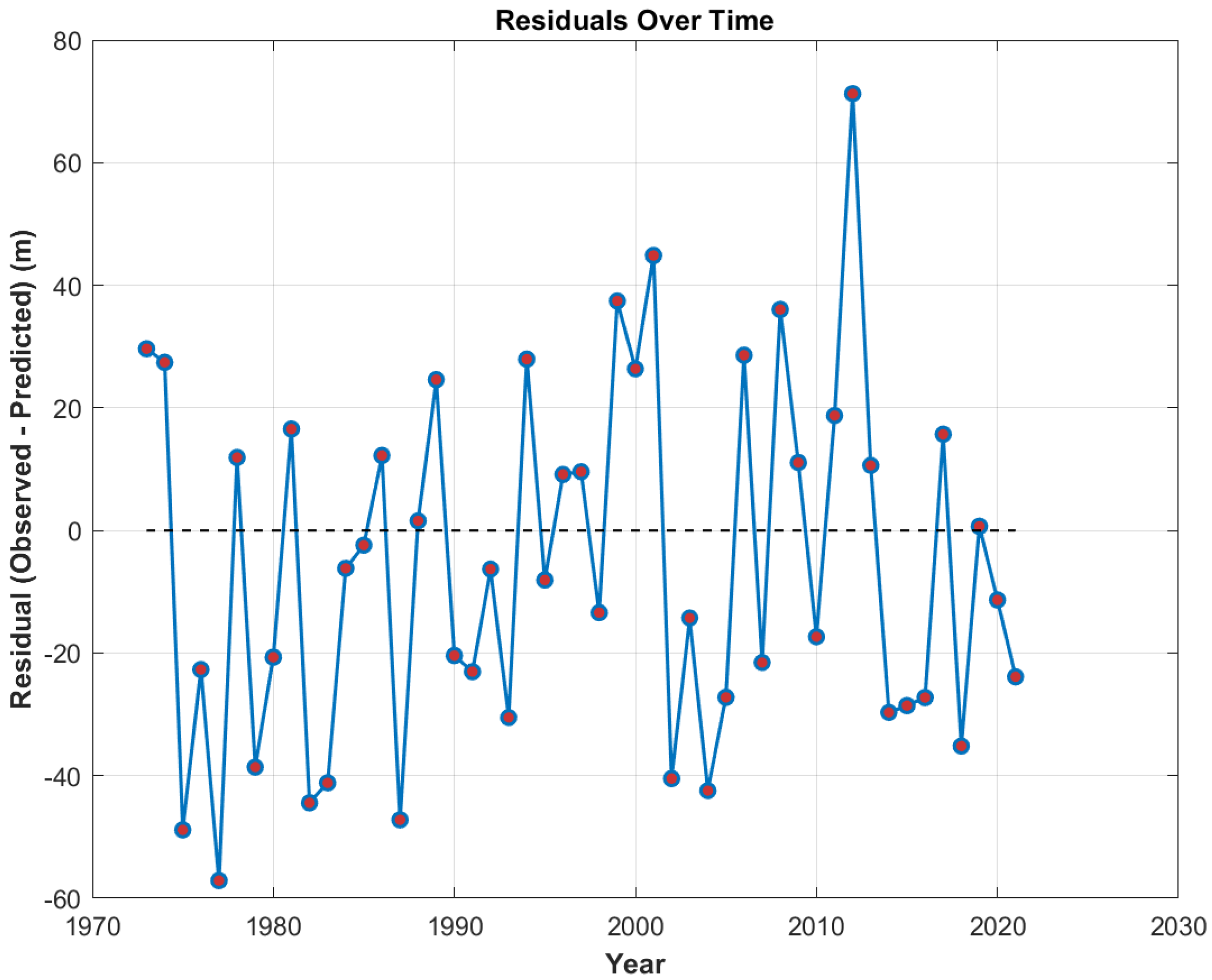Figure 20 and Figure 21 show the relationship between residuals and time, and the distribution of residuals in the sea level prediction model based on the LSTM neural network, respectively. The temporal variation of residuals is found to reveal periodic or systematic biases (e.g., long-term drift or transient anomalies). As shown in Figure 14, Figure 16, Figure 18 and Figure 20, the harmonic analysis model is observed to exhibit the smallest residual range (−36.8372 to 24.8940 m), followed by the LSTM neural network model (−59.1870 to 44.7200 m) and the RBF neural network model (−62.4861 to 60.0700 m). The most significant residual fluctuation is seen in the GA-BP model (−57.1122 to 71.2489 m), suggesting that overfitting or sensitivity to extreme values may be present in this model. The probability distributions of residuals are presented in Figure 15, Figure 17, Figure 19 and Figure 21. The results indicate that the residuals of harmonic analysis approximately follow a normal distribution (standard deviation: 14.8300 m), though a slight left skewness (mean: −0.2889 m) is noted, implying a potential minor negative bias. In contrast, the residual distributions of neural network models are more dispersed (standard deviation: 23–29 m), with the GA-BP model showing the largest standard deviation and mean values, demonstrating that this prediction model has the poorest robustness.

Table 4. The residual statistical parameters for the harmonic analysis, GA-BP neural network, RBF neural network, and LSTM neural network models.

	Harmonic Analysis	GA-BP Neural Network	RBF Neural Network	LSTM Neural Network
Mean residual	−0.2889	−5.6809	−2.1322	−1.3700
Standard deviation	14.8300	28.8741	27.3398	23.9996
RMS residual	14.6807	29.1371	27.1433	23.7929
Minimum residual	−36.8372	−57.1122	−62.4861	−59.1870
Maximum residual	24.8940	71.2489	60.0700	44.7200
Residual range	61.7311	128.3611	122.5562	103.9070

presents the residual statistical parameters for the harmonic analysis, GA-BP neural network, RBF neural network, and LSTM neural network models. The residual statistics in Table 4 reveal significant performance differences among the four modeling approaches for sea level prediction in the northern South China Sea. Harmonic analysis demonstrates superior stability with the smallest residual range, lowest standard deviation and RMS residual, and minimal systematic bias. Among the neural networks, the LSTM model shows the best performance with a relatively narrow residual range and lower standard deviation and RMS residual, suggesting its effectiveness in handling temporal patterns. The RBF network exhibits intermediate results with a residual range and standard deviation between those of the LSTM and GA-BP models. In contrast, the GA-BP network displays the weakest performance, characterized by the widest residual range, highest standard deviation and RMS residual, and largest systematic bias. These findings quantitatively demonstrate that while harmonic analysis provides the most reliable predictions, the LSTM neural network offers the best neural network alternative, particularly for applications requiring complex temporal pattern recognition. The substantial performance gaps, especially evident in residual ranges varying from 61.7311 m to 128.3611 m, underscore the critical importance of model selection for accurate sea level prediction in this region.

This section establishes sea level height prediction models based on the GA-BP, RBF, and LSTM neural networks. The statistical parameters of the neural network prediction model are shown in

Table 5. Statistical parameter table of neural network prediction model.

	GA-BP	RBF	LSTM	Harmonic Analysis
RMSE	29.1371	27.1433	23.7929	14.73
MAE	24.9411	22.7533	19.7899	12.61
MBE	5.6809	2.1322	1.3700	−0.0000
R2	0.4003	0.4690	0.5872	0.84

. We use four statistical indicators, RMSE, MAE, MBE, and R², to evaluate the accuracy and robustness of each model. These four calculation formulas are shown in Formulas (12)–(15). The results indicate that the harmonic analysis model achieves the highest accuracy and robustness among the three models.

Figure 22 shows the results of predicting sea level heights for the next decade (2023–2033) based on the harmonic analysis model. The results show that the rising trend of sea level will continue, and it is expected that the altitude will increase to about 2250–2300 mm by 2033. This prediction further supports the observed upward trend in historical data, highlighting the importance of conducting long-term sea level monitoring and disaster risk assessment.

5. Discussion

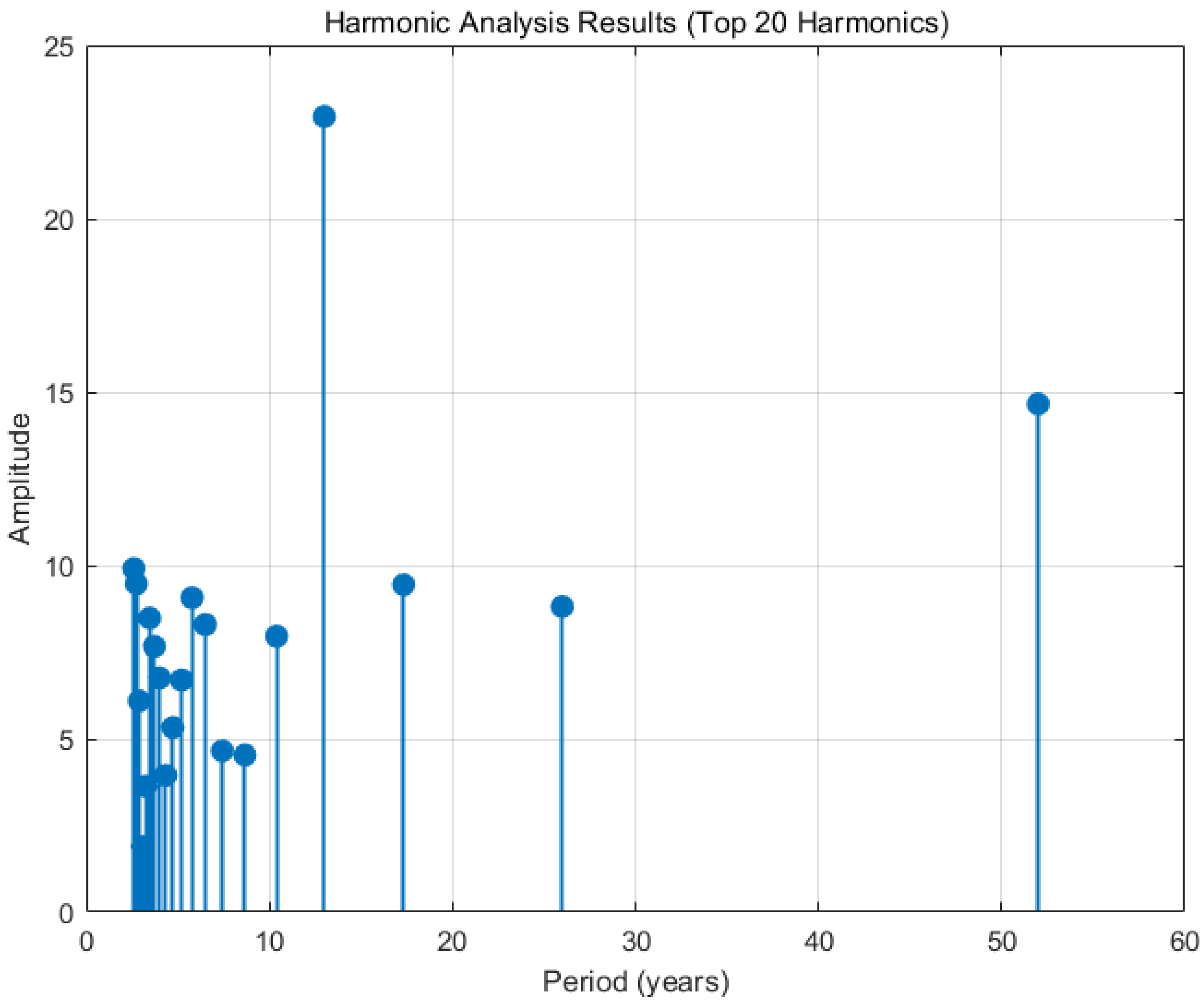
The robustness of the harmonic analysis method is validated through three aspects. First, compared with mainstream machine learning models such as GA-BP, RBF, and LSTM, harmonic analysis outperforms them in RMSE and MAE metrics (RMSE = 14.73 vs. LSTM = 23.79), indicating its stability across different modeling frameworks. Second, the long-term prediction results based on 52 years of full-period data show no significant error accumulation over time, verifying its adaptability to long-term trends. Finally, the consistency between model parameters and physical mechanisms such as solar activity cycles (13 years) and ENSO events (2–7 years) avoids the overfitting risk of purely data-driven models, further ensuring the reliability of the prediction results.

The accuracy and robustness of sea level height prediction models established using harmonic analysis and LSTM neural networks are evaluated through statistical metrics, including the RMSE, MAE, MBE, and R². The results indicate that the LSTM neural network achieves superior accuracy and robustness. This phenomenon can be attributed to the fact that sea level variations are primarily driven by strongly periodic factors such as tides and astronomical forces. Harmonic analysis, which models periodic signals directly through Fourier series or harmonic functions, excels at capturing fixed-frequency components. Specifically, when the data exhibit strong periodicity and low noise, the physics-based harmonic analysis outperforms the data-driven LSTM approach.

The superior performance of the harmonic analysis model in sea level prediction compared to artificial neural network (ANN) models can be primarily attributed to the alignment between data characteristics and model principles. The 52-year observational data used in this study exhibit significant periodicity (e.g., interannual and decadal fluctuations), and harmonic analysis directly models periodic signals through Fourier series, effectively separating trend terms and multi-scale periodic components (such as 13-year and 52-year main cycles) with clear physical meanings and strong noise resistance. In contrast, although ANN models (e.g., LSTM) excel at handling nonlinear data, their “black-box” nature leads to insufficient analytical capabilities for strong periodic signals and reliance on large amounts of data for training, prone to overfitting or degraded generalization when samples are limited.

The identification of dominant periodic components reveals the driving mechanisms of regional sea level changes. For example, the 52-year period closely aligns with the solar magnetic cycle (approximately 11 years) and its harmonic cycles (e.g., 55 years), suggesting that solar radiation modulation may drive long-term sea level fluctuations by influencing ocean heat budgets. The 13-year period may be related to the superposition effect of the quasi-period (approximately 2–7 years) of ENSO events, reflecting the remote impact of tropical Pacific air–sea interactions on the northern South China Sea. These periodic features provide an interpretable physical basis for prediction, helping to enhance model reliability.

The research results have important practical implications for coastal management and disaster prediction. The multi-scale periodic signals identified by harmonic analysis can be used to establish a hierarchical early warning system: for interannual cycles (such as short-term fluctuations caused by typhoon seasons), short-term forecasts can be optimized by integrating real-time tidal data; for decadal cycles (such as 13-year and 52-year trends), they can provide long-term scientific bases for coastal protection projects (e.g., breakwater design, sea level rise adaptation planning). Additionally, the high robustness of the model indicates that harmonic analysis can be a preferred prediction tool in regions with scarce data or limited real-time updates, assisting developing countries in enhancing their coastal vulnerability assessment capabilities.

Global climate warming directly leads to an increase in the Earth’s surface air temperature and ocean temperatures. Rising temperatures cause glaciers to melt, ultimately increasing the total ocean volume and leading to sea level rise. Additionally, the frequency of extreme weather events is also increasing. Tian et al. (2013) [34] conducted a study comparing the subtropical temperature in southern China with the global average temperature and global average sea surface temperature, finding an overall similar warming trend. The upward trend of sea levels in the northern South China Sea is roughly similar to the upward trends of global and subtropical temperatures and sea surface temperatures. Sea level rise is the positive feedback of climate warming and sea surface temperature increase, and the changes among the three are synchronous. Li et al. (2002) point out that an important cause of sea level rise in the South China Sea is the warming of upper ocean waters, and this trend may be related to decadal-scale changes in the warmer western Pacific pool nearby [35]. The South China Sea is located near the equator, and the sea level variations in its northern region are closely linked to the effects of the El Nino–Southern Oscillation (ENSO). During the selected time period for the study when El Nino events occurred, the sea level in the South China Sea was relatively low. Since ENSO and El Nino are companion events, ENSO is inevitably accompanied by overall oscillations, and El Nino events play a compensatory balancing role in sea level variations.

This study focuses on the comparison between traditional harmonic analysis and classical neural networks, with Transformer and other emerging architectures not being involved. Given the strong periodic characteristics of sea level variations in the northern South China Sea, the advantages of harmonic analysis are verified through physical mechanisms. Future research directions may include the following:

(1)

The self-attention mechanism of Transformer should be applied to long-term sea level data to capture non-periodic anomalous fluctuations (such as those influenced by typhoons and ENSO events);

(2)

Multi-source data (e.g., satellite altimetry and GRACE gravity field) should be incorporated to develop hybrid models for improving prediction accuracy in complex scenarios.

To further improve the prediction accuracy of the model, a hybrid model combining harmonic analysis and neural networks could be constructed in the future. Specifically, the periodic components obtained from harmonic decomposition could be used as the basis, while LSTM could be employed to predict the nonlinear residual terms. By integrating the strengths of both approaches, prediction accuracy in complex fluctuating scenarios can be enhanced. This study investigates sea level prediction using long-term tidal gauge data from the Zhapo Station in the northern South China Sea. While achieving important research outcomes, we must acknowledge several limitations: The single-station data cannot fully represent the spatial heterogeneity of sea level changes across the entire northern South China Sea region, and the absence of integrated multi-source data like satellite altimetry may affect the model’s generalizability to broader areas. The identified periodic characteristics require validation at other stations to confirm their universality, while the single data source presents challenges in resolving coupled signals between global climate change and regional ocean–atmosphere interactions. Future research will improve spatiotemporal representation by establishing multi-station observation networks, incorporating multi-source remote sensing data, and developing regionally calibrated models. These enhancements will help build a more robust regional sea level prediction system, providing more precise scientific support for comprehensive coastal zone management.

6. Conclusions

This comprehensive study of sea level variations in the northern South China Sea, based on 52 years of tidal data from the Zhapo Station (1970–2021), yields several significant scientific and practical insights. Through comparative analysis of harmonic decomposition and neural network approaches, we establish that sea levels have risen at 1.4 mm/year (95% CI: 1.1–1.7 mm/year) over the past 44 years, with the discrepancy from satellite altimetry estimates (3.5 mm/year) likely attributable to differences in observation periods and spatial scales. The superior performance of harmonic analysis, which effectively characterizes sea level variations through four main and six secondary components, challenges the prevailing assumption that complex machine learning models inherently outperform traditional methods in geophysical applications.

The scientific significance of these findings is threefold. First, the physically interpretable components of harmonic analysis provide a more reliable framework for long-term sea level forecasting than artificial neural networks in this context. Second, the identified 1.4 mm/year trend and dominant periodicities (potentially linked to ENSO and PDO) establish a critical baseline for climate change impact assessments. Third, our methodological comparison offers a rigorous benchmark for evaluating physics-based versus data-driven approaches in oceanographic studies.

These advances translate directly into practical applications for coastal management and climate adaptation. The multi-scale periodic signals enable the development of hierarchical protection systems, combining short-term early warning capabilities (e.g., for typhoon seasons) with long-term planning guidance (e.g., breakwater design based on 52-year cycles). The demonstrated accuracy of harmonic analysis supports its integration into risk assessment tools for designing adaptive infrastructure, while fisheries and maritime industries can leverage these forecasts to optimize operations and mitigate economic losses.

At the policy level, our findings provide actionable data for vulnerable coastal communities in monsoon Asia, supporting UN Sustainable Development Goal 13 (Climate Action). The 1.4 mm/year trend projection informs long-term coastal zoning and disaster preparedness planning, while the methodological framework—transferable to other tide-dominated regions like the Bay of Bengal and the Gulf of Mexico—facilitates international collaboration on coastal resilience strategies.

Future research should address the limitations of single-station data by incorporating multi-source observations (e.g., satellite altimetry, GRACE) and expanding to regional monitoring networks. This will enhance the spatial representativeness of predictions and further elucidate the complex interactions between global climate change and regional ocean–atmosphere dynamics in governing sea level variations.

References

1. Maxwell, K.; Rovere, A.; Westphal, H.; Garas, K.; Guinto, M.; Chauveau, D.; Hu, H.-M.; Shen, C.-C. Relative sea-level changes and reef development in the northern Coral Triangle during the late Quaternary. Geomorphology 2025, 483, 109796. [Google Scholar] [CrossRef]
2. Xu, J.H.; Guo, P.; Ma, Y.Q.; Jiang, C.; Liu, P.; Xu, W.; Li, C. Mechanism for the synchronous changes between lake level and global sea level during the Eocene warmhouse climate: Evidence from lacustrine carbonates. Palaeogeogr. Palaeoclim. Palaeoecol. 2025, 670, 112972. [Google Scholar] [CrossRef]
3. Uzun, P.; Otay, E.N. Sea-level change in Eastern Mediterranean, Aegean and Black seas analyzed at subregional scale of six CORDEX domains. Reg. Stud. Mar. Sci. 2025, 83, 104099. [Google Scholar] [CrossRef]
4. Daraz, U.; Bojnec, Š.; Khan, Y. The impact of climate change on migration patterns in coastal communities. Climate 2024, 12, 180. [Google Scholar] [CrossRef]
5. Khan, A.R.; Razak, M.S.B.A.; Yusuf, B.B.; Shafri, H.Z.B.M.; Mohamad, N.B. Harnessing artificial neural networks for coastal erosion prediction: A systematic review. Mar. Policy 2025, 178, 106704. [Google Scholar] [CrossRef]
6. Yan, H.; Sun, L.G.; Wang, Y.; Huang, W.; Qiu, S.; Yang, C. A record of the Southern Oscillation Index for the past 2,000 years from precipitation proxies. Nat. Geosci. 2011, 4, 611–614. [Google Scholar] [CrossRef]
7. Yue, Y.F.; Yu, K.F.; Tao, S.C.; Zhang, H.; Liu, G.; Wang, N.; Jiang, W.; Fan, T.; Lin, W.; Wang, Y. 3500-year western Pacific storm record warns of additional storm activity in a warming warm pool. Palaeogeogr. Palaeoclim. Palaeoecol. 2019, 521, 57–71. [Google Scholar] [CrossRef]
8. Chang, L.; Sun, W.K. Progress and prospect of sea level changes of global and China nearby seas. Rev. Geophys. Planet. Phys. 2021, 52, 266–279. [Google Scholar]
9. Mohamed, B.; Skliris, N. Recent sea level changes in the Red Sea: Thermosteric and halosteric contributions, and impacts of natural climate variability. Prog. Oceanogr. 2025, 231, 103416. [Google Scholar] [CrossRef]
10. Meli, M.; Marcaccio, M.; Mazzei, M.; Romagnoli, C. Temporal and spatial analysis of relative sea-level changes across the Emilia-Romagna coastal plain (northern Adriatic Sea). Estuar. Coast. Shelf Sci. 2025, 314, 109143. [Google Scholar] [CrossRef]
11. Xiao, M.; Jin, T.; Ding, H. A continuous piecewise polynomial fitting algorithm for trend changing points detection of sea level. Comput. Geosci. 2025, 196, 105876. [Google Scholar] [CrossRef]
12. Zhang, J.; Liu, J.; Zhang, X.; Yue, B.; Qiu, J. Mineralogy of the Yangtze (Changjiang) shoal: Implications for provenance and land-sea in-teraction response to sea level changes since MIS 6. Palaeogeogr. Palaeoclimatol. Palaeoecol. 2025, 664, 112813. [Google Scholar] [CrossRef]
13. Erkoç, M.H.; Doğan, U.; Simav, M.; Farımaz, İ. Coastal motion at tide gauge stations along the Black Sea coast from in-situ and space-based observations. Reg. Stud. Mar. Sci. 2025, 82, 104036. [Google Scholar] [CrossRef]
14. Ardalan, A.A.; Hashemifaraz, A. Tidal modeling based on satellite altimetry observations of TOPEX/Poseidon, Jason1, Jason2, and Jason3 with high prediction capability: A case study of the Baltic Sea. Geodesy Geodyn. 2025, 15, 404–418. [Google Scholar] [CrossRef]
15. Donlon, C.J.; Cullen, R.; Giulicchi, L.; Vuilleumier, P.; Francis, C.R.; Kuschnerus, M.; Simpson, W.; Bouridah, A.; Caleno, M.; Bertoni, R.; et al. The Copernicus Sentinel-6 mission: Enhanced continuity of satellite sea level measurements from space. Remote. Sens. Environ. 2021, 258, 112395. [Google Scholar] [CrossRef]
16. Zhang, Q.; Fu, X.G.; Su, S.H.; Zeng, S. Astronomical forcing of the paleoclimate and sedimentary noise modeling of sea-level changes in the Late Triassic. Palaeogeogr. Palaeoclim. Palaeoecol. 2025, 659, 112638. [Google Scholar] [CrossRef]
17. Liu, B.; Xu, S.; Yin, K. Spatial Inhomogeneity Analyses of Extreme Sea Levels along Lianyungang Coast Based on Numerical Simulation and Monte Carlo Model. Reg. Stud. Mar. Sci. 2024, 79, 103856. [Google Scholar] [CrossRef]
18. Jensen, D.A.; Nandan, V.; Mahoney, A.R.; Yackel, J.J.; Resler, L.M. Landfast sea ice break out patterns in the northern Bering Sea observed from C-band Synthetic Aperture Radar. Int. J. Appl. Earth Obs. Geoinf. 2023, 117, 103183. [Google Scholar] [CrossRef]
19. Aoki, S. Coherent sea level response to the Antarctic Oscillation. Geophys. Res. Lett. 2002, 29, 11-1–11-4. [Google Scholar] [CrossRef]
20. Hünicke, B.; Luterbacher, J.; Pauling, A.; Zorita, E. Regional differences in winter sea level variations in the Baltic Sea for the past 200 yr. Tellus A 2010, 60, 384–393. [Google Scholar] [CrossRef]
21. Liu, H.; Cheng, X.; Qin, J.; Zhou, G.; Jiang, L. The dynamic mechanism of sea level variations in the Bohai Sea and Yellow Sea. Clim. Dyn. 2023, 61, 2937–2947. [Google Scholar] [CrossRef]
22. Hochet, A.; Llovel, W.; Huck, T.; Sévellec, F. Advection surface-flux balance controls the seasonal steric sea level amplitude. Sci. Rep. 2024, 14, 10644. [Google Scholar] [CrossRef]
23. Wang, O.; Lee, T.; Frederikse, T.; Ponte, R.M.; Fenty, I.; Fukumori, I.; Hamlington, B.D. What Forcing Mechanisms Affect the Interannual Sea Level Co-Variability Between the Northeast and Southeast Coasts of the United States? J. Geophys. Res. Ocean. 2024, 129, e2023JC019873. [Google Scholar] [CrossRef]
24. Zhang, L.; Delworth, T.L.; Yang, X.; Zeng, F.; Gu, Q.; Li, S. Causes and multiyear predictability of the rapid acceleration of U.S. Southeast Sea level rise after 2010. Npj Clim. Atmos. Sci. 2024, 7, 113. [Google Scholar] [CrossRef]
25. Zhao, J.; Cai, R.; Fan, Y. Prediction of Sea Level Nonlinear Trends around Shandong Peninsula from Satellite Altimetry. Sensors 2019, 19, 4770. [Google Scholar] [CrossRef] [PubMed]
26. Zhang, L.; Delworth, T.L.; Yang, X.; Zeng, F. Skillful multiyear to decadal predictions of sea level in the North Atlantic Ocean and U.S. East Coast. Commun. Earth Environ. 2023, 4, 420. [Google Scholar] [CrossRef]
27. Deepa, J.S.; Gnanaseelan, C. On the skill of Indo-Pacific decadal sea level predictions and its connection with skilful AMO and PDO predictions. Clim. Dyn. 2024, 62, 10363–10380. [Google Scholar] [CrossRef]
28. Gu, Q.; Zhang, L.; Jia, L.; Delworth, T.L.; Yang, X.; Zeng, F.; Cooke, W.F.; Li, S. Exploring multiyear-to-decadal North Atlantic sea level predictability and prediction using machine learning. NPJ Clim. Atmos. Sci. 2024, 7, 255. [Google Scholar] [CrossRef]
29. Sun, Q.; Wan, J.; Liu, S. Estimation of Sea Level Variability in the China Sea and Its Vicinity Using the SARIMA and LSTM Models. IEEE J. Sel. Top. Appl. Earth Obs. Remote. Sens. 2020, 13, 3317–3326. [Google Scholar] [CrossRef]
30. Hyun, S.K.; Kim, S.E.; Jin, J.Y.; Do, J.D. Numerical Simulation of Water Level Change at the Coastal Area in the East Sea with the Inverted Barometer Effect. J. Korean Soc. Coast. Ocean Eng. 2016, 28, 13–26. [Google Scholar] [CrossRef]
31. Lee, T.L.; Makarynskyy, O.; Shao, C.C. A combined harmonic analysis-artificial neural network methodology for tidal predic-tions. J. Coast. Res. 2007, 23, 764–770. [Google Scholar] [CrossRef]
32. Voinov, G.N. Harmonic analysis of tides from standard observations of the sea level. Russ. Meteorol. Hydrol. 2009, 34, 464–472. [Google Scholar] [CrossRef]
33. Hieronymus, M.; Hieronymus, J.; Hieronymus, F. On the Application of Machine Learning Techniques to Regression Problems in Sea Level Studies. J. Atmospheric Ocean. Technol. 2019, 36, 1889–1902. [Google Scholar] [CrossRef]
34. Tian, C.C.; Chen, T.; Yu, K.F. Phased, periodic, and trend characteristics of temperature changes in South Subtropical China during 1901–2011. Mar. Geol. Quat. Geol. 2013, 33, 9–18. [Google Scholar] [CrossRef]
35. Li, L.; Xu, J.D.; Cha, R.S. Rising trend of South China Sea level in the 1990s: Observations from satellite altimetry. Chin. Sci. Bull. 2002, 47, 59–62. [Google Scholar]
Figure 3. GA-BP neural network.
Sustainability 17 06081 g003
Figure 5. LSTM neural network.
Sustainability 17 06081 g005
Figure 6. Detrending of sea level height data.
Sustainability 17 06081 g006
Figure 7. Period–amplitude relationship of top 20 harmonic constituents.
Sustainability 17 06081 g007
Figure 8. Comparison between main components’ prediction values and observed values in harmonic analysis.
Sustainability 17 06081 g008
Figure 9. Comparison between secondary components’ prediction values and observed values in harmonic analysis.
Sustainability 17 06081 g009
Figure 10. Comparison between harmonic analysis predicted values and observed values.
Sustainability 17 06081 g010
Figure 11. The effectiveness of the training and testing sets for sea level height prediction based on the GA-BP neural network.
Sustainability 17 06081 g011
Figure 12. The effect of the training and testing sets for sea level height prediction based on the RBF neural network.
Sustainability 17 06081 g012
Figure 13. The effect of the training and testing sets for sea level height prediction based on the LSTM neural network.
Sustainability 17 06081 g013
Figure 14. Residuals vs. time for sea level prediction model based on harmonic analysis.
Sustainability 17 06081 g014
Figure 15. Residual distribution of sea level prediction model based on harmonic analysis.
Sustainability 17 06081 g015
Figure 16. Residuals vs. time for sea level prediction model based on GA-BP neural network.
Sustainability 17 06081 g016
Figure 17. Residual distribution of sea level prediction model based on GA-BP neural network.
Sustainability 17 06081 g017
Figure 18. Residuals vs. time for sea level prediction model based on RBF neural network.
Sustainability 17 06081 g018
Figure 19. Residual distribution of sea level prediction model based on RBF neural network.
Sustainability 17 06081 g019
Figure 20. Residuals vs. time for sea level prediction model based on LSTM neural network.
Sustainability 17 06081 g020
Figure 21. Residual distribution of sea level prediction model based on LSTM neural network.
Sustainability 17 06081 g021
Figure 22. Sea level elevation prediction for the northern South China Sea from 2023 to 2033 based on the harmonic analysis model.
Sustainability 17 06081 g022