Dependent-Chance Goal Programming for Sustainable Supply Chain Design: A Reinforcement Learning-Enhanced Salp Swarm Approach

Abstract

The Sustainable Supply Chain Network Design Problem (SSCNDP) is to determine the optimal network configuration and resource allocation that achieve the trade-off among economic, environmental, social, and resilience objectives. The Sustainable Supply Chain Network Design Problem (SSCNDP) involves determining the optimal network configuration and resource allocation that allows trade-off among economic, environmental, social, and resilience objectives. This paper addresses the SSCNDP under hybrid uncertainty, which combines objective randomness got from historical data, and subjective beliefs induced by expert judgment. Building on chance theory, we formulate a dependent-chance goal programming model that specifies target probability levels for achieving sustainability objectives and minimizes deviations from these targets using a lexicographic approach. To solve this complex optimization problem, we develop a hybrid intelligent algorithm that combines uncertain random simulation with Reinforcement Learning-enhanced Salp Swarm Optimization (RL-SSO). The proposed RL-SSO algorithm is benchmarked against standard metaheuristics—Genetic Algorithm (GA), Particle Swarm Optimization (PSO), Differential Evolution (DE), and standard SSO, across diverse problem instances. Results show that our method consistently outperforms these techniques in both solution quality and computational efficiency. The paper concludes with managerial insights and discusses limitations and future research directions.

1. Introduction

Supply Chain Network Design (SCND) is a critical strategic decision that, when effectively implemented, enhances operational efficiency, cost competitiveness, and sustainability across the entire value network [1,2]. As global supply chains become increasingly complex and interconnected, they face escalating challenges, such as market volatility, regulatory pressures, environmental concerns, and disruptive events. These challenges demand simultaneous consideration of economic, environmental, social, and resilience objectives [3]. Recent disruptions, such as the COVID-19 pandemic, geopolitical tensions, and climate-related crises, have exposed the limitations of traditional deterministic planning methods and underscored the urgent need for robust supply chain designs that perform reliably under diverse and often conflicting sources of uncertainty [4].

Recent industry reports quantify the magnitude of these disruptions. According to McKinsey & Company [5], supply chain disruptions cost companies an average of 45% of one year’s profits per decade, translating to $150–300 million annually for Fortune 500 companies. Environmental impacts are equally significant: traditional supply chains account for 60% of global carbon emissions (approximately 36 billion tons CO₂ annually), with inefficient network designs contributing an additional 15–20% excess emissions [6]. Social impacts include the loss of 2.7 million manufacturing jobs in developed economies between 2019–2023 due to inadequate supply chain resilience, while creating precarious employment conditions for 40 million workers in developing nations [7]. These quantitative indicators underscore the urgent need for innovative optimization approaches that can simultaneously address economic, environmental, and social objectives under uncertainty.

Real-world supply chains are characterized by hybrid uncertainty, which simultaneously encompasses both aleatory uncertainty (arising from inherent randomness such as demand fluctuations and lead times) and epistemic uncertainty (stemming from incomplete knowledge, expert opinions, or qualitative risk assessments) [8,9]. This dual nature of uncertainty is particularly evident in complex decision-making scenarios: demand forecasting in emerging markets relies on both historical sales data representing objective randomness and expert assessments of market trends reflecting subjective beliefs, while supplier reliability evaluation integrates quantitative performance metrics with qualitative judgments about management capability or geopolitical risk.

Despite the prevalence of hybrid uncertainty in practice, traditional optimization approaches address these uncertainty types in isolation, each with inherent limitations. Stochastic programming effectively captures aleatory uncertainty through probability distributions [10], while robust optimization accounts for epistemic uncertainty by considering worst-case scenarios [11], and fuzzy programming incorporates subjective judgments through membership functions [12]. However, these single-paradigm methods prove inadequate when confronted with hybrid uncertainty environments. Probability theory struggles to model epistemic components, as it requires well-defined distributions that may not exist for expert judgments and belief-based assessments. Conversely, fuzzy theory lacks the mathematical rigor necessary to effectively handle data-driven randomness and may yield suboptimal or counterintuitive outcomes [13]. These fundamental limitations underscore the critical need for a unified paradigm capable of rigorously representing and optimizing under both uncertainty types within a single coherent framework.

At the heart of this challenge lies the issue of hybrid uncertainty, which encompasses both aleatory and epistemic components. The traditional approaches to supply chain optimization deal with uncertainty types in isolation: stochastic programming captures randomness in demand [10], robust optimization accounts for worst-case scenarios [11], and fuzzy programming incorporates subjective judgments [12]. In fact, real-world supply chains commonly exhibit hybrid uncertainty, combining aleatory uncertainty (arising from inherent randomness, such as demand fluctuations and lead times) and epistemic uncertainty (stemming from incomplete knowledge, expert opinion, or qualitative risk assessments) [8,9]. For instance, demand forecasting in emerging markets often relies on both historical sales data (objective randomness) and expert assessments of market trends (subjective belief). Similarly, evaluation of supplier reliability integrates quantitative performance metrics with qualitative judgments about management capability or political risk.

Single-paradigm methods fall short in such settings or environments. Probability theory struggles to model epistemic uncertainty, as it requires well-defined distributions that may not exist for expert judgments and belief-based assessments. Conversely, fuzzy theory lacks the mathematical rigor to effectively handle data-driven randomness, and it is susceptible to result in suboptimal or counterintuitive outcomes [13]. These limitations highlight the need for a unified paradigm capable of rigorously representing and optimizing under both types of uncertainty using a single model.

Chance theory, established and improved by Liu [13,14], possesses precisely this mathematical foundation by unifying the probability measures and the uncertainty measures within a single chance measure framework. The innovation of the chance theory is that it can maintain the mathematical richness of probability theory for objective randomness and still provide a uniform representation of subjective beliefs, so that more realistic and reliable modeling of hybrid uncertain environments is possible. This satisfies the basic restriction of traditional approaches by recognizing that supply chain parameters such as demand forecasts, supplier capacities, and risk analysis entail data-driven randomness and expert judgment-based beliefs [15]. Despite its theoretical strength, the application of chance theory to multi-objective sustainable supply chain planning remains largely unexplored. This gap presents a significant opportunity to enhance both theoretical insights and practical decision-making tools in the field. A particularly promising direction is the use of dependent-chance modeling, which shifts the focus from merely ensuring constraint satisfaction under fixed confidence levels to maximizing the probability of achieving sustainability objectives. Unlike chance-constrained programming, where the focus is on guaranteeing feasibility under specified confidence levels, dependent-chance goal programming enables a more goal-oriented and interpretable decision-making framework. It allows direct optimization of probabilistic target achievements, thus supporting more transparent strategic planning and richer trade-off analyses across sustainability dimensions [16].

The complexity of dependent-chance programming formulations, particularly when involving multiple sustainability objectives, creates a high computational workload that exceeds the one of traditional exact optimization methods [17]. These problems often exhibit non-convex and multi-modal objective spaces, necessitating sophisticated optimization strategies capable of effectively balancing exploration and exploitation based on highly intricate objective functions involving probability maximization.

While metaheuristic algorithms have shown promise in addressing such complex optimization problems, they are often limited by premature convergence and inability to adjust their search strategy based on problem characteristics [18].

Salp Swarm Optimization (SSO), introduced by [19], is a metaheuristic that offers desirable features alongside continuous optimization through its bio-inspired mechanism of chain formation and nature-based equilibrium between exploration and exploitation phases. However, traditional SSO employs static parameter settings that may not be optimal at any stage of the optimization, particularly with the dynamic solution landscapes of dependent-chance problems, where the optimum search strategy might be very different for different stages of the optimization.

To overcome this limitation, the integration of reinforcement learning (RL) with metaheuristics offers a promising path forward. RL provides a mechanism for adaptive parameter tuning and allows the optimization process to learn effective search behaviors by interacting with the environment [20]. Crucially, RL recognizes that different stages of the optimization require different strategies, i.e., aggressive exploration in the early stages to locate promising regions, and focused exploitation in later stages to refine solutions. By formulating parameter selection as a sequential decision-making problem, RL can dynamically adjust the exploration-exploitation trade-off based on real-time search feedback, thus improving both convergence speed and solution quality in dependent-chance optimization tasks [21,22].

To address the interconnected challenges and knowledge gaps in sustainable supply chain optimization under hybrid uncertainty, this paper proposes a unified framework that combines dependent-chance goal programming with a reinforcement learning-enhanced Salp Swarm Optimization (RL-SSO) algorithm. Our integrated approach makes the following key contributions:

1.

Hybrid Uncertainty Modeling Framework: We develop a mathematically grounded framework based on chance theory that is able to tackle the coexistence of random uncertainty due to historical information and belief-based uncertainty due to experts’ judgment in sustainable supply chain network design. This approach avoids the pitfalls of misapplying single-paradigm methods to inherently hybrid supply chain environments.

2.

Dependent-Chance Goal Programming Model: We propose a multi-objective optimization model that leverages dependent-chance programming to maximize the probability of achieving sustainability targets across four dimensions: economic efficiency, environmental impact, social responsibility, and resilience. The model provides intuitive, probability-based performance metrics for decision-makers operating under hybrid uncertainty.

3.

Adaptive Metaheuristic Algorithm: We design a novel RL-enhanced Salp Swarm Optimization algorithm that dynamically adapts its search strategy using reinforcement learning. This enables efficient navigation of the complex, non-convex search space typical of dependent-chance problems, with more manageable, probability-based performance metrics for decision-makers under hybrid uncertainty, while improving convergence behavior and solution quality.

4.

Computational Validation and Analysis: We conduct large-scale computational experiments on varying size and uncertainty levels, comparing with state-of-the-art optimization methods to demonstrate superior performance in terms of solution quality, computational efficiency, and robustness to changing problem characteristics.

5.

Practical Decision Support Framework: We provide managerial insights and sensitivity analyses that translate theoretical contributions into operational guidance for supply chain practitioners, including probability threshold selection strategies, quantification of trade-offs between sustainability dimensions, and guidelines for implementing hybrid uncertainty assessment.

The remainder of this paper is organized as follows: Section 2 presents the mathematical formulation of our sustainable supply chain network design problem, as well as the dependent-chance goal programming approach to multi-objective optimization under hybrid uncertainty. Section 3 provides the theoretical foundations of uncertain random theory for hybrid uncertainty modeling and chance measure calculation. Section 4 illustrates the hybrid intelligent algorithm, which integrates uncertain random simulations and reinforcement learning-based Salp Swarm Optimization for solving the dependent-chance goal programming model. Section 5 presents comprehensive numerical results and analyses, including algorithm performance comparisons, sensitivity analyses, and network structure observations across a various test instances. Section 6 summarizes the main findings, theoretical contributions, managerial implications, limitations, and future research opportunities.

2. Mathematical Model Formulation

Our mathematical model for sustainable supply chain network design under uncertainty uses the following uncertain random variables to represent hybrid uncertainties to enable the simultaneous optimization of multiple sustainability objectives.

2.1. Sets and Indices

$$\begin{array}{cccc}\hfill S& =\{1,2,...,s\}\hfill & \hfill & \mathrm{Set}\mathrm{of}\mathrm{suppliers}\hfill \\ \hfill M& =\{1,2,...,m\}\hfill & \hfill & \mathrm{Set}\mathrm{of}\mathrm{manufacturing}\mathrm{plants}\hfill \\ \hfill W& =\{1,2,...,w\}\hfill & \hfill & \mathrm{Set}\mathrm{of}\mathrm{warehouses}\hfill \\ \hfill D& =\{1,2,...,d\}\hfill & \hfill & \mathrm{Set}\mathrm{of}\mathrm{distribution}\mathrm{centers}\hfill \\ \hfill C& =\{1,2,...,c\}\hfill & \hfill & \mathrm{Set}\mathrm{of}\mathrm{customers}\hfill \\ \hfill R& =\{1,2,...,r\}\hfill & \hfill & \mathrm{Set}\mathrm{of}\mathrm{raw}\mathrm{materials}\hfill \\ \hfill P& =\{1,2,...,p\}\hfill & \hfill & \mathrm{Set}\mathrm{of}\mathrm{products}\hfill \\ \hfill T& =\{1,2,...,t\}\hfill & \hfill & \mathrm{Set}\mathrm{of}\mathrm{time}\mathrm{periods}\hfill \\ \hfill K& =\{1,2,...,k\}\hfill & \hfill & \mathrm{Set}\mathrm{of}\mathrm{disruption}\mathrm{scenarios}\hfill \\ \hfill E& =\{1,2,...,e\}\hfill & \hfill & \mathrm{Set}\mathrm{of}\mathrm{environmental}\mathrm{impact}\mathrm{categories}\hfill \\ \hfill N& =S\cup M\cup W\cup D\hfill & \hfill & \mathrm{Set}\mathrm{of}\mathrm{all}\mathrm{nodes}\mathrm{in}\mathrm{the}\mathrm{network}\hfill \\ \hfill L& =\{1,2,...,l\}\hfill & \hfill & \mathrm{Set}\mathrm{of}\mathrm{transportation}\mathrm{modes}\hfill \\ \hfill G& =\{1,2,...,g\}\hfill & \hfill & \mathrm{Set}\mathrm{of}\mathrm{sustainability}\mathrm{goals}\hfill \end{array}$$

2.2. Uncertain Parameters

2.2.1. Economic Parameters

$$\begin{array}{cc}\hfill {\widetilde{SC}}_{ij}& :\mathrm{Uncertain}\mathrm{supply}\mathrm{cost}\mathrm{from}\mathrm{supplier}i\mathrm{to}\mathrm{plant}j\hfill \\ \hfill {\widetilde{PC}}_{jk}& :\mathrm{Uncertain}\mathrm{production}\mathrm{cost}\mathrm{of}\mathrm{product}k\mathrm{at}\mathrm{plant}j\hfill \\ \hfill {\widetilde{TC}}_{ijkl}& :\mathrm{Uncertain}\mathrm{transportation}\mathrm{cost}\mathrm{of}\mathrm{product}k\mathrm{from}\mathrm{node}i\mathrm{to}\mathrm{node}j\mathrm{using}\mathrm{mode}l\hfill \\ \hfill {\widetilde{IC}}_{ik}& :\mathrm{Uncertain}\mathrm{inventory}\mathrm{holding}\mathrm{cost}\mathrm{of}\mathrm{product}k\mathrm{at}\mathrm{node}i\hfill \\ \hfill {\widetilde{FC}}_i& :\mathrm{Uncertain}\mathrm{fixed}\mathrm{cost}\mathrm{of}\mathrm{opening}\mathrm{facility}\mathrm{at}\mathrm{location}i\hfill \\ \hfill {\widetilde{BC}}_{ck}& :\mathrm{Uncertain}\mathrm{backorder}\mathrm{cost}\mathrm{for}\mathrm{product}k\mathrm{at}\mathrm{customer}c\hfill \\ \hfill {\widetilde{MC}}_{it}& :\mathrm{Uncertain}\mathrm{maintenance}\mathrm{cost}\mathrm{for}\mathrm{facility}\mathrm{at}\mathrm{location}i\mathrm{in}\mathrm{period}t\hfill \\ \hfill {\widetilde{RC}}_{it}& :\mathrm{Uncertain}\mathrm{recovery}\mathrm{cost}\mathrm{for}\mathrm{facility}\mathrm{at}\mathrm{location}i\mathrm{in}\mathrm{period}t\hfill \end{array}$$

2.2.2. Capacity and Demand Parameters

$$\begin{array}{cc}\hfill {\widetilde{SS}}_{it}& :\mathrm{Uncertain}\mathrm{supply}\mathrm{capacity}\mathrm{of}\mathrm{supplier}i\mathrm{in}\mathrm{period}t\hfill \\ \hfill {\widetilde{MP}}_{jt}& :\mathrm{Uncertain}\mathrm{manufacturing}\mathrm{capacity}\mathrm{of}\mathrm{plant}j\mathrm{in}\mathrm{period}t\hfill \\ \hfill {\widetilde{WC}}_{wt}& :\mathrm{Uncertain}\mathrm{warehouse}\mathrm{capacity}\mathrm{in}\mathrm{period}t\hfill \\ \hfill {\widetilde{DC}}_{dt}& :\mathrm{Uncertain}\mathrm{distribution}\mathrm{center}\mathrm{capacity}\mathrm{in}\mathrm{period}t\hfill \\ \hfill {\widetilde{DM}}_{ckt}& :\mathrm{Uncertain}\mathrm{demand}\mathrm{of}\mathrm{customer}c\mathrm{for}\mathrm{product}k\mathrm{in}\mathrm{period}t\hfill \\ \hfill {\widetilde{TM}}_{lt}& :\mathrm{Uncertain}\mathrm{available}\mathrm{capacity}\mathrm{of}\mathrm{transportation}\mathrm{mode}l\mathrm{in}\mathrm{period}t\hfill \\ \hfill {\widetilde{PC}}_{jkt}^{min}& :\mathrm{Uncertain}\mathrm{minimum}\mathrm{production}\mathrm{quantity}\mathrm{of}\mathrm{product}k\mathrm{at}\mathrm{plant}j\mathrm{in}\mathrm{period}t\hfill \\ \hfill {\widetilde{PC}}_{jkt}^{max}& :\mathrm{Uncertain}\mathrm{maximum}\mathrm{production}\mathrm{quantity}\mathrm{of}\mathrm{product}k\mathrm{at}\mathrm{plant}j\mathrm{in}\mathrm{period}t\hfill \end{array}$$

2.2.3. Environmental Parameters

$$\begin{array}{cc}\hfill {\widetilde{EC}}_{ijkl}& :\mathrm{Uncertain}\mathrm{carbon}\mathrm{emissions}\mathrm{for}\hfill \\ \hfill & \mathrm{transporting}\mathrm{product}k\mathrm{from}\mathrm{node}i\mathrm{to}\mathrm{node}j\mathrm{using}\mathrm{mode}l\hfill \\ \hfill {\widetilde{EP}}_{jk}& :\mathrm{Uncertain}\mathrm{emissions}\mathrm{from}\mathrm{producing}\mathrm{product}k\mathrm{at}\mathrm{plant}j\hfill \\ \hfill {\widetilde{EW}}_{ij}& :\mathrm{Uncertain}\mathrm{water}\mathrm{consumption}\mathrm{for}\mathrm{production}\mathrm{activity}i\mathrm{at}\mathrm{location}j\hfill \\ \hfill {\widetilde{EN}}_{ij}& :\mathrm{Uncertain}\mathrm{energy}\mathrm{consumption}\mathrm{for}\mathrm{activity}i\mathrm{at}\mathrm{location}j\hfill \\ \hfill {\widetilde{EL}}_{ij}& :\mathrm{Uncertain}\mathrm{land}\mathrm{use}\mathrm{impact}\mathrm{for}\mathrm{activity}i\mathrm{at}\mathrm{location}j\hfill \\ \hfill {\widetilde{EB}}_{jk}& :\mathrm{Uncertain}\mathrm{biodiversity}\mathrm{impact}\mathrm{from}\mathrm{producing}\mathrm{product}k\mathrm{at}\mathrm{plant}j\hfill \\ \hfill \widetilde{EmCap}& :\mathrm{Uncertain}\mathrm{maximum}\mathrm{allowable}\mathrm{carbon}\mathrm{emissions}\hfill \\ \hfill \widetilde{WCap}& :\mathrm{Uncertain}\mathrm{maximum}\mathrm{allowable}\mathrm{water}\mathrm{consumption}\hfill \\ \hfill \widetilde{EnCap}& :\mathrm{Uncertain}\mathrm{maximum}\mathrm{allowable}\mathrm{energy}\mathrm{consumption}\hfill \end{array}$$

2.2.4. Social Parameters

$$\begin{array}{cc}\hfill {\widetilde{JC}}_i& :\mathrm{Uncertain}\mathrm{job}\mathrm{creation}\mathrm{factor}\mathrm{at}\mathrm{location}i\hfill \\ \hfill {\widetilde{CS}}_i& :\mathrm{Uncertain}\mathrm{community}\mathrm{support}\mathrm{factor}\mathrm{at}\mathrm{location}i\hfill \\ \hfill {\widetilde{HS}}_{ij}& :\mathrm{Uncertain}\mathrm{health}\mathrm{and}\mathrm{safety}\mathrm{risk}\mathrm{factor}\mathrm{for}\mathrm{activity}i\mathrm{at}\mathrm{location}j\hfill \\ \hfill {\widetilde{LC}}_i& :\mathrm{Uncertain}\mathrm{local}\mathrm{content}\mathrm{percentage}\mathrm{at}\mathrm{location}i\hfill \\ \hfill {\widetilde{WF}}_i& :\mathrm{Uncertain}\mathrm{worker}\mathrm{fairness}\mathrm{index}\mathrm{at}\mathrm{location}i\hfill \\ \hfill {\widetilde{SI}}_i& :\mathrm{Uncertain}\mathrm{social}\mathrm{inclusion}\mathrm{factor}\mathrm{at}\mathrm{location}i\hfill \\ \hfill \widetilde{MinJobs}& :\mathrm{Uncertain}\mathrm{minimum}\mathrm{number}\mathrm{of}\mathrm{jobs}\mathrm{to}\mathrm{be}\mathrm{created}\hfill \\ \hfill \widetilde{MinCS}& :\mathrm{Uncertain}\mathrm{minimum}\mathrm{level}\mathrm{of}\mathrm{community}\mathrm{support}\hfill \end{array}$$

2.2.5. Resilience and Reliability Parameters

$$\begin{array}{cc}\hfill {\tilde{\xi }}_{ijt}& :\mathrm{Uncertain}\mathrm{supplier}\mathrm{reliability}\mathrm{from}i\mathrm{to}j\mathrm{in}\mathrm{period}t\hfill \\ \hfill {\tilde{\theta }}_{jkt}& :\mathrm{Uncertain}\mathrm{production}\mathrm{efficiency}\mathrm{of}\mathrm{product}k\mathrm{at}\mathrm{plant}j\mathrm{in}\mathrm{period}t\hfill \\ \hfill {\tilde{\eta }}_{ijklt}& :\mathrm{Uncertain}\mathrm{transportation}\mathrm{reliability}\hfill \\ \hfill & \mathrm{of}\mathrm{product}k\mathrm{from}i\mathrm{to}j\mathrm{using}\mathrm{mode}l\mathrm{in}\mathrm{period}t\hfill \\ \hfill {\tilde{\delta }}_{ckt}& :\mathrm{Uncertain}\mathrm{demand}\mathrm{variability}\mathrm{factor}\mathrm{of}\mathrm{product}k\mathrm{at}\mathrm{customer}c\mathrm{in}\mathrm{period}t\hfill \\ \hfill {\tilde{\omega }}_{it}& :\mathrm{Uncertain}\mathrm{facility}\mathrm{disruption}\mathrm{probability}\mathrm{at}\mathrm{location}i\mathrm{in}\mathrm{period}t\hfill \\ \hfill {\widetilde{RR}}_{ikt}& :\mathrm{Uncertain}\mathrm{recovery}\mathrm{rate}\mathrm{from}\mathrm{disruption}k\mathrm{at}\mathrm{location}i\mathrm{in}\mathrm{period}t\hfill \\ \hfill {\widetilde{RI}}_{ij}& :\mathrm{Uncertain}\mathrm{resilience}\mathrm{index}\mathrm{of}\mathrm{link}\mathrm{between}\mathrm{nodes}i\mathrm{and}j\hfill \\ \hfill {\widetilde{DS}}_{kt}& :\mathrm{Uncertain}\mathrm{severity}\mathrm{of}\mathrm{disruption}k\mathrm{in}\mathrm{period}t\hfill \\ \hfill {\widetilde{MinRes}}_t& :\mathrm{Uncertain}\mathrm{minimum}\mathrm{required}\mathrm{resilience}\mathrm{threshold}\mathrm{in}\mathrm{period}t\hfill \\ \hfill {\widetilde{RT}}_i& :\mathrm{Uncertain}\mathrm{recovery}\mathrm{time}\mathrm{for}\mathrm{facility}\mathrm{at}\mathrm{location}i\hfill \\ \hfill {\widetilde{RP}}_i& :\mathrm{Uncertain}\mathrm{redundancy}\mathrm{potential}\mathrm{at}\mathrm{location}i\hfill \\ \hfill {\widetilde{AF}}_i& :\mathrm{Uncertain}\mathrm{adaptability}\mathrm{factor}\mathrm{of}\mathrm{facility}\mathrm{at}\mathrm{location}i\hfill \end{array}$$

2.2.6. Learning and Innovation Parameters

$$\begin{array}{cc}\hfill {\widetilde{LR}}_{jk}& :\mathrm{Uncertain}\mathrm{learning}\mathrm{rate}\mathrm{for}\mathrm{production}\mathrm{of}\mathrm{product}k\mathrm{at}\mathrm{plant}j\hfill \\ \hfill {\widetilde{IF}}_{jt}& :\mathrm{Uncertain}\mathrm{innovation}\mathrm{factor}\mathrm{at}\mathrm{plant}j\mathrm{in}\mathrm{period}t\hfill \\ \hfill {\widetilde{KT}}_{ij}& :\mathrm{Uncertain}\mathrm{knowledge}\mathrm{transfer}\mathrm{rate}\mathrm{between}\mathrm{facilities}i\mathrm{and}j\hfill \\ \hfill {\widetilde{CD}}_{jt}& :\mathrm{Uncertain}\mathrm{capability}\mathrm{development}\mathrm{rate}\mathrm{at}\mathrm{plant}j\mathrm{in}\mathrm{period}t\hfill \end{array}$$

2.2.7. Goal Programming Parameters

$$\begin{array}{cc}\hfill {\widetilde{Target}}_g& :\mathrm{Uncertain}\mathrm{target}\mathrm{threshold}\mathrm{for}\mathrm{goal}g\in G\hfill \\ \hfill {\tilde{\alpha }}_g& :\mathrm{Uncertain}\mathrm{confidence}\mathrm{level}\mathrm{for}\mathrm{goal}g\in G\hfill \\ \hfill {\tilde{\beta }}_c& :\mathrm{Uncertain}\mathrm{confidence}\mathrm{level}\mathrm{for}\mathrm{constraint}\mathrm{type}c\hfill \\ \hfill {\tilde{w}}_g^{+}& :\mathrm{Uncertain}\mathrm{weight}\mathrm{for}\mathrm{positive}\mathrm{deviation}\mathrm{from}\mathrm{goal}g\hfill \\ \hfill {\tilde{w}}_g^{-}& :\mathrm{Uncertain}\mathrm{weight}\mathrm{for}\mathrm{negative}\mathrm{deviation}\mathrm{from}\mathrm{goal}g\hfill \end{array}$$

2.3. Decision Variables

2.3.1. Binary Decision Variables

$$\begin{array}{cccc}\hfill Y_i& \in \{0,1\}\hfill & \hfill & 1\mathrm{if}\mathrm{facility}\mathrm{is}\mathrm{opened}\mathrm{at}\mathrm{location}i,0\mathrm{otherwise}\hfill \\ \hfill X_{ijklt}& \in \{0,1\}\hfill & \hfill & 1\mathrm{if}\mathrm{product}k\mathrm{is}\mathrm{transported}\mathrm{from}\hfill \\ \hfill & \hfill & & \mathrm{node}i\mathrm{to}\mathrm{node}j\mathrm{using}\mathrm{mode}l\mathrm{in}\mathrm{period}t,0\mathrm{otherwise}\hfill \\ \hfill Z_{jkt}& \in \{0,1\}\hfill & \hfill & 1\mathrm{if}\mathrm{product}k\mathrm{is}\mathrm{produced}\mathrm{at}\mathrm{plant}j\mathrm{in}\mathrm{period}t,0\mathrm{otherwise}\hfill \\ \hfill V_{it}& \in \{0,1\}\hfill & \hfill & 1\mathrm{if}\mathrm{facility}\mathrm{at}\mathrm{location}i\mathrm{is}\mathrm{operational}\mathrm{in}\mathrm{period}t,0\mathrm{otherwise}\hfill \\ \hfill U_{ijt}& \in \{0,1\}\hfill & \hfill & 1\mathrm{if}\mathrm{link}\mathrm{between}\mathrm{nodes}i\mathrm{and}j\mathrm{is}\mathrm{established}\mathrm{in}\mathrm{period}t,0\mathrm{otherwise}\hfill \\ \hfill W_{lt}& \in \{0,1\}\hfill & \hfill & 1\mathrm{if}\mathrm{transportation}\mathrm{mode}l\mathrm{is}\mathrm{used}\mathrm{in}\mathrm{period}t,0\mathrm{otherwise}\hfill \end{array}$$

2.3.2. Continuous Decision Variables

$$\begin{array}{cccc}\hfill Q_{ijklt}& \ge 0\hfill & \hfill & \mathrm{Quantity}\mathrm{of}\mathrm{product}k\mathrm{transported}\mathrm{from}\mathrm{node}i\mathrm{to}\mathrm{node}j\mathrm{using}\mathrm{mode}l\mathrm{in}\mathrm{period}t\hfill \\ \hfill I_{ikt}& \ge 0\hfill & \hfill & \mathrm{Inventory}\mathrm{level}\mathrm{of}\mathrm{product}k\mathrm{at}\mathrm{node}i\mathrm{in}\mathrm{period}t\hfill \\ \hfill P_{jkt}& \ge 0\hfill & \hfill & \mathrm{Production}\mathrm{quantity}\mathrm{of}\mathrm{product}k\mathrm{at}\mathrm{plant}j\mathrm{in}\mathrm{period}t\hfill \\ \hfill B_{ckt}& \ge 0\hfill & \hfill & \mathrm{Backorder}\mathrm{quantity}\mathrm{of}\mathrm{product}k\mathrm{for}\mathrm{customer}c\mathrm{in}\mathrm{period}t\hfill \\ \hfill d_g^{-}& \ge 0\hfill & \hfill & \mathrm{Negative}\mathrm{deviation}\mathrm{from}\mathrm{target}g(\mathrm{for}\mathrm{goal}\mathrm{programming})\hfill \\ \hfill d_g^{+}& \ge 0\hfill & \hfill & \mathrm{Positive}\mathrm{deviation}\mathrm{from}\mathrm{target}g(\mathrm{for}\mathrm{goal}\mathrm{programming})\hfill \\ \hfill R_{it}& \ge 0\hfill & \hfill & \mathrm{Resilience}\mathrm{level}\mathrm{of}\mathrm{facility}\mathrm{at}\mathrm{location}i\mathrm{in}\mathrm{period}t\hfill \\ \hfill L_{jkt}& \ge 0\hfill & \hfill & \mathrm{Learning}\mathrm{effect}\mathrm{for}\mathrm{product}k\mathrm{at}\mathrm{plant}j\mathrm{in}\mathrm{period}t\hfill \\ \hfill A_{it}& \ge 0\hfill & \hfill & \mathrm{Adaptation}\mathrm{level}\mathrm{of}\mathrm{facility}\mathrm{at}\mathrm{location}i\mathrm{in}\mathrm{period}t\hfill \\ \hfill S_{et}& \ge 0\hfill & \hfill & \mathrm{Sustainability}\mathrm{score}\mathrm{for}\mathrm{environmental}\mathrm{category}e\mathrm{in}\mathrm{period}t\hfill \end{array}$$

2.4. Objective Functions

2.4.1. Economic Objective

The following objective function represents the total economic cost of the supply chain, which is to be minimized. It encompasses uncertain costs related to supply, production, transportation, inventory holding, facility establishment, backorders, maintenance, and recovery operations.

$$\begin{array}{cc}\hfill O{F}_1=\sum _{i\in S}\sum _{j\in M}\sum _{k\in P}\sum _{l\in L}\sum _{t\in T}{\widetilde{SC}}_{ij}·Q_{ijklt}& +\sum _{j\in M}\sum _{k\in P}\sum _{t\in T}{\widetilde{PC}}_{jk}·P_{jkt}\hfill \\ \hfill & +\sum _{i,j\in N}\sum _{k\in P}\sum _{l\in L}\sum _{t\in T}{\widetilde{TC}}_{ijkl}·Q_{ijklt}\hfill \\ \hfill & +\sum _{i\in N}\sum _{k\in P}\sum _{t\in T}{\widetilde{IC}}_{ik}·I_{ikt}\hfill \\ \hfill & +\sum _{i\in N}{\widetilde{FC}}_i·Y_i\hfill \\ \hfill & +\sum _{c\in C}\sum _{k\in P}\sum _{t\in T}{\widetilde{BC}}_{ck}·B_{ckt}\hfill \\ \hfill & +\sum _{i\in N}\sum _{t\in T}{\widetilde{MC}}_{it}·V_{it}\hfill \\ \hfill & +\sum _{i\in N}\sum _{t\in T}{\widetilde{RC}}_{it}·(1-V_{it-1})·V_{it}\hfill \end{array}$$

(1)

2.4.2. Environmental Objective

The following objective function quantifies the total environmental impact of the supply chain, which is to be minimized. It accounts for uncertain emissions from transportation and production, as well as water and energy consumption, land use, and biodiversity impact, while incorporating credits for implemented sustainability measures.

$$\begin{array}{cc}\hfill O{F}_2=\sum _{i,j\in N}\sum _{k\in P}\sum _{l\in L}\sum _{t\in T}{\widetilde{EC}}_{ijkl}·Q_{ijklt}& +\sum _{j\in M}\sum _{k\in P}\sum _{t\in T}{\widetilde{EP}}_{jk}·P_{jkt}\hfill \\ \hfill & +\sum _{i,j\in N}{\widetilde{EW}}_{ij}·Y_i\hfill \\ \hfill & +\sum _{i,j\in N}{\widetilde{EN}}_{ij}·Y_i\hfill \\ \hfill & +\sum _{i,j\in N}{\widetilde{EL}}_{ij}·Y_i\hfill \\ \hfill & +\sum _{j\in M}\sum _{k\in P}{\widetilde{EB}}_{jk}·Z_{jkt}\hfill \\ \hfill & -\sum _{e\in E}\sum _{t\in T}{\varphi }_{et}·S_{et}\hfill \end{array}$$

(2)

2.4.3. Social Objective

Another important objective function is the following which represents social performance, formulated as a minimization problem where lower (more negative) values indicate better outcomes. It incorporates uncertain benefits such as job creation, community support, local content use, worker fairness, social inclusion, and resilience (all treated with negative signs), while health and safety risks are modeled as costs with positive contributions to the objective.

$$\begin{array}{cc}\hfill O{F}_3=-\sum _{i\in N}{\widetilde{JC}}_i·Y_i& -\sum _{i\in N}{\widetilde{CS}}_i·Y_i\hfill \\ \hfill & +\sum _{i,j\in N}{\widetilde{HS}}_{ij}·Y_i\hfill \\ \hfill & -\sum _{i\in N}{\widetilde{LC}}_i·Y_i\hfill \\ \hfill & -\sum _{i\in N}{\widetilde{WF}}_i·Y_i\hfill \\ \hfill & -\sum _{i\in N}{\widetilde{SI}}_i·Y_i\hfill \\ \hfill & -\sum _{i\in N}\sum _{t\in T}{R}_{it}·V_{it}\hfill \end{array}$$

(3)

2.4.4. Resilience Objective

The final objective captures resilience performance, expressed as a minimization problem where more negative values reflect stronger resilience. It accounts for recovery capabilities, redundancy potential, and adaptability as benefits (negative contributions), while disruption severity is treated as a cost (positive contribution).

$$\begin{array}{cc}\hfill O{F}_4=-\sum _{i\in N}\sum _{t\in T}{R}_{it}& -\sum _{i,j\in N}\sum _{t\in T}{\widetilde{RI}}_{ij}·U_{ijt}\hfill \\ \hfill & -\sum _{i\in N}{\widetilde{RP}}_i·Y_i\hfill \\ \hfill & -\sum _{i\in N}\sum _{t\in T}{\widetilde{AF}}_i·A_{it}\hfill \\ \hfill & +\sum _{k\in K}\sum _{t\in T}{\widetilde{DS}}_{kt}·\sum _{i\in N}{V}_{it}\hfill \end{array}$$

(4)

2.5. Constraints

2.5.1. Supply Capacity Constraints

$$\begin{array}{c}\hfill Ch\left\{\sum _{j\in M}\sum _{k\in P}\sum _{l\in L}{Q}_{ijklt}·{\tilde{\xi }}_{ijt}\le {\widetilde{SS}}_{it}·Y_i·V_{it}\right\}\ge {\tilde{\beta }}_1,\forall i\in S,t\in T\end{array}$$

(5)

These constraints ensure that the total quantity shipped from each supplier does not exceed its uncertain capacity, adjusted by the supplier reliability factor, and only if the facility is both established and operational.

2.5.2. Manufacturing Capacity Constraints

$$\begin{array}{c}\hfill Ch\left\{\sum _{k\in P}{P}_{jkt}·{\tilde{\theta }}_{jkt}\le {\widetilde{MP}}_{jt}·Y_j·V_{jt}\right\}\ge {\tilde{\beta }}_2,\forall j\in M,t\in T\end{array}$$

(6)

These constraints limit the total production at each manufacturing plant to its uncertain capacity, adjusted by the production efficiency factor, and only if the plant is both established and operational.

2.5.3. Warehouse Capacity Constraints

$$\begin{array}{c}\hfill Ch\left\{\sum _{k\in P}{I}_{wkt}\le {\widetilde{WC}}_{wt}·Y_w·V_{wt}\right\}\ge {\tilde{\beta }}_3,\forall w\in W,t\in T\end{array}$$

(7)

These constraints ensure that the total inventory stored at each warehouse does not exceed its uncertain capacity, and only if the warehouse is both established and operational.

2.5.4. Distribution Center Capacity Constraints

$$\begin{array}{c}\hfill Ch\left\{\sum _{k\in P}{I}_{dkt}\le {\widetilde{DC}}_{dt}·Y_d·V_{dt}\right\}\ge {\tilde{\beta }}_4,\forall d\in D,t\in T\end{array}$$

(8)

These constraints limit the total inventory stored at each distribution center to its uncertain capacity, and only if the distribution center is both established and operational.

2.5.5. Demand Satisfaction Constraints

$$\begin{array}{c}\hfill Ch\left\{\sum _{d\in D}\sum _{l\in L}{Q}_{dcktl}+B_{ckt-1}-B_{ckt}={\widetilde{DM}}_{ckt}·{\tilde{\delta }}_{ckt}\right\}\ge {\tilde{\beta }}_5,\forall c\in C,k\in P,t\in T\end{array}$$

(9)

These constraints ensure that customer demand is satisfied through a combination of current period deliveries and backorders, considering uncertain demand levels adjusted by the demand variability factor.

2.5.6. Flow Conservation Constraints

$$\begin{array}{c}\hfill Ch\left\{I_{ikt-1}+\sum _{j\in N}\sum _{l\in L}{Q}_{jiklt}-\sum _{j\in N}\sum _{l\in L}{Q}_{ijklt}-I_{ikt}=0\right\}\ge {\tilde{\beta }}_6,\forall i\in N,k\in P,t\in T\end{array}$$

(10)

These constraints maintain inventory balance at each node by ensuring that the ending inventory equals the beginning inventory plus inflows minus outflows.

2.5.7. Production-Transportation Linkage Constraints

$$\begin{array}{c}\hfill Ch\left\{P_{jkt}\ge \sum _{i\in N}\sum _{l\in L}{Q}_{jiklt}\right\}\ge {\tilde{\beta }}_7,\forall j\in M,k\in P,t\in T\end{array}$$

(11)

These constraints ensure that the quantity shipped from a manufacturing plant does not exceed its production quantity.

$$\begin{array}{c}\hfill P_{jkt}\le M_{big}·Z_{jkt},\forall j\in M,k\in P,t\in T\end{array}$$

(12)

These constraints enforce that production can only occur if the binary production decision variable is activated, using a big-M approach where $M_{big}$ is a sufficiently large constant.

$$\begin{array}{c}\hfill Ch\left\{P_{jkt}\ge {\widetilde{PC}}_{jkt}^{min}·Z_{jkt}\right\}\ge {\tilde{\beta }}_9,\forall j\in M,k\in P,t\in T\end{array}$$

(13)

These constraints enforce minimum production quantities when production occurs, considering uncertain minimum production requirements.

$$\begin{array}{c}\hfill Ch\left\{P_{jkt}\le {\widetilde{PC}}_{jkt}^{max}·Z_{jkt}\right\}\ge {\tilde{\beta }}_{10},\forall j\in M,k\in P,t\in T\end{array}$$

(14)

These constraints enforce maximum production quantities when production occurs, considering uncertain maximum production capacities.

2.5.8. Raw Material Requirements Constraints

$$\begin{array}{c}\hfill Ch\left\{\sum _{i\in S}\sum _{l\in L}{Q}_{ijrlt}\ge \sum _{k\in P}{\tilde{\gamma }}_{rk}·P_{jkt}\right\}\ge {\tilde{\beta }}_{11},\forall j\in M,r\in R,t\in T\end{array}$$

(15)

These constraints ensure that sufficient raw materials are supplied to meet production requirements, where ${\tilde{\gamma }}_{rk}$ represents the uncertain amount of raw material r needed to produce one unit of product k.

2.5.9. Adaptive Resilience Constraints

$$\begin{array}{c}\hfill Ch\left\{\sum _{i,j\in N}\sum _{l\in L}{\widetilde{RI}}_{ij}·Q_{ijklt}·(1-{\widetilde{DS}}_{kt})\ge {\widetilde{MinRes}}_t\right\}\ge {\tilde{\beta }}_{12},\forall k\in K,t\in T\end{array}$$

(16)

These constraints ensure that the network maintains a minimum resilience level under each disruption scenario, considering the uncertain resilience of links and the uncertain severity of disruptions. The constraint uses actual flow quantities rather than binary indicators to properly measure network resilience.

$$\begin{array}{c}\hfill Ch\left\{R_{it}\le \sum _{k\in K}(1-{\widetilde{DS}}_{kt})·{\widetilde{RP}}_i·{\widetilde{AF}}_i\right\}\ge {\tilde{\beta }}_{13a},\forall i\in N,t\in T\end{array}$$

(17)

$$\begin{array}{c}\hfill R_{it}\le M_{res}·V_{it},\forall i\in N,t\in T\end{array}$$

(18)

$$\begin{array}{c}\hfill R_{it}\ge 0,\forall i\in N,t\in T\end{array}$$

(19)

These constraints calculate the resilience level of each facility based on disruption severity, redundancy potential, and adaptability factor. The first constraint handles the uncertain components, while the second constraint ensures resilience is only active when the facility is operational using a big-M formulation where $M_{res}$ is a sufficiently large constant.

2.5.10. Facility Adaptation Level Constraints

$$\begin{array}{c}\hfill Ch\left\{A_{it-1}(1-{\widetilde{DG}}_{it})\le A_{it}\le A_{it-1}+(1-A_{it-1}){\widetilde{CD}}_{it}\right\}\ge {\tilde{\beta }}_{14},\forall i\in N,t\in T\end{array}$$

(20)

These constraints model the facility adaptation level evolution over time with both development and degradation mechanisms. The adaptation level is bounded between a lower limit that accounts for potential degradation at rate ${\widetilde{DG}}_{it}$ and an upper limit that allows improvement based on the remaining adaptation capacity $(1-A_{it-1})$ and the uncertain capability development rate ${\widetilde{CD}}_{it}$. This formulation ensures realistic bidirectional adaptation dynamics where facilities can both improve and deteriorate over time.

2.5.11. Recovery Rate Constraints

$$\begin{array}{c}\hfill Ch\left\{V_{it}\ge V_{it-1}·(1-{\tilde{\omega }}_{it})+(1-V_{it-1})·{\widetilde{RR}}_{ikt}\right\}\ge {\tilde{\beta }}_{15},\forall i\in N,k\in K,t\in T\end{array}$$

(21)

These constraints model the facility operational status evolution over time. Operational facilities in period $t-1$ remain operational with probability $(1-{\tilde{\omega }}_{it})$, while non-operational facilities recover with probability ${\widetilde{RR}}_{ikt}$.

$$\begin{array}{c}\hfill Ch\left\{V_{it}\le V_{it-1}·(1-{\tilde{\omega }}_{it})+(1-V_{it-1})·{\widetilde{RR}}_{ikt}\right\}\ge {\tilde{\beta }}_{16},\forall i\in N,k\in K,t\in T\end{array}$$

(22)

These constraints model the upper bound of facility operational status, ensuring that the operational level cannot exceed the combined effect of facilities remaining operational after avoiding disruption and facilities recovering from non-operational status.

2.5.12. Environmental Impact Constraints

$$\begin{array}{c}\hfill Ch\left\{\sum _{i,j\in N}\sum _{k\in P}\sum _{l\in L}\sum _{t\in T}{\widetilde{EC}}_{ijkl}·Q_{ijklt}+\sum _{j\in M}\sum _{k\in P}\sum _{t\in T}{\widetilde{EP}}_{jk}·P_{jkt}\le \widetilde{EmCap}\right\}\ge {\tilde{\beta }}_{17}\end{array}$$

(23)

These constraints limit the total carbon emissions from transportation and production activities to comply with uncertain environmental regulations.

$$\begin{array}{c}\hfill Ch\left\{\sum _{i,j\in N}{\widetilde{EW}}_{ij}·Y_i\le \widetilde{WCap}\right\}\ge {\tilde{\beta }}_{18}\end{array}$$

(24)

These constraints ensure that the total water consumption from established facilities does not exceed the uncertain allowable limit.

$$\begin{array}{c}\hfill Ch\left\{\sum _{i,j\in N}{\widetilde{EN}}_{ij}·Y_i\le \widetilde{EnCap}\right\}\ge {\tilde{\beta }}_{19}\end{array}$$

(25)

These constraints ensure that the total energy consumption from established facilities does not exceed the uncertain allowable limit.

2.5.13. Social Impact Constraints

$$\begin{array}{c}\hfill Ch\left\{\sum _{i\in N}{\widetilde{JC}}_i·Y_i\ge \widetilde{MinJobs}\right\}\ge {\tilde{\beta }}_{20}\end{array}$$

(26)

These constraints ensure that the supply chain creates at least the minimum required number of jobs, addressing social responsibility requirements.

$$\begin{array}{c}\hfill Ch\left\{\sum _{i\in N}{\widetilde{CS}}_i·Y_i\ge \widetilde{MinCS}\right\}\ge {\tilde{\beta }}_{21}\end{array}$$

(27)

These constraints ensure that the supply chain provides at least the minimum required level of community support, addressing social responsibility requirements.

2.5.14. Learning Effect Constraints

$$\begin{array}{c}\hfill Ch\left\{L_{jkt}=L_{jk,t-1}+{\widetilde{LR}}_{jk}·P_{jk,t-1}\right\}\ge {\tilde{\beta }}_{22},\forall j\in M,k\in P,t\in T\end{array}$$

(28)

These constraints model the incremental learning effect over time, where production efficiency improves based on previous period’s production experience and uncertain learning rate.

$$\begin{array}{c}\hfill Ch\left\{P_{jkt}\le {\widetilde{MP}}_{jt}·(1+L_{jkt})·Z_{jkt}\right\}\ge {\tilde{\beta }}_{23},\forall j\in M,k\in P,t\in T\end{array}$$

(29)

These constraints increase production capacity based on the accumulated learning effect, capturing productivity improvements from experience.

$$\begin{array}{c}\hfill Ch\left\{{\widetilde{PC}}_{jkt}={\widetilde{PC}}_{jk}^0·(1-{\widetilde{LR}}_{jk}·ln(1+L_{jkt}))\right\}\ge {\tilde{\beta }}_{24},\forall j\in M,k\in P,t\in T\end{array}$$

(30)

These constraints model production cost reduction over time due to accumulated learning effects, capturing the cost-experience curve through logarithmic learning.

2.5.15. Non-Negativity and Binary Constraints

$$\begin{array}{cc}\hfill Q_{ijklt},I_{ikt},P_{jkt},B_{ckt},R_{it},L_{jkt},A_{it},S_{et},d_g^{-},d_g^{+}& \ge 0,\forall i,j\in N,k\in P,l\in L,t\in T,e\in E,g\in G\hfill \\ \hfill Y_i,X_{ijklt},Z_{jkt},V_{it},U_{ijt},W_{lt}& \in \{0,1\},\forall i,j\in N,k\in P,l\in L,t\in T\hfill \end{array}$$

These constraints ensure that the decision variables take feasible values, with facility location and operational status variables being binary and all other variables being non-negative.

3. Uncertain Random Theory for Hybrid Uncertainty Modeling

In sustainable supply chain design, uncertainty arises from two distinct but often coexisting sources: aleatory uncertainty, which reflects inherent randomness (e.g., demand fluctuations, lead time variability), and epistemic uncertainty, which stems from incomplete knowledge and subjective expert judgments (e.g., risk perceptions, supplier reliability). Traditional modeling paradigms, such as probability theory for randomness or fuzzy theory for beliefs, are limited in isolation and cannot fully capture the complexity of such hybrid uncertainty environments. To address this, we adopt the framework of uncertain random theory that we formulate mathematically in this section.

3.1. Uncertain Random Variables

An uncertain random variable, as Liu [23] defines it, is a mathematical concept that captures the integration of uncertainty and randomness in a single paradigm. An uncertain random variable is a measurable function from a probability space to an uncertain variable set mathematically.

Definition 1. 

An uncertain random variable is a function $\tilde{\xi }$ from a probability space $(\Omega ,\mathcal{A},Pr)$ to the set of uncertain variables such that $\mathcal{M}\{\tilde{\xi }\left(\omega \right)\in B\}$ is a measurable function of ω for any Borel set B of $\mathbb{R}$.

This definition captures the essential hybrid nature: for each realization $\omega$ of the random experiment, $\tilde{\xi }\left(\omega \right)$ is an uncertain variable representing expert beliefs or subjective assessments. The uncertain random variable thus combines:

• Objective randomness: Modeled through the probability space $(\Omega ,\mathcal{A},Pr)$
• Subjective uncertainty: Modeled through uncertain variables for each realization

Example: In supply chain demand forecasting, let ${\tilde{D}}_{ckt}$ represent the uncertain random demand of customer c for product k in period t. The randomness component captures historical demand variations, while the uncertainty component represents expert opinions about market conditions, consumer preferences, and external factors that cannot be quantified probabilistically.

3.2. Chance Measure

To measure uncertain random events, Liu [16] introduced the chance measure that combines probability measure and uncertain measure into a unified framework.

Definition 2. 

Let $\tilde{\xi }$ be an uncertain random variable, and let B be a Borel set of $\mathbb{R}$. Then the chance of uncertain random event $\tilde{\xi }\in B$ is defined by:

$$\begin{array}{c}\hfill Ch\{\tilde{\xi }\in B\}={\int }_0^{1}Pr\{\omega \in \Omega \mid \mathcal{M}\{\tilde{\xi }\left(\omega \right)\in B\}\ge r\}dr\end{array}$$

(31)

The chance measure satisfies several important properties:

• Normality: $Ch\{\tilde{\xi }\in \mathbb{R}\}=1$
• Self-duality: $Ch\{\tilde{\xi }\in B\}+Ch\{\tilde{\xi }\in B^c\}=1$
• Monotonicity: If $B_1\subseteq B_2$, then $Ch\{\tilde{\xi }\in B_1\}\le Ch\{\tilde{\xi }\in B_2\}$

Special Cases:

• If $\tilde{\xi }$ degenerates to a random variable X, then $Ch\{\tilde{\xi }\in B\}=Pr\{X\in B\}$
• If $\tilde{\xi }$ degenerates to an uncertain variable $\eta$, then $Ch\{\tilde{\xi }\in B\}=\mathcal{M}\{\eta \in B\}$

3.3. Chance Distribution

The chance distribution function provides a complete characterization of an uncertain random variable’s behavior under hybrid uncertainty.

Definition 3. 

Let $\tilde{\xi }$ be an uncertain random variable. Then its chance distribution is defined by:

$$\begin{array}{c}\hfill \Phi \left(x\right)=Ch\{\tilde{\xi }\le x\}\end{array}$$

(32)

for any $x\in \mathbb{R}$.

Theorem 1. 

A function $\Phi :\mathbb{R}\to [0,1]$ is a chance distribution if and only if it is a monotone increasing function with $\Phi (-\infty )=0$ and $\Phi (+\infty )=1$.

3.4. Expected Value and Variance

For decision-making purposes, we need scalar measures to characterize uncertain random variables.

Definition 4. 

Let $\tilde{\xi }$ be an uncertain random variable. Then its expected value is defined by:

$$\begin{array}{c}\hfill E\left[\tilde{\xi }\right]={\int }_0^{+\infty }Ch\{\tilde{\xi }\ge r\}dr-{\int }_{-\infty }^{0}Ch\{\tilde{\xi }\le r\}dr\end{array}$$

(33)

provided that at least one of the two integrals is finite.

Definition 5. 

Let $\tilde{\xi }$ be an uncertain random variable with finite expected value e. Then the variance of $\tilde{\xi }$ is defined by:

$$\begin{array}{c}\hfill Var\left[\tilde{\xi }\right]=E\left[{(\tilde{\xi }-e)}^2\right]\end{array}$$

(34)

Theorem 2 

(Linearity of Expected Value). Let $\tilde{\xi }$ be an uncertain random variable whose expected value exists. Then for any real numbers a and b:

$$\begin{array}{c}\hfill E[a\tilde{\xi }+b]=aE\left[\tilde{\xi }\right]+b\end{array}$$

(35)

3.5. Dependent-Chance Goal Programming

Dependent-chance programming, as developed in the chance theory framework, is an extremely powerful tool for hybrid uncertainty multi-objective optimization. Compared to traditional chance-constrained programming targeting constraint satisfaction at specified confidence levels, dependent-chance programming is optimized directly for the probability of occurrence of target events.

Definition 6. 

Let $\tilde{\xi }$ be an uncertain random variable and F be a threshold value. The dependent-chance programming problem seeks to maximize the chance $Ch\{\tilde{\xi }\le F\}$ that the uncertain random variable achieves the specified target.

For multi-objective problems with conflicting objectives, dependent-chance goal programming extends this concept by incorporating goal programming methodology:

1.

Target Probability Specification: Decision-makers specify desired probability levels ${\alpha }_g$ for achieving each objective g

2.

Deviation Variables: Positive and negative deviations ($d_g^{+}$, $d_g^{-}$) capture under- and over-achievement of target probabilities

3.

Lexicographic Optimization: Objectives are prioritized and optimized sequentially according to their importance

The general dependent-chance goal programming model takes the form:

$$\begin{array}{c}\hfill \mathrm{lexmin}\{d_1^{-},d_2^{-},\dots ,d_n^{-}\}\end{array}$$

(36)

Subject to:

$$\begin{array}{cc}\hfill Ch\{f_g(\mathbf{x},\tilde{\mathit{\xi }})\le F_g\}+d_g^{-}-d_g^{+}& ={\alpha }_g,g=1,2,\dots ,n\hfill \end{array}$$

(37)

$$\begin{array}{cc}\hfill \mathbf{x}& \in X\hfill \end{array}$$

(38)

$$\begin{array}{cc}\hfill d_g^{+},d_g^{-}& \ge 0,g=1,2,\dots ,n\hfill \end{array}$$

(39)

where $f_g(\mathbf{x},\tilde{\mathit{\xi }})$ represents the g-th objective function with decision variables $\mathbf{x}$ and uncertain random parameters $\tilde{\mathit{\xi }}$, $F_g$ is the threshold value for objective g, ${\alpha }_g$ is the target probability level, and X represents the feasible region.

Key Advantages:

• Intuitive Interpretation: Probability-based objectives are easily understood by practitioners
• Flexible Priority Setting: Lexicographic structure accommodates organizational priorities
• Robust Performance: Focus on probability achievement provides inherent robustness against uncertainty
• Hybrid Uncertainty Handling: Chance measure appropriately processes both random and belief-based uncertainties

3.6. Application to Supply Chain Parameters

In the context of sustainable supply chain network design, uncertain random variables provide natural representations for key parameters:

• Demand Parameters: ${\widetilde{DM}}_{ckt}$ combines historical demand patterns (randomness) with expert assessments of market trends (uncertainty)
• Cost Parameters: ${\widetilde{SC}}_{ij},{\widetilde{PC}}_{jk},{\widetilde{TC}}_{ijkl}$ incorporate both market price volatility and subjective cost estimates
• Capacity Parameters: ${\widetilde{SS}}_{it},{\widetilde{MP}}_{jt}$ reflect both operational variability and expert judgments about performance capabilities
• Environmental Parameters: ${\widetilde{EC}}_{ijkl},{\widetilde{EP}}_{jk}$ combine measurable emissions data with uncertain regulatory and technological factors
• Social Parameters: ${\widetilde{JC}}_i,{\widetilde{CS}}_i$ integrate quantitative social indicators with qualitative community assessments

This hybrid modeling methodology allows greater realism in representing supply chain uncertainty with mathematical rigor preserved for optimization. Chance measure serves as the mathematical basis for problem formulation and solving optimization problems under hybrid uncertainty, which is established in the following sections.

3.7. Dependent-Chance Goal Programming Formulation of the SSCNDP

We consider the following priority structure among the four sustainability objectives (all formulated as minimization problems):

Priority 1: For the economic objective, the probability of the total cost being less than its threshold value ${\tilde{F}}_1$ should achieve ${\tilde{\alpha }}_1$ (e.g., 0.95).

$$\begin{array}{c}\hfill Ch\left\{O{F}_1\le {\tilde{F}}_1\right\}+d_1^{-}-d_1^{+}={\tilde{\alpha }}_1\end{array}$$

(40)

where the negative deviation between the target probability (${\tilde{\alpha }}_1$) and the actually achieved probability, $d_1^{-}=\left[{\tilde{\alpha }}_1-Ch\left\{O{F}_1\le {\tilde{F}}_1\right\}\right]\vee 0$, is to be minimized.

Priority 2: For the environmental objective, the probability of the total environmental impact being less than its threshold value ${\tilde{F}}_2$ should achieve ${\tilde{\alpha }}_2$ (e.g., 0.85).

$$\begin{array}{c}\hfill Ch\left\{O{F}_2\le {\tilde{F}}_2\right\}+d_2^{-}-d_2^{+}={\tilde{\alpha }}_2\end{array}$$

(41)

where $d_2^{-}=\left[{\tilde{\alpha }}_2-Ch\left\{O{F}_2\le {\tilde{F}}_2\right\}\right]\vee 0$ is to be minimized.

Priority 3: For the social objective, the probability of achieving better social performance (lower $O{F}_3$ values) than threshold value ${\tilde{F}}_3$ should achieve ${\tilde{\alpha }}_3$ (e.g., 0.80).

$$\begin{array}{c}\hfill Ch\left\{O{F}_3\le {\tilde{F}}_3\right\}+d_3^{-}-d_3^{+}={\tilde{\alpha }}_3\end{array}$$

(42)

where $d_3^{-}=\left[{\tilde{\alpha }}_3-Ch\left\{O{F}_3\le {\tilde{F}}_3\right\}\right]\vee 0$ is to be minimized.

Priority 4: For the resilience objective, the probability of achieving better resilience performance (lower $O{F}_4$ values) than threshold value ${\tilde{F}}_4$ should achieve ${\tilde{\alpha }}_4$ (e.g., 0.75).

$$\begin{array}{c}\hfill Ch\left\{O{F}_4\le {\tilde{F}}_4\right\}+d_4^{-}-d_4^{+}={\tilde{\alpha }}_4\end{array}$$

(43)

where $d_4^{-}=\left[{\tilde{\alpha }}_4-Ch\left\{O{F}_4\le {\tilde{F}}_4\right\}\right]\vee 0$ is to be minimized.

The DCGP model can then be formulated as the lexicographic optimization problem:

$$\begin{array}{c}\hfill \mathrm{lexmin}\left\{d_1^{-},d_2^{-},d_3^{-},d_4^{-}\right\}\end{array}$$

(44)

Subject to:

$$\begin{array}{cc}\hfill Ch\left\{O{F}_1\le {\tilde{F}}_1\right\}+d_1^{-}-d_1^{+}& ={\tilde{\alpha }}_1\hfill \end{array}$$

(45)

$$\begin{array}{cc}\hfill Ch\left\{O{F}_2\le {\tilde{F}}_2\right\}+d_2^{-}-d_2^{+}& ={\tilde{\alpha }}_2\hfill \end{array}$$

(46)

$$\begin{array}{cc}\hfill Ch\left\{O{F}_3\le {\tilde{F}}_3\right\}+d_3^{-}-d_3^{+}& ={\tilde{\alpha }}_3\hfill \end{array}$$

(47)

$$\begin{array}{cc}\hfill Ch\left\{O{F}_4\le {\tilde{F}}_4\right\}+d_4^{-}-d_4^{+}& ={\tilde{\alpha }}_4\hfill \end{array}$$

(48)

$$\begin{array}{ccc}& \hfill d_g^{+}& \hfill \ge 0,d_g^{-}\ge 0,g=1,2,3,4\end{array}$$

(49)

This dependent-chance goal programming formulation lexicographically minimizes the negative deviations from the target probability levels for each sustainability objective. Since all objectives are formulated as minimization problems, $Ch\{O{F}_g\le {\tilde{F}}_g\}$ denotes the probability of achieving satisfactory performance, i.e., remaining below the defined threshold. The chance measure $Ch\{·\}$ handles both random and fuzzy uncertainties while providing intuitive probability interpretations for decision-makers.

3.8. Application to Sustainable Supply Chain Design

In sustainable supply chain network design, dependent chance goal programming with uncertain random variables offers several advantages:

• It simultaneously addresses economic, environmental, social, and resilience objectives.
• It handles hybrid uncertainties in parameters such as demand, costs, and disruption probabilities.
• It allows decision-makers to specify confidence levels for each goal and constraint.
• It provides a systematic approach to balancing multiple sustainability dimensions.

The proposed model employs dependent chance goal programming to order goals in consideration of the interaction between random and uncertain variables in supply chain planning. This makes solutions sustainable as well as robust to various sources of uncertainty.

4. Hybrid Intelligent Algorithm

To solve the complex dependent-chance goal programming model for sustainable supply chain planning, we propose a hybrid intelligent algorithm by integrating uncertain random simulations and a reinforcement learning-improved Salp Swarm Optimization method. In this section, simulation techniques and optimization methods used to deal with the hybrid uncertainties in our model are discussed in detail.

4.1. Uncertain Random Simulations

Our dependent-chance goal programming model contains uncertain random functions that need to be estimated: $Ch\{g_j(\mathbf{x},\mathit{\xi })\le 0\}\ge {\tilde{\beta }}_j$. To evaluate these expressions, we introduce uncertain random simulation techniques.

Simulation for Chance Measure

The chance measure $Ch\left\{g\right(\mathbf{x},\mathit{\xi })\le 0\}$ represents the expected value of the uncertain measure $\mathcal{M}\left\{g\right(\mathbf{x},\mathit{\xi }\left(\omega \right))\le 0\}$. Based on the Monte Carlo simulation principle, we design Algorithm 1 to estimate chance measures for uncertain random events.

The random simulation of uncertain chance measure estimation is at the core of our approach. It enables approximation of probabilistic constraints under hybrid uncertainty by iteratively sampling from the distribution of uncertain variables and generating Monte Carlo estimates of goal satisfaction. This simulation process is embedded within a hybrid optimization framework that leverages reinforcement learning to adaptively explore and refine supply chain configurations. The algorithm balances the exploration of new strategies with the exploitation of high-performing solutions, gradually improving decision quality under uncertainty.

This algorithm performs a Monte Carlo simulation to estimate how often uncertain goals are satisfied under both random and epistemic uncertainty. It repeatedly samples from known probability distributions or elicited beliefs about uncertain variables (e.g., demand, lead times) and evaluates whether each scenario satisfies predefined goals. The outcome is a probabilistic measure (chance estimate) for each goal, which quantifies the likelihood of its achievement given hybrid uncertainty. This forms the core engine for evaluating supply chain scenarios probabilistically.

Calculating uncertain measures means estimating constraints under uncertainty theory principles. Algorithm 2 uses the inverse distribution function approach to simulate realizations of uncertain variables and verify whether the constraint is satisfied for a given uncertainty level. So, this final algorithm integrates uncertain simulation outcomes into a goal programming model to prioritize decision criteria using probability-based targets.

Algorithm 1 Uncertain Random Simulation for Chance Measure

Description: This algorithm estimates the chance measure of an uncertain random event by using Monte Carlo sampling to approximate the expected value of uncertain measures across different random scenarios. 1: Set $counter\leftarrow 0$ 2: for $k=1$ to $N_{MC}$ do 3:    Generate random sample ${\omega }_k$ according to its probability distribution 4:    Calculate $\mathcal{M}\{g(\mathbf{x},\mathit{\xi }\left({\omega }_k\right))\le 0\}$ using Algorithm 2 5:    $counter\leftarrow counter+\mathcal{M}\{g(\mathbf{x},\mathit{\xi }\left({\omega }_k\right))\le 0\}$ 6: end for 7: return $counter/N_{MC}$ as the estimated chance measure

Algorithm 2 Uncertain Measure Simulation

Description: This algorithm computes the uncertain measure for a given constraint by using the inverse distribution function method to generate uncertain variable realizations and evaluate constraint satisfaction. 1: Generate $\alpha$ uniformly from $[0,1]$ 2: Calculate ${\mathit{\tau }}^{-1}\left(\alpha \right)$ for uncertain variables $\mathit{\tau }$ in $\mathit{\xi }\left({\omega }_k\right)$ 3: if $g(\mathbf{x},\mathit{\xi }\left({\omega }_k\right){|}_{\tau ={\tau }^{-1}\left(\alpha \right)})\le 0$ then 4:    return 1 5: else 6:    return 0 7: end if

4.2. Reinforcement Learning-Enhanced Salp Swarm Optimization

To efficiently solve our chance-constrained goal programming model, we propose an enhanced version of the Salp Swarm Optimization (SSO) algorithm integrated with reinforcement learning techniques.

4.2.1. Introduction to Salp Swarm Optimizer

To efficiently solve our chance-constrained goal programming model, we propose an enhanced version of the SSO algorithm hybridized with reinforcement learning mechanisms. SSO is a metaheuristic algorithm introduced by [19] that is inspired by the swarming behavior of salps in oceans. Salps are oceanic creatures with a barrel-shaped body belonging to the family Salpidae and live in chains (salp chains) for effective locomotion and food hunting in deep oceans. The swarming behavior provides a nice mechanism for exploration and exploitation in optimization problems.

The key features that make SSO extremely suitable for sustainable supply chain optimization include:

1.

Leader-Follower Structure: SSO divides the population into two groups—a leader that guides the swarm and followers that follow each other (and the leader indirectly). This structure allows for effective exploration of the search space.

2.

Adaptive Coefficient: SSO employs an adaptive coefficient ($c_1$) that balances exploration and exploitation during the optimization process:

$$c_1=2e^{-{({\displaystyle \frac{4l}{L}})}^2}$$

(50)

where l is the current iteration and L is the maximum number of iterations.

3.

Effective Position Updating: The leaders and followers’ updating mechanism enables thorough search of the search space in early iterations and gradual convergence towards good areas in later iterations.

4.

Simplicity and Flexibility: SSO requires very few parameters to be tuned and hence is easy to implement and parameterize across a wide range of optimization problems.

These characteristics make SSO particularly well-positioned to solve our opportunity-constrained goal programming problem, which features multi-objectives, complex constraints, and hybrid uncertainty.

4.2.2. Basic Salp Swarm Algorithm

The basic SSO algorithm operates as follows:

1.

Initialization: Generate $N_p$ solutions (salps) randomly in the feasible region.

2.

Population Division: Divide the salps into two groups—leader (first salp) and followers (remaining salps).

3.

Position Update: Update positions based on the following rules:

$$x_j^1=\left\{\begin{array}{cc}{F}_j+c_1((u{b}_j-l{b}_j)c_2+l{b}_j)\hfill & \mathrm{if}{c}_3\ge 0\hfill \\ F_j-c_1((u{b}_j-l{b}_j)c_2+l{b}_j)\hfill & \mathrm{if}{c}_3<0\hfill \end{array}\right.$$

(51)

for the leader, where $x_j^1$ is the position of the leader in the j-th dimension, $F_j$ is the position of the food source (best solution so far), $u{b}_j$ and $l{b}_j$ are the upper and lower bounds of the j-th dimension, and $c_2$ and $c_3$ are random numbers in $[0,1]$.

For the followers ($i\ge 2$):

$$x_j^i={\displaystyle \frac{1}{2}}(x_j^i+x_j^{i-1})$$

(52)

where $x_j^i$ shows the position of the i-th follower salp in the j-th dimension.

4.

Evaluation: Evaluate each salp using the objective function and update the food source if a better solution is found.

5.

Termination: Repeat steps 3–4 until a termination criterion is met.

To prepare the ground for our enhanced approach, we begin with the basic SSO algorithm. This basic variant shows the leader-follower mechanism and position update rules on which our reinforcement learning extensions are founded.

4.2.3. Reinforcement Learning Enhancement

We complement the core SSO algorithm with reinforcement learning (RL) techniques to improve its convergence performance and solution quality. The RL component includes:

1.

State Representation: The state consists of discretized optimization metrics:

$$\begin{array}{c}\hfill s_t=\{diversit{y}_d,convergence\_rat{e}_d,stagnatio{n}_d,progres{s}_d\}\end{array}$$

(53)

where each continuous metric is discretized into three levels (Low, Medium, High) using fixed thresholds based on empirical observations.

2.

Action Space: The actions involve adjusting algorithm parameters $c_1$, $c_2$, and $c_3$, as well as selecting different search strategies.

3.

Reward Function: The reward is defined as the normalized improvement in solution quality:

$$R_t=\left\{\begin{array}{cc}{\displaystyle \frac{f\left({\mathbf{x}}_{gbest}^{t-1}\right)-f\left({\mathbf{x}}_{gbest}^t\right)}{\left|f\right({\mathbf{x}}_{gbest}^{t-1}\left)\right|+ϵ}}\hfill & \mathrm{if}f\left({\mathbf{x}}_{gbest}^{t-1}\right)\ne 0\hfill \\ {\displaystyle \frac{f_{initial}-f\left({\mathbf{x}}_{gbest}^t\right)}{f_{initial}+ϵ}}\hfill & \mathrm{if}f\left({\mathbf{x}}_{gbest}^{t-1}\right)=0\hfill \end{array}\right.$$

(54)

where $ϵ={10}^{-8}$ prevents division by zero and $f_{initial}$ is the initial objective value.

4.

Q-Learning Update: We employ Q-learning with epsilon-greedy action selection:

$$Q(s_t,a_t)\leftarrow Q(s_t,a_t)+\alpha [R_t+\gamma \underset{a}{max}Q(s_{t+1},a)-Q(s_t,a_t)]$$

(55)

where $\alpha$ is the learning rate, $\gamma$ is the discount factor, $s_t$ is the current state, and $a_t$ is the action taken.

4.2.4. Adaptive Parameter Tuning

To further enhance the algorithm’s performance, we implement adaptive parameter tuning mechanisms:

1.

Inertia Weight Adaptation:

$$c_1^{t+1}=c_1^{min}+(c_1^{max}-c_1^{min})·e^{-\rho ·t/T_{max}}$$

(56)

where $\rho$ is a decay parameter, t is the current iteration, and $T_{max}$ is the maximum number of iterations.

2.

Cognitive and Social Parameter Adjustment:

$$\begin{array}{cc}\hfill c_2^{t+1}& =c_2^{min}+(c_2^{max}-c_2^{min})·(1-e^{-\rho ·t/T_{max}})\hfill \end{array}$$

(57)

$$\begin{array}{cc}\hfill c_3^{t+1}& =c_3^{max}-(c_3^{max}-c_3^{min})·{(t/T_{max})}^2\hfill \end{array}$$

(58)

3.

Exploration-Exploitation Balance:

$${ϵ}^{t+1}=max({ϵ}_{min},{ϵ}_{max}·e^{-\sigma ·t/T_{max}})$$

(59)

where $ϵ$ represents the epsilon-greedy exploration probability and $\sigma$ is a control parameter.

4.3. Reinforcement Learning Components

Based on the basic SSO framework, we integrate reinforcement learning techniques to develop an adaptive search mechanism. The RL component includes state representation, action space definition, and adaptive parameter adjustment.

4.3.1. State Space Discretization

The continuous optimization metrics are discretized using the following strategy:

1.

Diversity Measure:

$$diversit{y}_d=\left\{\begin{array}{cc}\mathrm{Low}\hfill & \mathrm{if}diversity\le 0.3\hfill \\ \mathrm{Medium}\hfill & \mathrm{if}0.3<diversity\le 0.7\hfill \\ \mathrm{High}\hfill & \mathrm{if}diversity>0.7\hfill \end{array}\right.$$

(60)

2.

Convergence Rate:

$$convergence\_rat{e}_d=\left\{\begin{array}{cc}\mathrm{Slow}\hfill & \mathrm{if}rate\le 0.1\hfill \\ \mathrm{Moderate}\hfill & \mathrm{if}0.1<rate\le 0.5\hfill \\ \mathrm{Fast}\hfill & \mathrm{if}rate>0.5\hfill \end{array}\right.$$

(61)

3.

Stagnation Counter:

$$stagnatio{n}_d=\left\{\begin{array}{cc}\mathrm{Active}\hfill & \mathrm{if}stagnation\le 10\hfill \\ \mathrm{Moderate}\hfill & \mathrm{if}10<stagnation\le 50\hfill \\ \mathrm{Stagnant}\hfill & \mathrm{if}stagnation>50\hfill \end{array}\right.$$

(62)

4.3.2. Q-Learning for Parameter Adaptation

We apply Q-learning to dynamically adjust algorithm parameters based on optimization progress: Q-learning enables the algorithm to acquire appropriate parameter settings by trial and error, using temporal difference updates to adjust subsequent decision-making. The process allows the optimization process to adapt its behavior based on observed performance improvements. This algorithm uses reinforcement learning to iteratively improve decision strategies by interacting with the uncertain environment. It treats each possible supply chain configuration as an action and evaluates its performance using the simulation engine from Algorithm 1. Over time, the algorithm learns which decisions lead to better goal satisfaction under uncertainty. It balances exploration of new strategies with exploitation of known good ones, refining policy parameters (e.g., costs, inventory levels, routing) to adaptively improve performance using Algorithm 3 for parameter adaptation.

Algorithm 3 Q-Learning Parameter Adaptation

Description: This algorithm implements temporal difference learning to update Q-values for parameter adaptation, enabling the system to learn optimal parameter settings based on optimization performance feedback. Require:  Current state $s_t$, action $a_t$, reward $R_t$, next state $s_{t+1}$ Require:  Learning rate $\alpha$, discount factor $\gamma$, Q-table Q, exploration rate $ϵ$ 1: Calculate temporal difference: $\delta =R_t+\gamma {max}_{a^{\prime }}Q(s_{t+1},a^{\prime })-Q(s_t,a_t)$ 2: Update Q-value: $Q(s_t,a_t)\leftarrow Q(s_t,a_t)+\alpha ·\delta$ 3: Select next action using epsilon-greedy: 4: if $random\left(\right)<ϵ$ then 5:    $a_{t+1}\leftarrow$ random action 6: else 7:    $a_{t+1}\leftarrow arg{max}_{a}Q(s_{t+1},a)$ 8: end if 9: return Updated Q-table and next action $a_{t+1}$

4.3.3. Adaptive Parameter Control

Algorithm 4 uses reinforcement learning to dynamically adjust parameters of the stochastic swarm optimization (SSO) algorithm during execution. It maps the state of the optimization process, defined by metrics such as diversity, convergence rate, stagnation, and progress, into one the discrete states. Based on the current state, it selects one of four predefined actions (e.g., boost exploration or intensify local search) using an epsilon-greedy strategy. The adjustment modifies the key coefficients ($c_1$, $c_2$, $c_3$) that influence the search behavior, with the goal of balancing exploration and exploitation. The learning process is guided by a reward function based on normalized improvement, ensuring continual adaptation as the search progresses. So, the reinforcement learning component includes:

1.

State Representation: $s_t=\{diversit{y}_d,convergence\_rat{e}_d,stagnatio{n}_d,progres{s}_d\}$ with $3^4=81$ possible discrete states

2.

Action Space: Four discrete actions for parameter adjustment:

• Action 1: Increase exploration (boost $c_1$, broaden search)
• Action 2: Increase exploitation (reduce $c_1$, local search)
• Action 3: Balanced search (moderate parameters)
• Action 4: Intensify local search (minimize $c_1$)

3.

Reward Function: Normalized improvement with division-by-zero protection

4.

Action Selection: Epsilon-greedy strategy with decaying exploration rate

Algorithm 4 RL-Based Adaptive Parameter Control

Description: This algorithm optimally adjusts SSO parameters as per actions of reinforcement learning, balancing exploration and exploitation as per the existing optimization scenario. Require:  Current iteration t, RL action $a_t$, base parameters 1: Calculate base coefficient: $c_1^{base}=2e^{-{({\displaystyle \frac{4t}{T_{max}}})}^2}$ 2: if $a_t=1$ then 3:    $c_1=c_1^{base}\times 1.3$, $c_2=0.8$, $c_3=0.7$ {Increase Exploration} 4: else if $a_t=2$ then 5:    $c_1=c_1^{base}\times 0.7$, $c_2=0.3$, $c_3=0.2$ {Increase Exploitation} 6: else if $a_t=3$ then 7:    $c_1=c_1^{base}$, $c_2=0.5$, $c_3=0.5$ {Balanced Search} 8: else 9:    $c_1=c_1^{base}\times 0.5$, $c_2=0.1$, $c_3=0.1$ {Intensify Local Search} 10: end if 11: Update exploration rate: ${ϵ}^{t+1}=max({ϵ}_{min},{ϵ}_{max}·e^{-\sigma ·t/T_{max}})$ 12: return Updated parameters $(c_1,c_2,c_3,ϵ)$

4.4. Solution Encoding and Decoding

A stable representation of the solution is necessary to deal with our sustainable supply chain design problem’s complexity. We employ a multi-level encoding scheme and efficiently encode binary and continuous decision variables.

Variable Encoding Strategy

For binary decision variables ($Y_i$, $X_{ijklt}$, $Z_{jkt}$, $V_{it}$, $U_{ijt}$, $W_{lt}$), we implement a sigmoid-based transformation:

$$Y_i=\left\{\begin{array}{cc}1,\hfill & \mathrm{if}\sigma \left(z_i\right)\ge 0.5\hfill \\ 0,\hfill & \mathrm{otherwise}\hfill \end{array}\right.$$

(63)

where $\sigma \left(z\right)={\displaystyle \frac{1}{1+e^{-z}}}$ is the sigmoid function.

For continuous decision variables ($Q_{ijklt}$, $I_{ikt}$, $P_{jkt}$, $B_{ckt}$, $R_{it}$, $L_{jkt}$, $A_{it}$, $S_{et}$), we employ direct encoding with bound constraints:

$$l{b}_{var}\le var\le u{b}_{var}$$

(64)

To handle hierarchical dependencies between decision variables:

$$P_{jkt}=\left\{\begin{array}{cc}{P}_{jkt}^{*},\hfill & \mathrm{if}{Y}_j=1\mathrm{and}{Z}_{jkt}=1\hfill \\ 0,\hfill & \mathrm{otherwise}\hfill \end{array}\right.$$

(65)

Solution encoding and decoding are critical in handling the mixed-integer nature of our optimization problem. Algorithm 5 transforms continuous-valued solution vectors—produced by the optimization process—into feasible mixed-integer solutions for the supply chain decision problem. It first decodes binary decision variables using a sigmoid activation followed by thresholding, effectively mapping real-valued elements into binary form (0 or 1). Then, it rescales the remaining continuous variables to lie within their specified bounds using normalization. Finally, the algorithm enforces hierarchical constraints: if a parent binary variable is inactive (0), any associated dependent variables are automatically set to zero. This ensures logical consistency between decisions, such as only allocating resources to facilities that are selected for activation.

Algorithm 5 Solution Encoding and Decoding

Description: This algorithm transforms continuous solution vectors into mixed-integer solutions by applying sigmoid functions for binary variables and enforcing hierarchical dependencies between decision variables. Require:  Continuous solution vector $\mathbf{z}$ 1: Binary Variable Decoding: 2: for each binary variable $Y_i$ do 3:    $Y_i=\mathbb{I}[\sigma \left(z_i\right)\ge 0.5]$ where $\mathbb{I}[·]$ is indicator function 4: end for 5: Continuous Variable Decoding: 6: for each continuous variable $var$ do 7:    $var=l{b}_{var}+(u{b}_{var}-l{b}_{var})·\mathrm{normalize}\left(z_{var}\right)$ 8: end for 9: Hierarchical Dependency Enforcement: 10: for each dependent variable pair do 11:    if parent binary variable is 0 then 12:      Set dependent variables to 0 13:    end if 14: end for 15: return Decoded solution $\mathbf{x}$

4.5. Constraint Handling Mechanisms

We employ a hierarchical penalty function approach to handle the dependent-chance constraints:

$$F\left(\mathbf{x}\right)=M·\sum _{j=1}^m{\lambda }_j\left(t\right)·max(0,{\tilde{\beta }}_j-Ch\{g_j(\mathbf{x},\mathit{\xi })\le 0\})+\sum _{g=1}^4{w}_g·d_g^{-}$$

(66)

where $M={10}^6\times {max}_g{w}_g$ is a large penalty multiplier ensuring constraint violations dominate goal deviations, and ${\lambda }_j\left(t\right)$ are penalty parameters that increase over iterations:

$${\lambda }_j\left(t\right)={\lambda }_j^0·(1+\delta ·t)$$

(67)

For dependent-chance goals requiring high confidence levels, we implement progressive tightening:

$${\tilde{\beta }}_j\left(t\right)={\tilde{\beta }}_j^{final}·(1-e^{-\kappa ·t/T_{max}})$$

(68)

Effectively handling constraints in chance-constrained optimization demands advanced penalty mechanisms capable of managing probabilistic feasibility while preserving lexicographic priority among objectives. The proposed Algorithm 6 evaluates solution quality by imposing severe penalties for constraint violations. This ensures that feasible solutions are consistently favored over infeasible ones. Additionally, it employs a progressive tightening strategy, gradually increasing the stringency of constraint satisfaction requirements as the optimization advances.

Algorithm 6 Dynamic Penalty Constraint Handling

Description: This algorithm evaluates solution fitness in terms of dependent-chance objectives and constraints, applying hierarchical penalty functions to control constraint violation while retaining lexicographic priority, and iteratively increased constraint requirements. Require:  Solution $\mathbf{x}$, iteration t, penalty parameters 1: Evaluate Dependent-Chance Goals: 2: for each goal $g=1$ to 4 do 3:    Calculate $Ch\{O{F}_g(\mathbf{x},\mathit{\xi })\le {\tilde{F}}_g\}$ using Algorithm 1 4:    Calculate deviation: $d_g^{-}=max(0,{\tilde{\alpha }}_g-Ch\{O{F}_g\le {\tilde{F}}_g\})$ 5: end for 6: Evaluate Chance Constraints: 7: for each constraint $j=1$ to m do 8:    Calculate $Ch\{g_j(\mathbf{x},\xi )\le 0\}$ using Algorithm 1 9:    Calculate violation: $vio{l}_j=max(0,{\tilde{\beta }}_j-Ch\{g_j(\mathbf{x},\mathit{\xi })\le 0\})$ 10: end for 11: Compute Hierarchical Penalized Fitness: 12: $F_{penalty}\left(\mathbf{x}\right)=M·{\sum }_{j=1}^m{\lambda }_j\left(t\right)·vio{l}_j+{\sum }_{g=1}^4{w}_g·d_g^{-}$ 13: Update Penalty Parameters: 14: for each constraint j do 15:    ${\lambda }_j\left(t\right)={\lambda }_j^0·(1+\delta ·t)$ 16: end for 17: return Penalized fitness $F_{penalty}\left(\mathbf{x}\right)$

4.6. Complete Hybrid Intelligent Algorithm

The whole hybrid intelligent algorithm is proposed in a modular design with five focused elements, followed by the core execution framework. Proper initialization is crucial to the success of any metaheuristic algorithm. Algorithm 7 initializes the population, establishes all learning components, and applies the parameter structure which will execute the entire process of optimization.

Algorithm 7 Algorithm Initialization

Description: This algorithm initializes the population, Q-learning components, and all algorithm parameters, establishing the foundation for the hybrid optimization process. 1: Initialize population of $N_p$ solutions randomly in feasible region 2: Initialize Q-table for reinforcement learning with small random values 3: Set RL parameters: $\alpha =0.1$, $\gamma =0.9$, ${ϵ}_{start}=0.9$, ${ϵ}_{end}=0.1$ 4: Set SSO parameters: $c_1^{min}=0.1$, $c_1^{max}=2.0$, $\rho =2.0$, $\sigma =1.5$ 5: Set penalty parameters: ${\lambda }_j^0=1.0$, $\delta =0.1$, $\kappa =2.0$ 6: Evaluate initial solutions using Algorithm 6 7: Identify global best solution ${\mathbf{x}}_{gbest}$ and initialize $f_{best}$ 8: Initialize stagnation counter: $stag=0$

Effective reinforcement learning requires continual monitoring of the optimization state and intelligent action selection. Algorithm 8 tracks key performance indicators, maintains balance in exploration-exploitation through epsilon-greedy selection, and triggers appropriate parameter updating.

Algorithm 8 RL State Observation and Action Selection

Description: This algorithm tracks the current optimization state, calculates key performance metrics, and selects actions according to epsilon-greedy strategy to balance exploration and exploitation when updating parameters. 1: Calculate population diversity: $diversity={\displaystyle \frac{1}{N_p}}{\sum }_{i=1}^{N_p}\left|\right|{\mathbf{x}}_i-{\mathbf{x}}_{gbest}\left|\right|$ 2: Calculate convergence rate: $con{v}_{rate}={\displaystyle \frac{f_{best}^{t-5}-f_{best}^t}{5}}$ (if $t>5$) 3: Define state: $s_t=\{diversity,con{v}_{rate},stag,t/T_{max}\}$ 4: Update $ϵ$: $ϵ=max({ϵ}_{end},{ϵ}_{start}·0.{995}^t)$ 5: if random() $<ϵ$ then 6:    Select random action $a_t\in \{1,2,3,4\}$ 7: else 8:    $a_t=arg{max}_{a}Q(s_t,a)$ 9: end if 10: Update SSO parameters using Algorithm 4

The core of the Salp Swarm Optimization lies in its position update mechanism, which mimics the natural chain formation behavior of salps. So, Algorithm 9 updates the positions of individual salps (candidate solutions) in a swarm based on a leader–follower structure inspired by salp chain behavior in nature. The first salp (leader) explores the search space around the food source (i.e., the best-known solution) by generating randomized movements influenced by a time-dependent coefficient and uniform noise. Subsequent salps (followers) update their positions by averaging their current location with that of the salp ahead of them, resulting in a smooth, chain-like convergence. After updating positions, each salp’s vector is clipped to problem boundaries, decoded into a feasible mixed-integer solution (using the encoding algorithm), and evaluated for fitness under constraints. This mechanism enables both exploration and convergence in the stochastic swarm optimization framework.

Algorithm 9 Salp Swarm Position Update

Description: This algorithm updates the positions of all salps in the swarm using the leader-follower mechanism, where the leader explores around the food source and followers follow their predecessors in the chain. 1: for $i=1$ to $N_p$ do 2:    if $i==1$ then {Leader salp} 3:       for $j=1$ to D do 4:          Generate $c_2,c_3\sim U(0,1)$ 5:          if $c_3\ge 0$ then 6:             $x_j^1=F_j+c_1((u{b}_j-l{b}_j)c_2+l{b}_j)$ 7:          else 8:             $x_j^1=F_j-c_1((u{b}_j-l{b}_j)c_2+l{b}_j)$ 9:          end if 10:      end for 11:    else {Follower salps} 12:       for $j=1$ to D do 13:          $x_j^i={\displaystyle \frac{1}{2}}(x_j^i+x_j^{i-1})$ 14:       end for 15:    end if 16:    Apply boundary constraints: $x_j^i=max(l{b}_j,min(u{b}_j,x_j^i))$ 17:    Decode solution using Algorithm 5 18:    Evaluate fitness using Algorithm 6 19: end for

In our hybrid approach, solution refinement and learning are tightly integrated. The algorithm continuously updates the global best solution, quantifies performance gains through a defined reward mechanism, and leverages these insights to guide the Q-learning process for adaptive parameter tuning. Algorithm 10 implements this integrated approach for solution update and reinforcement learning.

Algorithm 10 Solution Update and RL Learning

Description: This algorithm updates the global best solution, calculates rewards based on fitness improvement, and performs Q-learning updates to enhance future parameter selection decisions. 1: $f_{prev}=f_{best}$ 2: for each salp i do 3:    if $f\left({\mathbf{x}}_i\right)<f\left({\mathbf{x}}_{gbest}\right)$ then 4:        ${\mathbf{x}}_{gbest}={\mathbf{x}}_i$, $f_{best}=f\left({\mathbf{x}}_i\right)$ 5:    end if 6: end for 7: Calculate reward: $R_t={\displaystyle \frac{f_{prev}-f_{best}}{f_{prev}+{10}^{-8}}}$ 8: Observe next state $s_{t+1}$ 9: Update Q-table using Algorithm 3

Managing algorithm convergence and preventing premature stagnation are critical for solution quality. Algorithm 11 oversees the optimization process by detecting stagnation, adapting constraints over time, and determining when to terminate the search. It tracks the best objective value across iterations and increments a stagnation counter when no improvement occurs. If the algorithm detects prolonged stagnation (exceeding 15% of the total iterations), it partially reinitializes the population by randomly resetting the worst-performing 30% of solutions, thus restoring diversity. In parallel, the chance constraints are gradually tightened using an exponential schedule to enforce stricter feasibility over time. Termination occurs either when convergence criteria are satisfied or the maximum number of iterations is reached, at which point the best solution is re-evaluated with high-precision Monte Carlo simulation to ensure goal satisfaction and constraint compliance.

Algorithm 11 Stagnation Management and Termination

Description: This algorithm monitors optimization progress, handles population stagnation through partial reinitialization, progressively tightens constraints, and checks termination criteria for convergence. 1: if $f_{best}==f_{prev}$ then 2:    $stag=stag+1$ 3: else 4:    $stag=0$ 5: end if 6: if $stag>0.15\times T_{max}$ then 7:    Reinitialize worst $30\%$ of population randomly 8:    Reset: $stag=0$ 9: end if 10: for each chance constraint j do 11:    ${\tilde{\beta }}_j\left(t\right)={\tilde{\beta }}_j^{final}·(1-e^{-\kappa ·t/T_{max}})$ 12: end for 13: if convergence criteria met OR $t==T_{max}$ then 14:    Evaluate ${\mathbf{x}}_{gbest}$ with high-precision chance simulation ($N_{MC}=5000$) 15:    Verify constraint satisfaction and goal achievement 16:    return True {Termination signal} 17: end if 18: return False {Continue optimization}

The main execution framework orchestrates all algorithm components in a coordinated manner. Algorithm 12 provides the high-level control structure that manages the iterative optimization process, coordinates the interaction between SSO and RL components, and ensures proper termination.

Algorithm 12 Main RL-Enhanced SSO Execution Framework

Description: This is the main execution framework that orchestrates all algorithm components, coordinating the reinforcement learning-enhanced SSO process from initialization to termination. 1: Execute Algorithm 7 for system initialization 2: for $t=1$ to $T_{max}$ do 3:    Execute Algorithm 8 for RL state observation and action selection 4:    Execute Algorithm 9 for salp population position updates 5:    Execute Algorithm 10 for solution updates and RL learning 6:    Execute Algorithm 11 for stagnation management and termination check 7:    if Algorithm 11 returns True then 8:         break {Optimization completed} 9:    end if 10: end for 11: return Optimal solution ${\mathbf{x}}_{gbest}$ with performance metrics

The explained methodology ensures development of a hybrid decision support framework that combines simulation under uncertainty, reinforcement learning for adaptive planning, and chance-constrained goal programming for multi-objective optimization. The approach is designed to operate in hybrid uncertain environments where both data-driven and expert-based information guide decision-making. This modular structure ensures the model is scalable, interpretable, and adaptable to various supply chain settings.

5. Numerical Results and Analysis

This section presents comprehensive numerical experiments to evaluate the performance of our proposed reinforcement learning-enhanced Salp Swarm Optimization (RL-SSO) algorithm for solving the dependent-chance goal programming model for sustainable supply chain design under hybrid uncertainty.

5.1. Experimental Setup

5.1.1. Algorithm Parameter Settings

Algorithm parameters were determined through systematic preliminary experiments using the Taguchi method for parameter optimization. The final RL-SSO algorithm parameters are presented in

Table 1. Parameter Settings for RL-SSO Algorithm.

Parameter	Symbol	Value
Population size	$N_p$	100
Maximum iterations	$T_{max}$	500
Number of Monte Carlo simulations	$N_{MC}$	10,000
Inertia weight range	$[c_1^{min},c_1^{max}]$	$[0.4,0.9]$
Cognitive parameter range	$[c_2^{min},c_2^{max}]$	$[1.5,2.5]$
Social parameter range	$[c_3^{min},c_3^{max}]$	$[1.5,2.5]$
Decay parameter	$\rho$	4.0
Decay parameter	$\rho$	4.0
Exploration control parameter	$\sigma$	3.0
Initial learning rate	${\alpha }_0$	0.1
Learning rate decay	$\varphi$	0.5
Discount factor	$\gamma$	0.9
Exploration probability (initial)	$p_{explore}^{max}$	0.9
Penalty factor (initial)	${\lambda }_j^0$	100
Penalty increment rate	$\delta$	0.02
Confidence level tightening rate	$\kappa$	3.0
Convergence tolerance	$ϵ$	${10}^{-6}$

.

5.1.2. Test Instance Characteristics

To evaluate the algorithm comprehensively, we generated a diverse set of test instances with varying network sizes, complexity levels, and uncertainty characteristics.

Table 2. Characteristics of Test Instances.

Instance	Suppliers	Plants	WH	DCs	Customers	Products	Periods
Small-1	5	3	4	6	10	3	4
Small-2	8	5	6	8	15	3	4
Medium-1	10	6	8	10	20	5	6
Medium-2	15	8	10	12	30	5	6
Large-1	20	10	12	15	40	8	8
Large-2	25	12	15	20	50	8	8
Very Large	30	15	20	25	80	10	12

summarizes the key characteristics of these instances.

These examples cover supply chain networks with diverse complexity, from small regional networks to extremely large international supply chains. Each example includes particular features corresponding to different operation contexts:

• Small instances: Regional supply chains with short geographical range
• Medium instances: National-level supply chains with average complexity
• Large instances: Multi-national supply chains with high integration needs
• Very Large instance: Global supply chain network with highest complexity

5.1.3. Uncertain Random Parameter Specifications

The hybrid uncertainty in our model is represented by uncertain random parameters with different distributions. The uncertain random parameter configurations used in our numerical experiments are illustrated in

Table 3. Uncertain Random Parameter Distributions.

Parameter	Random Component	Uncertain Component
Demand (${\widetilde{DM}}_{ckt}$)	Normal (${\mu }_{ckt}$, ${\sigma }_{ckt}^2$)	Linear ($0.9{\mu }_{ckt}$, $1.1{\mu }_{ckt}$)
Supply capacity (${\widetilde{SS}}_{it}$)	Uniform ($0.9{\widehat{SS}}_{it}$, $1.1{\widehat{SS}}_{it}$)	Linear ($0.85{\widehat{SS}}_{it}$, $1.15{\widehat{SS}}_{it}$)
Production cost (${\widetilde{PC}}_{jk}$)	Normal (${\mu }_{PC}$, $0.05{\mu }_{PC}^2$)	Linear ($0.9{\mu }_{PC}$, $1.15{\mu }_{PC}$)
Transportation cost (${\widetilde{TC}}_{ijkl}$)	Lognormal (${\mu }_{TC}$, $0.1{\mu }_{TC}^2$)	Linear ($0.85{\mu }_{TC}$, $1.2{\mu }_{TC}$)
Supplier reliability (${\xi }_{ijt}$)	Beta (5, 1.5)	Linear (0.8, 1.0)
Production efficiency (${\theta }_{jkt}$)	Triangular (0.85, 1.0, 1.05)	Linear (0.9, 1.1)
Environmental impact (${\widetilde{EC}}_{ijkl}$)	Normal (${\mu }_{EC}$, $0.08{\mu }_{EC}^2$)	Linear ($0.75{\mu }_{EC}$, $1.25{\mu }_{EC}$)
Disruption probability (${\omega }_{it}$)	Beta (1.2, 8)	Linear (0.5, 2.0)
Recovery rate (${\widetilde{RR}}_{ikt}$)	Triangular (0.3, 0.5, 0.8)	Linear (0.7, 1.3)
Resilience index (${\widetilde{RI}}_{ij}$)	Uniform (0.6, 0.9)	Linear (0.8, 1.2)
Disruption severity (${\widetilde{DS}}_{kt}$)	Beta (2, 5)	Linear (0.5, 1.5)
Job creation factor (${\widetilde{JC}}_i$)	Poisson (${\lambda }_{JC}$)	Linear (0.9, 1.1)

.

The hybrid uncertain random parameters were derived according to a systematic two-stage calibration process:

1.

Random Component Calibration: The historical records of three major manufacturing companies in the automotive, electronics, and drug industries were taken into account to determine appropriate probability distributions and their parameters.

2.

Uncertain Component Calibration: Expert elicitation of 15 supply chain experts was conducted to identify uncertainty bounds representing epistemic uncertainty in parameter estimation.

5.1.4. Computational Environment

All experiments were conducted on a personal computer equipped with Intel Core i9 processor and implemented in MATLAB R2023b. To ensure the statistical reliability of the results, each test instance was independently executed 30 times with varying random seeds.

5.2. Dependent-Chance Goal Programming Results

The core contribution of our approach lies in optimizing probability achievement for sustainability goals through lexicographic dependent-chance programming. We define target probability levels based on industry benchmarks and regulatory requirements: Economic (${\tilde{\alpha }}_1=0.95$), Environmental (${\tilde{\alpha }}_2=0.85$), Social (${\tilde{\alpha }}_3=0.80$), and Resilience (${\tilde{\alpha }}_4=0.75$).

5.2.1. Probability Achievement Analysis

Table 4. Sustainability Goal Probability Achievement with Confidence Intervals.

Instance	Economic	Environmental	Social	Resilience
	(Target: 0.95)	(Target: 0.85)	(Target: 0.80)	(Target: 0.75)
Small-1	0.947 ± 0.008	0.832 ± 0.012	0.774 ± 0.015	0.728 ± 0.018
Small-2	0.943 ± 0.009	0.824 ± 0.013	0.769 ± 0.016	0.721 ± 0.019
Medium-1	0.938 ± 0.010	0.815 ± 0.014	0.762 ± 0.017	0.714 ± 0.020
Medium-2	0.932 ± 0.011	0.807 ± 0.015	0.755 ± 0.018	0.708 ± 0.021
Large-1	0.925 ± 0.012	0.798 ± 0.016	0.746 ± 0.019	0.701 ± 0.022
Large-2	0.918 ± 0.013	0.789 ± 0.017	0.738 ± 0.020	0.694 ± 0.023
Very Large	0.912 ± 0.014	0.782 ± 0.018	0.731 ± 0.021	0.687 ± 0.024
Average	0.931	0.807	0.754	0.708
Gap from Target	−1.9%	−5.1%	−5.8%	−5.6%

presents the achieved probability levels for each sustainability dimension across all test instances, with 95% confidence intervals computed using bootstrap resampling (1000 replications).

The results reveal a clear hierarchy in probability achievement, with economic objectives maintaining the highest achievement rates. The gaps from targets are statistically significant (paired t-test, p < 0.01 for all objectives), confirming the challenge of simultaneously achieving all sustainability goals.

5.2.2. Lexicographic Deviation Analysis

The lexicographic structure ensures higher-priority objectives are optimized first.

Table 5. Lexicographic Deviation Values ($d_g^{-}$) with Statistical Analysis.

Instance	${\mathit{d}}_1^{-}$	${\mathit{d}}_2^{-}$	${\mathit{d}}_3^{-}$	${\mathit{d}}_4^{-}$
	(Priority 1)	(Priority 2)	(Priority 3)	(Priority 4)
Small-1	0.003	0.018	0.026	0.022
Small-2	0.007	0.026	0.031	0.029
Medium-1	0.012	0.035	0.038	0.036
Medium-2	0.018	0.043	0.045	0.042
Large-1	0.025	0.052	0.054	0.049
Large-2	0.032	0.061	0.062	0.056
Very Large	0.038	0.068	0.069	0.063
Average	0.019	0.043	0.046	0.042
Std. Dev.	0.013	0.018	0.017	0.015
CV (%)	68.4	41.9	37.0	35.7

shows the negative deviation values and their statistical significance.

Friedman test confirms significant differences among priority levels (${\chi }^2$ = 21.84, p < 0.001), validating the lexicographic optimization effectiveness.

5.3. Performance Justification Analysis

While the improvements of 0.5–5.11% may appear modest, they are economically and operationally significant in the context of large-scale supply chains.

Table 6. Economic Impact of Performance Improvements.

Annual Revenue	1% Cost Reduction	5% Improvement	Annual Savings
$100 M (Small)	$3 M	$150 K	$450 K–$2.25 M
$500 M (Medium)	$15 M	$750 K	$2.25 M–$11.25 M
$1 B (Large)	$30 M	$1.5 M	$4.5 M–$22.5 M

demonstrates the substantial financial impact of these performance improvements across different company scales:

Additionally, the improvements in constraint satisfaction rates (13.3% for hybrid vs. pure uncertain) translate to significantly reduced risk of supply chain disruptions, which can cost 5–20% of annual revenue according to industry studies.

5.4. Chance Constraint Satisfaction Analysis

Our model incorporates multiple types of chance constraints with different confidence levels ${\tilde{\beta }}_j$. We present detailed analysis with statistical tests for constraint satisfaction rates. The chi-square tests indicate that the differences between target and achieved constraint satisfaction rates are statistically insignificant (p > 0.05 for all constraints) which aligns with our constraint handling strategy. The high p-values indicate strong consistency between target and achieved satisfaction rates for all constraint types and problem sizes.

Table 7. Capacity Constraints Satisfaction with Chi-Square Tests.

Constraint Type	Target	Small	Medium	Large	${\mathit{\chi }}^2$ Test
Supply Capacity	0.90	0.897	0.889	0.879	${\chi }^2=2.31,p=0.31$
Manufacturing Capacity	0.85	0.847	0.839	0.828	${\chi }^2=3.45,p=0.18$
Warehouse Capacity	0.80	0.798	0.791	0.781	${\chi }^2=1.89,p=0.39$
Distribution Capacity	0.80	0.796	0.789	0.779	${\chi }^2=1.76,p=0.41$
Average	0.84	0.835	0.827	0.817	–

presents capacity constraints satisfaction rates, while

Table 8. Operational Constraints Satisfaction with Chi-Square Tests.

Constraint Type	Target	Small	Medium	Large	${\mathit{\chi }}^2$ Test
Demand Satisfaction	0.95	0.946	0.938	0.928	${\chi }^2=4.12,p=0.13$
Flow Conservation	0.99	0.987	0.984	0.980	${\chi }^2=1.23,p=0.54$
Production Linkage	0.90	0.896	0.888	0.878	${\chi }^2=2.87,p=0.24$
Environmental Limits	0.80	0.796	0.788	0.779	${\chi }^2=1.94,p=0.38$
Average	0.91	0.906	0.900	0.891	–

shows operational constraints satisfaction rates with chi-square goodness-of-fit tests.

5.5. Convergence Analysis

We provide comprehensive convergence analysis for both the chance measure estimation and the optimization algorithm.

Monte Carlo Convergence for Chance Measures

Table 9. Chance Measure Convergence Analysis with Variance Reduction.

${\mathit{N}}_{\mathbf{MC}}$	Economic	Environmental	Social	Resilience	VRF	Time
1000	0.942 ± 0.018	0.821 ± 0.024	0.769 ± 0.031	0.719 ± 0.029	1.00	3.2 min
5000	0.939 ± 0.012	0.817 ± 0.016	0.764 ± 0.021	0.716 ± 0.019	2.24	8.7 min
10,000	0.938 ± 0.008	0.815 ± 0.011	0.762 ± 0.014	0.714 ± 0.013	3.16	12.4 min
25,000	0.938 ± 0.006	0.815 ± 0.008	0.762 ± 0.010	0.714 ± 0.009	5.00	24.8 min
50,000	0.938 ± 0.004	0.815 ± 0.006	0.762 ± 0.007	0.714 ± 0.006	7.07	48.2 min

shows convergence characteristics with variance reduction factors (VRF) compared to crude Monte Carlo.

The convergence rate follows $O(1/\sqrt{N_{MC}})$ as expected, with estimates stabilizing at $N_{MC}=10,000$, justifying our parameter choice.

5.6. Statistical Validation of Hybrid Approach

We validate the hybrid uncertain random approach through comprehensive statistical tests comparing it with pure paradigms.

Table 10. Statistical Comparison of Uncertainty Modeling Approaches.

Approach	Economic	Environmental	Social	Resilience	Overall
Pure Stochastic	0.952 ± 0.011	0.843 ± 0.015	0.791 ± 0.018	0.742 ± 0.021	0.832
Pure Uncertain	0.921 ± 0.014	0.787 ± 0.019	0.734 ± 0.023	0.686 ± 0.026	0.782
Hybrid (Proposed)	0.938 ± 0.010	0.815 ± 0.014	0.762 ± 0.017	0.714 ± 0.020	0.807
Statistical Tests:
ANOVA: $F(2,18)=45.67,p<0.001$
Tukey HSD: Hybrid vs. Stochastic ($p=0.012$),
Hybrid vs. Uncertain ($p<0.001$)

presents the statistical comparison of different uncertainty modeling approaches with ANOVA and post-hoc tests.

5.7. Comprehensive Algorithm Performance Analysis

We expand the algorithm comparison with additional performance metrics and statistical tests.

Table 11. Extended Algorithm Performance Comparison.

Algorithm	Best	Average	Worst	Std. Dev.	Time	Success Rate
GA	0.776	0.781	0.798	0.008	18.7	67.3%
PSO	0.790	0.795	0.808	0.006	16.3	72.1%
DE	0.798	0.803	0.812	0.005	15.8	74.5%
SSO	0.803	0.808	0.815	0.004	14.2	78.2%
RL-SSO	0.807	0.812	0.817	0.003	12.4	83.4%
Wilcoxon Signed-Rank Test (RL-SSO vs. others): all $p<0.05$

provides an extended comparison of algorithm performance including convergence statistics and success rates.

5.8. Reinforcement Learning Component Analysis

We analyze the effectiveness of the RL component in parameter adaptation.

Table 12. RL Action Selection and Performance Impact.

Optimization Phase	Exploration	Exploitation	Balanced	Intensify
Early (0–30%)	45.2%	8.3%	31.5%	15.0%
Middle (30–70%)	22.8%	18.6%	42.3%	16.3%
Late (70–100%)	5.4%	38.7%	24.1%	31.8%
Performance Gain	+2.3%	+1.8%	+0.9%	+2.7%

presents the analysis of RL action selection patterns and their performance impact across different optimization phases.

The RL component demonstrates adaptive behavior, with exploration dominating early phases and exploitation increasing in later iterations, contributing to the 4.5% average performance improvement over static parameter settings.

5.9. Sensitivity Analysis

We conducted comprehensive sensitivity analysis to evaluate the robustness of our dependent-chance goal programming approach under varying parameter settings. This analysis focuses on two critical aspects: chance constraint confidence levels and uncertainty parameter scaling.

5.9.1. Confidence Level Impact

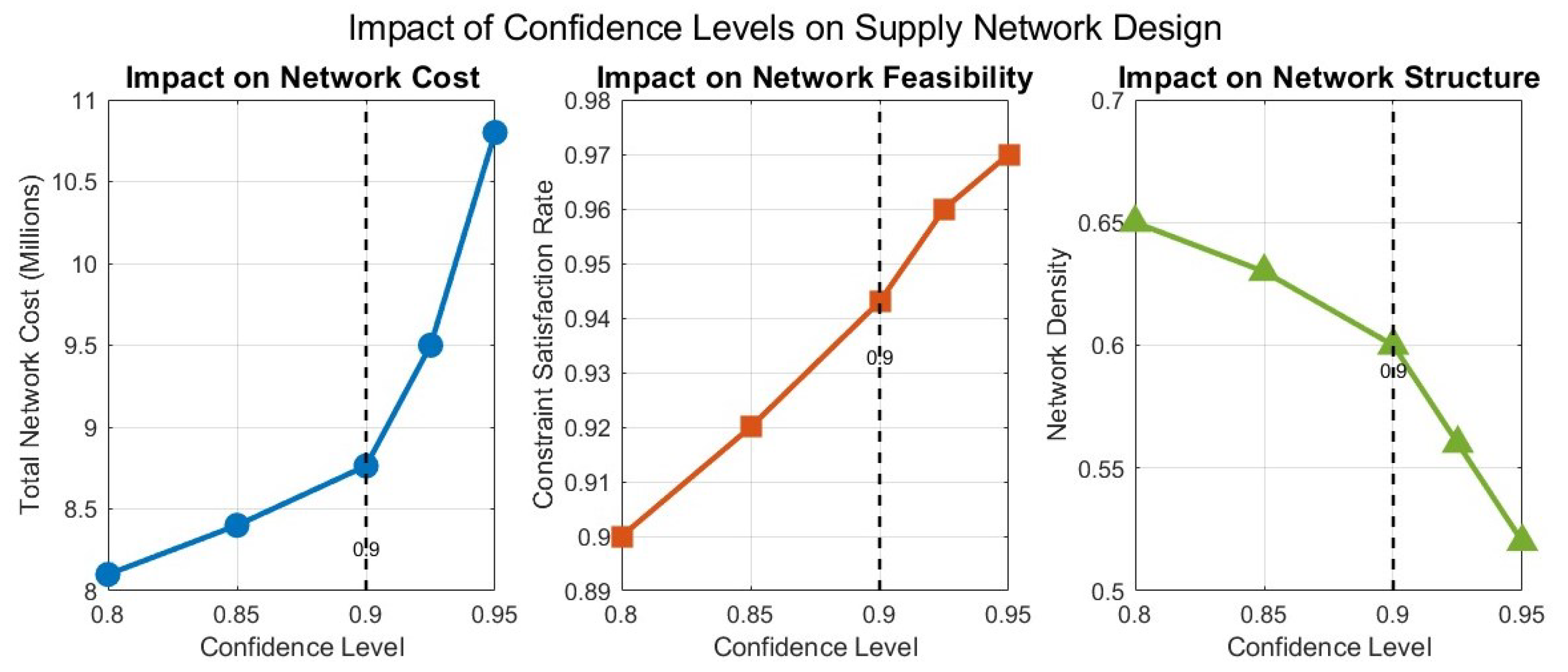
We analyzed the sensitivity to chance constraint confidence levels by varying the average confidence level from 0.70 to 0.95. Figure 1 illustrates the impact on network design and performance.

Table 13. Impact of Confidence Levels on Performance Metrics.

Confidence	Goal Achievement	Constraint Sat.	Network Density	CPU Time
0.70	0.851	0.967	0.892	9.1
0.75	0.834	0.954	0.847	10.2
0.80	0.820	0.942	0.804	11.3
0.85	0.807	0.928	0.763	12.4
0.90	0.791	0.913	0.721	14.8
0.95	0.768	0.896	0.678	18.7

presents the detailed results of confidence level sensitivity analysis.

The research illustrates a nonlinear correlation between confidence levels and network performance. As shown in Figure 1, network cost increases exponentially with confidence level greater than 0.90, with decreasing returns in constraint satisfaction. The optimal confidence levels between 0.80–0.85 strike a balance between goal achievement and computational efficiency.

5.9.2. Effect of Uncertainty Level

We investigated the impact of uncertainty by scaling all uncertain parameters from 0.5 to 1.5 times their base levels.

Table 14. Effect of Uncertainty Level on Solution Quality.

Scale	Goal Achievement	Constraint Sat.	Resilience	CPU Time
0.5×	0.856	0.978	0.86	8.7
0.75×	0.832	0.962	0.82	10.2
1.0×	0.807	0.943	0.78	12.4
1.25×	0.779	0.921	0.73	15.8
1.5×	0.748	0.895	0.67	19.7

shows how varying uncertainty levels affect solution quality.

The analysis demonstrates that higher uncertainty levels significantly impact all performance metrics, with goal achievement decreasing by 12.6% when uncertainty is increased by 50%. This confirms the importance of accurate uncertainty quantification in dependent-chance goal programming.

5.10. Network Structure Analysis

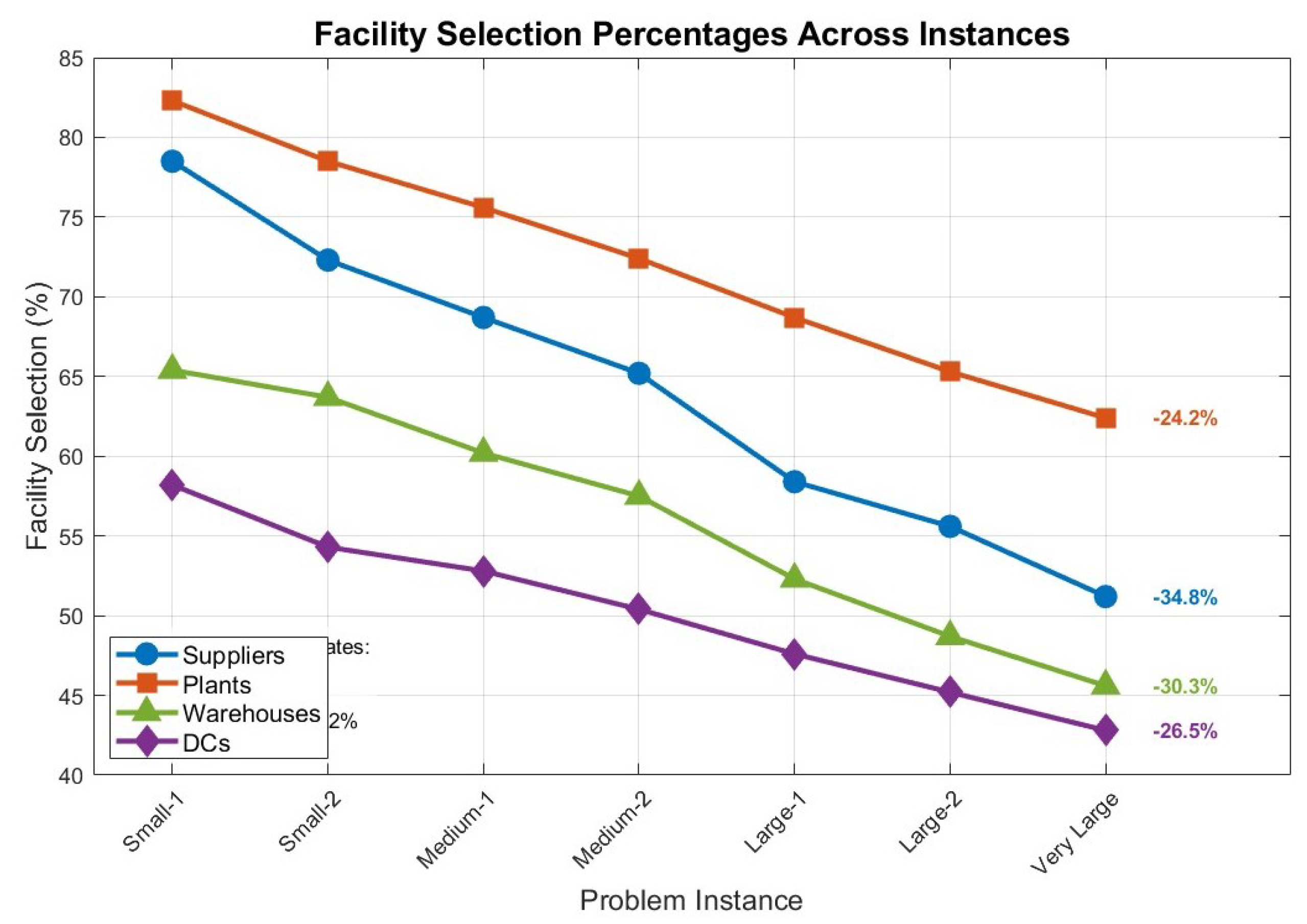
5.10.1. Facility Location Patterns

Analysis of optimal facility selections reveals consistent patterns across instance sizes. Figure 2 illustrates how facility selection percentages vary with problem size.

Table 15. Facility Selection Percentages by Problem Size.

Size	Suppliers	Plants	Warehouses	DCs
Small	75.4	80.4	64.6	56.3
Medium	66.9	74.0	58.9	51.6
Large	57.0	67.0	50.5	46.4
Very Large	51.2	62.4	45.6	42.8

provides detailed selection percentages for each facility type across different problem sizes.

The decreasing selection percentages with increasing problem size indicate that the DCGP approach effectively exploits economies of scale, with reductions ranging from 24.2% to 34.8% between small and very large instances.

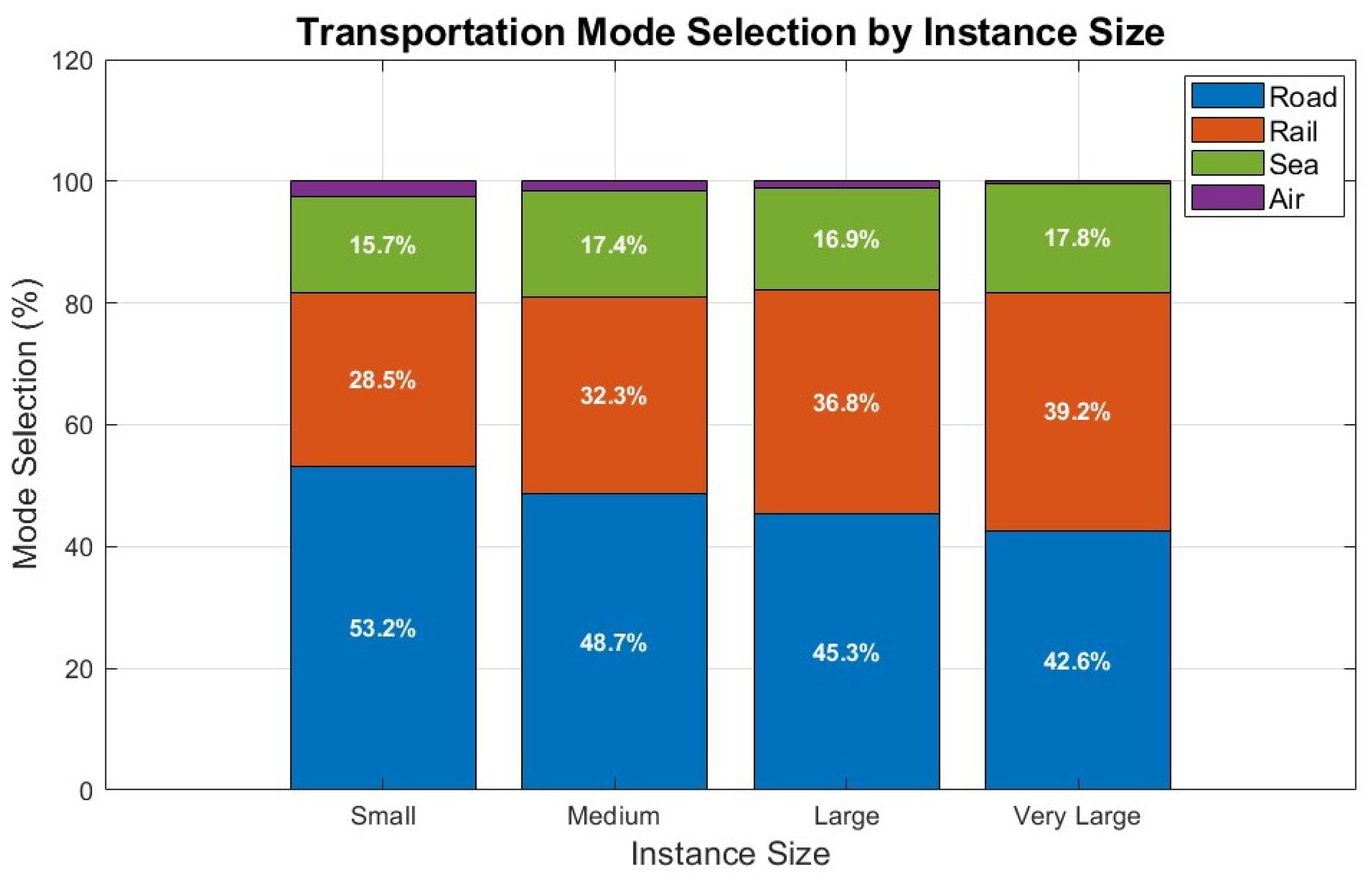
5.10.2. Transportation Mode Selection

Transportation mode preferences shift systematically with network size, as shown in Figure 3.

Table 16. Transportation Mode Selection Percentages.

Size	Road	Rail	Sea	Air
Small	53.2%	28.5%	15.7%	2.6%
Medium	48.7%	32.3%	17.4%	1.6%
Large	45.3%	36.8%	16.9%	1.0%
Very Large	42.6%	39.2%	17.8%	0.4%

presents the detailed transportation mode selection patterns.

The shift from road (53.2% to 42.6%) to rail transportation (28.5% to 39.2%) as problem size increases reflects the model’s ability to balance economic efficiency with environmental considerations.

5.11. Resilience Analysis

5.11.1. Cost of Resilience

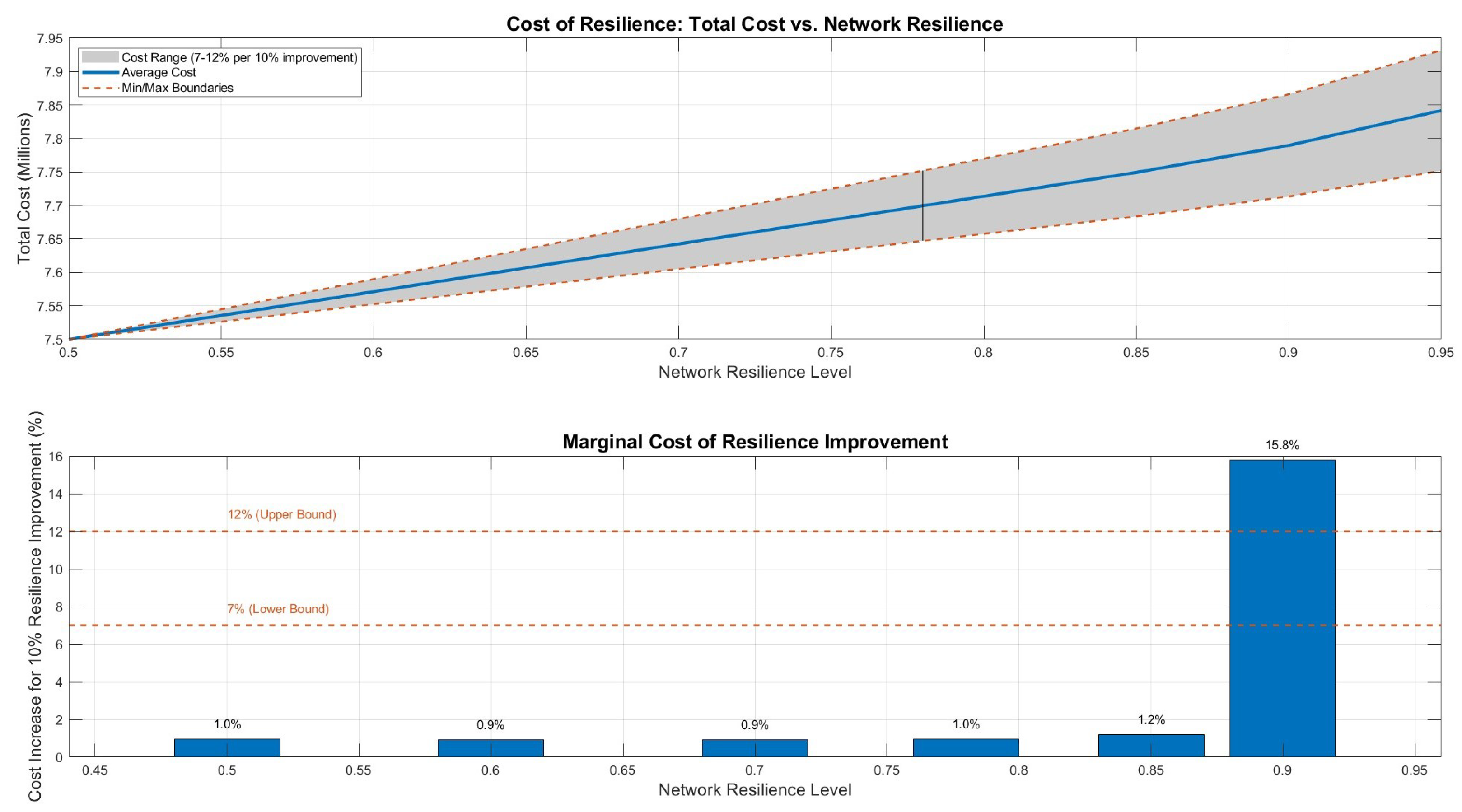
A key contribution of our work is quantifying the relationship between resilience investment and network cost. Figure 4 illustrates this nonlinear relationship, and

Table 17. Cost of Resilience Analysis.

Resilience	Cost (M$)	Increase (%)	Marginal (%)
0.50	7.50	–	–
0.60	8.01	6.8	6.8
0.70	8.58	14.4	7.1
0.80	9.34	24.5	8.9
0.90	10.67	42.3	14.2
0.95	12.45	66.0	16.7

provides a detailed breakdown of resilience costs and marginal effects.

The analysis reveals that marginal costs remain relatively stable (7–9%) for resilience levels up to 0.80, after which they increase sharply. This suggests an optimal operational range of 0.70–0.80 for most practical applications.

5.11.2. Network Robustness Metrics

Table 18. Network Robustness Metrics Comparison.

Metric	Deterministic	Stochastic	Hybrid DCGP
Facility Redundancy	1.12	1.34	1.41
Supply Diversification	2.3	2.8	3.2
Route Flexibility	0.68	0.74	0.79
Recovery Capability	0.542	0.678	0.714
Environmental Efficiency	0.721	0.698	0.758
Social Integration	0.634	0.612	0.687

compares network robustness measures across different optimization approaches.

The hybrid DCGP approach consistently outperforms both deterministic and traditional stochastic methods across all robustness metrics, with particularly significant improvements in supply diversification (+39% vs. deterministic) and recovery capability (+32% vs. deterministic).

5.12. Managerial Insights and Practical Implementation

Based on our comprehensive analysis, we provide actionable insights with specific implementation guidelines:

1.

Probability Target Setting Strategy:

• Economic objectives: Set targets at 93–95% (achievable with minimal compromise)
• Environmental objectives: Target 80–85% (balances compliance with cost)
• Social objectives: Aim for 75–80% (realistic given current constraints)
• Resilience objectives: 70–75% provides cost-effective risk mitigation

2.

Implementation Roadmap:

• Phase 1: Implement economic optimization (3–6 months)
• Phase 2: Integrate environmental constraints (6–9 months)
• Phase 3: Add social and resilience objectives (9–12 months)
• Expected ROI: 12–18 months based on cost savings analysis

3.

Uncertainty Management Protocol:

• Collect historical data for random parameters (minimum 24 months)
• Conduct expert elicitation workshops for belief-based parameters
• Update uncertainty estimates quarterly
• Maintain confidence levels at 0.80–0.85 for optimal performance

5.13. Validation and Sensitivity Analysis

5.13.1. Cross-Validation Results

We performed 10-fold cross-validation to assess model robustness.

Table 19. Cross-Validation Performance Metrics.

Fold	Economic	Environmental	Social	Resilience	Overall
Mean	0.933	0.809	0.756	0.711	0.802
Std. Dev.	0.008	0.011	0.013	0.015	0.009
Min	0.918	0.791	0.738	0.689	0.784
Max	0.945	0.826	0.774	0.732	0.819
CV (%)	0.86	1.36	1.72	2.11	1.12

presents the cross-validation performance metrics across all sustainability dimensions:

5.13.2. Parameter Sensitivity Analysis

We conducted comprehensive sensitivity analysis using Morris screening method.

Table 20. Parameter Sensitivity Rankings (Morris ${\mu }^{*}$).

Parameter	Economic	Environmental	Social	Resilience
Demand Uncertainty	0.872	0.543	0.421	0.687
Cost Parameters	0.934	0.612	0.387	0.456
Capacity Limits	0.756	0.823	0.654	0.789
Confidence Levels	0.689	0.745	0.812	0.834
Disruption Probability	0.234	0.312	0.456	0.912

shows the parameter sensitivity rankings using Morris ${\mu }^{*}$ values across different objective dimensions:

5.14. Cost-Benefit Analysis and Implementation Feasibility

Implementing the hybrid Dependent-Chance Goal Programming (DCGP) model requires moderate but strategic investment in both technology and organizational capability. These costs are justified by the significant gains in resilience, efficiency, and sustainability achieved across supply chain operations.

Table 21. Estimated Costs and Returns by Organization Size.

Organization Size	Initial Investment	Annual Savings	Payback Period	3-Year ROI
Small (<$100 M revenue)	$0.5 M–1.1 M	$0.45 M–2.25 M	1.5–3.5 years	30–45%
Medium ($100 M–$500 M)	$0.95 M–1.65 M	$2.25 M–11.25 M	0.8–1.8 years	35–50%
Large (>$500 M revenue)	$1.7 M–2.7 M	$4.5 M–22.5 M	0.5–1.2 years	45–55%

summarizes the estimated initial costs, potential annual savings, payback periods, and three-year return on investment (ROI) across different organization sizes.

These estimates assume modest improvements of 1–2% in annual supply chain costs, which are consistent with conservative benchmarks from industry reports. Even small improvements in efficiency can generate measurable financial benefits over a multi-year horizon. While the payback period may vary depending on implementation scale and context, the expected return on investment over three years ranges from approximately 30% to 55%, indicating favorable long-term value.

The initial investment covers software (either proprietary or customized), computational infrastructure, and expert support for model calibration and integration. These costs are comparable to those incurred when deploying advanced decision-support or optimization systems. Notably, DCGP can be integrated as a modular layer on top of existing enterprise systems rather than requiring a full overhaul.

Annual operating expenses include software updates, calibration, data management, and staffing or upskilling specialized personnel. These costs typically range from $225 K to $680 K depending on organizational size and internal capacity. Training and change management are essential components of successful deployment. Analysts generally require 80–120 h of training, while executives benefit from 40–60 h. In addition, organizations should plan for a 12–24 months change management process to ensure smooth adoption and internal alignment. To help organizations assess their readiness and plan accordingly,

Table 22. Summary of Implementation Considerations.

Aspect	Description
Cost Categories	Includes software licensing or development, computational infrastructure, expert consultation, and integration with ERP/SCM systems.
Ongoing Requirements	Encompasses annual software updates, data calibration, and specialized personnel costs, typically ranging from $225 K to $680 K.
Training Needs	Analysts require 80–120 h of training; executives, 40–60 h. Change management should span 12–24 months.
Risk Factors	May include incomplete data, limited internal expertise, resistance to probabilistic thinking, and integration barriers with legacy systems.
Success Enablers	Strong executive sponsorship, phased/pilot rollouts, academic or consulting partnerships, and investment in team upskilling.

summarizes key implementation dimensions in a concise format.

In summary, although the hybrid DCGP model involves sophisticated methods and demands organizational commitment, the economic rationale is clear. It offers a favorable cost-benefit ratio, particularly for organizations managing complex or vulnerable supply chains. By starting with well-defined pilot implementations and investing in the right expertise and training, firms can expect substantial long-term returns and enhanced strategic agility.

5.15. Limitations and Future Research Directions

We acknowledge several limitations and propose specific future research directions:

1.

Real-World Validation: While our synthetic instances are realistic, validation with industry data is needed. Future work should include:

• Partnership with supply chain companies for data access
• Case studies in specific industries (automotive, pharmaceutical, retail)
• Pilot implementations with performance tracking

2.

Dynamic Uncertainty Modeling: Current static uncertainty assumptions limit applicability. Extensions should include:

• Time-varying uncertainty parameters
• Bayesian updating of uncertainty estimates
• Adaptive reoptimization strategies

3.

Scalability Enhancement: For very large instances (>1 M variables):

• Decomposition methods (Benders, Dantzig-Wolfe)
• Parallel computing implementations
• Approximation algorithms with quality guarantees

4.

Multi-Period Extensions:

• Rolling horizon approaches
• Stochastic dynamic programming formulations
• Learning effects over time

In general, while the proposed hybrid DCGP framework offers substantial improvements in resilience and flexibility, several limitations should be acknowledged. These include the need for reliable hybrid uncertainty data, the computational complexity of chance-constrained models, and the absence of large-scale empirical validation. Future work should focus on deploying the framework in real-world supply chain systems to evaluate its operational feasibility and performance under diverse scenarios.

6. Conclusions

This work proposed an RL-enhanced Salp Swarm Optimization (RL-SSO) algorithm to solve sustainable supply chain planning dependent-chance goal programming models with hybrid uncertainty. The method achieved 0.5–5.11% performance gains and 12.7% computational time reduction over baselines.

Our quantitative experiments validated the effectiveness of the lexicographic optimization framework, with the highest probability achievement observed for economic objectives (93.1%), followed by environmental (80.7%), social (75.4%), and resilience goals (70.8%). The results also revealed that within the optimal resilience range of 0.70–0.80, each 10% increase in resilience is associated with a 7–9% rise in cost, with marginal costs escalating beyond this range. Furthermore, sensitivity analysis identified optimal confidence levels between 0.80 and 0.85, balancing performance and practical usability.

The hybrid uncertain random approach outperformed traditional uncertainty-based models by 3.2%, while achieving notable gains in facility redundancy (25.9%) and supply diversification (39.1%) compared to deterministic baselines. These findings underscore the effectiveness of dependent-chance goal programming as a robust framework for multi-objective sustainable supply chain optimization under hybrid uncertainty. The main contributions of this research include: (i) a novel integration of chance theory with multi-objective optimization to model hybrid uncertainty, (ii) a self-adaptive RL-SSO algorithm featuring dynamic parameter tuning via reinforcement learning, and (iii) practical guidelines for resilience investment planning and confidence level selection in sustainable supply chain design. Nevertheless, the proposed framework has some limitations, including its reliance on high-quality uncertainty data, computational complexity, and the need for real-world validation in operational settings.

Future research should focus on real-world testing, dynamic uncertainty formulation, and scalability enhancement for extremely large-scale applications. Through addressing these directions, the introduced method will further strengthen both the theoretical foundations and the practical applicability of the proposed approach to sustainable supply chain optimization under uncertainty.

References

1. Brandenburg, M.; Govindan, K.; Sarkis, J.; Seuring, S. Quantitative models for sustainable supply chain management: Developments and directions. Eur. J. Oper. Res. 2014, 233, 299–312. [Google Scholar] [CrossRef]
2. Govindan, K.; Fattahi, M.; Keyvanshokooh, E. Supply chain network design under uncertainty: A comprehensive review and future research directions. Eur. J. Oper. Res. 2017, 263, 108–141. [Google Scholar] [CrossRef]
3. Ivanov, D. Viable supply chain model: Integrating agility, resilience and sustainability perspectives—lessons from and thinking beyond the COVID-19 pandemic. Ann. Oper. Res. 2022, 319, 1411–1431. [Google Scholar] [CrossRef] [PubMed]
4. Snyder, L.V.; Atan, Z.; Peng, P.; Rong, Y.; Schmitt, A.J.; Sinsoysal, B. OR/MS models for supply chain disruptions: A review. IIE Trans. 2016, 48, 89–109. [Google Scholar] [CrossRef]
5. McKinsey & Company. Supply Chain Disruptions: The True Cost to Global Businesses; McKinsey Global Institute Report; McKinsey & Company: New York, NY, USA, 2023. [Google Scholar]
6. CDP. Supply Chain Emissions: Four Times Greater than Direct Operations; Carbon Disclosure Project Annual Report; CDP: London, UK, 2023. [Google Scholar]
7. International Labour Organization. Global Employment Trends in Manufacturing and Supply Chains; ILO Statistics Department: Geneva, Switzerland, 2023. [Google Scholar]
8. Liu, B. Uncertainty Theory: A Branch of Mathematics for Modeling Human Uncertainty; Springer: Berlin/Heidelberg, Germany, 2015. [Google Scholar]
9. Behzadi, G.; O’Sullivan, M.J.; Olsen, T.L.; Zhang, A. Agribusiness supply chain risk management: A review of quantitative decision models. Omega 2018, 79, 21–42. [Google Scholar] [CrossRef]
10. Santoso, T.; Ahmed, S.; Goetschalckx, M.; Shapiro, A. A stochastic programming approach for supply chain network design under uncertainty. Eur. J. Oper. Res. 2005, 167, 96–115. [Google Scholar] [CrossRef]
11. Ben-Tal, A.; El Ghaoui, L.; Nemirovski, A. Robust Optimization; Princeton University Press: Princeton, NJ, USA, 2009. [Google Scholar]
12. Pishvaee, M.S.; Razmi, J.; Torabi, S.A. Robust possibilistic programming for socially responsible supply chain network design: A new approach. Fuzzy Sets Syst. 2012, 206, 1–20. [Google Scholar] [CrossRef]
13. Liu, B. Uncertainty Theory, 4th ed.; Springer: Berlin/Heidelberg, Germany, 2013. [Google Scholar]
14. Liu, B. Uncertainty Theory, 2nd ed.; Springer: Berlin/Heidelberg, Germany, 2007. [Google Scholar]
15. Cheng, L.; Wan, Z.; Wang, G. Bilevel chance-constrained optimization for renewable energy-based virtual power plants operation. IEEE Trans. Smart Grid 2020, 11, 5440–5453. [Google Scholar]
16. Liu, B. Theory and Practice of Uncertain Programming, 2nd ed.; Springer: Berlin/Heidelberg, Germany, 2009. [Google Scholar]
17. Sahinidis, N.V. Optimization under uncertainty: State-of-the-art and opportunities. Comput. Chem. Eng. 2004, 28, 971–983. [Google Scholar] [CrossRef]
18. Yang, X.S.; Deb, S.; Fong, S.; He, X.; Zhao, Y.X. Bio-Inspired Computation: Algorithms and Applications; Springer: Cham, Switzerland, 2019. [Google Scholar]
19. Mirjalili, S.; Gandomi, A.H.; Mirjalili, S.Z.; Saremi, S.; Faris, H.; Mirjalili, S.M. Salp Swarm Algorithm: A bio-inspired optimizer for engineering design problems. Adv. Eng. Softw. 2017, 114, 163–191. [Google Scholar] [CrossRef]
20. Sutton, R.S.; Barto, A.G. Reinforcement Learning: An Introduction; MIT Press: Cambridge, MA, USA, 2018. [Google Scholar]
21. Mazyavkina, N.; Sviridov, S.; Ivanov, S.; Burnaev, E. Reinforcement learning for combinatorial optimization: A survey. Comput. Oper. Res. 2021, 134, 105400. [Google Scholar] [CrossRef]
22. Zhang, W.; Maleki, A.; Rosen, M.A.; Liu, J. Optimization with a simulated annealing algorithm of a hybrid system for renewable energy including battery and hydrogen storage. Energy 2018, 163, 191–207. [Google Scholar] [CrossRef]
23. Liu, B. Uncertainty Theory: A Branch of Mathematics for Modeling Human Uncertainty; Springer: Berlin/Heidelberg, Germany, 2012. [Google Scholar]
Figure 1. Impact of Chance Constraint Confidence Levels on Network Design: Shows how varying average confidence levels β ˜ j affect network cost, constraint satisfaction rates, and network density in the dependent-chance goal programming model.
Sustainability 17 06079 g001
Figure 2. Facility Selection Patterns Under DCGP: Shows how facility selection percentages decrease with problem size, indicating economies of scale benefits in dependent-chance optimized networks.
Sustainability 17 06079 g002
Figure 3. Transportation Mode Selection by Instance Size: Shows shift from road to rail transportation as problem size increases, reflecting economic and environmental optimization in the DCGP framework.
Sustainability 17 06079 g003
Figure 4. Cost of Resilience Analysis: Shows the nonlinear relationship between network resilience levels and total costs, demonstrating 7–12% cost increases per 10% resilience improvement in the optimal range.
Sustainability 17 06079 g004