Assessing and Projecting Long-Term Trends in Global Environmental Air Quality

Abstract

Air quality and environmental issues have gained attention from countries and organizations worldwide over the past several decades. In recent years, carbon peak and carbon neutrality have been mentioned at many international conferences and meetings aimed at reducing and controlling environmental challenges. This study focuses on trend analysis and expectations for the duration of control for environmental air quality (EAQ) indicators, assesses the current EAQ conditions across global countries, and presents reasonable suggestions for environmental control. The study begins by examining the annual, per capita, and per square meter (${\mathrm{m}}^2$) carbon dioxide (CO₂) emission peak and standardizations, where carbon standardization is a replacement for carbon neutrality. A similar quantitative methodology was employed to assess classical air quality factors such as sulfur dioxide (SO₂) and nitrogen oxides (NO_x). The findings suggest that the average control year length (ACYL) of NO_x is longer than that of SO₂, and the ACYL of SO₂ is, in turn, longer than that of CO₂. From an energy structure perspective, regressions results indicate that biofuel and wind power contribute to improvements in EAQ, while coal, oil, and gas power exert negative impacts. Moreover, a long-term EAQ model utilizing an adjusted max–min normalization method is proposed to integrate various EAQ indicators. This study also presents an EAQ ranking for global countries and recommends countries with critical EAQ challenges. The results demonstrate that it is plausible to control EAQ factors at an excellent level with advances in control technologies and effective measures by government, industries, and individuals.

1. Introduction

EAQ is defined based on general air quality (AQ) and takes into account the impact of excessive emissions of greenhouse gases. An excellent EAQ significantly impacts daily life, the national image, and human development. EAQ varies across countries and times at different development levels. Poor EAQ endangers both the physical and mental health of a country’s residents. Furthermore, such countries may decrease the EAQ of the earth if they do not take effective measures to control their EAQ, such as the acid rain problem from the 19th century to the present [1,2], the smog from the 20th century to the present [1,3], and global warming [4,5,6]. Therefore, it is vital to assess the average duration of EAQ control globally across countries, summarize the control experiences of countries with excellent EAQ, and provide suggestions to those facing significant EAQ challenges.

Freeman [7] discusses how the net benefit of environmental policies for a country in the past is useless, but there is value in understanding how to change measures to improve the current net benefit. The EAQ in each country is influenced by industrialization and modernization processes. In retrospect, in countries where EAQ has been historically strongly controlled, it can return to an excellent level with substantial effort. Various organizations and countries have developed air quality standards. However, their estimation models are similar when the max–min normalization method is used [8,9]. The United States Environmental Protection Agency (EPA) introduced the Air Quality Index (AQI) in 1999, which includes factors such as particulate material 2.5 (PM_2.5), ozone, SO₂, carbon monoxide (CO), and nitrogen dioxide (NO₂). A revised AQI shows that the ratio of PM_2.5 to PM₁₀ is greater in southern cities of Taiwan Province, China, than in central or northern cities [10]. Other countries, such as mainland China, Europe, the United Kingdom, and Canada, have established AQIs. Modern monitoring technologies have made it easier to access EAQ factors [9]. Li et al. [11] transfer the concentrations of SO₂, NO_x, and PM₁₀ to air quality indices via the max–min normalization method, using the proportion of the air quality sub-indices SO₂, NO_x, and PM₁₀ in the total index as their initial weights. However, the observations years in Li et al. [11] span from 2016 to 2020, which are insufficient for inferring long-term trends in air quality indicators. This study focuses on long-term EAQ trends, which are challenging to obtain for insufficient monitoring systems.

The Kaya model [12] effectively illustrates carbon emission processes. However, the model focuses on carbon emission flow rather than emission stock [13,14]. The Kaya model also cannot directly depict the changes in carbon emissions over time. Additional studies [12,15] employ the environmental Kuznets curve (EKC) to assess the impact of carbon emissions on economic development, and the results reject the assumption of the significant relationship between carbon emissions and economics. Ru et al. [16] investigate potential EKC relationships between per capita income and EAQ factors such as SO₂, CO₂, and black carbon. With respect to the assessment and perspective of the EAQ, Andres et al. [17] shows that the trends between per capita CO₂ and income levels in developing countries would have a similar “inverted U” path that developed countries have gone through. Lanne and Liski [18] highlight that historical emission trends of per capita CO₂ by fossil fuel combustion began to decline in the 1970s based on the data of early developed countries from 1870 to 1998. Zhong et al. [19] show that emissions activity is the predominant source of global annual SO₂ increase, with the percentage of SO₂ emissions in developing countries at present being greater than that in developed countries in the 1960s. Huang et al. [20] illustrate significant disparities among annual and per capita NO_x emission and its emission intensities, and report that per capita emissions follow an inverted U-shaped EKC. While these articles specifically discuss the relationship between the EAQ factor and time or income levels, none provide a comprehensive long-term trend analysis or assessment. This study primarily focuses on long-term trend analyses and assessments of EAQ indicators.

In this study, three key EAQ factors are considered: CO₂ emissions from fossil fuel combustion, SO₂ emissions from coal and oil combustion in residential heating, and NO_x emissions from vehicles and industrial activities [21,22]. These elements are the primary sources of greenhouse effects, acid rain, and ground-level ozone, respectively. SO₂ and NO_x are the primary air pollutants, and the excessive emission of greenhouse gases such as CO₂ may damage the global environment [4,5,6]. Numerous studies discuss carbon peak and carbon neutrality [23,24]. Many countries, especially developed countries, have already reached their carbon emission peak, while many provide pledges and schedules for carbon neutrality [15,25,26]. Liu et al. [27] argue that provinces such as Guangdong, Zhejiang, and Jiangsu may achieve a carbon peak before 2030, potentially ahead of China’s national commitments, whereas other provinces may lag. Yang et al. [15] also present an evaluation index system of carbon peak and carbon neutrality across Chinese provinces, indicating that provinces with higher scores may more readily achieve these targets. The reasons that other air factors are not suitable for analyzing and estimating EAQ are as follows: the air pollutant CO is excluded from the analysis due to its strong correlation with SO₂ and NO_x. Particulate matter (PM_2.5 and PM₁₀) can be formed secondarily from SO₂ and NO_x and is also omitted [28,29]. Ozone, a secondary pollutant primarily generated through photochemical reaction with NO_x, is likewise excluded [30,31]. Moreover, nitrogen monoxide (NO) and NO₂, the two principal components of NOx, are produced in the gas of vehicles and the combustion of fossil fuels [21,22]. Given that NO is readily transformed to NO2 by chemical reactions with ozone in the air, NOx serves as the reasonable and representative factor for assessing EAQ.

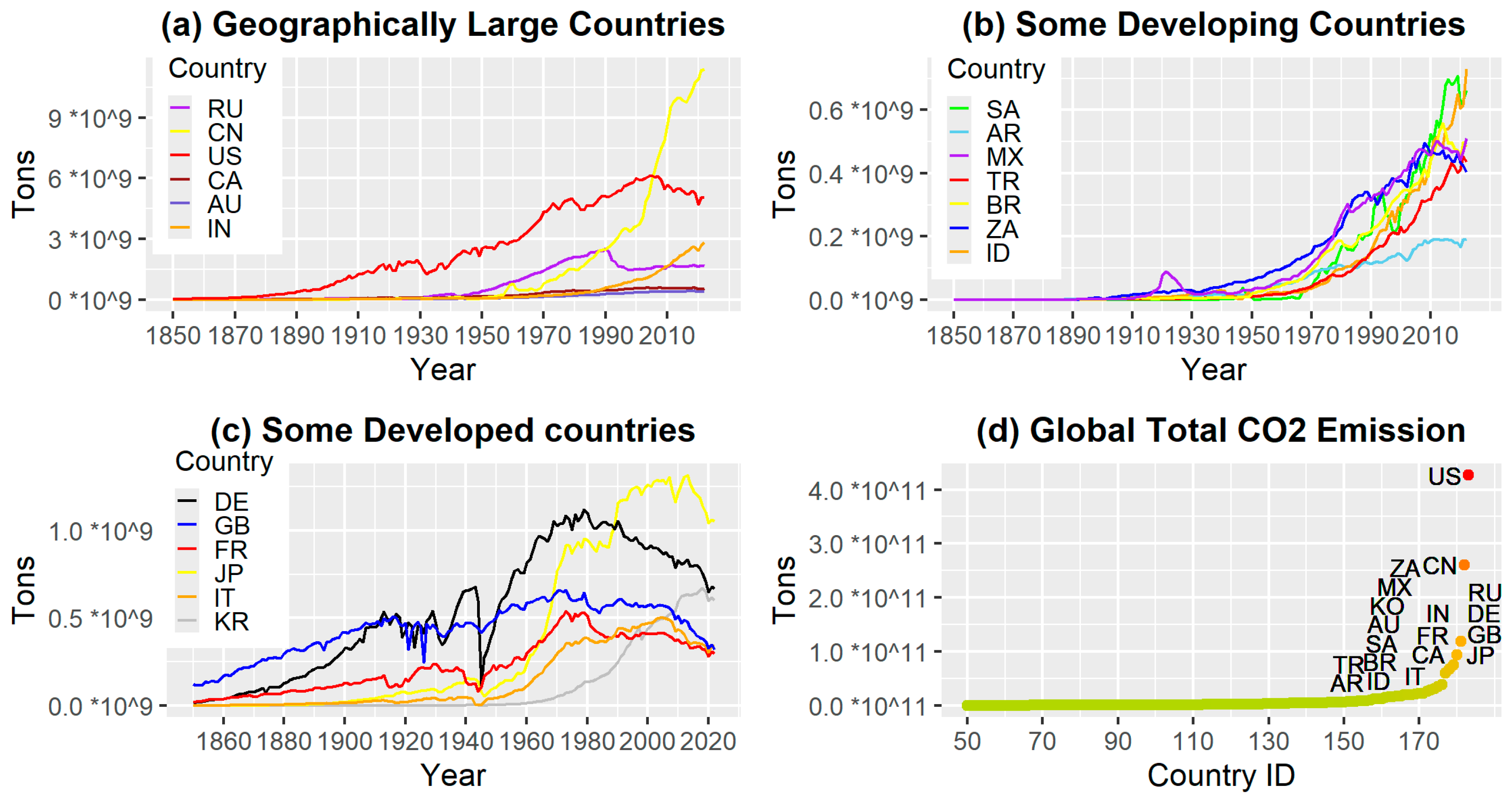
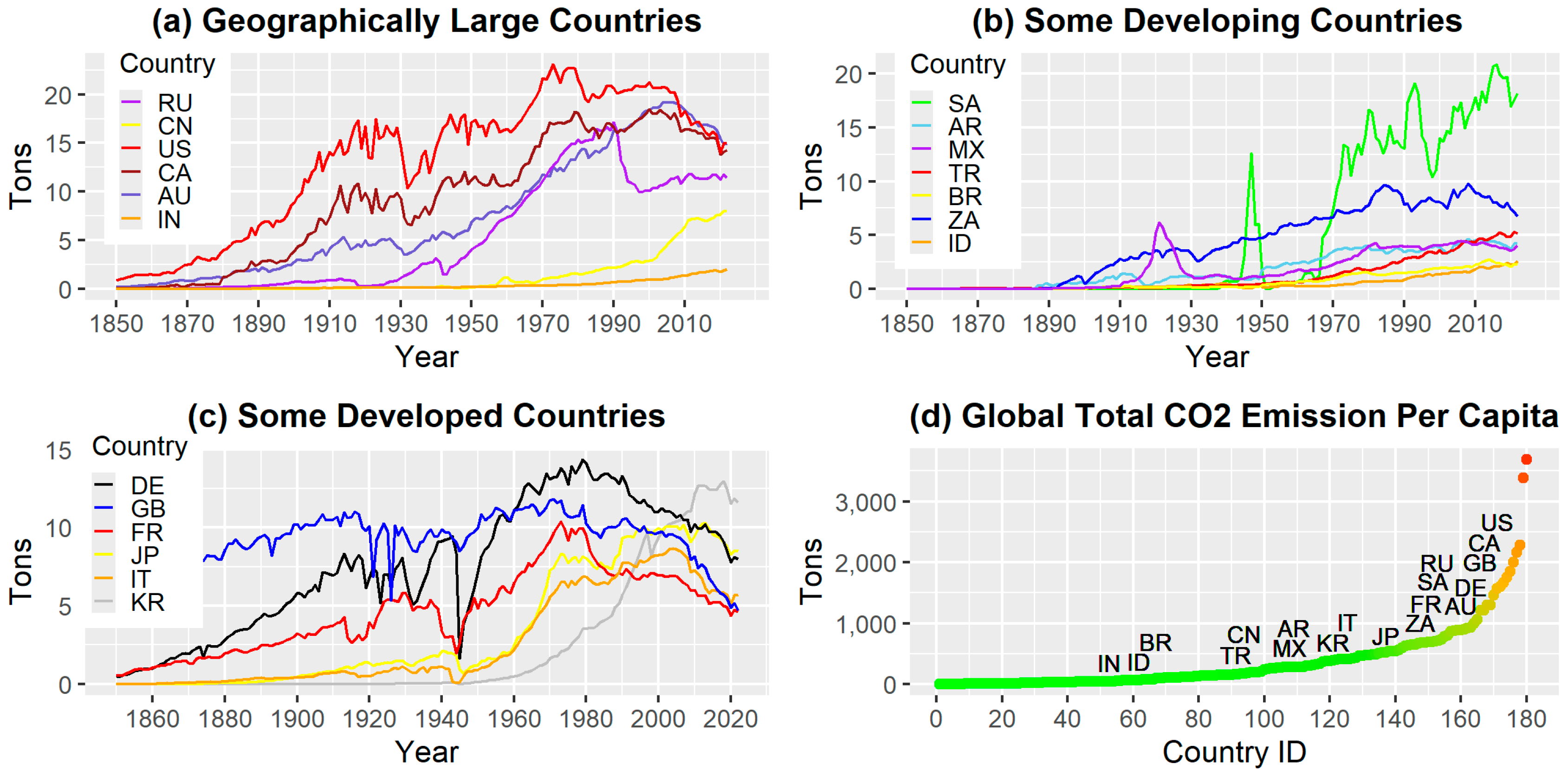
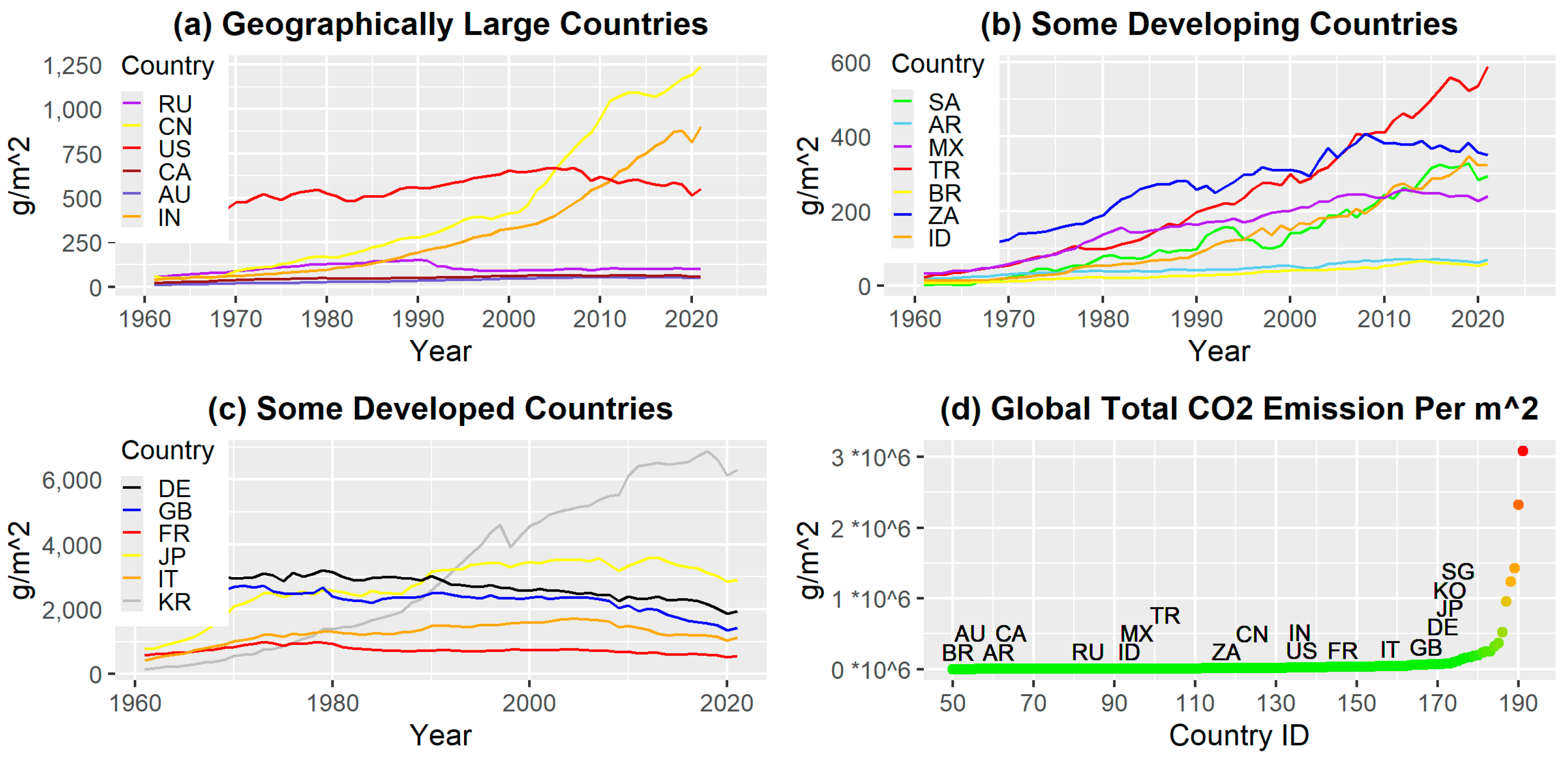
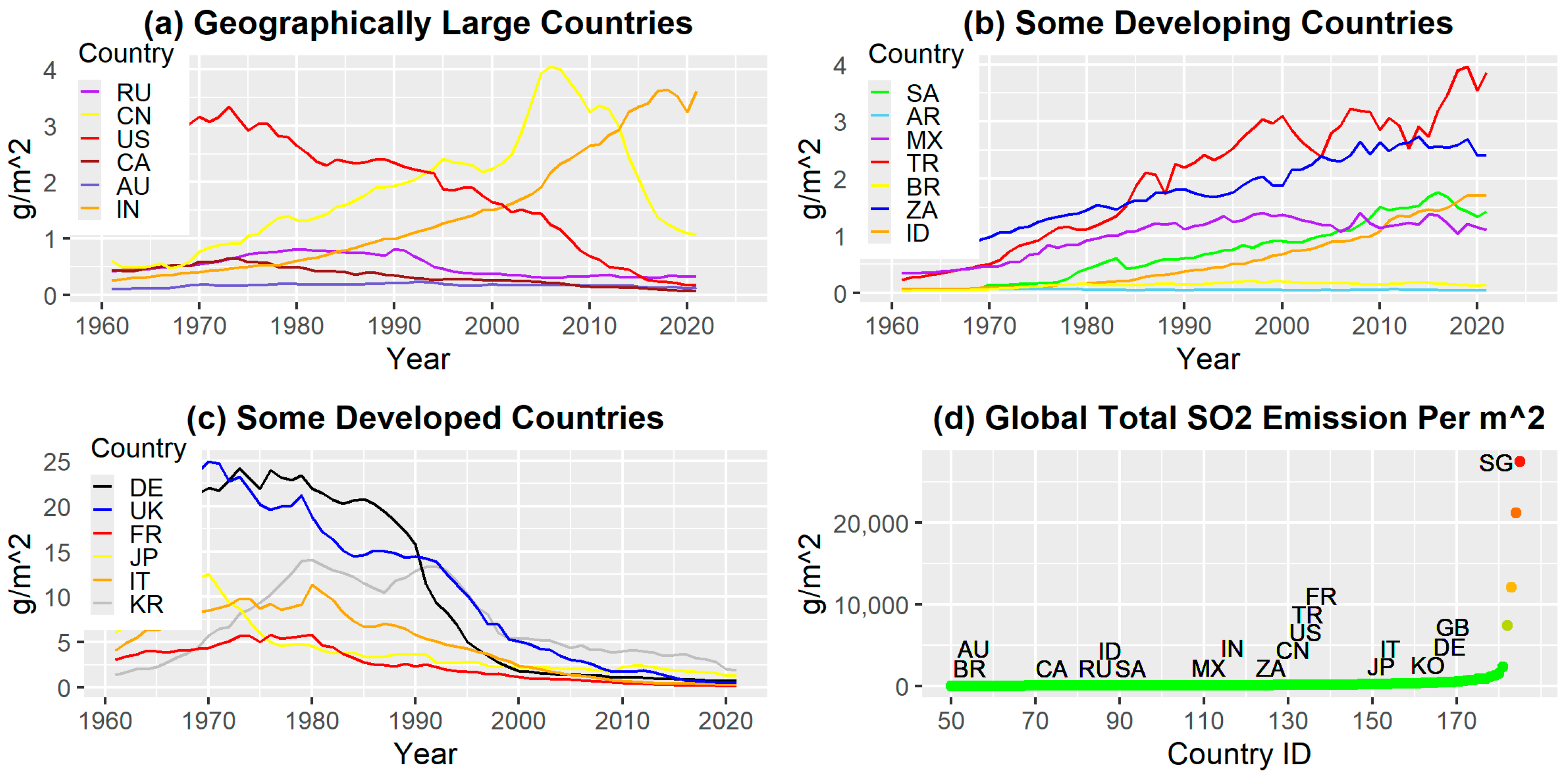
The significance of this study is as follows. First, the impact of CO₂ emissions on the EAQ was examined, along with the assessment of classical air quality factors such as SO₂ and NO_x, which are measured similarly to CO₂. Given the differences in population size and geographic area among countries, considering only the annual emissions of these three factors would lead to bias in analysis and assessment. Therefore, emissions per capita and per ${\mathrm{m}}^2$ are integrated with annual emissions for these three factors to comprehensively evaluate the long-term EAQ of global countries. In addition, some emission rebounds that occur after emission standardization in some countries are given. Second, a regression analysis of the EAQ is conducted from an energy structure perspective. Third, an EAQ ranking model, along with its validation of robustness for global countries, is presented. The primary works of this research include estimating the average duration of EAQ control, assessing the EAQ among various countries, establishing an EAQ ranking model for global countries, summarizing the control strategies of countries with excellent EAQ, and advising countries with critical EAQ challenges.

The remainder of the paper is structured as follows. Section 1 shows the introduction and literature review of the research. Section 2 through Section 4 are structured as three integral components. Section 2 constitutes the first part, in which the key indicators influencing EAQ are identified and described. Section 3 serves as the second part, analyzing the impact of these air quality factors on EAQ. The third part, presented in Section 4, provides a global assessment of EAQ ranking scores and discusses strategies to address associated challenges. Section 5 concludes this study.

2. Long-Term Trend of EAQ

2.1. Histories of EAQ Control and Improvement

Here, historical changes in EAQ control policies across different countries are given to identify existing challenges in EAQ and propose potential solutions. Countries such as Germany, France, Italy, the United Kingdom, Japan, the United States, and China have implemented effective strategies for improving EAQ, although the value of some EAQ indicators is still high in China and the United States. In Europe, representative countries such as Germany, France, and Italy have adopted several measures to reduce the anthropogenic emissions of EAQ factors [32].

Spix et al. [33] and Popp [34] report that East Germany established strict air emission standards in the 1980s, and the former West Germany adopted these standards in the 1990s after unification. The United Kingdom established the Clean Air Act in 1968, followed by the Control of Pollution Act in 1974. Similarly, Japan enacted the Air Pollution Control Law in 1968, which has since been amended twice [32]. In the United States, the Environmental Protection Agency (EPA) was established, and the Clean Air Act was implemented in 1970 and later amended in 1990 [7,34].

In 1998, China enacted the Atmospheric Pollution Prevention and Control Law of the People’s Republic of China, which has since undergone several amendments. In 2013, China implemented the Action Plan on Prevention and Control of Air Pollution and the Three-Year Plan of Action for Winning the War to Protect Blue Skies in 2018. Barwick et al. [35] report that China launched air quality monitoring programs and disclosed air quality information nationwide, given the lack of transparency on air quality and the unawareness of excessive emissions of EAQ factors before 2013. These initiatives indirectly and significantly decreased the mortality associated with air pollution in the years after 2013.

Unlike countries making high-magnitude improvements to EAQ, India continues to face significant challenges related to EAQ. The number of smog days is high in many Indian cities. Although India enacted the Air (Prevention and Control of Pollution) Act in 1981, amended it multiple times, and launched the National Clean Air Programme in 2019, these efforts have not sufficiently addressed the air pollution issues.

2.2. Assumptions and Data Sources

The assumptions of this research are as follows: The first assumption is that emissions from industrialization, modernization, and residential heating are considered the main sources affecting the EAQ of global countries. The second assumption limits the possibility that there are no spillover effects of the EAQ between countries. The third assumption requires that each level of EAQ indicators becomes consistent across all countries once their EAQ indicators reach emission standards, considering the emission quantities of EAQ indicators.

The data sources for this study include the Global Carbon Budget (GCB) (2023) [36] and the Community Emissions Data System (CEDS) 2024 [37], both curated and disseminated by Our World in Data. For validation purposes, the annual emissions data for the United States from 1990 to 2022 show a high level of consistency among the four data sources—Our World in Data, the United States EPA, the Emissions Database for Global Atmospheric Research (EDGAR) [38], and the World Bank—with Pearson correlation coefficients all exceeding 0.97. At the global level, the significant percentages of countries with CO₂, SO₂, and NO_x emissions are all above 0.77, and the correlations of these factors’ annual emissions from 1970 to 2022 between Our World in Data and the EDGAR are all above 0.7. Some countries with more than two lower correlations for CO₂, SO₂, and NO_x between Our World in Data and the EDGAR are excluded from the remainder of the analysis. This is reasonable for biases within data on emissions per capita and per ${\mathrm{m}}^2$ because these data rely on the population and geographical area of global countries from different data sources. Overall, the data used in this study are derived primarily from GCB 2023 and CEDS 2024, as curated and disseminated by Our World in Data. The detailed data can also be found in the Supplementary Materials.

2.3. Emission Peak and Standardization of EAQ Indicators

As mentioned in the Introduction, fewer than 60 countries have reached their carbon peak, and an even smaller number have achieved carbon neutrality [15,25,26]. Even countries with well-controlled EAQ factors, such as France, Japan, Germany, Italy, and the United Kingdom, have pledged to achieve net-zero carbon emissions by the middle of the 21st century [39]. In this subsection, the concepts of carbon peak and neutrality are expanded by applying them to annual, per capita, and per ${\mathrm{m}}^2$ CO₂ peak and standardization. Carbon standardization replaces carbon neutrality due to the lack of sample countries that have reached carbon neutrality. Moreover, classical air quality factors such as SO₂ and NO_x are analyzed in similar ways as CO₂, where both SO₂ and NO_x have an annual, per capita, and per ${\mathrm{m}}^2$ emission peak and standardization.

Emissions standardization is defined as emission target achievement (ETA) when the emission of each EAQ indicator decreases to $\phi$ of the largest percentage of the emission value at present divided by its peak among all countries. Emissions standardization is defined as emission target achievement (ETA), whereby the emission of each EAQ indicator is reduced to a proportion $\phi$ of the largest percentage of the emission value at present divided by its historical peak across all countries. Here, ${\phi }_j\in (0, 1]$ represents the predefined threshold and $j\in \left\{\mathrm{1,2},\dots ,9\right\}$ denotes EAQ indicators. The definition of emissions standardization implies that each EAQ indicator is associated with an actual ETA value, denoted as ${\widehat{\phi }}_j$, which corresponds to ${\phi }_j$ times the largest percentage of the emission value at present divided by its historical peak across all countries.

Table A1. Standardization thresholds of EAQ indicators ${\mathrm{P}\mathrm{C}\mathrm{E}}_{y^{ETA}}$.

${\mathit{\phi }}_{\mathit{j}}$	${\widehat{\mathit{\phi }}}_{\mathit{j}}$	${\mathit{\phi }}_{\mathit{j}}$	${\widehat{\mathit{\phi }}}_{\mathit{j}}$	${\mathit{\phi }}_{\mathit{j}}$	${\widehat{\mathit{\phi }}}_{\mathit{j}}$
$\mathit{j}\in \left\{\mathrm{1,2},3\right\}$		$\mathit{j}\in \left\{\mathrm{4,5},6\right\}$		$\mathit{j}\in \left\{\mathrm{7,8},9\right\}$
CO2		PCO2		PSMCO2
0.6	0.54	0.6	0.59	0.7	0.70
SO2		PSO2		PSMSO2
0.8	0.80	0.8	0.8	0.8	0.8
NOx		PNOx		PSMNOx
0.7	0.65	0.7	0.69	0.8	0.8

Note: PCO₂, PSO₂, and PNO_x represent per capita CO₂, SO₂, and NO_x emissions, respectively. PSMCO₂, PSMSO₂, and PSMNO_x represent per ${\mathrm{m}}^2$ CO₂, SO₂, and NO_x emissions, respectively. The standardization thresholds ${\phi }_j$ that are set at or below 50% are overly inclusive, while those set at or above 90% are excessively restrictive. Therefore, these extreme values are excluded from the analysis. For total CO₂ and CO₂ per capita emissions, thresholds ${\phi }_j$ of 0.7 or 0.8 result in the exclusion of several countries, including France and Germany, suggesting that these values are too stringent. Consequently, a threshold of ${\phi }_j=0.6$ is adopted for these two indicators. For indicators such as NO_x, NO_x per capita, and CO₂ per m², the standardization threshold ${\phi }_j$ is set at 0.7. This value represents a balance: when ${\phi }_j=0.6$, a disproportionately large number of countries meet the standard, whereas ${\phi }_j=0.8$ excludes too many. For the remaining indicators—SO₂, SO₂ per capita, NO_x per capita, SO₂ per m², and NO_x per m²—a standardization threshold of ${\phi }_j=0.8$ is employed, as it results in a more reasonable number of countries reaching standardization compared to lower thresholds of 0.6 or 0.7, which are accompanied by a large number of countries. These threshold selections aim to ensure analytical consistency and robustness.

presents the specific thresholds ${\phi }_j$ and the corresponding ${\widehat{\phi }}_j$ for each EAQ indicator. Additionally, a sensitivity analysis is conducted across all nine EAQ indicators, wherein ${\phi }_j$ are set as 0.6, 0.7, and 0.8 to examine the robustness of the results. Further details of the sensitivity test are provided in the accompanying explanation of Table A1.

The nine EAQ indicators of global countries specifically for countries in Group 20 (G20) are discussed in the rest of the research. These EAQ indicators include the annual emissions, emissions per capita, and emissions per ${\mathrm{m}}^2$ of CO₂, SO₂, and NO_x. An examination of the long-term historical trends and average duration of control of these EAQ factors is presented, considering their peak and standardizations. The duration of control is the number of emission control years from the emission peak to its standardization, and the ACYL represents the statistical average from peak to standardization. Each EAQ factor is assessed using six key points, including the emission peak and emission standardizations on an annual, per capita, and per ${\mathrm{m}}^2$ basis. Furthermore, $E_{i,j,y}$ represents the emissions of the $j$-th indicator for country $i$ in year $y$. $i$ is the country number organized alphabetically, $j$ represents the EAQ indicator and can be a value from $\left\{\mathrm{1,2},\cdots ,9\right\}$, and $y$ belongs to the set of observation years. Let $y_{i,j}^{peak}=\left(y:\underset{y}{\max }\left\{E_{i,j,y}\right\}\right)$ be the year when the emissions of the $j$-th indicator in country $i$ reach their peak level. Let $y_{i,j}^{ETA}$ represent the year when the emissions reach the emission standardization threshold for the $j$-th indicator in country $i$. The pollution control effect (PCE) is calculated using max–min normalization for the $j$-th indicator in country $i$ and year $y$, where the PCE is expressed as follows:

$${\mathrm{P}\mathrm{C}\mathrm{E}}_{i,j,y}={\displaystyle \frac{\underset{y}{\max }\left\{E_{i,j,y}\right\}-E_{i,j,y}}{\underset{y}{\max }\left\{E_{i,j,y}\right\}-\underset{y}{\min }\left\{E_{i,j,y}\right\}}},$$

(1)

Equation (1) indicates that ${\mathrm{P}\mathrm{C}\mathrm{E}}_{i,j,y^{peak}}=0$, where $y^{peak}$ represents the peak year; ${\mathrm{P}\mathrm{C}\mathrm{E}}_{i,j,y^{max}}$ is the PCE in the latest year, where $y^{max}$ is the latest year observed; and ${\mathrm{P}\mathrm{C}\mathrm{E}}_{·,j,y^{ETA}}$ is 60% of the largest ratio of the emission of the EAQ indicator $j$ at present divided by its emission peak. ${\mathrm{P}\mathrm{C}\mathrm{E}}_{·,j,y^{ETA}}$ signifies the threshold where the emission of the EAQ indicator meets the standardization criteria, which are outlined in Table A1. Each EAQ indicator’s PCE is categorized into three distinct intervals. The first interval, [0, 0.05], shows indicators that have not reached the emission peak. In general, significance levels equal to 0 suggests that the indicators have not yet reached their emission peak. However, emission levels may fluctuate around the peak and potentially rise again at a later stage. Therefore, a significance level of 0.05 is adopted to enhance the robustness of the analysis. The second interval, (0.05, ${\mathrm{P}\mathrm{C}\mathrm{E}}_{y^{ETA}}$], shows that indicators have reached the emission peak and that emissions are under preliminary control. The third interval, (${\mathrm{P}\mathrm{C}\mathrm{E}}_{y^{ETA}}$, 1], is where indicators have achieved the emission targets.

2.4. Trend and Expectation of the EAQ Indicators

Figure 1, Figure 2, Figure 3, Figure 4, Figure 5, Figure 6, Figure 7, Figure 8 and Figure 9 illustrate the long-term trends of the EAQ indicators for global countries. In each figure, panels (a) to (c) depict the annual trends of the EAQ indicator for G20 countries, with countries categorized into three groups based on emission levels. Panel (a) includes countries characterized by large geographic areas, such as Russia, China, the United States, Canada, Brazil, Australia, and India. Panel (b) shows a group of some developing countries, including Saudi Arabia, Argentina, Mexico, Turkey, Brazil, South Africa, and Indonesia. Panel (c) comprises some developed countries, such as Germany, the United Kingdom, France, Japan, Italy, and South Korea. These geographic area data and country classification information are obtained from the World Bank and United Nations. Panel (d) in each figure provides a ranking based on the cumulative sum of annual EAQ indicator emissions, where the countries on the right side of the panel exhibit higher total emissions. The specific ranking data for panel (d) in Figure 1, Figure 2, Figure 3, Figure 4, Figure 5, Figure 6, Figure 7, Figure 8 and Figure 9 and the Alpha-2 codes of the countries can be found in the Supplementary Materials.

Table A2. Peak year and current control situation of annual emissions.

Country	${\mathit{y}}_{·,\mathit{j}}^{\mathit{p}\mathit{e}\mathit{a}\mathit{k}},\mathit{j}\in \left\{\mathrm{1,2},3\right\}$ (Year)			${\mathbf{P}\mathbf{C}\mathbf{E}}_{·,\mathit{j},{\mathit{y}}^{\mathit{m}\mathit{a}\mathit{x}}}\mathit{j}\in \left\{\mathrm{1,2},3\right\}$ (%)
Indicator	CO2	SO2	NOx	CO2	SO2	NOx
Argentina	2022	1971	2013	0	0.3844	0.1084
Australia	2019	1993	1996	0.0566	0.4122	0.3488
Brazil	2014	1997	2014	0.1334	0.3893	0.1915
Canada	2007	1973–2001 (28)	1980–2016 (36)	0.0772	0.893	0.5379
China	2022	2006–2017 (11)	2012	0	0.7338	0.3365
France	1973–2014 (41)	1980–1988 (8)	1978–2009 (31)	0.4646	0.9858	0.7140
Germany	1979–2020 (41)	1973–1992 (19)	1986–2009 (23)	0.4101	0.9718	0.7013
Indonesia	2022	2022	2022	0	0	0
India	2022	2022	2018	0	0	0.0484
Italy	2005–2020 (15)	1980–1994 (14)	1992–2009 (17)	0.3270	0.9783	0.6888
Japan	2013	1970–1977 (7)	1975–2005 (30)	0.1987	0.8885	0.7214
KR	2018	1980–1999 (19)	2004	0.1032	0.8655	0.3682
Mexico	2022	2008	2008–2020 (12)	0	0.2308	0.4470
Russia	1990–1997	1980–2005	1990–2009	0.3486	0.6096	0.4303
SA	2019	2016	2015	0.0630	0.1031	0.0112
ZA	2008	2014	2014	0.1840	0.1580	0.2009
Turkey	2021	2019	2007	0.0376	0.0222	0.1949
GB	1971–2014 (43)	1970–1995 (25)	1973–2007 (34)	0.6270	1	0.7914
US	2005	1973–2006 (33)	1979–2009 (30)	0.1759	0.9459	0.6943
ACYL	15.84	22.83	24.92

Note: $y_{·,j}^{peak}$ represents the year when the emissions of the $j$-th indicator reach their peak level. $y_{·,j}^{peak}$ equal to 2022 indicates that the country has not reached the emission peak so far. ${\mathrm{P}\mathrm{C}\mathrm{E}}_{·,j,y^{max}}$ represents the PCE in the latest year, where $y^{max}$ is the latest year observed. The number in the round bracket on the right side of the year peak or year interval is the control year length. The three colors marked in the PCE chart reflect the different degrees of control of the EAQ indicators. Specifically, the red symbols signify countries that have not yet reached the emission peak and fall within [0, 0.05]. The orange symbols indicate that countries reached the emission peak when their emission control was insufficient and that their PCE intervals are (0.05, ${\mathrm{P}\mathrm{C}\mathrm{E}}_{y^{ETA}}$]. The green symbols illustrate that countries reached the emission peak and standardization when their PCEs are beyond ${\mathrm{P}\mathrm{C}\mathrm{E}}_{y^{ETA}}$. Due to the dissolution of the Soviet Union, Russia exhibited irregular emission trends after 1990. As a result, the analysis of Russia’s emission trends has been excluded from this manuscript.

,

Table A3. Peak year and current control situation of per capita emissions.

Country	${\mathit{y}}_{·,\mathit{j}}^{\mathit{p}\mathit{e}\mathit{a}\mathit{k}},\mathit{j}\in \left\{\mathrm{4,5},6\right\}$ (Year)			${\mathbf{P}\mathbf{C}\mathbf{E}}_{·,\mathit{j},{\mathit{y}}^{\mathit{m}\mathit{a}\mathit{x}}}\mathit{j}\in \left\{\mathrm{4,5},6\right\}$ (%)
Indicator	PCO2	PSO2	PNOx	PCO2	PSO2	PNOx
Argentina	2008	1971–2018 (47)	2013	0	0.6878	0.1694
Australia	2004	1971–2015 (44)	1990–2022 (32)	0.2219	0.7298	0.5999
Brazil	2014	1979	2014	0.1811	0.5407	0.2389
Canada	2000	1973–1991 (18)	1980–2014 (34)	0.2293	0.9420	0.7170
China	2022	2006–2016 (10)	2012	0	0.7518	0.3637
France	1973–1994 (21)	1973–1987 (14)	1978–2013 (35)	0.5877	1.0000	0.7776
Germany	1979–2018 (39)	1973–1992 (19)	1986–2018 (32)	0.4579	0.9977	0.7324
Indonesia	2022	2022	2022	0	0	0
India	2022	2017	2018	0	0.0054	0.0841
Italy	2004–2020 (16)	1980–1994 (14)	1992–2013 (21)	0.3394	0.9716	0.7048
Japan	2013	1970–1980 (10)	1973–2009 (36)	0.1747	0.9040	0.7496
KR	2018	1979–2014 (35)	2004	0.1056	0.8098	0.4188
Mexico	2006	1987	1994	0.3462	0.4664	0.5792
Russia	1990	1980–2004	1990	0.3338	0.6308	0.4191
SA	2016	1990	1990	0.1281	0.1903	0.1655
ZA	2008	2008	2008	0.3111	0.3075	0.3327
Turkey	2021	1998	2007	0.0440	0.0677	0.3536
GB	1971–2020 (37)	1970–1995 (25)	1973–2009 (36)	0.6116	1.0000	0.8727
US	1973–2020 (47)	1973–2000 (27)	1973–2009 (36)	0.3656	0.9966	0.8176
ACYL	20.32	24.68	24.92

Note: $y_{·,j}^{peak}$ represents the year when the emissions of the $j$-th indicator reach their peak level. $y_{·,j}^{peak}$ equal to 2022 indicates that the country has not reached the emission peak so far. ${\mathrm{P}\mathrm{C}\mathrm{E}}_{·,j,y^{max}}$ represents the PCE in the latest year, where $y^{max}$ is the latest year observed. The number in the round bracket on the right side of the year peak or year interval is the control year length. The three colors marked in the PCE chart reflect the different degrees of control of the EAQ indicators. Specifically, the red symbols signify countries that have not yet reached the emission peak and fall within [0, 0.05]. The orange symbols indicate that countries reached the emission peak when their emission control was insufficient and that their PCE intervals are (0.05, ${\mathrm{P}\mathrm{C}\mathrm{E}}_{y^{ETA}}$]. The green symbols illustrate that countries reached the emission peak and standardization when their PCEs were ${\mathrm{P}\mathrm{C}\mathrm{E}}_{y^{ETA}}$. The emission per capita trend of SO₂ and NO_x in Saudi Arabia is unusual and increased dramatically in the 1970s. The maximum emission of SO₂ and NO_x in Saudi Arabia was set as the emission value in 1990.

and

Table A4. Peak year and current control situation of per ${\mathit{m}}^2$ emissions.

Country	${\mathit{y}}_{·,\mathit{j}}^{\mathit{p}\mathit{e}\mathit{a}\mathit{k}},\mathit{j}\in \left\{\mathrm{7,8},9\right\}$ (Year)			${\mathbf{P}\mathbf{C}\mathbf{E}}_{·,\mathit{j},{\mathit{y}}^{\mathit{m}\mathit{a}\mathit{x}}}\mathit{j}\in \left\{\mathrm{7,8},9\right\}$ (%)
Indicator	PSMCO2	PSMSO2	PSMNOx	CO2	SO2	NOx
Argentina	2015	1971–1985 (14)	2013	0.0141	0.7899	0.1389
Australia	2019	1993–2015 (22)	1996	0.0889	0.7633	0.5386
Brazil	2014	1997	2014	0.1193	0.3656	0.1650
Canada	2007	1973–1991 (20)	1980–2011 (31)	0.1145	0.9988	0.9244
China	2021	2006–2016 (10)	2012	0	0.8318	0.3313
France	1973–1986 (13)	1980–1988 (8)	1978–2008 (30)	0.9018	1	0.9817
Germany	1979–2007 (40)	1973–1992 (19)	1986–2004 (18)	0.9331	0.9984	0.9905
Indonesia	2019	2019	2019	0.0635	0.0025	0.0151
India	2021	2018	2018	0	0.0036	0.0864
Italy	2005	1980–1994 (14)	1992–2008 (16)	0.4376	1	0.9749
Japan	2013	1970–1976 (6)	1975–2006 (31)	0.2447	0.9957	0.9237
KR	2018	1980–1998 (18)	2004	0.0833	0.9627	0.3851
Mexico	2012	2008	2008	0.0749	0.2846	0.5614
Russia	1990–1995	1980–1994	1990–1997	0.5067	0.9441	0.6378
SA	2019	2016	2015	0.1076	0.1965	0.0819
ZA	2008	2014	2014	0.1769	0.1622	0.2276
Turkey	2021	2019	2007	0	0.0259	0.1822
GB	1971–2011 (28)	1970–1995 (25)	1973–2008 (35)	0.9365	1	0.9972
US	2005	1973–2006 (33)	1979–2009 (30)	0.3366	0.9952	0.9767
ACYL	16.19	20.67	24.56

Note: $y_{·,j}^{peak}$ represents the year when the emissions of the $j$-th indicator reach their peak level. $y_{·,j}^{peak}$ equal to 2022 indicates that the country has not reached the emission peak so far. ${\mathrm{P}\mathrm{C}\mathrm{E}}_{·,j,y^{max}}$ represents the PCE in the latest year, where $y^{max}$ is the latest year observed. The number in the round bracket on the right side of the year peak or year interval is the control year length. The three colors marked in the PCE chart reflect the different degrees of control of the EAQ indicators. Specifically, the red symbols signify countries that have not yet reached the emission peak and fall within [0, 0.05]. The orange symbols indicate that countries reached the emission peak when their emission control was insufficient and that their PCE intervals are (0.05, ${\mathrm{P}\mathrm{C}\mathrm{E}}_{y^{ETA}}$]. The green symbols illustrate that countries reached the emission peak and standardization when their PCEs were ${\mathrm{P}\mathrm{C}\mathrm{E}}_{y^{ETA}}$.

present the emission peak year $y_{i,j}^{peak}$ and the latest ${\mathrm{P}\mathrm{C}\mathrm{E}}_{i,j,y^{max}}$, where $i$ represents the country and $j$ represents the EAQ indicator. In these tables, the emission peak years or emission control intervals from emission peak to standardization are given when countries’ EAQ indicators have reached their emission peak or standardization. The number in the round bracket on the right side of the year peak or year interval is the ACYL. The three colors marked in the PCE chart reflect the different degrees of control of the EAQ indicators. Specifically, the red symbols signify countries that have not yet reached the emission peak and fall within the first interval of the PCE mentioned in Section 2.2. In general, the year 2022 represents a point when a country has not yet reached its emission peak, but a 0.05 significance level is adopted here for robustness purposes. The orange symbols indicate that countries reached the emission peak when their emission control was insufficient and that their PCEs were within the second interval. The green symbols illustrate countries that reached the emission peak and standardization where their PCEs reached the third interval.

Figure 1, Figure 2 and Figure 3 illustrate the historical trends of the three EAQ factors’ annual emissions in G20 countries from 1850 to 2021. Table A2 lists the emission peak year $y_{i,j}^{peak}$ and the latest ${\mathrm{P}\mathrm{C}\mathrm{E}}_{i,j,y^{max}}$, where $i$ represents the country and $j\in \left\{\mathrm{1,2},3\right\}$. $j$ equal to 1, 2, and 3 represent the annual emissions of CO₂, SO₂, and NO_x, respectively. These results indicate that India and Indonesia have not yet reached their annual emission peaks for all three emission indicators. Turkey has two indicators that have not reached the emission peak, whereas another indicator falls within the second interval of the PCE. Only France, Germany, Italy, Japan, and the United States have not reached the standardization of total CO₂ emission. The United Kingdom has successfully reached all thresholds of total emissions standardization. Furthermore, the average control year lengths of the annual emissions of CO₂, SO₂, and NO_x are 15.84, 22.83, and 24.92, respectively, among global countries. Specific information on the ACYL of global countries can be found in the Supplementary Materials.

Figure 4, Figure 5 and Figure 6 depict the historical trends of the three EAQ factors’ per capita emissions for G20 countries from 1850 to 2021. Table A3 shows the per capita emission peak year $y_{i,j}^{peak}$ and the latest ${\mathrm{P}\mathrm{C}\mathrm{E}}_{i,j,y^{max}}$, where $i$ represents the country and $j\in \left\{4, 5, 6\right\}$. $j$ equal to 4, 5, and 6 represent the emissions per capita of CO₂, SO₂, and NO_x, respectively. These results demonstrate that Indonesia has not yet reached the per capita emission peak for all three indicators. India has two indicators that have not yet reached the emission peak, whereas another indicator falls within the second interval of the PCE. Canada, Germany, Italy, Japan, and the United States have not reached the emission standardization of CO₂ per capita. France and the United Kingdom have reached the emission standardization per capita. Further, the average control year lengths of emissions per capita of CO₂, SO₂, and NO_x are 20.32, 24.68, and 24.92, respectively, among global countries.

Emissions per ${\mathrm{m}}^2$ are countries’ annual emissions divided by their geographic area. The primary intention of proposing this indicator is to complement the annual and per capita emissions to analyze the global EAQ trends comprehensively. For example, while the annual and per capita emissions in Canada, Australia, and other countries are significantly high, the EAQ in these countries is not bad because of their large geographic areas. Generally, countries with larger geographic areas, such as Russia, Canada, and Brazil, tend to exhibit lower per ${\mathrm{m}}^2$ emissions. Conversely, countries with smaller geographic areas, such as Singapore, Macau, The Netherlands, and South Korea, often exhibit higher emissions per ${\mathrm{m}}^2$. Hence, the emissions measured per ${\mathrm{m}}^2$ complement the annual and per capita emissions in global EAQ assessments.

Figure 7, Figure 8 and Figure 9 demonstrate the historical trends of three EAQ factors per ${\mathrm{m}}^2$ emission in G20 countries from 1960 to 2021. Table A4 lists the emission peak year $y_{i,j}^{peak}$ and the latest ${\mathrm{P}\mathrm{C}\mathrm{E}}_{i,j,y^{max}}$, where $i$ represents the country and $j\in \left\{7, 8, 9\right\}$. $j$ equal to 7, 8, and 9 represent the emissions per ${\mathrm{m}}^2$ of CO₂, SO₂, and NO_x, respectively. These results show that India, Turkey, and Indonesia have two indicators that have not yet reached the emission peak, whereas another indicator falls within the second interval of the PCE. Canada, Italy, Japan, and the United States have not reached the emission standardization of CO₂ per ${\mathrm{m}}^2$. France, Germany, and the United Kingdom have again reached emission standardization. Furthermore, the average control year lengths of emissions per ${\mathrm{m}}^2$ of CO₂, SO₂, and NO_x are 16.19, 20.67, and 24.56, respectively, among global countries.

In conclusion, the nine EAQ indicators are significantly small in the United Kingdom. This nation that has achieved all emission peaks and standardizations, has successfully managed its EAQ factors at an excellent level, making it a typical case study for researchers to summarize control strategies. Countries such as France, Germany, Italy, Japan, and the United States have not reached the standardization threshold of some CO₂-related indicators. In contrast, countries such as India and Indonesia have not reached emission peaks. Those countries without emission peaks or standardization would experience a deterioration in the EAQ if there is still no advancement in controlling emissions. Moreover, Table A2, Table A3 and Table A4 illustrate that the ACYL of NO_x is longer than that of SO₂, and the ACYL of SO₂ is, in turn, longer than that of CO₂. The ACYL of all EAQ indicators is shown in Table A2, Table A3 and Table A4.

2.5. Rebound of EAQ Indicators

EAQ is closely associated with emissions from households, vehicles, and industries, as well as the development status of each country [17,18,19]. Consequently, EAQ indicators in some countries may rebound after reaching standardization if some random events, such as wars, epidemics, or economic recessions, occur in these countries. In France, per capita CO₂ emissions met the standardization criterion in 2020. However, this EAQ indicator shows slight fluctuations in 2021 and 2022. Several other countries—such as Bulgaria (CO2), Venezuela (SO₂), Luxembourg (NO_x), the United States of Virgin Islands (NO_x), Egypt (SO₂ per capita and SO₂ per m²), the United Arab Emirates (NO_x per capita), and Kenya (SO₂ per m²)—also achieved the emission standardization in 2020 but experienced emission rebounds by 2022. Notably, the number of rebound cases in 2020 is among the highest in the past two decades. These rebounds all occurred during the COVID-19 pandemic. The economic decline in some countries affected by COVID-19 has caused an increase in emissions activity, although some studies have discussed improvements in air quality during the pandemic [40,41]. An examination of the relationship between the post-pandemic effects and these rebound cases will be provided for further discussion when emission data for 2023 and 2024 become available and are sufficiently robust for analysis.

Table A5. Rebound countries for all EAQ indicators.

EAQ Indicators	Rebound Countries
CO2	Tajikistan (1993), Georgia (1994), Armenia (1993), Zimbabwe (2008), Bulgaria (2020), Belarus (2000), and Bosnia and Herzegovina (1994).
SO2	Armenia (1994), Tajikistan (1995), Venezuela (2020), Saint Lucia (2011), Dominica (2011), and Afghanistan (1999).
NOx	Senegal (1983), Cape Verde (1976), Albania (1992), Eritrea (1998), Kyrgyzstan (2001), Luxembourg (2020), United States Virgin Islands (2020), and Georgia (1994).
PCO2	Uganda (1978), Nicaragua (1989), Armenia (1993), Niger (1995), New Caledonia (1982), Greenland (1987), Fiji (1987), Madagascar (1983), Vanuatu (1976), Togo (1983), Mozambique (1983), Nigeria (1990), Cote d Ivoire (1992), Singapore (2007), Azerbaijan (2010), Lithuania (1993), France (2020), and Bosnia and Herzegovina (1994).
PSO2	Afghanistan (1999), Angola (1984), Bhutan (1968), Armenia (1994), Egypt (2020), Senegal (1993), Congo (1994), Namibia (1996), Malawi (2016), Vanuatu (2004), Equatorial Guinea (2012), Dominica (2011), and Angola (1998).
PNOx	Congo (1994), Albania (1992), Georgia (1995), Tajikistan (1994), Latvia (1999), Moldova (1995), Mozambique (1990), Cape Verde (1976), Azerbaijan (2016), Armenia (1993), Bulgaria (2019), United Arab Emirates (2020), and Cuba (2006).
PSMCO2	Armenia (1992), Belgium (1993), Azerbaijan (1983), Tajikistan (1997), Aruba (1993), Georgia (1994), Greenland (1983), and Somalia (1990).
PMSSO2	Bosnia and Herzegovina (1994), Guyana (2005), Egypt (2020), North Macedonia (2017), Uzbekistan (1999), Armenia (1994), Kenya (2020), Uruguay (2017), New Zealand (1983), Kyrgyzstan (1995), Australia (2017), Argentina (2002), Saint Lucia (2011), Tajikistan (1994), Thailand (2009), North Korea (2013), and Afghanistan (2000).
PMSNOx	Kazakhstan (1980), Cape Verde (1974), Albania (1992), Kyrgyzstan (1994), Armenia (1994), Estonia (2019), and Georgia (1994).

Note: The year indicated in parentheses refers to the emission standardization year. For each indicator, countries are ordered according to their PCE, where the final country in each list is the one closest to the standardization threshold ${\widehat{\phi }}_{\mathrm{j}}$. Additionally, if the control year length of countries from peak to standardization is less than three years, it is excluded from this analysis.

presents the complete list of rebound countries across all EAQ indicators. Further information on rebound phenomenon can be obtained in the Supplementary Materials. Therefore, controlling for EAQ is a long-term concern that is influenced by control measures and intensity and is subject to random influences.

3. Impacts of Energy Structures on AQ

Section 2 provides a comprehensive analysis of the current global EAQ situation and outlines the expectation for the duration of control for global countries by illustrating the emission peak and standardization of every EAQ indicator. Alvarez-Herranz et al. [42] report a strong relationship between energy structure and AQ using the EKC method. This section highlights the influence of the percentage of the electricity consumption structures on AQ. The energy structures in this study include biofuels, solar, wind, hydropower, nuclear, gas, coal, and oil. The regressions of causal effects between these energy compositions and air quality for global countries from 2010 to 2019 are established as follows:

$$\mathit{Y}={{\mathit{I}}_0\alpha }_0+\sum _{i\in \mathsf{\Omega }}{\alpha }_i{\mathit{X}}_i+\mathit{ϵ}$$

where $\mathit{Y}$ is the vector representing the PM 2.5 index, ${\mathit{I}}_0$ is the intercept vector representing vector $\mathbf{0}$ or $\mathbf{1}$, ${\alpha }_0$ denotes the intercept coefficient, and ${\mathit{X}}_i$ represents the vector of the $i$-th energy consumption ratio. The coefficient ${\alpha }_i$ corresponds to ${\mathit{X}}_i$, $\mathit{ϵ}$ denotes the disturbance vector, and the set $\mathsf{\Omega }$ consists of energy consumption factors, which are indexed from 1 to 8, representing biofuels, solar, hydropower, wind, coal, and oil, respectively. Note that $\mathsf{\Omega }$ differs from the regressors used in the various OLS models in

Table A6. Regressions of energy structure percentage on PM 2.5.

	OLS (1)	OLS (2)	OLS (3)	OLS (4)	OLS (5)
Intercept	-	-	-	23.31	3.24
	-	-	-	(0.00)	(0.09)
Biofuels	6.09	-	−138.46	−132.33	-
	(0.88)	-	(0.00)	(0.08)	-
Solar	23.48	-	52.02	−56.46	-
	(0.60)	-	(0.43)	0.11	-
Wind	−52.70	−55.62	−69.18	−91.64	-
	(0.00)	(0.00)	(0.00)	(0.00)	-
Nuclear	0.49	-	13.13	−22.30	-
	(0.90)	-	(0.02)	(0.00)	-
Hydro	11.14	11.56	-	−16.60	-
	(0.00)	(0.00)	-	(0.00)	-
Gas	11.75	11.17	-	-	7.91
	(0.00)	(0.00)	-	-	(0.00)
Coal	40.25	40.07	-	-	36.36
	(0.00)	(0.00)	-	-	(0.00)
Oil	18.59	18.77	44.88	-	13.79
	(0.00)	(0.00)	(0.00)	-	(0.00)
Adj R squared	0.8491	0.8492	0.6647	0.1891	0.3192
RSE	7.72	7.71	11.51	8.76	8.03
F-statistic	384.20	620.20	217.00	26.37	86.82
	(0.00)	(0.00)	(0.00)	(0.00)	(0.00)
Degree	537	538	543	539	547

Notes: The values in parentheses are the significance level of coefficients. The significance level of the regressions is set as 10%. RSE represents residual standard error. The p-values of F statistics are all significant. The number of observations is 550 for all OLS estimations.

. The $i$-th energy consumption ratio ${\mathit{X}}_i$ is derived from the $i$-th energy consumption with the unit of terawatt-hour (TWh) divided by the total energy consumption (TWh).

Table A6 presents the ordinary least squares (OLS) estimations for the impact of energy consumption structures on air quality. The regressions OLS (1) to (4) in Table A6 demonstrate that wind power has improved the EAQ significantly, and a 1% increase in wind power consumption is associated with an approximate decrease of 58.99 in the AQI. The effect of biofuel power is massive, with a decrease of approximately 147.63 in the AQI when there is a 1% increase in power consumption, yet there are endogeneity issues between biofuels, gas and coal powers in comparison with OLS (1), (3), and (4) in Table A6. Hydropower, a type of green energy, has a slight decrease of 11.35 in the AQI when there is a 1% increase in power consumption. Hydropower also has endogeneity issues, as in OLS (4) in Table A6. However, solar energy does not have a distinct effect on improving the EAQ, as its coefficients are insignificant in all regressions. Jha and Leslie [43] report that an increase in the solar power consumption market may lead to an increase in the start-up cost of fire power. The air quality is insensitive to the increase in rooftop solar capacity at sunset. Fossil fuel energy sources, such as gas, coal and oil, decrease the EAQ where the passive effect of coal is preponderant. A 1% increase in coal power consumption is associated with an increase in the AQI of approximately 38.88.

4. Assessment and Perspectives of EAQ

4.1. Long-Term EAQ Ranking Model

In this section, the long-term EAQ ranking model, also called the adjusted max–min normalization model [11], is established for the EAQ assessment of global countries from 1850 to 2022. The observation year intervals of the EAQ indicator vary. EAQ indicators such as annual CO₂ and NO_x and per capita CO₂, SO₂, and NO_x are observed from 1850 to 2022. The indicator, annual SO₂, is observed from 1800 to 2022. Indicators such as CO₂, SO₂, and NO_x per ${\mathrm{m}}^2$ are observed from 1961 to 2022. Initially, the numeric in the lower triangle of

Table A7. Correlations between EAQ indicators (Pearson method).

	CO2	SO2	NOx	PCO2	PSO2	PNOx	PSMCO2	PMSSO2	PMSNOx
CO2	1.00	0.54	0.67	0.71	−0.04	0.47	0.85	0.45	0.57
SO2	0.63	1.00	0.63	0.34	0.01	0.4	0.59	0.91	0.59
NOx	0.74	0.69	1.00	0.43	0.02	0.76	0.72	0.56	0.91
PCO2	0.72	0.46	0.47	1.00	−0.14	0.52	0.62	0.3	0.38
PSO2	0.49	0.82	0.54	0.50	1.00	0	−0.05	−0.04	−0.03
PNOx	0.55	0.50	0.74	0.63	0.60	1.00	0.55	0.39	0.72
PSMCO2	0.96	0.67	0.77	0.68	0.54	0.57	1.00	0.6	0.77
PMSSO2	0.61	0.95	0.63	0.45	0.82	0.48	0.65	1.00	0.65
PMSNOx	0.75	0.69	0.95	0.48	0.55	0.72	0.80	0.69	1.00

Notes: The above table shows two correlation models between EAQ indicators. The numbers in the lower triangle of the table are the standard correlations between EAQ indicators using the Pearson method. The numbers in the upper triangle of the table are the adjusted correlations between EAQ indicators when the weighting parameter $\mathit{\alpha }$ in Section 4 is set as 0.70. The absolute coefficient values in the ranges [0, 0.4), [0.4, 0.8), and [0.8, 1] correspond to weak, moderate, and strong correlations, respectively [52]. Correspondingly, these categories are color-coded as green for weak, orange for moderate, and red for strong correlations.

illustrates the correlations among the nine EAQ indicators, in which the correlation coefficients of (CO₂, CO₂ per ${\mathrm{m}}^2$), (SO₂, SO₂ per ${\mathrm{m}}^2$), and (NO, NO_x per ${\mathrm{m}}^2$) all exceed 0.9. These strong correlations reveal a strong relationship between annual and per ${\mathrm{m}}^2$ emissions caused by the indistinct changes in geographic area in most countries worldwide. Consequently, the annual and per ${\mathrm{m}}^2$ EAQ indicator data are not directly used in the model. The numeric in the upper triangle of Table A7 presents an adjusted max–min correlation of the nine EAQ indicators, where all coefficients of correlation in the upper triangle are smaller than the coefficients in the lower triangle.

The EAQ ranking model is subsequently proposed as a weighted sum of longitudinal and cross-sectional data, in which the cross-sectional data are derived from the variations in the geographic areas of global countries. The model is formulated as follows:

$$\begin{array}{c}{Y}_{i,j}^{EAQI}=\alpha ·\left({PCE}_{i,j,y^{max}}\right)+\left(1-\alpha \right)·\left({PCE}_{i,j}^{{\mathsf{\Sigma }}_y}\right)\\ =\alpha ·\left({\displaystyle \frac{E_{i,j,y^{max}}-\underset{y}{\min }\left(E_{i,j,y}\right)}{\underset{y}{\max }\left(E_{i,j,y}\right)-\underset{y}{\min }\left(E_{i,j,y}\right)}}\right)+\left(1-\alpha \right)\\ ·\left({\displaystyle \frac{\sum _{y=1}^{y^{max}}{E}_{i,j,y}-\underset{k}{\min }\left(\sum _{y=1}^{y^{max}}{E}_{k,j,y}\right)}{\underset{k}{{\max }_{\mathit{adjust}}}\left(\sum _{y=1}^{y^{max}}{E}_{k,j,y}\right)-\underset{k}{\min }\left(\sum _{y=1}^{y^{max}}{E}_{k,j,y}\right)}}\right).\end{array}$$

(2)

where $Y_{i,j}^{EAQI}$ is the adjusted max–min index of the EAQ for the $j$-th indicator in country $i$ and $\alpha \in \left[0, 1\right]$ denotes the weighting parameter. ${PCE}_{i,j,y^{max}}$ denotes pollution control effect of the $j$-th indicator in country $i$. ${PCE}_{i,j}^{{\mathsf{\Sigma }}_y}$ is the max–min index across the cumulative data of all years for the $j$th indicator in country $i$. $\underset{k}{{\max }_{\mathit{adjust}}}\left(\sum _{y=1}^{y^{max}}{E}_{k,j,y}\right)$ represents the maximum value of $\sum _{y=1}^{y^{max}}{E}_{k,j,y}$ after some extremely large values are omitted.

Equation (2) is the adjusted max–min normalization model and shows the EAQ indices and rankings of global countries. The EAQ index is categorized into different intervals: (0, 18] reflects excellent air quality, (18, 36] reflects good air quality, (36, 54] reflects slight pollution, (54, 72] reflects moderate pollution, and (72, 90] reflects severe pollution. Figure 10 depicts the EAQ scores for all global countries in this ranking model, with countries belonging to G20 specifically highlighted. The figure presents a scatter plot that incorporates a gradient color scale ranging from green to orange and red, representing the scores assigned to countries in the EAQ ranking model. In this visualization, the color of each data point reflects the relative level of EAQ in the corresponding country: points shaded toward red indicate more polluted conditions, whereas points shaded toward green indicate better air quality.

Table A8. Ten top and bottom countries based on the EAQ index.

Excellently Controlled Countries	EAQ Index	Heavily Polluted Countries	EAQ Index
Greece	10.43	India	78.96
Syria	10.95	Cambodia	76.42
Kyrgyzstan	12.80	Burkina Faso	76.10
Cuba	13.52	Comoros	76.00
Belarus	15.04	Guinea	75.72
Slovakia	15.67	Bangladesh	75.46
Portugal	15.96	Indonesia	73.49
Luxembourg	16.06	Seychelles	71.77
Yemen	16.08	South Sudan	71.55
Albania	16.18	Nepal	71.53

Notes: The minimum score of the ranking model in Section 4 is close to zero but not equal to zero. The maximum score is equal to 150, and the marks of all EAQ indicators close to one. The score of 150 is unreachable within the constraints of the nine EAQ indicators.

presents the EAQ index for the 10 top and bottom countries. Countries such as Greece, Syria, and Kyrgyzstan lie within the excellent air quality interval and exhibit superior EAQ. Conversely, India, Cambodia, Burkina Faso, and others fall within the heavily polluted interval, requiring advanced control actions to improve their EAQ. The detailed ranking results can be found in the Supplementary Materials.

4.2. Validations of Robustness for the EAQ Ranking Model

The robustness of the EAQ ranking model is validated through multiple approaches. First, the ranking results are compared with the analyses presented in Section 2.3 under Figure 1, Figure 2, Figure 3, Figure 4, Figure 5, Figure 6, Figure 7, Figure 8 and Figure 9 and Table A2, Table A3 and Table A4. Section 2.3 shows that the nine EAQ indicators are significantly lower in the United Kingdom, France, and Germany, and considerably higher in India, Turkey, and Indonesia. These six countries serve as reference points for examining the EAQ ranking results. The results presented in Appendix A show that the EAQ ranking scores of the United Kingdom, France, and Germany are all below 27, positioning them within the “good” EAQ intervals. In contrast, the EAQ ranking scores of India, Turkey, and Indonesia are all above 54, placing them within the “moderate” or even “Severe” pollution intervals.

Second, the Air Quality Life Index (AQLI) from the University of Chicago, along with air quality ranking websites such as IQAir, provides references for the EAQ ranking model in this study. However, these rankings are based primarily on factors such as PM_2.5 concentrations in the AQI and represent only partial indicators within the EAQ model. Here, the robustness of the other AQ rankings in relation to the EAQ ranking is examined using the coefficient of determination $R^2$. The rankings data are obtained from the AQLI of the University of Chicago and IQAir for the observation year 2022; see also the Supplementary Materials. The goodness of fit between the EAQ ranking and other AQ rankings is presented below:

$$R^2=1-{\displaystyle \frac{RSS}{TSS}}=1-{\displaystyle \frac{\sum _{i\in {\mathsf{\Omega }}_c}{\left(R_i^{EAQ}-R_i^{Other}\right)}^2}{\sum _{i\in {\mathsf{\Omega }}_c}{\left(R_i^{EAQ}-E\left[R^{EAQ}\right]\right)}^2}}$$

where $\sum _{i\in {\mathsf{\Omega }}_c}{\left(R_i^{EAQ}-Y_i^{AQLI}\right)}^2$ denotes the residual sum of squares (RSS), $\sum _{i\in {\mathsf{\Omega }}_c}{\left(R_i^{EAQ}-{\overline{R}}_i^{EAQ}\right)}^2$ denotes the total sum of squares (TSS), $R_i^{EAQ}$ represents the ranking position of country $i$ in the EAQ ranking, and $R_i^{Other}$ corresponds to rankings from other sources, such as the AQLI and IQAQ. The set ${\mathsf{\Omega }}_c$ consists of countries whose rankings differ across various ranking systems when paired with the EAQ ranking.

The number of observed countries in the EAQ, AQLI, and IQAir rankings is 161, 217, and 122, respectively. The goodness of fit between the EAQ and AQLI rankings is 156, whereas the goodness of fit between the EAQ and IQAir rankings is 100. The estimation results show that the EAQ ranking as the independent variable explains approximately 62% of the variance in the AQLI ranking ($R^2=0.6220$). Similarly, with an $R^2$ value of 0.7087, the EAQ ranking explains approximately 71% of the variance in the IQAir ranking. The goodness of fit of the EAQ ranking is considered robust and acceptable when compared with the rankings of the AQLI and IQAir, which do not consider CO₂.

4.3. Control and Improvement of EAQ

The above sections present an analysis of the current emission situation of the nine EAQ indicators, the average control time length of these indicators, and the EAQ rankings with some emission intervals for global countries. Controlling and improving the EAQ require specific recommendations, as EAQ challenges differ between countries. The most urgent country that needs advanced control actions is India. Many Indian cities experience many smog days annually. Badami [44] reports that the increase in motor vehicles in India and other countries leads to a deterioration in EAQ. Sharma et al. [45] highlight that some environmental laws accelerate EAQ control in India, but PM_2.5 will not meet the standard in 2050, even with the implementation of many environmental control measures. Environmental critiques concerning Bahrain attribute severe EAQ to sandstorms, vehicle emissions, and agricultural activities. Begum et al. [46] report that particulate matter emitted by vehicular activity in Dhaka, Bangladesh, has degraded its EAQ. In Vietnam, the number of smog days in the cities of Ho Chi Minh and Hanoi is high. Lasko et al. [47] discuss rice residue and forest biomass burning emissions as the primary sources that degrade the EAQ in Vietnam. Other countries in the heavily polluted interval described in Section 4.1 may face similar environmental challenges. Furthermore, the environmental challenges in Turkey and Indonesia are not critical, but EAQ control actions are necessary as all EAQ indicators are increasing rapidly.

Replacing and absorbing EAQ factors are two strategies for addressing the EAQ issue. Section 3 shows the significant relationship between emissions from green and nongreen sources. One solution involves replacing energy structures with green energy for countries that heavily rely on nongreen energy sources. These countries include Hong Kong, Singapore, Turkmenistan, Bangladesh, Indonesia, South Africa, Thailand, Morocco, Mexico, and other economies dependent on fossil fuels. Specifically, policies and encouragement of energy replacement in industrial production, transportation, and domestic activities should be implemented.

The other solution is to absorb EAQ factors through natural and technological measures. In particular, natural measures include the planting of trees, and technological measures include EAQ factor capture and storage, similar to carbon capture and storage (CCS) [48,49,50,51], such as bioenergy with CCS (BECCS) and direct air capture (DAC).

5. Conclusions

This study presents a comprehensive EAQ assessment for global countries. The assessment results are instrumental in countries facing severe EAQ challenges taking advanced actions to control and improve their EAQ. This study outlines EAQ control progress, estimates the expectation for the duration of control, and proposes a rebound phenomenon after emission reaches standardization. France, Germany, the United Kingdom, and other countries that fall within the excellent and good ranking intervals have achieved emission peak and standardization and have successfully managed their EAQ factors at an excellent level. Countries such as India, Turkey, and Indonesia have not reached emission peaks for all indicators. These countries without emission peaks will experience a deterioration in the EAQ without advanced action to control emissions. Moreover, Table A2, Table A3 and Table A4 show the statistical average year length of control of CO₂, SO₂, and NO_x. These findings offer preliminary insights into the global EAQ landscape.

In some countries with emission standardization, there have been rebounds and increases in emissions during the COVID-19 pandemic. This rebound phenomenon will be further discussed later when the data are sufficient. The analysis of energy consumption reveals that biofuel and wind power significantly improve the EAQ, whereas gas, coal and oil have detrimental impacts. Hydropower and nuclear power are insignificant in some regressions in Table A6 and their impact on the EAQ is uncertain.

Moreover, EAQ factors are characterized by three attributes, namely, annual, per capita, and per ${\mathrm{m}}^2$ emissions, rather than solely focusing on total annual emissions. These EAQ indicators are incorporated into a long-term EAQ ranking model that is also called the adjusted max–min normalization model. Table A8 shows a brief ranking result of this model. The detailed ranking results can be found in the Supplementary Materials. The robustness tests of the ranking model are given in Section 4.2. Additionally, two main strategies, replacement and absorption, are proposed for countries falling within the heavily polluted interval of the EAQ. In summary, controlling and improving EAQ is feasible, as evidenced by the significant progress made by many countries over several decades. However, this progress is not instantaneous and requires sustained efforts over a long time period. With advancements in control technologies and effective measures implemented by government, industries, and individuals, all EAQ factors are expected to decrease significantly.

References

1. Menz, F.C.; Seip, H.M. Acid rain in Europe and the United States. Environ. Sci. Policy 2004, 7, 253–265. [Google Scholar] [CrossRef]
2. Duan, L.; Yu, Q.; Zhang, Q.; Wang, Z.; Pan, Y.; Larssen, T.; Tang, J.; Mulder, J. Acid deposition in Asia. Atmos. Environ. 2016, 146, 55–69. [Google Scholar] [CrossRef]
3. Shi, H.; Wang, Y.; Chen, J.; Huisingh, D. Preventing smog crises in China and globally. J. Clean. Prod. 2016, 112, 1261–1271. [Google Scholar] [CrossRef]
4. Kerr, R.A. Global warming is changing the world. Science 2007, 316, 188–190. [Google Scholar] [CrossRef] [PubMed]
5. Masson-Delmotte, V.; Pörtner, H.O.; Skea, J.; Buendía, E.C.; Zhai, P.; Roberts, D. Climate Change and Land; IPCC, 2019; Available online: https://lcipp.unfccc.int/sites/default/files/2020-12/2019_land_ipcc.pdf (accessed on 17 June 2025).
6. Jeffry, L.; Ong, M.Y.; Nomanbhay, S.; Mofijur, M.; Mubashir, M.; Show, P.L. Greenhouse gases utilization. Fuel 2021, 301, 121017. [Google Scholar] [CrossRef]
7. Freeman, A.M., III. Environmental policy since Earth day I. J. Econ. Perspect. 2002, 16, 125–146. [Google Scholar] [CrossRef]
8. Bishoi, B.; Prakash, A.; Jain, V.K. A Comparative Study of Air Quality Index Based on Factor Analysis and US-EPA Methods for an Urban Environment. Aerosol Air Qual. Res. 2009, 9, 1–17. [Google Scholar] [CrossRef]
9. Plaia, A.; Ruggieri, M. Air quality indices. Rev. Environ. Sci. Bio/Technol. 2011, 10, 165–179. [Google Scholar] [CrossRef]
10. Cheng, W.; Chen, Y.; Zhang, J.; Lyons, T.J.; Pai, J.; Chang, S. Comparison of the revised air quality index with the PSI and AQI indices. Sci. Total Environ. 2007, 382, 191–198. [Google Scholar] [CrossRef]
11. Li, T.; Zhang, Y.; Bi, X.; Wu, J.; Chen, M.; Luo, B.; Feng, Y. Comprehensive performance evaluation of coordinated development of industrial economy and its air pollution control. Heliyon 2023, 9, e17442. [Google Scholar] [CrossRef]
12. Wagner, M. The carbon Kuznets curve. Resour. Energy Econ. 2008, 30, 388–408. [Google Scholar] [CrossRef]
13. Lu, Y.; Jiahua, P. Disaggregation of carbon emission drivers in Kaya identity and its limitations with regard to policy implications. Adv. Clim. Chang. Res. 2013, 9, 210. [Google Scholar]
14. Bengochea-Morancho, A.; Martinez-Zarzoso, I. Pooled mean group estimation of an environmental Kuznets curve for CO2. Econ. Lett. 2004, 82, 121–126. [Google Scholar]
15. Yang, P.; Peng, S.; Benani, N.; Dong, L.; Li, X.; Liu, R.; Mao, G. An integrated evaluation on China’s provincial carbon peak and carbon neutrality. J. Clean. Prod. 2022, 377, 134497. [Google Scholar] [CrossRef]
16. Ru, M.; Shindell, D.T.; Seltzer, K.M.; Tao, S.; Zhong, Q. The long-term relationship between emissions and economic growth for SO2, CO2, and BC. Environ. Res. Lett. 2018, 13, 124021. [Google Scholar] [CrossRef]
17. Andres, R.J.; Fielding, D.J.; Marland, G.; Boden, T.A.; Kumar, N.; Kearney, A.T. Carbon dioxide emissions from fossil-fuel use, 1751–1950. Tellus B 1999, 51, 759–765. [Google Scholar] [CrossRef]
18. Lanne, M.; Liski, M. Trends and breaks in per-capita carbon dioxide emissions, 1870–2028. Energy J. 2004, 25, 41–65. [Google Scholar] [CrossRef]
19. Zhong, Q.; Shen, H.; Yun, X.; Chen, Y.; Ren, Y.A.; Xu, H.; Shen, G.; Du, W.; Meng, J.; Li, W.; et al. Global sulfur dioxide emissions and the driving forces. Environ. Sci. Technol. 2020, 54, 6508–6517. [Google Scholar] [CrossRef]
20. Huang, T.; Zhu, X.; Zhong, Q.; Yun, X.; Meng, W.; Li, B.; Ma, J.; Zeng, E.Y.; Tao, S. Spatial and Temporal Trends in Global Emissions of Nitrogen Oxides from 1960 to 2014. Environ. Sci. Technol. 2017, 51, 7992–8000. [Google Scholar] [CrossRef]
21. Berglund, M.; Boström, C.; Bylin, G.; Ewetz, L.; Gustafsson, L.; Moldéus, P.; Norberg, S.; Pershagen, G.; Victorin, K. Health risk evaluation of nitrogen oxides. Scand. J. Work Environ. Health 1993, 19, 57–69. [Google Scholar]
22. World Health Organization. WHO Guidelines for Indoor Air Quality: Selected Pollutants; World Health Organization: Geneva, Switzerland, 2010. [Google Scholar]
23. Mi, Z.; Meng, J.; Green, F.; Coffman, D.M.; Guan, D. China’s “exported carbon” peak. Geophys. Res. Lett. 2018, 45, 4309–4318. [Google Scholar] [CrossRef]
24. Wu, X.; Yang, Y.; Gong, Y.; Deng, Z.; Wang, Y.; Wu, W.; Zheng, C.; Zhang, Y. Advances in air pollution control for key industries in China during the 13th five-year plan. J. Environ. Sci.-China 2023, 123, 446–459. [Google Scholar] [CrossRef]
25. Wei, Y.; Chen, K.; Kang, J.; Chen, W.; Wang, X.; Zhang, X. Policy and Management of Carbon Peaking and Carbon Neutrality. Eng. -Prc. 2022, 14, 52–63. [Google Scholar]
26. Zhao, X.; Ma, X.; Chen, B.; Shang, Y.; Song, M. Challenges toward carbon neutrality in China. Resour. Conserv. Recycl. 2022, 176, 105959. [Google Scholar] [CrossRef]
27. Liu, Z.; Guan, D.; Moore, S.; Lee, H.; Su, J.; Zhang, Q. Climate policy. Nature 2015, 522, 279–281. [Google Scholar] [CrossRef] [PubMed]
28. Blanchard, C.L.; Tanenbaum, S.; And Hidy, G.M. Effects of Sulfur Dioxide and Oxides of Nitrogen Emission Reductions on Fine Particulate Matter Mass Concentrations. J. Air Waste Manag. 2007, 57, 1337–1350. [Google Scholar] [CrossRef]
29. Zhao, B.; Wang, S.; Wang, J.; Fu, J.S.; Liu, T.; Xu, J.; Fu, X.; Hao, J. Impact of national NOx and SO2 control policies on particulate matter pollution in China. Atmos. Environ. 2013, 77, 453–463. [Google Scholar] [CrossRef]
30. Mauzerall, D.L.; Sultan, B.; Kim, N.; Bradford, D.F. NOx emissions from large point sources. Atmos. Environ. 2005, 39, 2851–2866. [Google Scholar] [CrossRef]
31. Zhao, Y.; Li, Y.; Kumar, A.; Ying, Q.; Vandenberghe, F.; Kleeman, M.J. Separately resolving NOx and VOC contributions to ozone formation. Atmos. Environ. 2022, 285, 119224. [Google Scholar] [CrossRef]
32. Real, E.; Couvidat, F.; Ung, A.; Malherbe, L.; Raux, B.; Gressent, A.; Colette, A. Historical reconstruction of background air pollution over France for 2000–2015. Earth Syst. Sci. Data 2022, 14, 2419–2443. [Google Scholar] [CrossRef]
33. Spix, C.; Heinrich, J.; Dockery, D.; Schwartz, J.; Völksch, G.; Schwinkowski, K.; Cöllen, C.; Wichmann, H.E. Air pollution and daily mortality in Erfurt, east Germany, 1980–1989. Environ. Health Perspect. 1993, 101, 518–526. [Google Scholar] [CrossRef] [PubMed]
34. Popp, D. International innovation and diffusion of air pollution control technologies. J. Environ. Econ. Manag. 2006, 51, 46–71. [Google Scholar] [CrossRef]
35. Barwick, P.J.; Li, S.; Lin, L.; Zou, E.Y. From fog to smog. Am. Econ. Rev. 2024, 114, 1338–1381. [Google Scholar] [CrossRef]
36. Friedlingstein, P.; O’Sullivan, M.; Jones, M.W.; Andrew, R.M.; Hauck, J.; Landsch Utzer, P.; Le Quéré, C.; Li, H.; Luijkx, I.T.; Olsen, A.; et al. Global Carbon Budget 2024. Earth Syst. Sci. Data 2025, 17, 965–1039. [Google Scholar] [CrossRef]
37. Hoesly, R.; Smith, S.J.; Prime, N.; Ahsan, H.; Suchyta, H.; O’Rourke, P.; Crippa, M.; Klimont, Z.; Guizzardi, D.; Behrendt, J.; et al. CEDS v\_2024\_07\_08 Release Emission Data; Zenodo: Geneva, Switzerland, 2024. [Google Scholar]
38. European Commission Emissions Database for Global Atmospheric Research (EDGAR). In EDGAR v8.1 (1970–2022) of August, 2024th ed.; Joint Research Centre (EC-JRC): Brussels, Belgium, 2024.
39. Change, U.C. The Paris Agreement; United Nations: New York, NY, USA, 2015; Available online: https://unfccc.int/process-and-meetings/the-paris-agreement (accessed on 17 June 2025).
40. Adam, M.G.; Tran, P.T.M.; Balasubramanian, R. Air quality changes in cities during the COVID-19 lockdown. Atmos. Res. 2021, 264, 105823. [Google Scholar] [CrossRef] [PubMed]
41. He, J.; Harkins, C.; O’ Dell, K.; Li, M.; Francoeur, C.; Aikin, K.C.; Anenberg, S.; Baker, B.; Brown, S.S.; Coggon, M.M.; et al. COVID-19 perturbation on US air quality and human health impact assessment. PNAS Nexus 2024, 3, d483. [Google Scholar] [CrossRef]
42. Alvarez-Herranz, A.; Balsalobre-Lorente, D.; Shahbaz, M.; Cantos, J.M.I. Energy innovation and renewable energy consumption in the correction of air pollution levels. Energy Policy 2017, 105, 386–397. [Google Scholar] [CrossRef]
43. Jha, A.; Leslie, G. Start-up Costs and Market Power: Lessons from the Renewable Energy Transition. Am. Econ. Rev. 2025, 115, 690–724. [Google Scholar] [CrossRef]
44. Badami, M.G. Transport and urban air pollution in India. Environ. Manag. 2005, 36, 195–204. [Google Scholar] [CrossRef]
45. Sharma, A.K.; Baliyan, P.; Kumar, P. Air pollution and public health. Rev. Environ. Health 2018, 33, 77–86. [Google Scholar] [CrossRef]
46. Begum, B.A.; Hopke, P.K.; Markwitz, A. Air pollution by fine particulate matter in Bangladesh. Atmos. Pollut. Res. 2013, 4, 75–86. [Google Scholar] [CrossRef]
47. Lasko, K.; Vadrevu, K.P.; Nguyen, T.T.N. Analysis of air pollution over Hanoi, Vietnam using multi-satellite and MERRA reanalysis datasets. PLoS ONE 2018, 13, e196629. [Google Scholar] [CrossRef]
48. MacDowell, N.; Florin, N.; Buchard, A.; Hallett, J.; Galindo, A.; Jackson, G.; Adjiman, C.S.; Williams, C.K.; Shah, N.; Fennell, P. An overview of CO2 capture technologies. Energy Environ. Sci. 2010, 3, 1645–1669. [Google Scholar] [CrossRef]
49. Boot-Handford, M.E.; Abanades, J.C.; Anthony, E.J.; Blunt, M.J.; Brandani, S.; Mac Dowell, N.; Fernández, J.R.; Ferrari, M.; Gross, R.; Hallett, J.P.; et al. Carbon capture and storage update. Energy Environ. Sci. 2014, 7, 130–189. [Google Scholar] [CrossRef]
50. Bui, M.; Adjiman, C.S.; Bardow, A.; Anthony, E.J.; Boston, A.; Brown, S.; Fennell, P.S.; Fuss, S.; Galindo, A.; Hackett, L.A. Carbon capture and storage (CCS). Energ. Environ. Sci. 2018, 11, 1062–1176. [Google Scholar] [CrossRef]
51. Wilday, J.; Wardman, M.; Johnson, M.; Haines, M. Hazards from carbon dioxide capture, transport and storage. Process Saf. Environ. 2011, 89, 482–491. [Google Scholar] [CrossRef]
52. Schober, P.; Boer, C.; Schwarte, L. Correlation Coefficients: Appropriate Use and Interpretation. Anesth. Analg. 2018, 126, 1763–1768. [Google Scholar] [CrossRef]
Figure 1. Worldwide annual CO2 emissions.
Sustainability 17 05981 g001
Figure 2. Worldwide annual SO2 emissions.
Sustainability 17 05981 g002
Figure 3. Worldwide annual NOx emissions.
Sustainability 17 05981 g003
Figure 4. Worldwide per capita CO2 emissions.
Sustainability 17 05981 g004
Figure 5. Worldwide per capita SO2 emissions.
Sustainability 17 05981 g005
Figure 6. Worldwide per capita NOx emissions.
Sustainability 17 05981 g006
Figure 7. Worldwide CO2 emissions measured per m 2 .
Sustainability 17 05981 g007
Figure 8. Worldwide SO2 emissions measured per m 2 .
Sustainability 17 05981 g008
Figure 9. Worldwide NOx emissions measured per m 2 .
Sustainability 17 05981 g009
Figure 10. EAQ ranking scores for all countries.
Sustainability 17 05981 g010
Disclaimer/Publisher’s Note: The statements, opinions and data contained in all publications are solely those of the individual author(s) and contributor(s) and not of MDPI and/or the editor(s). MDPI and/or the editor(s) disclaim responsibility for any injury to people or property resulting from any ideas, methods, instructions or products referred to in the content.