HARPS: A Hybrid Algorithm for Robust Plant Stress Detection to Foster Sustainable Agriculture

Abstract

For sustainable agriculture practices to be achieved as a result of changing climates and growing hazards to the environment, improving resilience in plants is crucial. Stress-Associated Proteins (SAPs) have an important role in helping plants react to abiotic stress conditions such as drought, salinity, and changes in temperature. This study underlines the ability of the SAP gene family to promote stress adaptation mechanisms by presenting a thorough analysis of the gene family across 86 distinct plant species and genera. We present an optimized Hybrid Algorithm for Robust Plant Stress (HARPS), a unique machine learning (ML)-based system designed to efficiently identify and classify plant stress responses. A comparison with conventional ML models shows that HARPS substantially reduces computational time while achieving higher accuracy. This efficiency makes HARPS ideal for real-time agricultural applications, where precise and quick stress detection is essential. With the help of an ablation study and conventional evaluation metrics, we further validated the effectiveness of the model. Overall, by strengthening crop monitoring, increasing resilience, lowering dependency on chemical inputs, and enabling data-driven decision-making, this research advances the objectives of sustainable agriculture production and crop protection. HARPS facilitates scalable, resource-efficient stress detection essential for adjusting to climatic uncertainty and mitigating environmental consequences.

1. Introduction

The impact of climate change, specifically global warming, has intensified the challenges faced by precision farming. Major crops like rice, wheat, and maize, which collectively account for 50% of global caloric intake and 20% of protein, are highly inclined to environmental stresses such as heat, drought, and salinity [1]. In recent decades, changes in climatic patterns have led to a significant decrease in crop yield, raising issues about food security. Studies indicate that climate change could reduce global food output by 3–12% by the mid-21st century, with more severe growth and reduction to 25% projected by the end of the century if current warming trends carry on [2,3]. The crop sensitivity to intense environmental conditions highlights the need for advanced research to develop more stable plants capable of overcoming stress [4]. In sustainable agriculture, prompt and precise identification of plant stress mitigates pesticide exploitation, decreases fertilizing requirements, and minimizes yield loss. Intelligent stress monitoring systems, such as HARPS, facilitate protective measures that immediately reduce environmental footprints and enhance long-term agricultural sustainability.

Proteins containing SAPs, particularly those with A20 and AN1 domains, are important for improving plant resistance to different abiotic stresses, including cold, drought, heat, and salinity. The AN1 domain, originally identified in Anopheles gambiae, functions similarly to ubiquitin, supporting the regulation of protein degradation and managing damaged proteins accumulated under stress conditions [5]. The A20 domain, initially found in the human TNFα-induced protein, limits cell death and regulates inflammatory responses in animals, and in plants, it modulates stress signaling to mitigate extensive cellular damage.

Heat stress significantly affects plant growth, physiology, and yield, especially under the increasing global temperatures driven by climate change. Traditional methods of assessing plant stress rely on manual observation of physiological markers, which are often time-consuming, subjective, and require expert knowledge. In recent years, ML has emerged as a powerful tool in agricultural research, enabling the automatic identification and evaluation of stress responses through analysis of high-dimensional data such as spectral images, gene expression profiles, and physiological measurements [6,7].

Several studies have demonstrated the effectiveness of ML algorithms in detecting heat stress symptoms in crops by analyzing morphological, thermal, and chlorophyll fluorescence imaging data, for example, developing a deep learning model using convolutional neural networks (CNNs) to classify tomato plants under heat stress based on RGB and thermal images, achieving high accuracy and robustness. Such approaches enable rapid and non-invasive screening of plant stress levels, providing valuable support for crop breeding and stress management strategies. Integrating ML into plant phenotyping pipelines holds significant promise for advancing precision agriculture and climate-resilient crop development [8,9].

SAPs comprised of these domains have been extensively studied in plant species like Oryza sativa (rice), Arabidopsis thaliana, Triticum aestivum (wheat), and Zea mays (maize), where they significantly increase tolerance to adverse environmental conditions [10,11]. By understanding and harnessing the molecular properties of SAPs containing AN1 and A20 domains, researchers aim to develop resilient crops capable of growing among climate change, therefore supporting agricultural sustainability and enhancing global food security [1].

Considering these challenges, ML techniques, specifically deep learning (DL) and hybrid models, have become reliable methods for analyzing and predicting plant stress responses. ML has significantly transformed our awareness of biological processes by offering novel solutions to challenges in the fields of protein science and stress biology [12]. These computational techniques are progressively being utilized to study, predict, and design proteins, as well as to examine cellular responses to a wide range of stressors [13,14]. ML models are especially good at identifying slight trends in vast biological datasets, which has greatly contributed to progress in areas such as gene identification, regulatory network mapping, and pathway analysis under stress conditions [15]. These advancements are crucial in biotechnology, agricultural trade, and medicine, enhancing our understanding of biological responses to external stimuli and aiding in new drug discovery. These approaches have demonstrated notable accuracy in interpreting biological data and forecasting plant reactions to various stress conditions, including water scarcity and extreme temperatures. Recent studies have effectively employed ML algorithms, for example, support vector machines (SVMs), to identify and classify stress-tolerant plants, particularly in essential crops like corn and wheat [16,17].

In this study, we propose a novel ML-based methodology for identifying and evaluating heat stress in plants. Our hybrid approach integrates key parameters derived from Random Forest (RF), SVM, Decision Tree (DT), and Gradient Boosting (GB) algorithms. The objective is to develop a predictive model leveraging data from multiple plant species possessing known SAP domains (AN1 and A20), enabling accurate forecasting of plant responses to abiotic stress, especially heat stress. By refining key molecular features, such as molecular weight, isoelectric point, and instability index, we aim to classify plant proteins based on their stability under heat-stress conditions. This research holds the potential to provide valuable insights into plant stress biology and contribute to the development of crops with enhanced resilience to climate change. Future directions could involve further optimizing DL models by exploring different weight initialization strategies, activation functions, and learning optimizers to improve classification accuracy.

The main contributions of this manuscript are as follows:

• Evaluate the SAP AN1 and A20 domains across various plant species using ML algorithms.
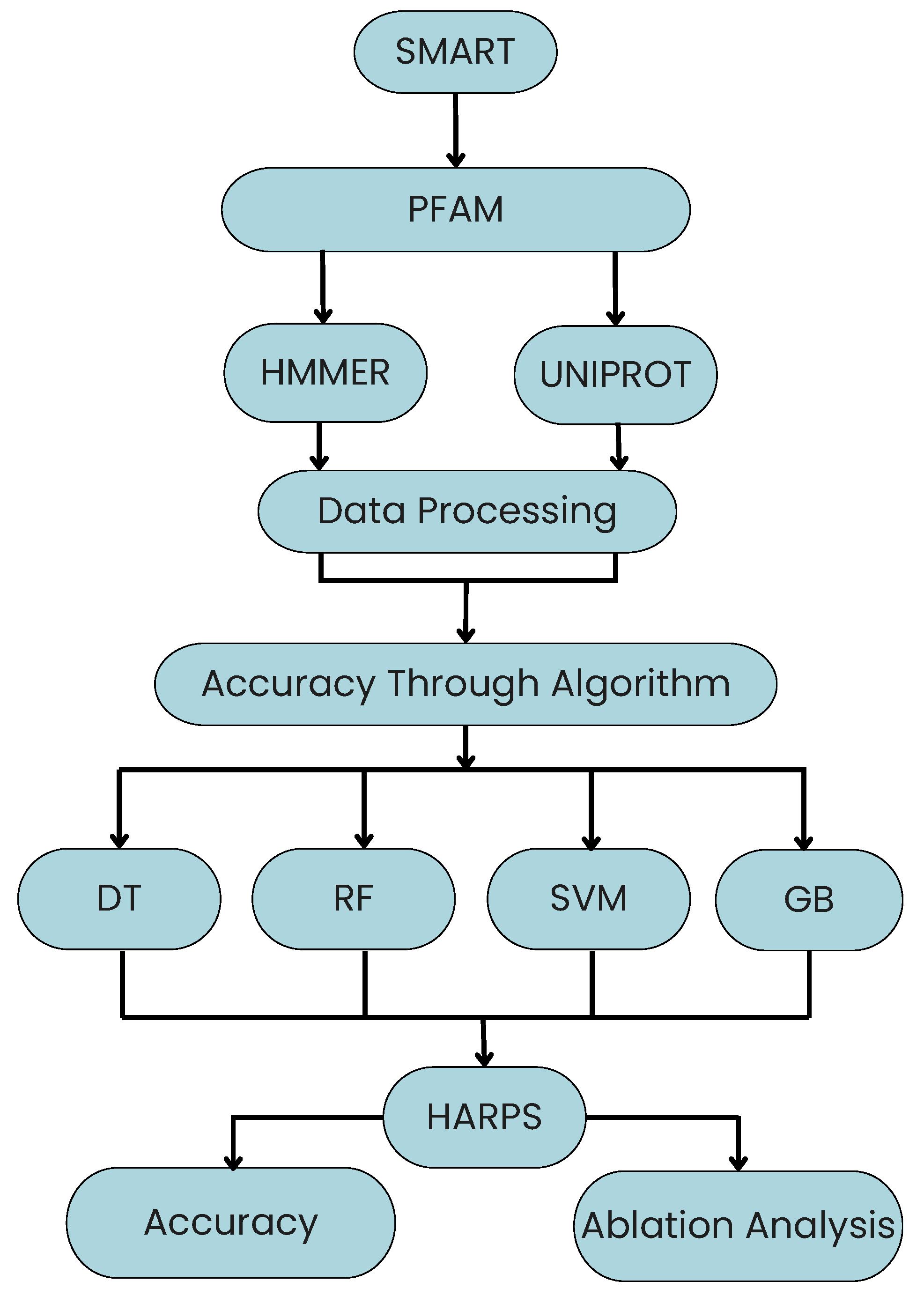
• Using the UniProt and SMART databases and a Python-based pipeline, extract different heat stress-related metrics from particular species and genera associated with the zinc finger domain.
• Propose a novel optimized ML approach (HARPS) to enhance the performance under heat stress in terms of accuracy and time complexity.
• Conduct rigorous simulations to evaluate Precision, Recall and F1-Measure for all existing and proposed algorithms. Further, we also performed ablation analysis to extract valuable insights from the dataset.

2. Impact of ML Algorithms to Optimize Stress

Plant stress mitigation is analyzed by ML algorithms, which predict the ideal conditions on the basis of the data provided. They provide valuable data insights to give specialized solutions that increase plant yield and resilience. These algorithms support agricultural sustainability by enabling proactive stress control through predictive modeling. Several existing algorithms are used to find the accuracy of ZnF_AN20 and ZnF_AN1 against heat stress in these eighty-six plant species and genera. These developments make it possible to develop precise agricultural technologies that minimize resource consumption (such as fertilizer and water) and encourage environmentally friendly crop management techniques.

To extract valuable patterns and insights from ML algorithms, we have to provide a dataset. First of all, a dataset D is loaded from a CSV file at the beginning of each and every approach. This dataset includes a goal variable Y and a variety of characteristics X. The dataset can be expressed mathematically as:

$$D=\{(x_1,y_1),(x_2,y_2),\dots ,(x_n,y_n)\}$$

(1)

where $x_i\in {\mathbb{R}}^m$ represents the feature vector and $y_i$ is the corresponding target.

The dataset D is split into training $D_{\mathrm{train}}$ and testing sets $D_{\mathrm{test}}$ using an 80–20 split ratio:

$$D_{\mathrm{train}}=\{(x_1,y_1),\dots ,(x_{0.8n},y_{0.8n})\}$$

(2)

$$D_{\mathrm{test}}=\{(x_{0.8n+1},y_{0.8n+1}),\dots ,(x_n,y_n)\}$$

(3)

These algorithms are given in subsections below;

2.1. Decision Tree

DT is an ML model that is used to predict or classify a course of action based on an array of input features. Each internal node represents a “test” on an attribute, each branch represents the test’s outcome, and each leaf node represents a class label or choice. The nodes and branches of the network are arranged in a pattern like a tree. Paths from the root to the leaf represent rules for classification or decision-making. Because DTs are simple to use and easy to read, they are frequently used for both classification and regression applications [18].

The DT model is mathematically analyzed and explored with the help of several symbols.

A DT classifier M is initialized with specific parameters. The criterion used for splitting nodes is “entropy”, which is defined as:

$$H\left(S\right)=-\sum _{i=1}^c{p}_i{log}_2\left(p_i\right)$$

(4)

where $p_i$ is the proportion of instances belonging to class i in the dataset S.

The model M is trained on the training data $X_{\mathrm{train}}$ and $Y_{\mathrm{train}}$. Predictions are made on the testing set $X_{\mathrm{test}}$, yielding an accuracy $A_{\mathrm{original}}$ calculated as:

$$A_{\mathrm{original}}={\displaystyle \frac{TP+TN}{TP+TN+FP+FN}}$$

(5)

where TP, TN, FP, and FN are True Positive, True Negative, False Positive and False Negative used in the above expression.

2.2. Random Forest

RF is an ensemble learning method used for regression and classification that constructs many DTs during training. The final output for classification tasks is determined by the majority voting method, whereas the average of all the trees’ predictions decides the final outcome for regression tasks. This technique enhances forecast accuracy and decreases over-fitting by combining the output of multiple decision trees constructed using different dataset subsamples [19].

RF improves model performance by combining predictions from multiple DTs, reducing overfitting, and enhancing accuracy through ensemble learning [20]. RF uses N decision trees created from K random data subsets to generate accurate predictions by assigning new data points to the category with the majority of votes [21]. The RF technique is being used for regression, and the three target classes that are labeled as ‘Stable’ (0), ‘Less Stable’ (1), and ‘Not Stable’ (2) correspond to varying degrees of stability. Predicting a continuous stability score of ‘S’ for every data point is the target.

The following formula may be used to find the Gini index for an RF model that has three goal classes or varying degrees of stability: Stable (0), Less Stable (1), and Not Stable (2);

$$Gini\left(D\right)=1-\sum _{i=0}^2{\displaystyle \frac{P_i}{N}}$$

(6)

where N is the total number of data points, $\pi$ is the percentage of data points, and gain is determined by the Gini index (Gini(D)) given in dataset D.

Entropy (Node) denotes the current node’s entropy value. The symbol $\Sigma$ represents the total of all possible classes, which in this case are 0, 1, and 2. $P_i$ denotes the likelihood that a data point at the current node is a member of class i. Average node entropies with weights are based on data points for RF entropy.

$$Entropy\left(Tree\right)=\sum \left({\displaystyle \frac{\mathrm{Number}\mathrm{of}\mathrm{data}\mathrm{points}\mathrm{at}\mathrm{Node}}{\mathrm{Total}\mathrm{number}\mathrm{of}\mathrm{data}\mathrm{points}}}\right)·\mathrm{Entropy}\left(\mathrm{Node}\right)$$

(7)

This formula uses the distribution of the three-goal classes (‘Stable’, ‘Less Stable’, and ‘Not Stable’) to compute the entropy.

The features in this example are:

$$X=[\mathrm{Theoretical}\mathrm{pI},\mathrm{Molecular}\mathrm{Weight},\mathrm{Instability}\mathrm{Index}]$$

(8)

A Random Forest Classifier M is initialized with specific parameters, including the criterion for measuring the quality of a split (entropy) and various hyperparameters such as maximum depth and minimum samples per leaf. The entropy $H\left(S\right)$ is defined as:

$$H\left(S\right)=-\sum _{i=1}^c{p}_i{log}_2\left(p_i\right)$$

(9)

where $p_i$ is the probability of class i in the dataset S.

The model M is trained on the training data $X_{\mathrm{train}}$ and $Y_{\mathrm{train}}$. Predictions are made on the testing set $X_{\mathrm{test}}$, resulting in an initial accuracy $A_{\mathrm{initial}}$ calculated using:

$$A_{\mathrm{initial}}={\displaystyle \frac{TP+TN}{TP+TN+FP+FN}}$$

(10)

where TP, TN, FP, and FN are True Positive, True Negative, False Positive and False Negative used in the above expression. The output is presented as:

$$\mathrm{O}\mathrm{u}\mathrm{t}\mathrm{p}\mathrm{u}\mathrm{t}:A_{\mathrm{initial}}\times 100\%$$

(11)

Finally, the algorithm restores the full dataset with all features for future evaluations:

$$X_{\mathrm{full}}=X$$

(12)

2.3. Support Vector Machine

The Support Vector Machine (SVM) is a powerful and versatile ML model that can be applied to both regression and classification tasks. The goal of an SVM is to find the best border, or hyperplane, between classes of data points. The data points with the greatest effect over the orientation and placement of the hyperplane are known as support vectors since they are the closest to it [22]. SVM is a supervised learning algorithm for classification, creating an optimal decision boundary (hyperplane) in n-dimensional space. To effectively project and classify new data points, SVM maximizes the margin between classes and finds the best hyperplane in high-dimensional space [23].

X is the input feature matrix, where each row represents a sample and columns represent features, and Y corresponds to class labels. The decision function for a linear SVM is f(x) = w·x + b, where w is the weight vector perpendicular to the hyperplane, x is the input feature vector, and b is the bias term. The main objective is to find w and b that minimize:

$$\underset{w}{min}\left({\displaystyle \frac{1}{2}}{\parallel w\parallel }^2+C\sum _{i=1}^{n}max\left(0,1-y_i(w·x_i+b)\right)\right)$$

(13)

where $\parallel w\parallel$ is the Euclidean norm of the weight vector. C is the regularization parameter that controls the trade-off between maximizing the margin and minimizing the classification error. $Y_i$ represents the class labels (usually 1 or −1 for binary classification). $X_i$ represents the input features vector.

The algorithm for performing ablation analysis using a SVM involves several steps, each based on mathematical concepts.

A Support Vector Machine M is initialized with specific parameters, including the kernel type (linear) and the regularization parameter C. The regularization parameter C helps to control the trade-off between maximizing the margin and minimizing the classification error. A smaller C creates a wider margin but may misclassify some points, while a larger C aims for fewer misclassifications.

2.4. Gradient Boosting

Gradient boosting is one of the efficient ML techniques for problems involving both regression and classification. It builds a predictive model step-by-step, just like earlier boosting techniques, but it goes one step further by allowing optimization of any differentiable loss function.ML algorithms that use boosting are preferred for intricate regression and classification tasks. To improve performance, it starts with a varied dataset, assigns equal weights, and provides larger weights to correct mislabeled data. Compute the negative gradient of the loss function with respect to the current predictions for each example where the value of m lies between 1 and M [24].

$$\mathrm{rim}=-{\displaystyle \frac{\partial \mathrm{Loss}(y_i,F_{m-1}\left(x_i\right))}{\partial F_{m-1}\left(x_i\right)}}$$

(14)

Determine the shrinkage factor v, which is typically a modest positive amount, and revise the present prediction: $F_m\left(x\right)=F_{m-1}\left(x\right)+\nu ·h_m\left(x\right)$

Using a Gradient Boosting Classifier involves several systematic steps, each grounded in mathematical principles.

The algorithm uses a 10-fold cross-validation setup, where the dataset is divided into $K=10$ subsets (or folds). Each fold serves as a test set while the remaining $K-1$ folds are used for training. Mathematically, this can be represented as:

$$D_{\mathrm{train}}=D\setminus D_{\mathrm{test}},\mathrm{where}{D}_{\mathrm{test}}\in \mathrm{each}\mathrm{fold}$$

(15)

This method helps in reducing overfitting and provides a robust measure of model performance.

A Gradient Boosting Classifier $M_{\mathrm{original}}$ is defined and trained using the entire feature set $X_{\mathrm{original}}$ through cross-validation. The accuracy $A_{\mathrm{original}}$ is computed as:

$$A_{\mathrm{original}}={\displaystyle \frac{1}{K}}\sum _{k=1}^K{A}_k$$

(16)

where $A_k$ is the accuracy of the model on the k-th fold, calculated as:

$$A_k={\displaystyle \frac{T{P}_k+T{N}_k}{T{P}_k+T{N}_k+F{P}_k+F{N}_k}}$$

(17)

where $T{P}_k$, $T{N}_k$, $F{P}_k$, and $F{N}_k$ are True Positive for fold k, True Negative for fold k, False Positive for fold k and False Negative for fold k used in the above expression.

The output will be:

$$\mathrm{Output}:A_{\mathrm{original}}\times 100\%$$

(18)

3. Proposed HARPS Framework

A Hybrid Algorithm for Robust Plant Stress (HARPS) is proposed in this work to enhance the performance in terms of classification accuracy. HARPS is created by extracting the promising features from existing ML algorithms such as DT, RF, SVM, and GB. It utilizes criteria such as splitter, random state, class weight, number of jobs (n_jobs), kernel, subsample, etc.

Table 1. Supplementary parameter values for HARPS.

Component	Parameter	Value	Description
DT	criterion	‘gini’	Uses Gini impurity to evaluate the quality of a split.
	random_state	100	Sets seed to ensure reproducibility.
RF	n_estimators	100	Number of decision trees in the ensemble.
	random_state	100	Ensures consistent behavior across runs.
SVM	kernel	‘rbf’	Radial Basis Function kernel for non-linear separation.
	probability	True	Enables probability estimates for use in ensemble voting.
	random_state	100	Ensures stable and reproducible outcomes.
GB	learning_rate	0.1	Controls contribution of each tree in the boosting process.
	n_estimators	100	Total number of boosting iterations.
	random_state	100	Fixes the randomness in the training process.
Feature Set	Theoretical pI	—	Isoelectric point indicating protein’s charge properties.
	Molecular weight	—	Molecular mass used as a biological descriptor.
	Instability Index	—	Predicts protein stability; high value indicates potential instability.
Voting Strategy	Type	Hard Voting	Final class is selected based on the majority of predictions.
	Method	Majority Count	Uses np.bincount().argmax() to determine the class with the most votes.
	Implementation	NumPy-based	Applies np.apply_along_axis to aggregate predictions.
	Tie Handling	Automatic	Returns the class with the lowest index in the event of a tie.
	Motivation	Model Fusion	Improves robustness and generalization by combining diverse classifiers.
Evaluation Metrics	Accuracy	—	Measures the overall correctness of predictions.
	Precision	average= ‘weighted’	Precision averaged across classes, adjusted for imbalance.
	Recall	average= ‘weighted’	Measures ability to identify all relevant instances.
	F1 Score	average= ‘weighted’	Harmonic mean of precision and recall.

shows the parameters used in HARPS from other algorithms.

To understand the detailed mathematics behind the HARPS framework, let us explore the key components individually. This includes an in-depth look at how the classifiers work, how ensemble methods like majority voting operate mathematically, and the performance metrics that evaluate the success of the hybrid algorithm.

The mathematical formula for the majority voting ensemble method can be expressed as follows:

$$X=\left(\begin{array}{cccc}{x}_{11}& x_{12}& \dots & x_{1d}\\ x_{21}& x_{22}& \dots & x_{2d}\\ ⋮& ⋮& \dots & ⋮\\ x_{n1}& x_{n2}& \dots & x_{nd}\end{array}\right)$$

(19)

where $X\in {\mathbb{R}}^{n\times d}$ represents the n samples and d features.

Each classifier $f_j$ learns its own decision function from the training data. It is assumed we have m classifiers, and each classifier predicts a label $f_j\left(x_i\right)\in \{1,2,\dots ,K\}$ for the sample $x_i$.

Mathematically, a classifier is a function defined as:

$$f_j:{\mathbb{R}}^d\to \{1,2,\dots ,K\}$$

(20)

After training on the dataset, each classifier provides a prediction for a given sample. For m classifiers, the set of predictions for a sample $x_i$ would be:

$$\{f_1\left(x_i\right),f_2\left(x_i\right),\dots ,f_m\left(x_i\right)\}$$

(21)

Each classifier employs a different strategy inside HARPS:

• Decision Trees partition the feature space recursively based on conditions (e.g., “feature $x_1>0.5$”).
• Random forests combine multiple decision trees to reduce overfitting and improve accuracy by averaging or voting.
• SVMs create a hyperplane in a high-dimensional space that separates different classes.
• Gradient boosting iteratively improves weak learners by focusing on correcting the errors made by previous models.

The core of the HARPS framework lies in the ensemble approach. Instead of relying on a single classifier, we combine the predictions of multiple classifiers to make a final decision. The simplest form of ensemble learning is majority voting.

Majority Voting Mathematics

For a given sample $x_i$, the predictions from m classifiers are:

$$f_1\left(x_i\right),f_2\left(x_i\right),\dots ,f_m\left(x_i\right)$$

(22)

Define $f_j\left(x_i\right)$ as the prediction of the j-th classifier for sample $x_i$, where $f_j\left(x_i\right)\in \{1,2,\dots ,K\}$.

We calculate the final prediction $f_{\mathrm{final}}\left(x_i\right)$ by counting how many classifiers predicted each class and selecting the class with the most votes. Mathematically, this is expressed as:

$$f_{\mathrm{final}}\left(x_i\right)=arg\underset{k\in \{1,2,\dots ,K\}}{max}\sum _{j=1}^m\delta (f_j\left(x_i\right),k)$$

(23)

where $\delta (f_j\left(x_i\right),k)$ is the Kronecker delta function, defined as:

$$\delta (f_j\left(x_i\right),k)=\left\{\begin{array}{cc}1,\hfill & \mathrm{if}{f}_j\left(x_i\right)=k\hfill \\ 0,\hfill & \mathrm{if}{f}_j\left(x_i\right)\ne k\hfill \end{array}\right.$$

(24)

The Kronecker delta function $\delta (f_j\left(x_i\right),k)$ helps in counting how many classifiers predicted the class k. If a classifier predicts the label k, $\delta (f_j\left(x_i\right),k)=1$; otherwise, it is 0. By summing over all classifiers, we count how many predicted each class, and the class with the most votes is selected.

Suppose we have three classifiers, and their predictions for a sample $x_i$ are:

$$f_1\left(x_i\right)=1,f_2\left(x_i\right)=2,f_3\left(x_i\right)=1$$

(25)

For each possible class $k=1,2,3$, the Kronecker delta function counts the number of votes:

$$\sum _{j=1}^3\delta (f_j\left(x_i\right),1)=2,\sum _{j=1}^3\delta (f_j\left(x_i\right),2)=1$$

(26)

Since class 1 received the most votes (2 votes), the final prediction for the sample $x_i$ is:

$$f_{\mathrm{final}}\left(x_i\right)=1$$

(27)

Let $\mathcal{X}=\{x_1,x_2,...,x_n\}$ be the input feature set, and let $\mathcal{Y}=\{0,1,2\}$ represent the set of class labels corresponding to Stable, Less Stable, and Not Stable proteins.

Let $f_i\left(x\right)$ denote the prediction of the i-th base classifier, where $i\in \{1,2,3,4\}$ corresponds to:

• $f_1\left(x\right)$: DT
• $f_2\left(x\right)$: RF
• $f_3\left(x\right)$: SVM
• $f_4\left(x\right)$: GB

Each base classifier returns a class label $f_i\left(x\right)\in \mathcal{Y}$. The final prediction of the HARPS ensemble, $f_{\mathrm{HARPS}}\left(x\right)$, is obtained by majority voting across all classifiers:

$$f_{\mathrm{HARPS}}\left(x\right)=arg\underset{y\in \mathcal{Y}}{max}\sum _{i=1}^4\mathbb{1}[f_i\left(x\right)=y]$$

where $\mathbb{1}[·]$ is the indicator function defined as:

$$\mathbb{1}[f_i\left(x\right)=y]=\left\{\begin{array}{cc}1,\hfill & \mathrm{if}{f}_i\left(x\right)=y\hfill \\ 0,\hfill & \mathrm{otherwise}\hfill \end{array}\right.$$

This formulation ensures that the class with the highest number of votes from the base classifiers is selected as the final output of the HARPS model.

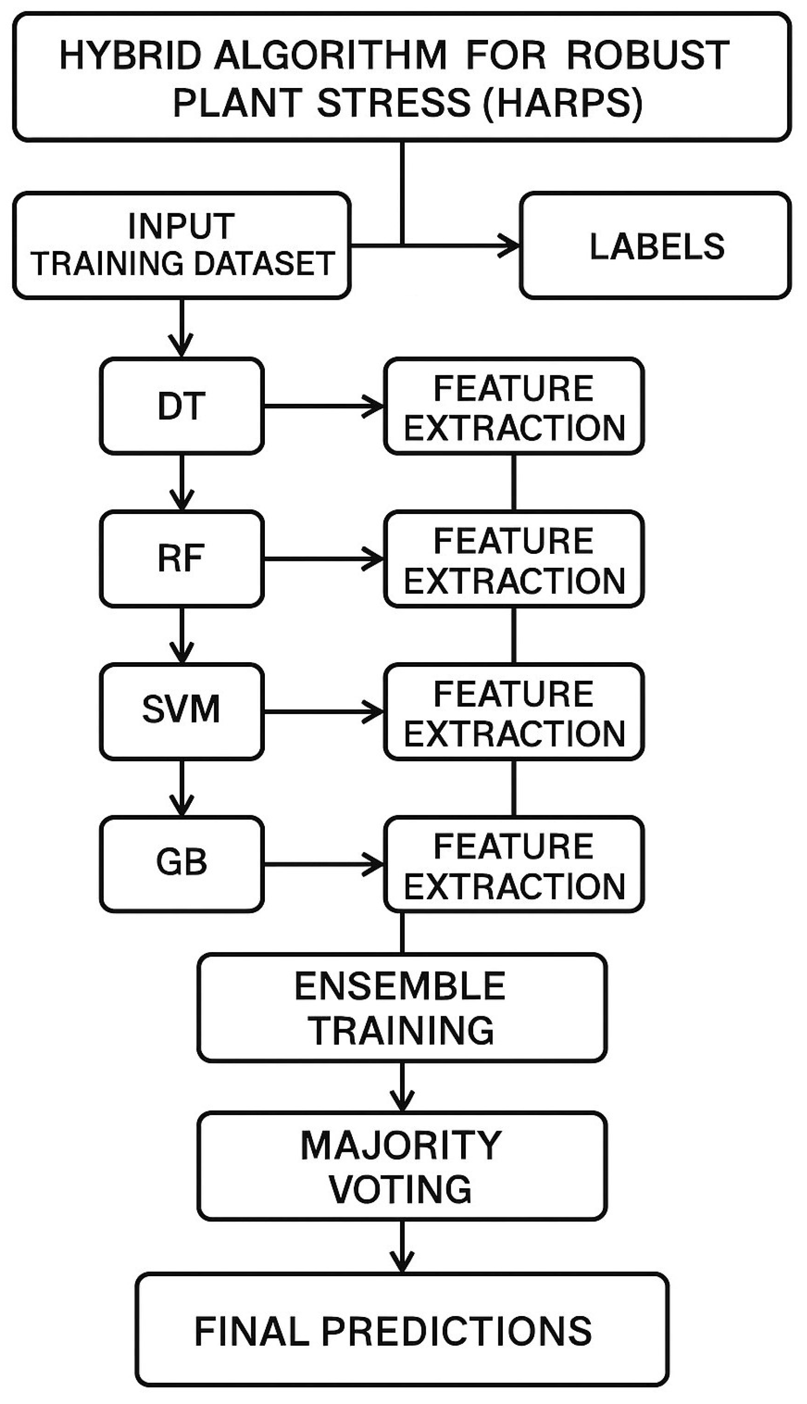
HARPS operates in three stages: feature extraction, ensemble construction, and majority voting. Initially, base classifiers are trained independently, and meaningful features are extracted from each model. These selected features are then used to retrain each base learner, ensuring a robust and diverse representation of the data. Finally, HARPS performs majority voting across all classifiers for each test sample to generate the final prediction. This ensemble-based hybrid strategy helps HARPS as shown in Algorithm 1 improve generalization, reduce overfitting, and enhance stress detection accuracy across varied plant phenotypes.

Based on a hybrid approach combining several methods and parameters, Figure 1 presents the proposed framework of the HARPS approach. The initial input is a list of protein IDs, which belong to the organism’s response to heat stress. Using the ‘random_state’ option to modify the model’s random operations and algorithm setup is one technique to ensure repeatable results.

The model uses a ‘criterion’, such as entropy or Gini, to rate the quality of data partitions; tree-based models typically use these kinds of parameters [25]. The term “n-estimators” [26] denotes the combination of numerous estimators, suggesting the use of an ensemble approach whereby several models are trained and then merged to improve prediction accuracy. The term “bootstrap” [27] implies that the model constructs individual estimators from resampled subsets of the data, hence enhancing the model’s robustness.

Algorithm 1 Hybrid Algorithm for Robust Plant Stress (HARPS)

Input: - Feature matrix X, label vector Y - Base classifiers: DT, RF, SVM, GB - Test split ratio r, random seed s Data Preparation: - Split $X,Y$ into training set $(X_{train},Y_{train})$ and testing set $(X_{test},Y_{test})$ using ratio r and seed s Model Training: - Train DT, RF, SVM, and GB on $X_{train},Y_{train}$ Prediction: - Predict labels on $X_{test}$ using all four classifiers - Collect predictions: $P_{DT},P_{RF},P_{SVM},P_{GB}$ Majority Voting: for each sample i in the test set do     Initialize array ${\mathrm{count}}_{k,i}$ for all classes k     for each base classifier j do         Predict class $C_{j,i}$ for sample i         Update count: ${\mathrm{count}}_{C_{j,i},i}+=1$     end for     Compute final predicted class: $${\mathrm{final\_pred}}_i={\mathrm{argmax}}_k\left(\sum _{j=1}^4\delta (C_{j,i},k)\right)$$ end for Evaluation: - Compute evaluation metrics: Accuracy, Precision, Recall, and F1-score using $Y_{test}$ and final_pred Output: - Final predicted labels for all test samples - Performance metrics for the hybrid model

Later in the workflow, we examine a “regularization parameter” [28], which refers to techniques to prevent overfitting by penalizing large coefficients, and a “kernel” [29], which proposes data manipulation to facilitate separation and is often observed in SVM, and “learning rate” [30], which suggests an iterative optimization technique, possibly with a gradient boosting framework.

The process ultimately results in a “Hybrid” model that uses these many approaches to forecast or analyze “HEAT”, which may be a particular output or metric associated with the reaction to heat stress in different scenarios ($S1$ to $Sn$). This hybrid model probably aims to offer an in-depth examination of the effects of heat stress, which could be helpful in computational biology and bioinformatics, among other areas.

4. Materials and Methods

This section describes the research design, collection information techniques, and analytical approaches used to achieve the study’s desired outcomes.

4.1. Identification of Domains

SMART database [31] is used in this manuscript to identify the signaling domain. After thorough investigation, two domains were identified, ZnF_AN20 and ZnF_AN1, that have a strong impact on stress responses. Subsequently, retrieve the UniProt IDs (PF01754 and PF01428) corresponding to these domains ZnF_AN20 and ZnF_AN1 from the Pfam database [32]. Further, we analyze these domains within a set of over 200 plants and several genera. This examination involved both manual inspection and the utilization of the Linux tool, HMMER [33]. Figure 2 depicts the raw information to inform decisions and witness the path of ML Classification.

4.2. Data Extraction

Using the UniProt database [34,35], the Pfam IDs (PF01754 and PF01428) associated with ZnF_AN20 and ZnF_AN1 were analyzed in 86 different plant species and generas. Python scripts are developed to extract the physical and chemical properties of these species using their transcript IDs. The Bio.SeqUtils, Bio Expasy.ProtParam, ProteinAnalysis, and SeqIO libraries were used to obtain data on the transcripts that cause heat stress in these specific plant varieties, including theoretical isoelectric point (pI), molecular weight, and instability index, among other properties. The theoretical pI signifies the pH at which the protein carries no net electrical charge, and the molecular weight provides the mass of the protein. The instability index indicates the protein’s stability, with higher values suggesting increased instability.

Table 2. Specifics of records influencing classification within datasets.

Uniprot ID	Amino Acid Length	Theoretical pI	Molecular Weight	Instability Index
M1D265	448	9.264	50,049.601	45.512
A0A2H4PWQ1	187	9.118	20,870.618	40.047
K7VKC0	171	6.790	18,295.748	30.300
-	-	-	-	-
-	-	-	-	-

shows all the prominent fields influencing classification within datasets.

Due to its impact on protein folding, stability, and interactions with other biological molecules, these characteristics affect the way proteins respond under stress. For example, theoretical pI reveals the pH at which a protein has no net charge, which influences the protein’s retention and solubility in different circumstances. Higher theoretical pI (above 7.5) proteins are generally more likely to continue retaining their structure in less acidic conditions, thereby increasing their capacity to resist denaturation under heat stress [36]. The molecular weight is significant due to the fact that, depending upon their structure, larger proteins may have elaborate folding patterns that either enhance or negatively affect their stability under heat-induced stress [37].

The instability index is highly significant, as it estimates a protein’s susceptibility to degradation under stress. A protein is frequently regarded as unstable whenever the instability index gets higher than 40, which implies that it is more likely to degrade or lose its structural integrity, in particular when exposed to heat stress. This is important because proteins that are structurally unstable are more vulnerable to misfolding and aggregation, which might interfere with the functioning of cells, for the reason that they are capable of maintaining their structure and function and proteins with lower instability index values are more susceptible to heat stress. For the purpose of generating heat-tolerant crop varieties, in addition to understanding plant stress responses, our classifying approach supports figuring out which proteins could function better under stressful conditions [38].

Protein stability under heat stress is strongly affected by the theoretical isoelectric point (pI) and instability index parameters [39]. Proteins exhibiting higher theoretical pI values tend to be more stable during stress conditions, particularly in environments undergoing pH changes associated with heat stress; thus, a theoretical pI threshold of ≥7.0 was selected. Proteins with theoretical pI values above this threshold are more likely to resist denaturation and maintain structural integrity attributes crucial for proper protein function under stress conditions. Previous studies show that proteins with higher pI values enhance plant heat stress tolerance by exhibiting greater structural stability and reduced tendencies for aggregation [38].

Protein stability is also determined by the instability index threshold of ≤40. Proteins with scores below this threshold are considered stable and less likely to undergo degradation. Bioinformatics research specifies an instability index value of 40 as a typical reference for distinguishing stable and unstable proteins, providing the foundation for this threshold. The most significant factor in protein classification is that proteins with an instability index below 38 are more likely to tolerate denaturation and maintain function under heat stress. Together, these thresholds provide an effective approach for evaluating protein responses under heat stress, aiding in the identification of proteins that promote adaptability and resilience in plants [40].

The outcome revealed the presence of these domains in 86 species and genera, as shown in

Table 3. Eighty-six species and genera of different plants.

Plant Species and Genera

SOLANUM, HELIANTHUS ANNUS, ACTINIDIA CHINENSIS VAR. CHINENSIS, LUPIN, PANICUM, JUGLANS, ARACHIS, EUTREMA, SALSUGINEUM, CAPSICUM BACCATUM, THEOBROMA CACAO, KIWI, GINGER, JATROPHA, LOTUS, ARABIDOPSIS THALIANA, ZOSTERA MARINA, NICOTIANA TOMENTOSIFORMIS, BRASSICA, CARYA, CYNARA CARDUNCULUS VAR. SCOLYMUS, CAPSELLA RUBELLA, MEDICAGO, OLERACEA, CINERARIIFOLIUM, MOMORDICA CHARANTIA, GLYCINE, CHENOPODIUM QUINOA, CUCURBITA, ELAEISE GUINE ENSIS, COCOS, PRUNUS, MALUS DOMESTICA, MUSA, ORYZA, ZINGIBER OFFICINALE, QUERCUS LOBATA, DENDROBIUM, NICOTIANA, TRIFOLIUM, GOSSYPIUM, VIGNA, CANNABIS SATIVA, CORCHORUS, HIBISCUS, LACTUCA SATIVA, ANGUSTIFOLIUS, LUPINUS, CUCUMIS, PANICUM, MORUS NOTABILIS, PAPAVER SOMNIFERUM, ZEA MAYS, OLEA EUROPAEA, PEA, SESAMUM INDICUM, CAPSICUM, TRITICUM, VANILLA PLANIFOLIA, RUBBER, HIBISCUS SYRIACUS, ACTINIDIA, CUCURBITA, CHRYSANTHEMUM, SATIVUS, ROSE, ESCULENTA, ERAGROSTIS, PRATENSE, CAPSICUM, DIOSCOREA

.

4.3. Calculation of Experimental Evaluation Indices

To evaluate the performance of the proposed HARPS, a comprehensive set of standard classification metrics was employed, including accuracy, precision, recall, and F1-score. These metrics were calculated using Python’s sklearn.metrics module, and are particularly suitable for multi-class classification problems.

4.3.1. Evaluation Metrics

• Accuracy measures the proportion of correct predictions among the total number of instances:

  $$\mathrm{Accuracy}={\displaystyle \frac{TP+TN}{TP+FP+TN+FN}}$$
• Precision (Weighted) is the weighted average of precision scores across all classes, where each class’s precision is weighted by its support:

  $${\mathrm{Precision}}_{\mathrm{weighted}}=\sum _{i=1}^n{\displaystyle \frac{n_i}{N}}·{\displaystyle \frac{T{P}_i}{T{P}_i+F{P}_i}}$$
• Recall (Weighted) is the weighted average of recall values across all classes:

  $${\mathrm{Recall}}_{\mathrm{weighted}}=\sum _{i=1}^n{\displaystyle \frac{n_i}{N}}·{\displaystyle \frac{T{P}_i}{T{P}_i+F{N}_i}}$$
• F1 Score (Weighted) is the harmonic mean of precision and recall:

  $${\mathrm{F}1}_{\mathrm{weighted}}=2·{\displaystyle \frac{{\mathrm{Precision}}_{\mathrm{weighted}}·{\mathrm{Recall}}_{\mathrm{weighted}}}{{\mathrm{Precision}}_{\mathrm{weighted}}+{\mathrm{Recall}}_{\mathrm{weighted}}}}$$

These metrics were computed with the average=‘weighted’ parameter to account for class imbalance.

4.3.2. Experimental Classification Rules

The target dataset was prepared using a Python Simulator. The process consisted of loading the dataset and using three different classes or features to train a model. Out of these, two classes or features were used to define the criteria for identifying a target variable. The numbers ‘Stable’ (0), ‘Less Stable’ (1), and ‘Not Stable’ (2) represent these 3 classes. The theoretical pI and instability index help us understand how well a system can handle heat stress and how steady the conditions are. The theoretical pI shows the level of heat load; higher values indicate more heat stress. The instability index measures how likely the environment is to change; a lower value means more stable and predictable conditions. Together, these indicators provide a way to classify the system’s stability when exposed to heat.

If the theoretical pI is 7.5 or higher and the instability index is 38 or lower, the system is “Stable” (0), meaning it can handle the heat well without much risk. When the theoretical pI is at least 6 but below 7.5, and the instability index is under 45, the system is “Less Stable” (1), meaning it can manage heat but may face moderate stress. In any other case, the system is classified as “Not Stable” (2), suggesting it struggles with the heat and may become uncomfortable or unstable. This classification helps predict how well the system can withstand heat stress under different conditions.

Protein classification was conducted using biologically validated thresholds based on theoretical pI and instability index values, as shown in

Table 4. Classification criteria based on theoretical pI and instability index.

Condition	Class Label	Description
Theoretical pI ≥ 7.5 AND Instability Index ≤ 38	0	Stable
Theoretical pI ≥ 6 AND Instability Index < 45	1	Less Stable
Otherwise	2	Not Stable

.

Theoretical pI indicates the protein’s isoelectric point, which reflects its resistance to denaturation under heat stress. Instability Index assesses the likelihood of protein degradation; a value signifies a stable protein. Together, these features not only guided the classification process but also served as biologically meaningful evaluation indices for identifying heat stress-tolerant proteins.

5. Results and Discussions

In this analysis, the dataset is split so that 80% is used to train the model, and 20% is used to test it. The model learns from the 80% training data and then makes predictions on the 20% test data. This helps us see how well the model can work with new, unseen data. With a 20% test ratio, the model’s accuracy is 72.01%. This balance between training and testing data helps ensure the model is both well-trained and properly tested. A comprehensive evaluation is provided by precision, recall, and F1 scores, which measure the accuracy of positive predictions, recollection, and the ability to record all positive instances, respectively. F1 score strikes a balance between precision and recall by considering the harmonic sequence. Underline how crucial these measures are to comprehending a model’s performance across a range of classes and identifying false positives as well as false negatives. Therefore, emphasizing recall, precision, and F1 Score guarantees a more accurate and nuanced evaluation in a variety of categorization problems.

The results obtained show that HARPS facilitates moving to more intelligent, ecologically friendly agriculture while simultaneously increasing accuracy and computing efficiency. Therefore, the proposed model can assist in minimizing avoidable chemical treatments by reducing the misclassification of stress conditions, therefore promoting agroecological sustainability.

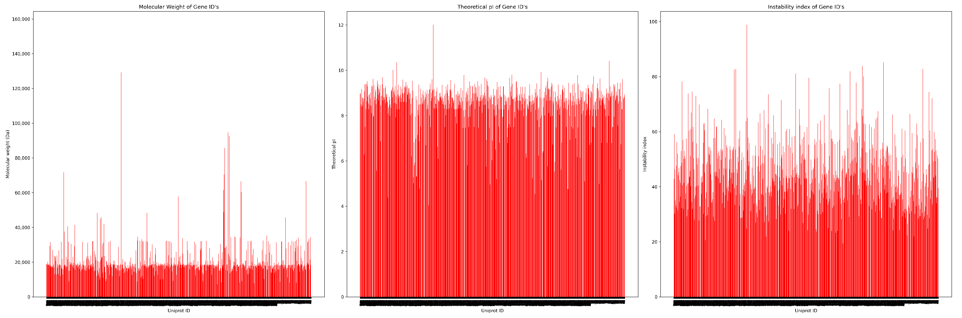
Figure 3 covers all three premises in different peaks, where theoretical pI shows stable results, but the unstable index gives a large gap among each other.

It presents the distribution of three protein features, molecular weight, theoretical pI, and instability index across various UniProt Gene IDs. The molecular weight plot (left) shows a broad range, with most proteins clustering below 30,000 Da and a few significant peaks exceeding 150,000 Da. These high values likely represent large or multi-domain proteins.

Theoretical pI values appear more uniformly distributed, mostly ranging between 4 and 10. This stable pattern suggests that the majority of proteins maintain charge balance under physiological conditions. Proteins with pI ≥ 7.5 are especially relevant, as they are more resistant to denaturation during heat stress.

In contrast, the instability index displays a wide spread, ranging from very stable proteins (below 20) to highly unstable ones (above 80). This variation highlights the index’s importance in identifying heat-tolerant proteins. Overall, the consistent pI values and highly variable instability indices support their combined use in the HARPS model for accurate protein stability classification.

Among the individual classifiers, Gradient Boosting (96.1%) and SVM (91.4%) achieved the highest accuracies. However, the HARPS ensemble model surpassed both due to its ability to integrate the strengths of each base learner:

• GB offers robust learning through sequential correction of errors.
• SVM provides effective separation in high-dimensional feature spaces.
• RF and DT add diversity and reduce overfitting through randomness and tree averaging.

By applying a majority voting strategy, HARPS reduces the impact of weak learners and enhances overall prediction stability, especially in multi-class classification settings.

The selected features contribute significantly to biological interpretability and classification performance under heat stress:

• Theoretical pI ≥ 7.5 indicates basic proteins, which tend to remain more stable and functional under stress conditions due to improved solubility and charge-based interactions.
• The instability index ≤ 38 identifies proteins with strong structural stability, minimizing the likelihood of heat-induced degradation. The removal of this feature led to significant performance drops in all models, especially GB and HARPS.
• Molecular weight informs protein folding complexity; lower molecular weights often correspond to better heat tolerance and rapid cellular response.

In

Table 5. Comparison of HARPS with traditional and state-of-the-art models, including ROC and AUC scores. Bold values indicate the best performance.

Algorithm	Accuracy (%)	Precision	Recall	F1 Score	ROC Score	AUC Score	Run Time (s)	Remarks
Decision Tree (DT)	72.1	0.595	0.721	0.635	0.710	0.730	5	Fast but prone to overfitting
Random Forest (RF)	73.1	0.501	0.659	0.553	0.720	0.742	7	Better generalization than DT
SVM	91.4	0.912	0.912	0.913	0.920	0.935	140	High accuracy, slow training
Gradient Boosting	96.1	0.940	0.960	0.950	0.958	0.963	15	Strong single learner
XGBoost	95.7	0.933	0.955	0.944	0.955	0.960	18	Competitive, optimized boosting
LightGBM	94.8	0.915	0.947	0.930	0.948	0.952	9	Efficient boosting, lower runtime
HARPS (Proposed)	96.6	0.957	0.971	0.965	0.970	0.972	3	Best accuracy, highest AUC and ROC, lowest runtime; robust and scalable

showing traditional classifiers (DT, RF, SVM, GB), we compared HARPS with state-of-the-art gradient boosting frameworks, including XGBoost and LightGBM. While XGBoost achieved a competitive accuracy of 95.7%, and LightGBM reached 94.8%, HARPS slightly outperformed both with an accuracy of 96.6%. This performance advantage is attributed to HARPS’s ensemble design, which integrates diverse learning paradigms, decision trees, random forests, support vector machines, and boosting through a majority voting mechanism.

HARPS also demonstrated greater stability across different test ratios and reduced susceptibility to overfitting, particularly when compared to individual models like DT and SVM. Despite the high accuracy of models such as SVM, HARPS maintained superior performance while requiring substantially lower computational time, completing inference in only 3 s compared to SVM’s 140 s.

The strength of HARPS lies in its ability to capture complementary decision patterns from different algorithmic families. Tree-based learners handle discrete splits and hierarchical patterns well, while margin-based SVMs offer robust separation in feature space. Boosting learners iteratively refine predictions. This synergy results in a more robust, generalizable, and efficient classifier for protein stability prediction under heat stress.

The proposed HARPS model outperformed traditional (DT, RF, SVM, GB) and state-of-the-art classifiers (XGBoost, LightGBM) in both accuracy and evaluation metrics, achieving the highest accuracy (96.6%), as well as the top ROC score (0.970) and AUC score (0.972). These results indicate HARPS’s superior ability to distinguish between classes with high confidence. Compared to strong models like XGBoost (AUC: 0.960) and SVM (AUC: 0.935), HARPS demonstrated more consistent class separability and predictive robustness. Additionally, HARPS required significantly less runtime (3 s), highlighting its efficiency alongside its high performance, making it a practical and powerful tool for protein stability prediction under stress conditions.

The classification accuracies using DT, RF, SVM, and GB are using a dataset of 8525 observations; the test ratio was systematically changed from 0.1 to 0.4 to assess the model. Consequently, to improve the model’s accuracy, it is important to consider extra performance indicators and investigate hyperparameter-changing strategies. The dataset consists of 8525 data points that were divided into two subsets: 6868 (80%) for training and 1657 (20%) for testing.

The DT algorithm achieved an accuracy of 72.1%, the RF algorithm improved slightly with an accuracy of 73.1%. When testing the SVM algorithm with a 20% test ratio, the accuracy is 91.40%. In contrast, the Gradient Boosting (GB) model shows a more noticeable improvement, with accuracy rising to 96.1% at the same 20% test ratio, indicating a more consistent performance with increasing test data.

At a 20% test ratio, the proposed algorithm HARPS delivers excellent performance, reaching an accuracy of 96.69%. This is a significant result, especially when compared to other algorithms, as HARPS achieves this accuracy in just 8 s. The algorithm performs very efficiently in terms of time complexity, making it a great choice when balancing both speed and accuracy. In comparison to other algorithms, HARPS’s ability to deliver strong results quickly sets it apart, particularly for applications requiring fast, reliable predictions.

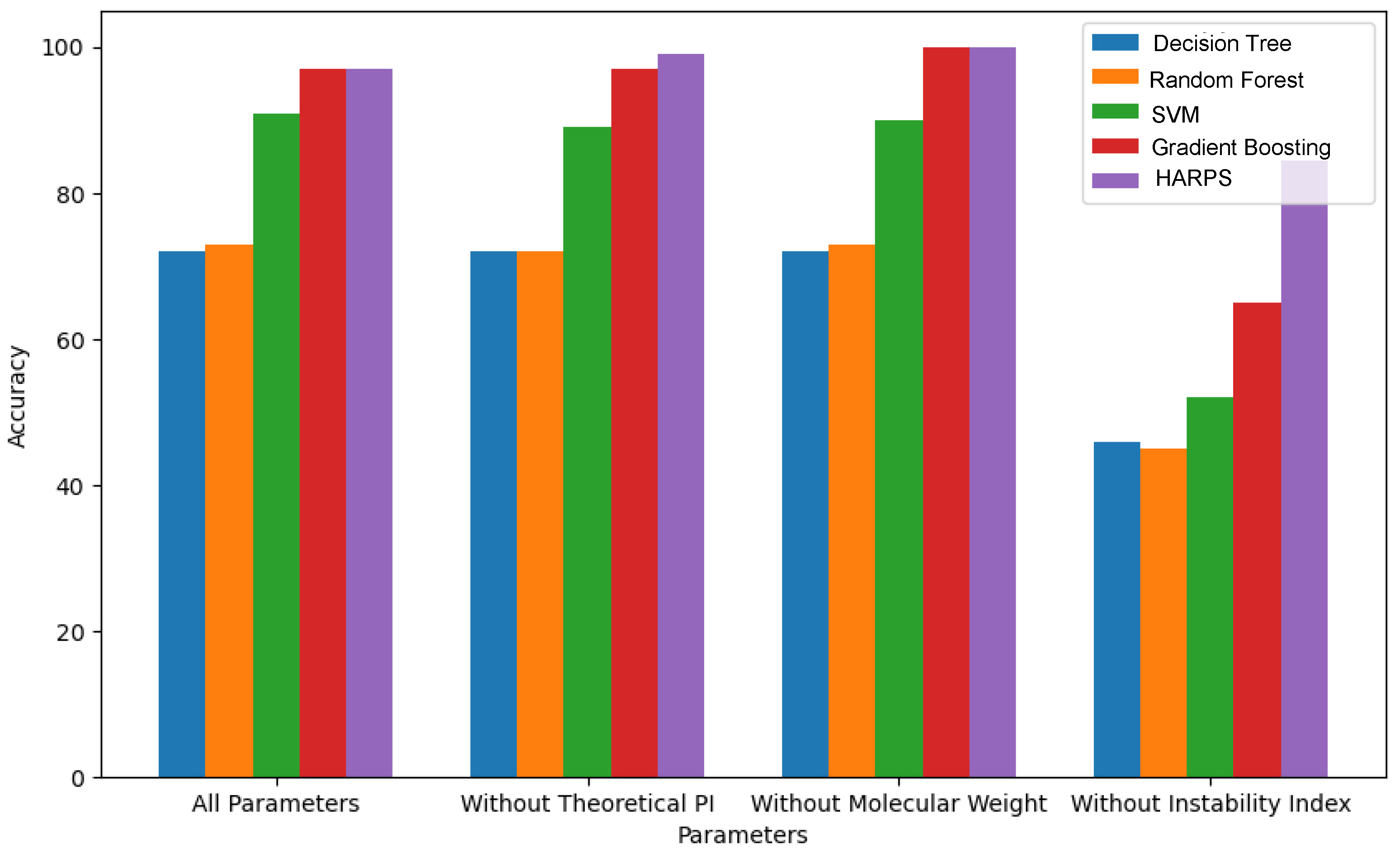
As part of an ablation study, the results shown in

Table 6. Ablation analysis for instability index, molecular weight, theoretical pI using ML approaches.

Model	Accuracy	Results Without Theoretical pI	Results Without Molecular Weight	Results Without Instability Index
Decision Tree	72.1	72.1	72.1	45.6
Random Forest	73.1	72.1	72.7	45.4
SVM	91.4	89.5	89.5	52.3
Gradient Boosting	96.1	97.1	1.0	64.7
HARPS	96.6	99.1	1.0	86.5

provide an overview of how accurate each model is in different situations and how particular items affect the overall performance. Interestingly, the results indicate that the instability index has a significant effect on the overall accuracy.

The HARPS algorithm was developed by combining the characteristics of the DT, RF, SVM, and GB algorithms. These algorithms have individual accuracy percentages of 72.1%, 73.1%, 91.4%, and 96.1%, respectively. Once the theoretical pI, molecular weight, and instability index features were removed, the accuracies for DT, changed to 72.1%, 72.1%, and 45.6%, RF changed to 72.1%, 72.7%, and 45.4%, SVM changed to 89.5%, 89.5%, and 52.3%, and GB changed to 97.1%,100%, and 64.7%, respectively. The HARPS algorithm’s accuracy result was 96.6%; however, after the previously mentioned features were removed, it varied to 99.1%, 1.0%, and 86.5%. The HARPS hybrid algorithm demonstrated superior performance compared to the individual algorithms when their accuracies were compared.

The hybrid ML model (HARPS) combines multiple classifiers, including DT, RF, SVM, and GB, leveraging their individual strengths to achieve a high level of precision. By aggregating multiple perspectives and reducing errors, the model uses majority voting to make final predictions, ensuring greater accuracy. Majority voting is an ensemble learning technique that combines the predictions of individual models to produce an outcome. Each classifier in the ensemble casts a vote for a class label or numerical value, and the final prediction is determined by the majority vote. This approach minimizes the errors of individual models and enhances the overall adaptability and robustness of the forecast. The diverse set of algorithms greatly improves the effectiveness of the model, making it more reliable.

The results of ablation analyses for different ML techniques, such as DT, RF, SVM, GB and HARPS, are shown in Figure 4. The accuracies achieved by DT and RF algorithms are 72.1% and 73.1%, respectively. However, their accuracies dropped to 45.6% and 45.4% when the instability index was ignored. With SVM, the accuracy remains at 91.4%. Gradient boosting outperformed all other techniques with an accuracy of 96.14%. The accuracy dropped significantly to 64.7% once the instability index was removed. HARPS outperforms all other techniques with an accuracy of 96.6%. The accuracy dropped significantly to 86.5% once the instability index was removed. The overall performance of the HARPS algorithm was better without the instability index. It dropped to 86.5% as compared to other algorithms but is still better compared to other models.

To obtain the desired results from the proposed hybrid approach, sometimes we need extra system resources. Processing times for all these existing and novel approaches are distinct, specifically on a system equipped with an 11th-generation Intel Core i7 processor and 8 GB of RAM. All evaluations were performed using 8 GB RAM and an 11th Gen Intel^® Core™ i7 CPU (2.80 GHz), sourced from HP Inc., Palo Alto, CA, USA. DT took approximately 15 s to reach 72.1% accuracy, RF took 20 s to reach 73.1% accuracy, SVM utilized 55 s to reach 91.4% accuracy, GB took 18 s to reach 96.1% accuracy, and the HARPS algorithm utilized just 8 s to achieve an impressive accuracy of approximately 96.6%. The trade-offs between processing speed and accuracy are highlighted in this study. Even while SVM showed excellent accuracy, it consumes too much time than other models. On the other hand, HARPS demonstrated its data processing efficiency by achieving comparable or superior accuracy levels in a much shorter amount of time. This implies that HARPS might be a good option in situations when time and accuracy is critical.

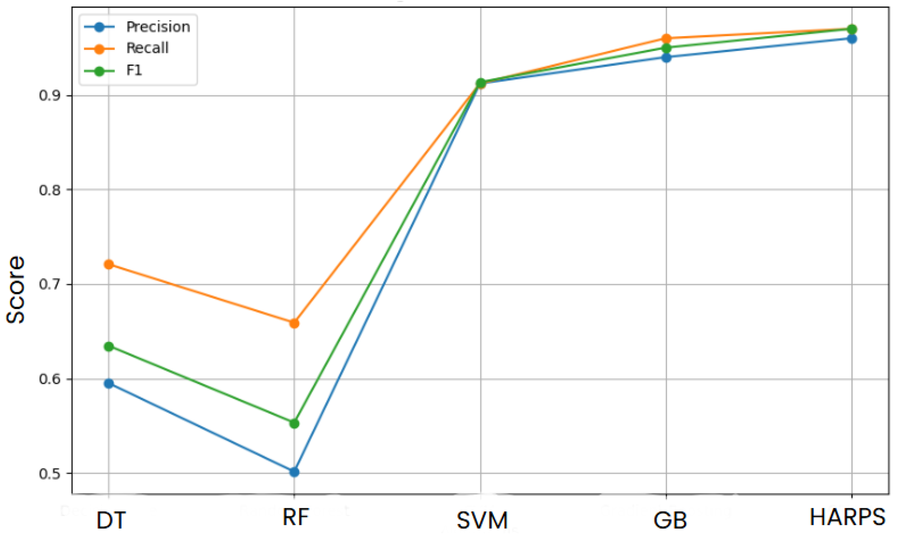
Based on three important metrics, the precision, recall and the F1 score in Figure 5 offer a perceptive look at how different ML algorithms perform compared to each other on a dataset.

The DT algorithm, the simplest of the algorithms tested, clearly performs poorly on this particular dataset, with the lowest scores across all criteria. Decision trees may overfit training data, leading to poor generalization on unseen data, which could be the source of this.

The SVM algorithm’s performance is comparable to that of the RF, indicating that its strategy of identifying the best hyperplane for classification works effectively with this dataset. SVMs succeed at managing datasets with a large number of features, and their effectiveness in this high-dimensional space may be attributed to their capacity to operate in this environment.

GB improves performance, refining slightly in this evaluation compared to SVM and RF. It concentrates on hard circumstances that previous models misclassified, potentially increasing accuracy, by creating trees sequentially and having each tree attempt to correct the errors of the previous one.

Finally, the HARPS algorithm exhibits a combination of the attributes of the previous four algorithms and seems to be a personalized hybrid model, based on its leading outcomes. This implies that HARPS might be using the robustness of RF, the iterative improvement method of GB, and the dimensionality-handling capacity of SVMs. This could capture more data patterns and correlations, leading to better precision, recall, and F1 scores. The hybrid approach in question likely aims to take advantage of the unique benefits of each base algorithm, producing a very flexible and reliable model that performs well in various dataset dimensions. This performance could be especially helpful in real-world situations when it is necessary to strike a balance between various types of errors.

6. Conclusions

ML approaches are an overwhelming choice for researchers to extract valuable insights from huge datasets, specifically in the field of plant stresses. There is significant improvement in how ML classification algorithms are developed and validated, using larger and more diverse data sets. A novel framework called the Hybrid Algorithm for Robust Plant Stress (HARPS) is proposed in this research. The results depict that the proposed algorithm HARPS outperforms existing approaches with an accuracy of 96.6% and a processing time of only 8 s. HARPS’s fast processing speed and high precision make it a perfect choice for many applications in future, like smart farming and smart health systems. In addition to its technical capabilities, HARPS contributes significantly to sustainable agriculture. The framework minimizes unnecessary utilization of chemical treatments, maximizes resource inputs like fertilizer and water, and promotes the development of crop types that are climate robust by making it easier to identify stress in crops early and accurately. This results in more flexible, data-driven crop management techniques, increased agricultural output, and lower adverse environmental effects.

References

1. Erenstein, O.; Jaleta, M.; Mottaleb, K.A.; Sonder, K.; Donovan, J.; Braun, H.J. Global trends in wheat production, consumption and trade. In Wheat Improvement: Food Security in a Changing Climate; Springer International Publishing: Cham, Switzerland, 2022; pp. 47–66. [Google Scholar]
2. Wing, I.S.; De Cian, E.; Mistry, M.N. Global vulnerability of crop yields to climate change. J. Environ. Econ. Manag. 2021, 109, 102462. [Google Scholar] [CrossRef]
3. Rehman, M.U.; Eesaar, H.; Abbas, Z.; Seneviratne, L.; Hussain, I.; Chong, K.T. Advanced drone-based weed detection using feature-enriched deep learning approach. Knowl.-Based Syst. 2024, 305, 112655. [Google Scholar] [CrossRef]
4. Farooq, M.; Frei, M.; Zeibig, F.; Pantha, S.; Özkan, H.; Kilian, B.; Siddique, K.H. Back into the wild: Harnessing the power of wheat wild relatives for future crop and food security. J. Exp. Bot. 2025, eraf141. [Google Scholar] [CrossRef] [PubMed]
5. Muthuramalingam, P.; Jeyasri, R.; Selvaraj, A.; Kalaiyarasi, D.; Aruni, W.; Pandian, S.T.K.; Ramesh, M. Global transcriptome analysis of novel stress associated protein (SAP) genes expression dynamism of combined abiotic stresses in Oryza sativa (L.). J. Biomol. Struct. Dyn. 2021, 39, 2106–2117. [Google Scholar] [CrossRef]
6. Zahravi, M.; Amirbakhtiar, N.; Arhsad, Y.; Mahdavimajd, J. Identifying key traits for heat stress tolerance in wheat using machine learning. Iran. J. Genet. Plant Breed. 2024, 13, 61–84. [Google Scholar]
7. Sharma, N.; Kumar, M.; Daetwyler, H.D.; Trethowan, R.M.; Hayden, M.; Kant, S. Phenotyping for heat stress tolerance in wheat population using physiological traits, multispectral imagery, and machine learning approaches. Plant Stress 2024, 14, 100593. [Google Scholar] [CrossRef]
8. Wang, L.; Zhang, H.; Bian, L.; Zhou, L.; Wang, S.; Ge, Y. Poplar seedling varieties and drought stress classification based on multi-source, time-series data and deep learning. Ind. Crops Prod. 2024, 218, 118905. [Google Scholar] [CrossRef]
9. Chandel, N.S.; Rajwade, Y.A.; Dubey, K.; Chandel, A.K.; Subeesh, A.; Tiwari, M.K. Water stress identification of winter wheat crop with state-of-the-art AI techniques and high-resolution thermal-RGB imagery. Plants 2022, 11, 3344. [Google Scholar] [CrossRef]
10. Jeyasri, R.; Muthuramalingam, P.; Satish, L.; Pandian, S.K.; Chen, J.-T.; Ahmar, S.; Wang, X.; Mora-Poblete, F.; Ramesh, M. An overview of abiotic stress in cereal crops: Negative impacts, regulation, biotechnology and integrated omics. Plants 2021, 10, 1472. [Google Scholar] [CrossRef]
11. Xu, L.; Zhu, X.; Yi, F.; Liu, Y.; Sod, B.; Li, M.; Chen, L.; Kang, J.; Yang, Q.; Long, R. A genome-wide study of the lipoxygenase gene families in Medicago truncatula and Medicago sativa reveals that MtLOX24 participates in the methyl jasmonate response. BMC Genom. 2024, 25, 195. [Google Scholar] [CrossRef]
12. Madani, A.; Krause, B.; Greene, E.R.; Subramanian, S.; Mohr, B.P.; Holton, J.M.; Olmos, J.L., Jr.; Xiong, C.; Sun, Z.Z.; Socher, R.; et al. Large language models generate functional protein sequences across diverse families. Nat. Biotechnol. 2023, 41, 1099–1106. [Google Scholar] [CrossRef] [PubMed]
13. Perez, J.J.; Perez, R.A.; Perez, A. Computational modeling as a tool to investigate PPI: From drug design to tissue engineering. Front. Mol. Biosci. 2021, 8, 681617. [Google Scholar] [CrossRef] [PubMed]
14. Abbas, Z.; Kim, S.; Lee, N.; Kazmi, S.A.W.; Lee, S.W. A robust ensemble framework for anticancer peptide classification using multi-model voting approach. Comput. Biol. Med. 2025, 188, 109750. [Google Scholar] [CrossRef] [PubMed]
15. Miller, C.; Portlock, T.; Nyaga, D.M.; O’Sullivan, J.M. A review of model evaluation metrics for machine learning in genetics and genomics. Front. Bioinform. 2024, 4, 1457619. [Google Scholar] [CrossRef]
16. Niu, Y.; Han, W.; Zhang, H.; Zhang, L.; Chen, H. Estimating fractional vegetation cover of maize under water stress from UAV multispectral imagery using machine learning algorithms. Comput. Electron. Agric. 2021, 189, 106414. [Google Scholar] [CrossRef]
17. Smith, J.; Johnson, A. Application of Artificial Intelligence in Assessing Plant Stress: A Comprehensive Review. J. Agric. Sci. 2023, 76, 210–225. [Google Scholar]
18. Hastie, T.; Tibshirani, R.; Friedman, J. The Elements of Statistical Learning; Springer: New York, NY, USA, 2009. [Google Scholar]
19. Mitchell, T.M. Machine Learning; McGraw-Hill: New York, NY, USA, 1997. [Google Scholar]
20. Rigatti, S.J. Random Forest. J. Insur. Med. 2017, 47, 31–39. [Google Scholar] [CrossRef]
21. Biau, G.; Scornet, E. A random forest guided tour. Test 2016, 25, 197–227. [Google Scholar] [CrossRef]
22. Abe, S. Support Vector Machines for Pattern Classification; Springer: Berlin/Heidelberg, Germany, 2005. [Google Scholar]
23. Amarappa, S.; Sathyanarayana, S.V. Data classification using Support Vector Machine (SVM), a simplified approach. Int. J. Electron. Comput. Sci. Eng 2014, 3, 435–445. [Google Scholar]
24. Friedman, J. Greedy function approximation: A gradient boosting machine. Ann. Stat. 2001, 29, 1189–1232. [Google Scholar] [CrossRef]
25. Mustafa, O.M.; Ahmed, O.M.; Saeed, V.A. Comparative Analysis of Decision Tree Algorithms Using Gini and Entropy Criteria on the Forest Covertypes Dataset. In Proceedings of the The International Conference on Innovations in Computing Research; Springer: Cham, Switzerland, 2024; pp. 185–193. [Google Scholar]
26. Bukhori, H.A.; Munir, R. Inductive Link Prediction Banking Fraud Detection System Using Homogeneous Graph-Based Machine Learning Model. In Proceedings of the 2023 IEEE 13th Annual Computing and Communication Workshop and Conference (CCWC), Virtual, 8–11 March 2023; pp. 0246–0251. [Google Scholar] [CrossRef]
27. Chernozhukov, V.; Chetverikov, D.; Kato, K.; Koike, Y. High-Dimensional Data Bootstrap. Annu. Rev. Stat. Its Appl. 2023, 10, 427–449. [Google Scholar] [CrossRef]
28. Afkham, B.M.; Chung, J.; Chung, M. Learning Regularization Parameters of Inverse Problems via Deep Neural Networks. Inverse Probl. 2021, 37, 105017. [Google Scholar] [CrossRef]
29. Ghojogh, B.; Ghodsi, A.; Karray, F.; Crowley, M. Reproducing Kernel Hilbert Space, Mercer’s Theorem, Eigenfunctions, Nyström Method, and Use of Kernels in Machine Learning: Tutorial and Survey. arXiv 2021, arXiv:2106.08443. [Google Scholar] [CrossRef]
30. Granziol, D.; Zohren, S.; Roberts, S. Learning Rates as a Function of Batch Size: A Random Matrix Theory Approach to Neural Network Training. J. Mach. Learn. Res. 2022, 23, 1–65. [Google Scholar]
31. Letunic, I.; Khedkar, S.; Bork, P. SMART: Recent Updates, New Developments and Status in 2020. Nucleic Acids Res. 2021, 49, D458–D460. [Google Scholar] [CrossRef]
32. Mistry, J.; Chuguransky, S.; Williams, L.; Qureshi, M.; Salazar, G.A.; Sonnhammer, E.L.L.; Tosatto, S.C.E.; Paladin, L.; Raj, S.; Richardson, L.J.; et al. Pfam: The protein families database in 2021. Nucleic Acids Res. 2021, 49, D412–D419. [Google Scholar] [CrossRef]
33. Larralde, M.; Zeller, G. PyHMMER: A Python library binding to HMMER for efficient sequence analysis. Bioinformatics 2023, 39, btad214. [Google Scholar] [CrossRef]
34. The UniProt Consortium. UniProt: The Universal Protein Knowledgebase in 2021. Nucleic Acids Res. 2021, 49, D480–D489. [Google Scholar] [CrossRef]
35. Coudert, E.; Gehant, S.; de Castro, E.; Pozzato, M.; Baratin, D.; Neto, T.; Sigrist, C.J.A.; Redaschi, N.; Bridge, A.; The UniProt Consortium. Annotation of biologically relevant ligands in UniProtKB using ChEBI. Bioinformatics 2023, 39, btac793. [Google Scholar] [CrossRef]
36. Schroeder, L.; Krepl, M.; Pumplin, N. Protein pI influences solubility and heat stability during stress. J. Plant Physiol. 2020, 251, 153243. [Google Scholar]
37. Yang, W.; Wu, X.; Li, Z. Molecular weight and protein folding mechanisms in heat stress conditions. J. Mol. Biol. 2021, 433, 167112. [Google Scholar]
38. Haider, S.; Iqbal, J.; Naseer, S.; Yaseen, T.; Shaukat, M.; Bibi, H.; Mahmood, T. Molecular mechanisms of plant tolerance to heat stress: Current landscape and future perspectives. Plant Cell Rep. 2021, 40, 2247–2271. [Google Scholar] [CrossRef] [PubMed]
39. Tsuboyama, K.; Osaki, T.; Matsuura-Suzuki, E.; Kozuka-Hata, H.; Okada, Y.; Oyama, M.; Tomari, Y. A widespread family of heat-resistant obscure (Hero) proteins protect against protein instability and aggregation. PLoS Biol. 2020, 18, e3000632. [Google Scholar] [CrossRef] [PubMed]
40. Blaabjerg, L.M.; Kassem, M.M.; Good, L.L.; Jonsson, N.; Cagiada, M.; Johansson, K.E.; Lindorff-Larsen, K. Rapid protein stability prediction using deep learning representations. Elife 2023, 12, e82593. [Google Scholar] [CrossRef] [PubMed]
Figure 1. Hybrid Algorithm for Robust Plant Stress (HARPS).
Sustainability 17 05767 g001
Figure 2. From raw information to informed decisions, witness the path of ML Classification.
Sustainability 17 05767 g002
Figure 3. Analysis of molecular weight, theoretical pI and instability index in terms of Uniport ID.
Sustainability 17 05767 g003
Figure 4. Results of ablation analysis using 80% of the data for training.
Sustainability 17 05767 g004
Figure 5. Performance comparison in terms of Precision, Recall and F1 Measures.
Sustainability 17 05767 g005