1. Introduction
Coordinated advancement of high-quality financial growth and urban–rural economic integration serves as a crucial solution to China’s urban–rural development imbalance and forms a foundation for establishing the new dual-circulation development paradigm. Currently, the factor mismatch, industrial disconnection, and livelihood gap caused by the binary division of the urban and rural economies has become the core short board that restricts sustainable economic growth. In response, the National Development and Reform Commission released the Urban–Rural Economic Integration Strategy in 2022, emphasizing infrastructure extension to rural areas using counties as foundational units. Therefore, urban–rural economic integration must be treated as a strategic priority.
As the financial system is the hub of resource allocation, high-quality finance development encompasses a clear understanding of the fundamental nature and functions of the financial sector, the construction of a modern institutional framework, the refinement of organizational structures, and the improvement of service efficiency (Sun Jun et al., 2020) [
1]. A robust financial system can catalyze factor mobility, stimulate rural revitalization, and energize new urbanization. However, challenges such as the traditional financial system’s misalignment with county-level economies, underdeveloped rural financial infrastructure, and limited urban–rural capital flow persist. To overcome these barriers, reforms and technological innovations are urgently needed. On the one hand, high-quality finance must emphasize the synergistic integration of inclusive, green, and digital finance. This includes developing tailored policy instruments and multi-tiered capital markets to direct financial resources toward rural agriculture and small enterprises, fostering deeper integration between industrial and financial chains. On the other hand, urban–rural economic integration demands enhanced industrial coordination, consumer market upgrading, and digital governance to dismantle institutional and geographic divides and facilitate the bi-directional flow of talent, capital, and technology. The deep coupling of the two requires the financial system to optimize its functional layout in order to serve the entities and also requires the process of urban–rural integration to use financial empowerment as a lever to support the endogenous momentum. Through institutional synergy and technology-driven and ecological co-construction, promoting the “two-way running to” of finance and urban–rural development will provide a systematic solution for high-quality development under the goal of common prosperity. Therefore, this paper aims to use the coupling coordination model to test the degree of coupling and coordination between the two and explore the influencing mechanism of the deep integration of the two under the goal of common prosperity.
This paper examines how high-quality financial development interacts with urban–rural economic integration by utilizing Chinese provincial panel data from 2011 to 2022. The marginal contributions include the following: (1) in the study of urban–rural economic integration, the concept of financial high-quality development is introduced for the first time and the relationship between financial high-quality development and urban–rural economic integration is explored in depth; (2) the degree of coupled and coordinated development of the two, regional differences, and spatial correlation are analyzed in depth by using econometric models, such as the Gini coefficient method; (3) the influencing factors of the coordinated interaction between the two systems are investigated in depth, which provides references to the government’s efforts in promoting the coupled and coordinated development of the two. It provides reference for the government to promote the coordinated development of the two.
Existing literature on urban–rural economic integration remains relatively underdeveloped, with most research centering on the broader theme of urban–rural integration.
- (1)
Definitions and conceptual boundaries: At present, there is no universally accepted method for evaluating the extent of urban–rural integration. Some scholars suggest that it can be examined through key dimensions such as the movement of production factors, the growth of industries, infrastructure development, and access to public services (Yang et al., 2021) [
2]. Others propose that the concept should be expanded to encompass multiple layers, including economic, spatial, and social integration—such as the merging of urban and rural economies, labor and capital flows, student exchanges, and coordinated spatial development—alongside the equitable distribution of development benefits (Ma et al., 2020; He et al., 2019) [
3,
4]. Existing literature focuses on the overall measurement of urban–rural integration, but does not involve the measurement of urban–rural economic integration as an important part of urban–rural integration.
- (2)
Influencing factors. Bah et al. (2007) [
5] found that government initiatives to provide subsidies for transportation facilities can improve transportation connectivity and enhance urban–rural economic integration. Sharma (2017) [
6] argued that worker commuting can help to narrow the urban–rural gap and promote urban–rural economic integration. Forero (2013) [
7] and Zhang (2023) [
8] found that the platform economy, as a new type of data-driven, platform-supported, and network-synergized economic system, provides a new impetus for the development of urban–rural integration. Nguyen et al. (2020) [
9] argued for the specific impact of international integration on the urban–rural income gap. Yang et al. (2021) [
10] found that the transformation of rural land use can effectively promote urban–rural integration. According to Tan et al. (2023) [
11], tourism plays a key role in promoting urban–rural integration, although its effectiveness declines as economic development matures. Yin and Wang (2022) [
12] pointed out that the digital economy contributes to integration by easing disparities in capital flow and data allocation between urban and rural regions.
There is limited research specifically targeting the intersection of high-quality financial development and urban–rural economic integration. Existing literature tends to emphasize a few key dimensions. (1) Financial development and urban–rural residents’ income. For instance, Su et al. (2019) [
13] found that financial progress in rural areas, based on bootstrap Granger panel causality tests, can boost rural incomes and reduce disparities. Similarly, Yu and Wang (2021) [
14] showed that digital inclusive finance helps to bridge income gaps by addressing inequalities in wages and property income. Ji et al. (2021) [
15] also emphasized that inclusive finance, by expanding access and reducing financial exclusion, can help to narrow the rural–urban income divide.
In contrast, some studies point to potential adverse effects. Tiwari et al. (2013) [
16], using an ARDL bounds test, concluded that financial development, when combined with economic growth and inflation, may worsen income inequality. Wu et al. (2020) [
17] suggested that inclusive finance may have limited effectiveness, and Ye et al. (2023) [
18], employing a GMM framework, found that rising financial development levels might further increase income disparities. Moreover, Su et al. (2019) [
13] proposed a nonlinear dynamic, observing an inverted U-shaped relationship where initial financial growth increases the income gap before eventually narrowing it. Huang and Zhang (2020) [
19], applying a panel cointegration approach, concluded that financial development tends to widen income disparities in the short term while reducing them in the long run.
- (3)
Financial development and urban economy. Wong et al. (2021) [
20] analyzed and found that the spatial agglomeration of the financial services industry contributes significantly to the quality of urban economic growth. Li et al. (2022) [
21] argued that digital inclusive finance can promote urban innovation through improving the allocation of credit resources, consumption, and industrial upgrading, which in turn promotes the development of the urban economy. Li et al. (2023) [
22] and Sun and You (2023) [
23] found that digital inclusive finance significantly enhances the economic vitality of urban areas, with improving innovation and entrepreneurship and stimulating consumption as important paths.
- (4)
Agricultural development and rural poverty reduction. Odhiambo (2010) [
24] found a significant causal relationship between financial development and rural poverty reduction. Ajide (2015) [
25] and Olaniyi (2017) [
26] found that financial inclusion has a positive impact on rural poverty reduction, but is mitigated or even offset by borrowing costs and financial openness. Wang and Kou (2017) [
27] argue that the development of rural financial institutions can effectively solve the financing problems in agricultural production, rural health and old-age care, boutique housing development, and the construction of tourism facilities, and is conducive to the promotion of high-economic-value-added service-oriented agriculture. Gautam et al. (2022) [
28] argue that regional village banks have a favorable poverty reduction and rural development impact. Wang et al. (2022) [
29] found that financial penetration can effectively boost economic growth in rural areas, which in turn accelerates rural poverty alleviation. Yang and Ma (2022) [
30] found that from the perspectives of the income growth effect and vulnerability mitigation effect digital financial inclusion can not only improve rural residents’ entrepreneurship and wage income by increasing their entrepreneurship and wage income, but also mitigate exogenous shocks through mitigating the effects to reduce the uncertainty of rural residents’ future income.
To summarize, existing research focuses on the influencing factors of urban–rural economic integration, including transportation facilities, workers’ commuting, platform economy, etc., and also focuses on the impact of financial development on urban and rural residents’ income, the urban and rural economy, agricultural development, and rural poverty reduction. There are few studies that integrate high-quality financial development into urban–rural economic integration, and there is no literature focusing on the degree of coupling and coordination between high-quality financial development and urban–rural economic integration. Therefore, this paper constructs a quantitative model to test the degree of coupling and coordination between the two and the influencing factors.
2. Mechanism of Action
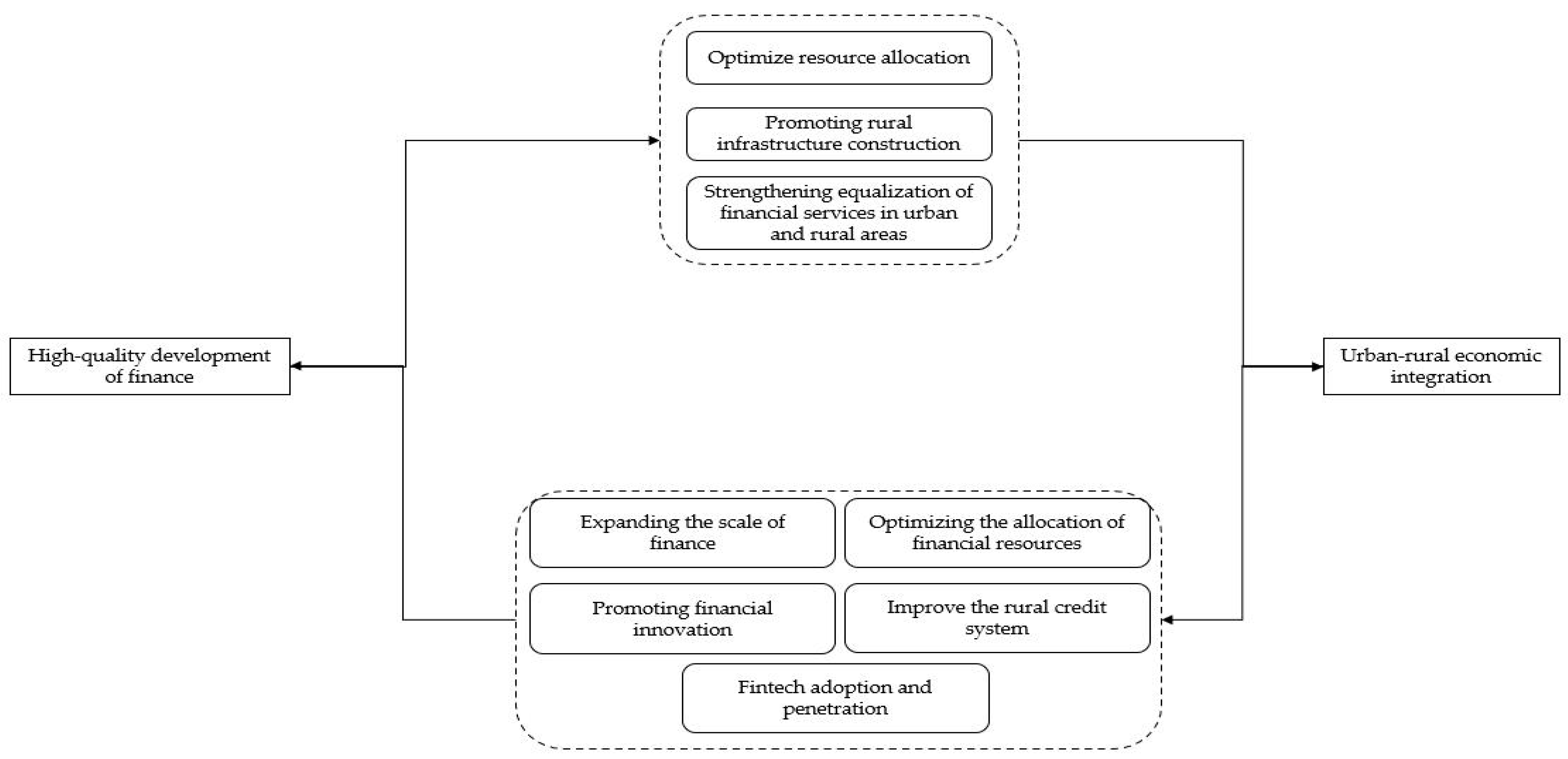
We believe that high-quality financial development and urban–rural economic integration complement each other (see
Figure 1).
High-quality financial development provides a strong impetus for urban–rural economic integration. This paper argues that high-quality financial development can promote urban–rural economic integration through such paths as optimizing resource allocation, advancing rural infrastructure construction, and strengthening the equalization of urban and rural financial services. First, the high-quality financial system can effectively guide the flow of funds to the rural development of potential industry, support new agricultural business entities to expand their scale, introduce advanced technology, promote the upgrading of rural industry, and enhance the strength of the rural economic development through accurate risk assessment and investment decisions (Qi et al., 2024) [
31]. Second, financial institutions, with the help of issuing bonds and setting up funds, have guided social capital to participate in the construction of rural roads, communications, and other infrastructure, improved the logistics and distribution system, reduced transportation costs, and promoted the circulation of urban and rural commodities (Ge et al., 2022) [
32]. Third, high-quality financial development also improves the level of rural financial risk management and promotes the equalization of financial services. Financial institutions have increased their investment in rural financial resources to enhance service coverage, while providing diversified risk management tools to help rural enterprises and farmers stabilize business income and reduce risks (Hao Ying et al., 2023) [
33].
Rural–urban economic integration promotes high-quality financial development through multiple mechanisms. Firstly, urban–rural economic integration can promote the high-quality development of finance by expanding the financial scale. Urban–rural economic integration implies the rapid development of the rural economy and the continuous expansion of the rural consumer market, which makes the consumption of rural residents increasingly diversified (Liu et al., 2016) [
34] and drives the growth of demand for financial services, thus expanding the scale of the financial market and creating more business opportunities for financial institutions. Secondly, urban–rural economic integration helps to achieve the optimal allocation of financial assets and promotes high-quality financial development. Urban–rural economic integration constantly optimizes the rural industrial structure, gives rise to new industries and business models, provides more high-quality investment projects for financial institutions, prompts them to reasonably allocate assets, reduces risks, improves returns, and thus achieves high-quality financial development (Liu, 2022) [
35]. In addition, urban–rural economic integration can also promote financial innovation and financial high-quality development. Urban–rural economic integration promotes the emergence of new economic models and transaction methods, forcing the innovation of financial products and services to meet the diversified financial needs in the process of urban–rural integration (Liu et al., 2021) [
36]. Finally, urban–rural integration contributes to a healthier financial ecosystem by reinforcing rural credit systems, raising awareness of credit practices, and fostering a more transparent and equitable market environment. It also enhances the application and reach of financial technologies in rural regions, accelerating both their adoption and the overall quality of financial services (Zhan et al., 2023) [
37].
3. Research Design
3.1. Variable
- (1)
Urban–rural economic integration (ECO).
Referring to the research methods of Muga et al. (2023) [
38] and Tan et al. (2023) [
11], eight specific indicators are selected to construct an index system to evaluate the urban–rural economic integration from six different dimensions, namely, economic aggregate, industrial structure, financial structure, employment structure, income structure, and consumption structure (see
Table 1).
- (2)
Financial high-quality development index (AFIN).
Since there are fewer studies on financial high-quality development, this paper draws on the research ideas of Wang et al. (2018) [
39] and Li et al. (2020) [
40] and combines data availability to construct a financial high-quality development index system by selecting 15 indexes from the perspectives of the six dimensions of the overall innovation, openness, greenness, coordination, and sharing (see
Table 2).
- (3)
Data source and processing
Given the unavailability of data for Tibet, Taiwan, Hong Kong, and Macau, this study focuses on a panel dataset comprising 30 Chinese provinces from 2011 to 2022, to assess the coupling coordination between high-quality financial development and urban–rural economic integration (Liu et al., 2022) [
41]. Data for financial inclusion indicators—specifically usage depth and coverage breadth—are sourced from the Peking University Digital Financial Inclusion Index. The financial efficiency metric is derived using the SBM model, incorporating inputs such as the number of financial institutions, industry employment, and fixed asset investment, with the output being the value added by the financial sector, based on data from the Wind database. Additional indicators are collected from the China Statistical Yearbook and China Rural Statistical Yearbook (2011–2022). For urban–rural integration variables, figures on industry output and employment come from the China Population and Employment Statistical Yearbook, while the remaining data are drawn from the China Statistical Yearbook.
3.2. Modeling and Research Methods
3.2.1. Entropy Value Method
As an objective weighting method, the entropy weight method determines the weight of each indicator by quantifying the discrete degree of the indicator, effectively reducing subjective interference and objectively reflecting the degree of variation between indicators. Therefore, this paper uses the entropy weight method to measure the development level of the two. The specific steps are as follows:
- (1)
Data standardization through the following equations:
where in Equations (1) and (2)
i denotes provinces,
t denotes time, and
j denotes specific indicators. After normalizing the data for all indicators, the weights assigned to each indicator need to be further calculated.
- (2)
Calculation of the weights assigned to each indicator using the following equation:
- (3)
Calculate the information entropy value of the jth metric as well as the information entropy redundancy. Where k = 1/ln(n) while satisfying e > 0 in the following equation:
- (4)
Calculate the information entropy redundancy through the following equation:
- (5)
Calculate the weights of the indicators and calculate the composite score through the following equations:
3.2.2. Coupled Coordination Model
Following the approaches of Shi et al. (2020) [
42], this study develops a coupling coordination model to evaluate the relationship between high-quality financial development and urban–rural economic integration at the provincial level. The model is as follows:
where
AFIN and
ECO denote the indicators of high-quality financial development and urban–rural economic integration, respectively, and
C denotes the degree of coupling of the two systems. In order to further analyze the degree of coordination of the two systems, the coupled coordination model as follows is used to explore the specific model:
where
T represents the overall evaluation index, while
D denotes the degree of coordinated development between the two systems. Drawing on the research of Wang et al. (2023) [
43], we believe that the development indexes of the two are equally important, so the weights
α and
β are both set at 0.5. And the degree of coupling coordination is classified into distinct levels, as outlined in
Table 3.
3.2.3. Dagum’s Gini Coefficient
This study adopts the methodology proposed by Tao et al. (2023) [
44] to examine the disparities in it. Specifically, the Gini coefficient is employed to quantify the overall variation and identify its underlying sources, with calculations based on the following formula:
where
G represents the overall Gini coefficient; k is the number of regional groups; n refers to the total number of provinces;
yij(
yhr) indicates the coordination level of provinces within region
j(
h); and the symbol
denotes the average coordination score across 30 provinces. A higher Gini value reflects greater imbalance in the degree of rural revitalization.
The Dagum Gini coefficient can be decomposed into intra-region variance
Gω, inter-region variance
Gnb, and hypervariance density
Gt, calculated as follows:
where
Gjj is the intra-regional variation,
Gω is the intra-regional variation contribution, and
nj is the number of provinces within the
jth region. Furthermore,
and
. The following equations are also used:
where
Gjh is the inter-district variance and
Gnb is the inter-district contribution to the variance.
,
, and
Djh is the relative impact of the coupling harmonization between the
jth,
hth region. Therefore, the following equation is used:
where
Gt is the hypervariable density contribution.
3.2.4. Kernel Density Method
Based on the approach of Lv et al. (2021) [
45], this study employs the kernel density estimation technique to explore the temporal evolution of coupling coordination. As a nonparametric method, it captures changes in random variables over time to illustrate the distribution trends of regional differences. The corresponding formula is as follows:
where
N is the number of samples,
h is the bandwidth,
Xi is the independent identically distributed observations,
x is the mean, and
K (·) denotes the kernel function.
3.2.5. Spatial Autocorrelation Model
To assess the spatial linkage in the coordinated development of the two, this study applies the
Moran’s I index. The global
Moran’s I evaluates overall spatial clustering across regions, while the local
Moran’s I identifies specific areas and intensities of spatial association. The respective formulas for both indices are presented below:
where
n represents 30 provinces,
yi is the coupling coordination degree between high-quality financial development and urban–rural economic integration in province
I,
y0 is the average value of the coupling coordination degree between high-quality financial development and urban–rural economic integration, and
wij represents the elements in the spatial weight matrix.
4. Empirical Analysis
4.1. Analysis of High-Quality Financial Development and the Level of Urban–Rural Economic Integration
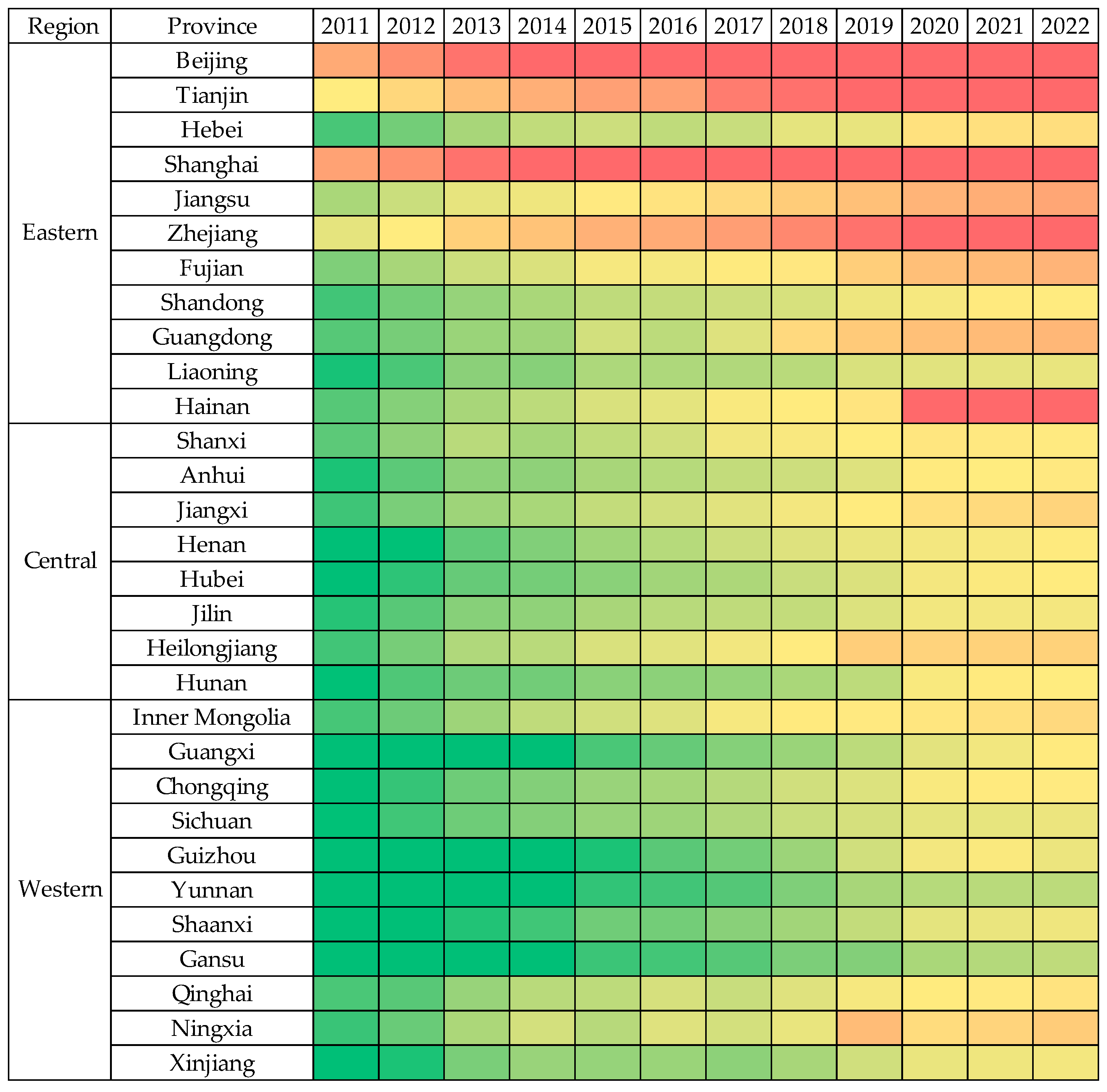
Table 4 presents regional data on financial quality development and urban–rural economic integration for 2011 and 2022. The results reveal a notable improvement in both dimensions across all provinces over the period. This progress can be attributed to the following two main factors: first, ongoing financial reforms have shifted regional priorities toward comprehensive financial modernization, driving steady enhancements in financial system quality; second, the rollout of urban–rural integration policies has laid a solid groundwork for fostering closer economic ties between urban and rural areas.
Between 2011 and 2022, the growth trajectories of high-quality financial development varied among provinces, but distinct regional disparities remained—most notably, the persistent pattern of “strong in the east and weak in the west”. A similar trend is observed in urban–rural economic integration. In 2011, provinces such as Guizhou, Gansu, Guangxi, Yunnan, and Qinghai exhibited the lowest integration levels, while Beijing, Shanghai, and Tianjin led the rankings. By 2022, Guizhou, Gansu, Yunnan, Shaanxi, and Jilin remained among the lowest performers, whereas Beijing, Shanghai, Tianjin, Zhejiang, and Jiangsu continued to dominate. This is mainly due to the strong economic strength, sound industrial system, active policy innovation, and high level of integration of urban and rural infrastructure and public services in these regions, which has promoted the efficient flow and integrated development of urban and rural factors. These patterns underscore the enduring regional imbalance in both financial development and economic integration, with the eastern region maintaining a clear advantage.
4.2. Systematic Coupling Time Analysis of Financial High-Quality Development and Urban–Rural Economic Integration
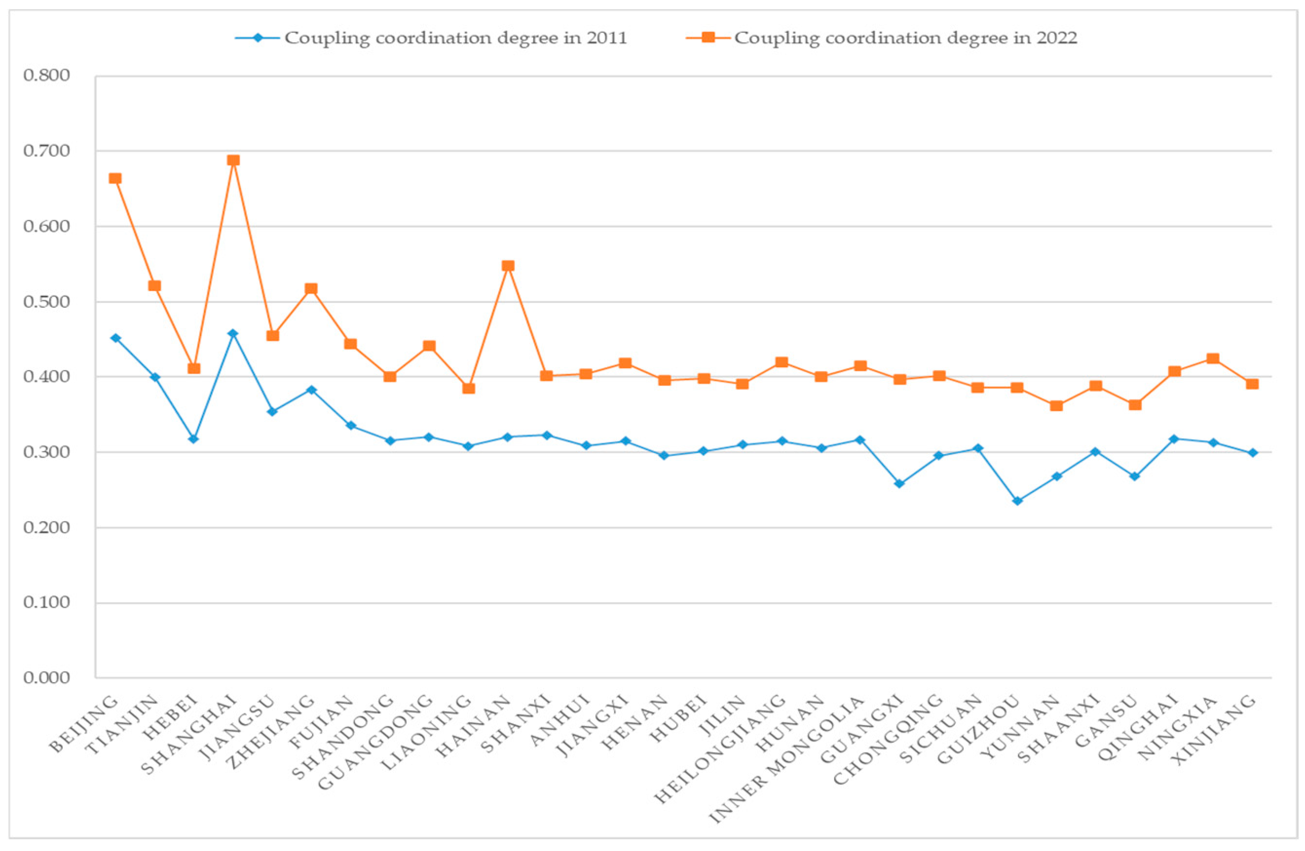
Based on the line graph depicting provincial coupling coordination degrees in 2011 and 2022 (see
Figure 2), it is evident that most provinces experienced an upward trend by 2022. This suggests a steady enhancement in the integration between high-quality financial development and urban–rural economic growth over time. Despite this progress, the overall coordination level remains relatively low nationwide, with notable regional disparities (See
Figure 3). In
Figure 3, Provinces like Beijing and Shanghai exhibit the strongest synergy between the two systems, while Gansu and Yunnan remain at the lower end of the spectrum.
As shown in
Table 5, the national average of the coupling coordination degree between financial high-quality development and urban–rural economic integration exhibited a steady upward trend from 2011 to 2022. However, by 2022, the coupling coordination level is 0.434, which is lower than 0.5 and is on the verge of disharmony. Regarding regional growth, the eastern region recorded the highest increase (0.137), followed by the western (0.104) and central (0.095) regions, with only the eastern area surpassing the national average growth rate of 0.113. Furthermore, the data from 2011 to 2022 confirm pronounced regional disparities, with the eastern provinces consistently achieving the highest coordination levels and the western provinces lagging behind in both the degree and rate of improvement. The possible reasons are that the eastern region has a strong economic foundation, abundant financial resources, sound systems, and obvious advantages in infrastructure and human capital, which promote the coordinated development of financial and urban–rural integration; meanwhile the western region lags behind in development, has insufficient resources, and weak service capabilities, resulting in a low level of coupling and coordination.
4.3. Dynamic Study of Coupling Coordination Degree
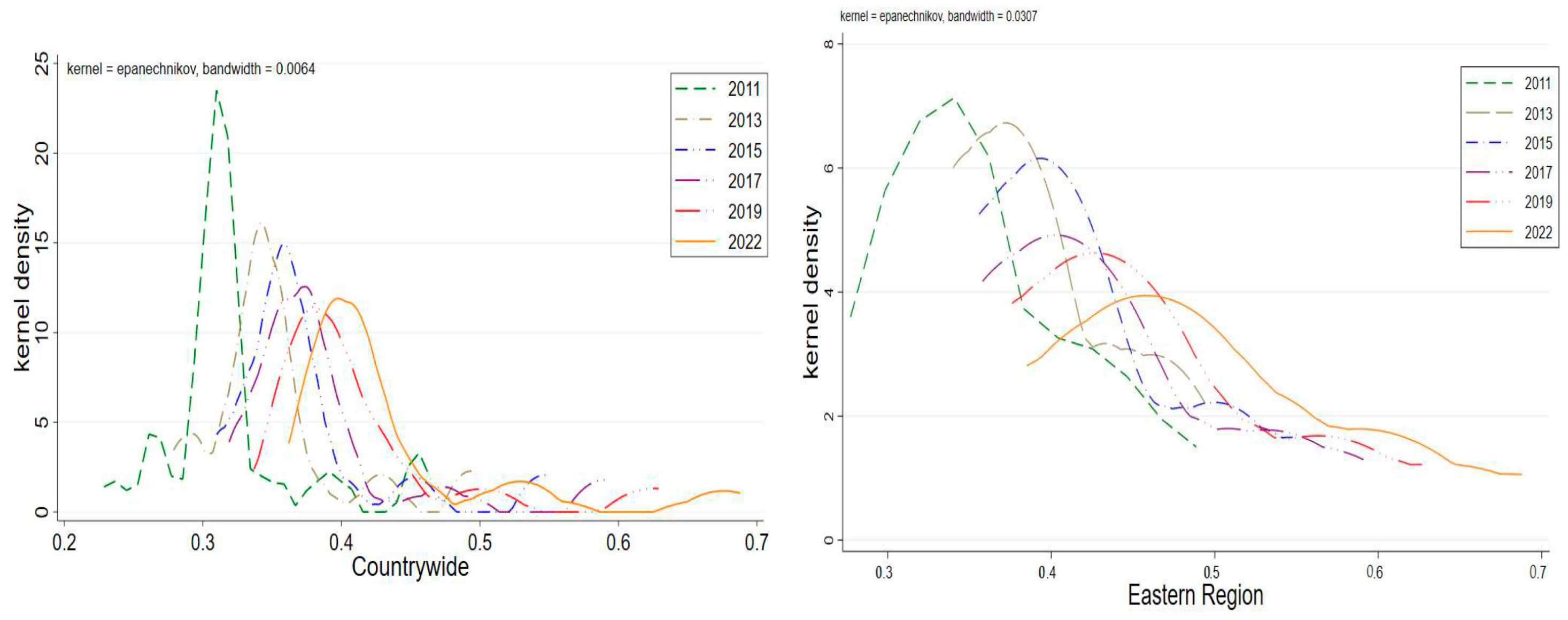
This study uses the years 2011, 2014, 2017, and 2022 as reference points and employs Gaussian kernel density estimation to analyze the distribution of the coupling coordination levels at the national level as well as in the eastern, central, and western regions. Detailed results are presented in
Figure 4.
National region: The national kernel density curve exhibits a rightward shift with minor amplitude, indicating a consistent upward trajectory in the coupling coordination degree between financial development and urban–rural integration. Its multi-peak structure—featuring a dominant peak alongside secondary ones—suggests the presence of polarization in development levels. Meanwhile, the declining height and expanding width of the main peak, along with a noticeable rightward skew, point to widening disparities and a stepwise distribution trend.
Eastern region: The density curve moves markedly to the right, reflecting a strong growth momentum. The distribution is predominantly single-peaked, suggesting relatively uniform advancement across provinces with minimal polarization. However, the declining peak height, increasing curve width, and evident right-tail drag highlight substantial internal differences and a pronounced tiered structure.
Central region: The central area’s density curve also shifts rightward, showing a faster rise in coordination levels. Initially characterized by multiple peaks, the distribution transitions to a more unified single-peak form over time, indicating diminishing polarization. The curve’s peak height first declines and then rises, while its width follows a “narrow–wide–narrow” sequence. Though overall differences remain notable, internal disparities are gradually converging, with the right skew effect weakening.
Western region: The western region’s curve similarly trends rightward, marking steady improvement. The multi-peak structure seen in earlier years diminishes, giving way to a dominant single-peak—evidence that polarization is subsiding. The increasing peak height and narrowing distribution width, coupled with the absence of strong right-tail drag, indicate that inter-provincial gaps are narrowing.
4.4. Regional Differences and Decomposition of Coupling Coordination Degree
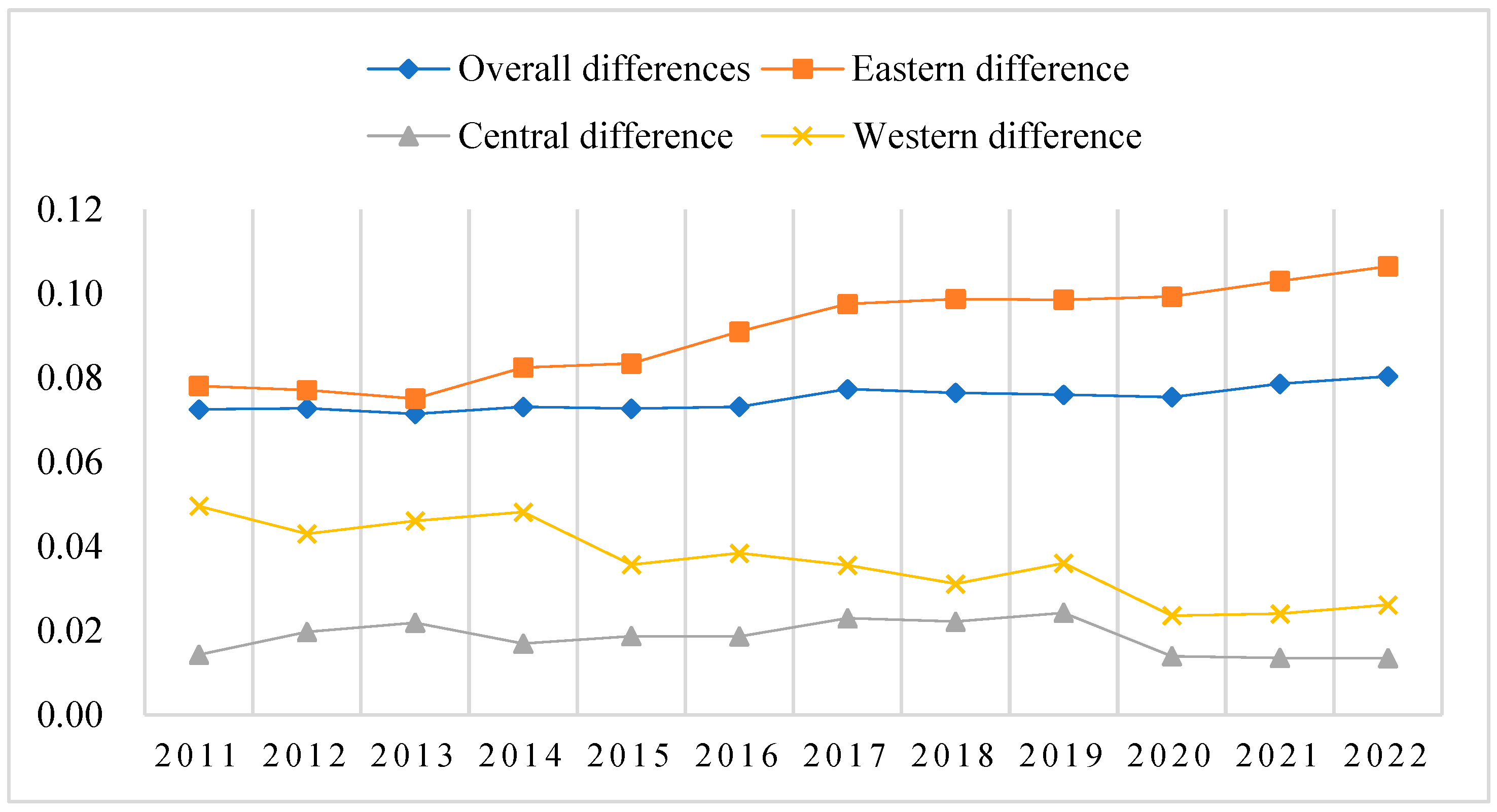
4.4.1. Overall and Intra-Regional Differences
Figure 5 illustrates both the overall and intra-regional disparities in coupling coordination from 2011 to 2022. Nationally, the Gini coefficient fluctuated moderately within the range of 0.0715 to 0.0804, rising from 0.0725 in 2011 to 0.0804 in 2022—suggesting a gradual increase in variation, though the extent remains relatively limited.
Regionally, the average Gini values follow the order eastern > western > central, indicating that internal disparities are most pronounced in the east. Over time, the eastern region’s Gini index shows a consistent upward trend, pointing to widening internal gaps—likely driven by advanced provinces such as Beijing, Shanghai, Guangdong, and Zhejiang outpacing their regional peers. In contrast, the western region exhibits a downward trend in variation, while the central region’s Gini index fluctuates in a cyclical pattern. By 2022, both the central and western regions show reduced Gini values compared to 2011, implying narrowing internal differences in their coordination levels.
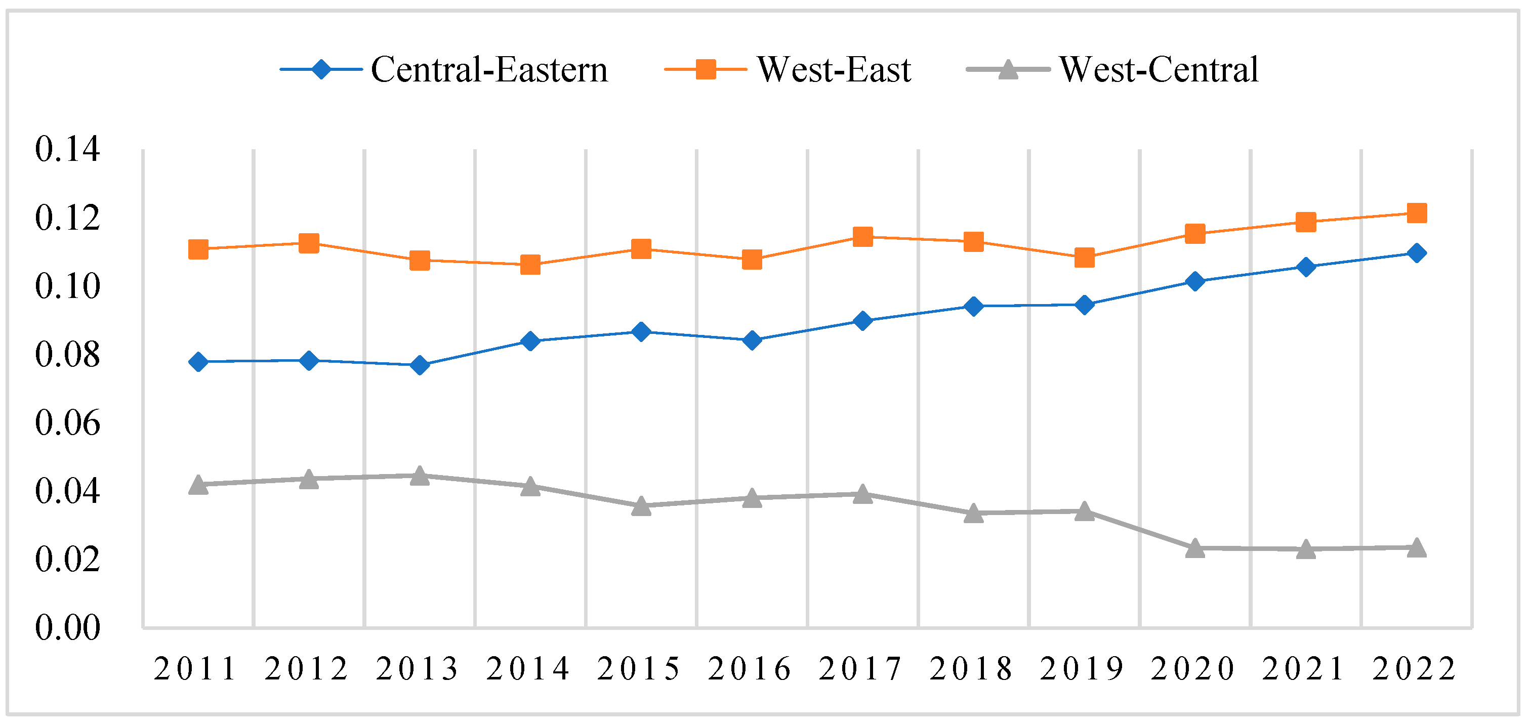
4.4.2. Inter-Regional Differences
Figure 6 illustrates the evolution of inter-regional disparities in coupling coordination from 2011 to 2022. The data reveal a consistent ranking in differences, east–west > east–central > central–west, with the gap between the eastern and western regions being the most significant and that between the central and western regions the smallest. This likely reflects the substantial lead in both financial and economic development enjoyed by eastern provinces over their western counterparts.
Looking at the Gini coefficients, the east–west gap shows a fluctuating upward trend, increasing from 0.1108 in 2011 to 0.1213 in 2022. Similarly, the east–central disparity also rises over time, from 0.0779 to 0.1097. In contrast, the central–west gap exhibits a downward trend, with the Gini coefficient falling from 0.0419 to 0.0235 during the same period. Overall, regional imbalances between the east and other areas are gradually widening—though not drastically—while disparities between the central and western regions are diminishing.
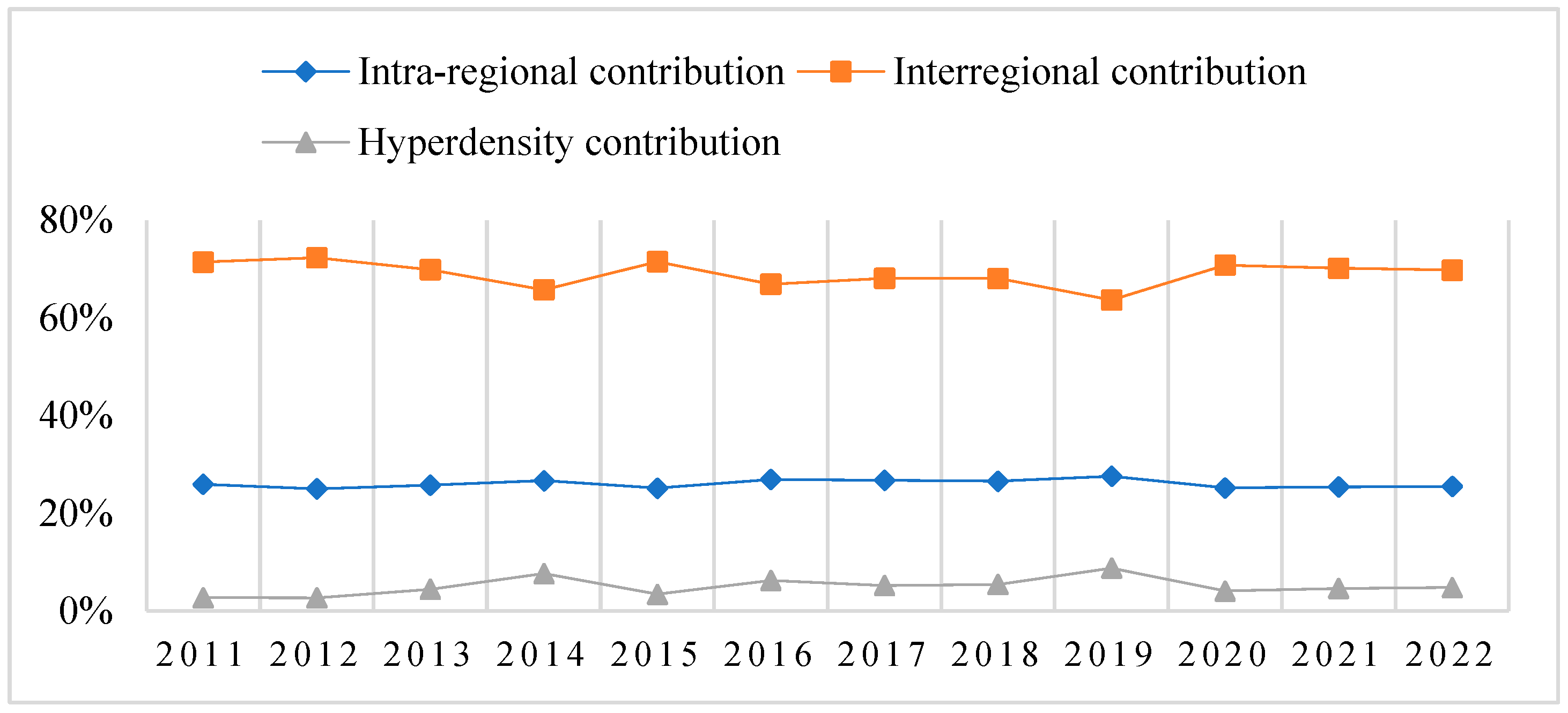
4.4.3. Sources of Differences
Figure 7 shows the sources and contribution rates of regional differences in the coupling coordination degree of the two. It can be seen that the regional differences in the degree of coupling coordination in China mainly come from inter-regional differences, with an average contribution rate as high as 68.891%, followed by intra-regional differences, with an average contribution rate of 26.078%, and the smallest contribution rate of hyperintensity, which is only 5.031%. Overall, inter-regional differences are the main factor behind the differences in the coupled and coordinated development of high-quality financial development and urban–rural economic integration.
4.4.4. Spatial Analysis of the Systematic Coupling of High-Quality Financial Development and Urban–Rural Economic Integration
- (1)
Global spatial autocorrelation: To investigate whether provincial-level coupling coordination exhibits spatial clustering, this study applies the global Moran’s I method. As indicated in
Table 6, the coordination degree between high-quality financial development and urban–rural economic integration remains significantly positive from 2011 to 2022. This suggests the presence of a positive spatial correlation, where the performance in one province is influenced by neighboring regions. The results imply that spatial interdependence plays a role in shaping coordination outcomes. Therefore, fostering regional collaboration—such as interprovincial financial and development partnerships—can help enhance coordinated progress across areas.
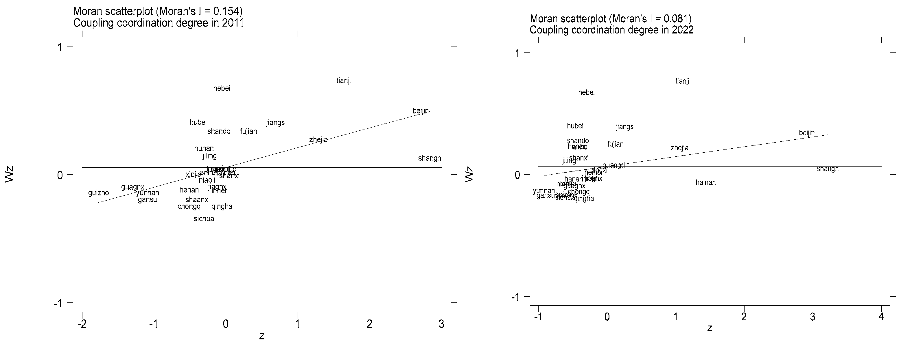
- (2)
Local spatial autocorrelation analysis: To gain deeper insight into the spatial clustering of coupling coordination at the provincial level, this study utilizes local Moran scatter plots for 2011 and 2022. As illustrated in
Figure 8, most provinces display spatial agglomeration patterns concentrated in either high–high or low–low quadrants. Provinces such as Beijing, Tianjin, Shanghai, Zhejiang, Jiangsu, and Fujian, fall into the high–high cluster, indicating that both they and their surrounding areas exhibit strong coupling coordination. Conversely, Shanxi, Inner Mongolia, Guangxi, Yunnan, and Xinjiang, are located in the low–low cluster, suggesting weaker coordination levels in these regions and their neighboring provinces. Mainly constrained by factors such as weak financial foundations, uneven urban and rural development, a single industrial structure, remote geographical location, and lagging financial technology application, it is difficult for financial resources to work effectively and the regional coordinated development capacity is insufficient.
4.5. Analysis of Influencing Factors
Although high-quality financial development and urban–rural economic integration are inherently interlinked and mutually reinforcing, current analysis reveals persistent spatial and temporal disparities in their coordination across regions. These imbalances may stem from several underlying factors, including disparities in human capital, industrial composition, digital infrastructure, governmental policy support, and transportation networks.
Human capital serves as both a catalyst and a beneficiary in this dual development process. A more skilled workforce contributes to agricultural greening, industrial advancement, and seamless urban–rural integration. Individuals with stronger financial literacy and digital competencies also facilitate the broader adoption of innovative financial services, underscoring the critical role of human capital in fostering synergy between finance and integration. Similarly, an upgraded industrial structure enhances the fluidity of production factors, aligns rural industrial development with financial service needs, and improves service quality.
Robust information infrastructure narrows the urban–rural digital divide, fuels e-commerce and digital economy expansion, and strengthens digital finance systems—making it a foundational element of coordinated progress. Additionally, effective government intervention through supportive policies, urbanization initiatives, and institutional reforms creates an enabling environment for both financial modernization and balanced regional development.
4.5.1. Variable Selection and Model Setting
To investigate how human capital, industrial structure, information infrastructure, and government support affect it, this study constructs the following econometric model. Considering that the variables of population size, economic development level, and rural entrepreneurial environment also affect the degree of coupling and coordination of the two (
D) to a certain extent, they are added to the model as control variables, and the explanatory variable is the degree of coupling and coordination (
D). The specific meanings of the variables are shown in
Table 7. The equation is as follows:
where
D is used to denote the degree of coupling and coordination between high-quality financial development and urban–rural economic integration.
X is used to denote the level of human capital, the level of industrial structure, the level of information base, and the level of government support. Control is used to denote control variables,
δi and
τt are used to denote area and time fixed effects, respectively, and
ε is used to denote the random error term.
Based on the availability of data, the above data were selected for this paper, and the raw data were obtained from the China Rural Statistical Yearbook (2011–2022) and the China Statistical Yearbook (2011–2022).
4.5.2. Regression Analysis
- (1)
Base regression analysis
Based on the results of the Hausman test, this paper uses a two-way fixed effects model, and the specific regression results are shown in
Table 8. The results in column (1) show that the regression coefficients of human capital level, industrial structure level, information infrastructure level, and government support level are all significantly positive, indicating that the improvement of population capital level, the optimization of industrial structure, the construction of information infrastructure, and the support of the government can promote the coupled and coordinated development of the two.
Although the two-way fixed-effects model addresses endogeneity from omitted variables, potential reverse causality persists as the current period’s coupling coordination degree (D) may influence key explanatory variables (X)—human capital, industrial structure, information infrastructure, and government support. To mitigate this, all explanatory variables are lagged by one period in the analysis. Employing lagged X within the two-way fixed-effects framework reduces endogeneity concerns, with robustness confirmed by the consistent results in column (2) of
Table 8.
In addition, this paper also shrinks all variables by 1% up and down as well as proposes a regression test for the data of municipalities, and the results from columns (3) and (4) of
Table 8 show that the basic regression results of this paper are still robust.
4.6. Further Analysis: Pollution Reduction and Abatement Effects
The coupling and coordination of the two have obvious pollution reduction effects. Financial development facilitates agricultural transformation by funding green technologies and low-carbon production modes, curbing carbon emissions. Concurrently, urban–rural integration enables the diffusion of advanced urban technologies and eco-friendly management practices into rural areas, enhancing the adoption of environmental protection measures in agriculture. This synergy drives agriculture’s green and low-carbon transition, effectively reducing emissions through improved technological and managerial synergies.
4.6.1. Variable Selection and Model Setting
This paper continues to employ a two-way fixed effects model to empirically examine the emission reduction effect of the coupled and coordinated development between the two. In this model, the explanatory variable is the coupling coordination degree (D); the dependent variable, total agricultural carbon emissions (Tc), is calculated following methodologies from Tang and Chen (2022) [
46] and Fan et al. (2024) [
47]; and control variables include fiscal support for agriculture, infrastructure quality, economic development level, crop disaster severity, and rural electricity consumption, with detailed definitions provided in
Table 9.
Based on the availability of data, the above data were selected for this paper, and the raw data were obtained from the China Rural Statistical Yearbook (2011–2022) and the China Statistical Yearbook (2011–2022).
4.6.2. Regression Analysis
- (1)
Base regression analysis
Based on the results of the Hausman test, this paper uses a two-way fixed effects model for empirical analysis, with the results presented in
Table 10. Column (1) shows that the coupling coordination degree has a significantly negative impact on agricultural carbon emission intensity, underscoring its role in emission reduction. To address endogeneity, lagging explanatory variables by one and two periods ensures that columns (2–3) maintain results consistency. Robustness is further validated through 1% winsorization across variables, reinforcing the reliability of findings.
- (2)
Heterogeneity analysis
Considering regional disparities in development stages and resource allocation, the emission reduction effects of coupling coordination between high-quality financial development and urban–rural integration vary regionally. To assess these differences, China is stratified into eastern, central, and western regions for regression analysis (
Table 11). Results reveal that coupling coordination significantly reduces agricultural carbon emission intensity across all regions, confirming its broad efficacy in curbing emissions. However, regional variation exists; the central region demonstrates the greatest emission reduction impact, while the effect is least pronounced in the eastern region, likely reflecting differing regional priorities and resource distribution.
5. Discussion
This study employs a coupling coordination model to evaluate the synergy between high-quality financial development and urban–rural economic integration. Dynamic evolution trends and regional disparities are assessed through kernel density estimation and Gini coefficient decomposition, while econometric models identify influencing factors and quantify pollution reduction effects of this coordinated development, yielding empirical conclusions.
Firstly, the level of China’s financial high-quality development and urban–rural economic integration and development increased year by year from 2011 to 2022, and the situation of “strong in the east and weak in the west” is obvious. This result is consistent with the results of Chen and Yu (2024) [
48] in measuring the level of urban–rural integration.
Secondly, the level of coordinated development of the two couplings rose steadily from 2011 to 2022, but it is still on the verge of dislocation, with obvious regional differences showing a situation of “high in the east and low in the west”. For example, relying on the advantages of the green finance reform pilot zone, Huzhou has innovated products such as the “Two Mountains Loan” to support ecological agriculture and rural tourism, promote the integration of urban and rural ecological economy, and drive the employment of 32,000 farmers. The integration of urban and rural economies has given rise to the demand for industrial chain finance. For example, the “White Tea Traceability Loan” combined with blockchain lending has a bad debt rate of only 0.8%, realizing a virtuous cycle of financial quality improvement and industrial upgrading.
Thirdly, between 2011 and 2022, there has been a clear polarization phenomenon and ladder effect in the coupling coordination between the two, although this phenomenon has gradually weakened. According to the Gini coefficient analysis, intra-regional differences present the pattern of “east > west > central,” while inter-regional differences show the pattern of “east–west > east–central > central–west.” The differences in the coupled and coordinated development mainly stem from inter-regional disparities, and the coupled and coordinated development of the two exhibits a positive spatial spillover effect.
Fourthly, enhancements in human capital, industrial structure optimization, information infrastructure development, and government support significantly strengthen the coupling and coordination of the two.
Fifthly, the coupled and coordinated development of the two has a significant pollution reduction effect, that is, it effectively reduces agricultural carbon emission intensity.
This paper puts forward the following suggestions:
Firstly, prioritizing the coordinated advancement of high-quality financial development and urban–rural integration is crucial. This entails reforming digital and internet-based inclusive finance to optimize financial resource allocation and align with urban–rural synergy, while bolstering policy-driven financial mechanisms. Targeted investments in rural economic, educational, and ecological sectors, alongside enhancing financial service systems, will foster mutual reinforcement between financial innovation and integrated development.
Secondly, we should focus on regional coordinated development, build a differentiated development framework, and take into account regional differences and spatial spillover effects. In view of the continued existence of the “strong east and weak west” pattern, development policies should be adapted to local conditions. The eastern region should focus on strengthening digital finance and high-end financial services and deepening urban–rural integrated development. The central and western regions should focus on improving financial infrastructure, expanding the coverage of inclusive finance, and strengthening financial support for rural industries and public services.
Thirdly, endogenous motivation and coupling coordination resilience should be enhanced. We should also strengthen vocational education and talent mobility, cultivate compound talents, develop county-level characteristic industries, improve industrial chain finance and green credit support, accelerate the construction of rural 5G networks and digital financial platforms, promote the application of blockchain, artificial intelligence, and other technologies, increase special funding, establish a cross-departmental coordination mechanism, optimize fiscal subsidies and risk prevention mechanisms, and promote the efficient allocation and deep integration of urban and rural resources.
6. Limitation
The limitations of this study are mainly concentrated in several aspects. First, although the coupling and coordinated development of high-quality financial development and urban–rural economic integration is analyzed, due to the constraints of data quality, this paper is based on provincial data, which will ignore more local differences. Secondly, this paper only identified the correlation between high-quality financial development and urban–rural integration, indicating that there is a strong correlation and mutual promotion between the two, but did not further analyze the causal relationship within the two (for example, using a Random Forest model to analyze and rank internal factors). Nevertheless, this paper believes that this will provide a new perspective for both high-quality financial development and the integrated development of urban and rural economies, which will help various regions to promote the coordinated development of the two according to local conditions.


