Abstract
Since China’s reform and opening up over 40 years ago, rapid urbanization has led to significant progress, but also severe air pollution. Understanding how air pollution affects the sustainable development of different city types is crucial for formulating targeted mitigation strategies. Thus, we propose the hypothesis that air pollution affects urban sustainable development through the synergistic interactions of population, industry, space, and society. To test this hypothesis, we construct a simultaneous equation system incorporating pollution, population, industry, spatial, and social factors, utilizing the Three-Stage Least Squares method for estimation. The robustness of our results is rigorously verified. Additionally, to explore deeper mechanisms, we perform a multi-dimensional heterogeneity analysis. Our results indicate that: (1) Air pollution negatively impacts urban sustainable development by reducing urban population size, with a coefficient of −0.950; (2) Air pollution hinders urban sustainable development by reducing manufacturing agglomeration, with a coefficient of −0.962; (3) Air pollution induces disordered urban spatial expansion, undermining sustainable development, with a coefficient of 2.596; and (4) Air pollution leads to stricter environmental rules, with a coefficient of 17.428, and these rules boost urban sustainability in the long term. Heterogeneity analysis further reveals that the intensity, direction, and statistical significance of air pollution’s effects vary across cities with different regional characteristics, pollution levels, population scales, industrial structures, spatial patterns, and regulatory intensities.
1. Introduction
Since the implementation of reform and opening-up policies, China’s urban development has made remarkable progress over the past four decades. Data from the National Bureau of Statistics show that China’s urbanization rate increased from less than 20% at the beginning of the reform period to 67% by the end of 2024 [1]. Concurrently, urban built-up areas expanded significantly from 47,900 square kilometers to 64,500 square kilometers between 2013 and 2023 [2]. However, despite these achievements, persistent challenges related to air pollution remain. Numerous cities in China continue to report PM2.5 concentrations that exceed World Health Organization standards [3], with severe smog events still occurring during unfavorable meteorological conditions in autumn and winter, posing serious risks to public health and urban livability [4].
Air pollution profoundly hinders urban sustainable development through synergistic interactions across population, industry, space, and society: it drives skilled labor outmigration from polluted cities while attracting vulnerable groups lacking relocation options, disrupting labor markets and straining social services; polluting industries often cluster in regions with loose regulations, creating a vicious cycle where economic activities degrade air quality, depress land values, and deter high-tech investment, worsening regional disparities; and its disproportionate health impacts on marginalized communities deepen socioeconomic inequalities by increasing productivity losses and healthcare burdens [5,6]. Recognizing these interconnected mechanisms is crucial for policymakers to design targeted interventions to balance ecological protection and inclusive economic growth, advancing long-term sustainability amid regional disparities.
Current research has predominantly centered on the mechanisms through which urban development gives rise to air pollution [7]. This focus has often overshadowed the exploration of the reverse causal link—how air pollution influences the trajectories of urban development. Such a one-sided perspective limits our understanding of the complex feedback loops between urbanization and environmental quality. Furthermore, the majority of existing studies tend to analyze the isolated impacts of air pollution on specific domains, such as public health or ecological systems [8]. This fragmented approach fails to capture the interconnectedness of these issues within the broader framework of urban sustainable development. By treating these impacts in isolation, researchers and policymakers may overlook synergistic effects and miss opportunities to design holistic solutions that address population, economic, and social dimensions simultaneously. This study aims to fill these gaps by comprehensively analyzing the multi-dimensional effects of air pollution on China’s urban sustainability, with a particular focus on inter-city heterogeneity. The findings will enhance our theoretical understanding of the dynamics between pollution and development, offering valuable policy insights for other rapidly urbanizing countries. Amid the global trend of urban expansion, this research provides evidence-based recommendations for promoting healthier and more sustainable urban development paths.
2. Literature Review and Research Hypotheses
2.1. Literature Review
Historically, research has largely focused on the mechanisms by which urban development influences air pollution. Many studies use urban development indicators—such as urban sprawl, industrial restructuring, population dynamics, and transportation infrastructure expansion—as independent variables, while air pollution indicators (e.g., pollutant concentration variations and pollution event frequency) are treated as dependent variables [9]. These studies aim to clarify the relationships between urban development processes and air pollution, ultimately informing policy interventions for pollution mitigation through urban planning.
However, a critical gap in the literature is the lack of comprehensive studies examining reverse causality, (i.e., how air pollution impacts urban development and the underlying mechanisms). While some scholars have explored bidirectional relationships, such as Liang et al., who identified the inhibitory effects of haze pollution on urban development through spatial simultaneous equations [10], these analyses lacked a deeper mechanistic understanding. Notably, few studies explicitly frame air pollution as an independent variable affecting urban development. Nevertheless, indirect evidence suggests this relationship exists, with studies exploring how pollution impacts urban subsystems, such as population mobility, economic performance, governance capacity, and resident well-being.
These subsystems, particularly population dynamics, offer insights into the redistributive effects of pollution. Studies on air pollution-driven population redistribution present varied findings. Zhang et al. observed pollution-driven outmigration primarily in economically developed regions, such as the Yangtze River Delta and Chengdu-Chongqing urban clusters [11], whereas Xi and Liang found delayed interregional migration effects due to environmental factors [12]. Sun and Sun demonstrated that haze pollution negatively correlates with long-term urban settlement intentions among migrants, particularly among older populations and interprovincial migrants [13]. Despite these advances, several critical questions remain unexplored: whether pollution drives counter-urbanization or alters urban agglomeration patterns through secondary rural-urban population shifts.
Beyond population shifts, the economic repercussions of pollution further shape urban trajectories. Research has highlighted the economic costs of pollution through its impact on health and labor supply [14]. Chen et al. estimated that the coal heating policy in northern China reduced life expectancy by 5.5 years due to exposure to particulate matter [15]. National assessments indicate that air pollution costs rose to 305.1–1001.2 billion yuan from 2006 to 2014, with health-related productivity losses making up 73% of the total, as reported by the Ministry of Environmental Protection in 2014. Micro-level analyses have shown that pollution reduces the labor supply of migrant workers by 0.011–0.019 days per 1% increase in pollution [16]. Regional CGE modeling predicts significant GDP losses (2.15–2.79%) in the Beijing-Tianjin-Hebei region by 2020 [17]. However, no studies have explored how pollution affects industrial spatial restructuring, structural upgrading, or income distribution—critical aspects of urban economic transformation.
The intersection of pollution and social systems reveals further complexities. Research on urban social development examines both governance responses and well-being impacts. Local governments exhibit nonlinear patterns in environmental expenditure: pollution increases lead to reduced spending at lower pollution levels, with no proportional increase at higher levels [18]. Fiscal behavior also mediates economic-environmental tradeoffs [19]. Resident well-being studies show that subjective pollution perceptions significantly affect happiness [20], with eastern populations showing greater sensitivity [21]. Moreover, corporate ESG (Environmental, Social, and Governance) behavior, an important aspect of the social dimension impacted by air pollution, has drawn increasing attention. Lu et al. highlighted the connection between environmental policies, pollution control, and corporate ESG investment [22]. Song et al. suggested that a latecomer advantage exists for enhancing ESG performance under regulatory pressure in China’s digital economy [23]. Torres et al. emphasized the social benefits of corporate ESG initiatives [24]. However, existing studies on the above-mentioned purposes rarely take into account the heterogeneity issues, such as regional differences or industry disparities, which may lead to limitations in the universality and accuracy of the research conclusions.
This review identifies three key limitations: (1) A fragmented approach to examining urban subsystems without an integrative framework; (2) Insufficient focus on pollution’s systemic effects on urban sustainability; and (3) Limited heterogeneity analysis. Building on these gaps, our study first proposes research hypotheses based on existing literature and the definition of urban sustainable development, positing that air pollution affects urban sustainability through four dimensions: population, industry, space, and society. Subsequently, an empirical model is constructed and estimated using the Three-Stage Least Squares (3SLS) method. Following the acquisition of baseline regression results, robustness tests are conducted to verify the findings. Additionally, multiple heterogeneity tests are performed on the results. Through this approach, our study contributes by: (1) pioneering a systematic investigation of air pollution’s feedback effects on urban development; (2) conceptualizing “urban sustainable effects” from a multidimensional perspective; and (3) clarifying the spatial and structural heterogeneities in the pollution-development relationship. These findings will provide key insights for formulating sustainable urbanization strategies under environmental constraints.
2.2. Research Hypotheses
2.2.1. The Concept of Urban Sustainable Development
The modern conceptualization of sustainable development was first formally articulated in Our Common Future (1987) by the World Commission on Environment and Development. This influential report marked a shift from viewing environmental protection and development as opposing goals to reconciling them through an integrated global ethic that includes economic progress, social equity, and environmental stewardship. Subsequent scholarly discussions have refined this concept into three interconnected pillars: economic sustainability, ecological sustainability, and social sustainability [25]. A key institutional milestone occurred at the 1992 United Nations Conference on Environment and Development, where the Rio Declaration and Agenda 21 were adopted. These documents outlined actionable guidelines for sustainable development across social, economic, and environmental spheres. They emphasized inclusive social development, poverty alleviation through international cooperation, and ecosystem conservation via responsible resource management. While interpretations of sustainable development have evolved, there is consensus that true sustainability must address economic viability, social equity, and ecological integrity simultaneously.
As primary centers of human activity, cities represent both the epicenter of human-environment conflicts and the frontline for implementing sustainability strategies. The formal concept of urban sustainability emerged through the UN’s Sustainable Cities Program in the 1990s, which spurred theoretical advancements by integrating multiple disciplines. Economists applied environmental valuation models and green consumption theories, sociologists used surveys and network analysis to study livable cities and environmental behavior, and ecologists introduced footprint analysis and habitat indices to assess urban carrying capacity. These efforts led to the development of concepts like resilient cities and low-carbon urbanism [26]. In contemporary urbanization contexts, traditional ecological perspectives are insufficient to capture the complexity of urban sustainability. Modern interpretations view it as a dynamic, human-centered system where population mobility, industrial agglomeration, spatial sprawl, and social regulation interact synergistically. This evolution reflects both the multidimensional nature of urban challenges and the need for holistic, evidence-based policy approaches that transcend single-dimensional solutions.
2.2.2. Research Hypotheses on the Impact of Air Pollution on Urban Sustainable Development
Urban development, which is marked by high population densities, intense industrial production, uncontrolled spatial expansion, and traffic congestion, exacerbates the exposure of residents to air pollution [9]. Unlike rural areas, urban environments face greater challenges in dispersing pollutants, and the elasticity of pollutant emissions increases as urban populations grow [27]. Moreover, air pollution is closely linked to respiratory diseases, higher mortality rates, and increased healthcare visits [28], particularly in northern China’s cities, where coal-burning heating systems contribute to higher pollution levels [14], thus reducing residents’ working lifespans. High-skilled, high-income individuals, who prioritize quality of life, often relocate to cities with better air quality. This outmigration diminishes the urban human capital essential for driving innovation, economic consumption, and long-term growth. As a result, the loss of such talent hampers urban innovation, reduces market dynamism, and impedes sustainable economic development. Thus, we propose:
Hypothesis 1:
Air pollution negatively impacts urban sustainable development by reducing urban population size.
Air pollution significantly disrupts manufacturing processes. Pollutants such as gases and particulate matter accelerate the corrosion of equipment, particularly in industries such as chemicals and steel, where high emissions degrade production machinery [29]. This increases maintenance costs, disrupts production, and reduces overall efficiency. Furthermore, growing environmental awareness has shifted consumer demand toward green products [30]. Companies in heavily polluted areas face declining demand and diminished competitiveness, motivating them to relocate to cleaner regions. This relocation reduces industrial agglomeration, weakening inter-firm synergies, knowledge spillovers, and economies of scale. Consequently, such fragmentation inhibits technological diffusion, supply chain optimization, and overall economic resilience. Hence, we hypothesize:
Hypothesis 2:
Air pollution hinders urban sustainable development by reducing manufacturing agglomeration.
To reduce the health impacts of air pollution, governments often relocate polluting industries to the outskirts of cities. This displacement affects supporting services (such as logistics and housing) and employees, thereby accelerating urban sprawl [31]. Simultaneously, residents seeking cleaner environments migrate to suburban areas, which further intensifies unplanned expansion, as seen in the growing real estate demand in Beijing’s satellite cities [32]. This sprawl leads to inefficient land use, encroaches upon farmland and ecosystems, raises infrastructure costs, and depletes biodiversity, thus creating long-term sustainability challenges. Therefore, we posit:
Hypothesis 3:
Air pollution induces disordered urban spatial expansion, undermining sustainable development.
Governments recognize the significant threats air pollution poses to urban ecosystems, public health, and city reputations, sparking widespread societal concern. In response, policymakers strengthen environmental regulations to improve air quality and encourage sustainable urban development [33]. These regulatory measures often include implementing stricter emission standards, reducing pollutant concentration limits, imposing more rigorous total emission controls for industrial pollutants, improving monitoring and enforcement mechanisms, and providing fiscal incentives such as tax breaks and R&D subsidies to promote green innovation. While these regulations may initially increase production costs due to the need for investments in pollution control and compliance measures, their long-term benefits outweigh these short-term economic drawbacks. By forcing industries to abandon outdated production methods and shift toward cleaner, more technology-intensive operations, these regulations foster industrial upgrading. Additionally, they stimulate growth in the environmental protection sector, creating new economic opportunities and aligning economic development with ecological preservation [34]. This dual effect ultimately contributes to more sustainable urban development pathways. Consequently, we propose:
Hypothesis 4:
Air pollution prompts governments to strengthen environmental regulations, which, despite short-term adjustment costs, contribute to sustainable urban development in the long term.
The comprehensive research framework exploring the impact of air pollution on urban sustainability across population, industrial, spatial, and social dimensions is illustrated in Figure 1.
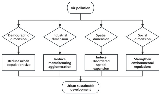
Figure 1.
Research Framework.
3. Methods, Data, and Model Validation
3.1. Model Design
To comprehensively assess the impact of air pollution on urban sustainable development, this study endeavors to dissect its effects across four pivotal dimensions: urban population, industry, spatial structure, and social development. These dimensions are intricately intertwined, forming a complex web of interdependencies. For instance, changes in the urban population can significantly influence the demand for industrial products and services, thereby impacting the industrial structure and development. Conversely, industrial development can attract or repel population, altering the demographic composition of the city. Considering these multifaceted and reciprocal influences, accurately accounting for potential cross-dimensional effects becomes indispensable when analyzing the specific impacts of air pollution. This is precisely why the following general form of the air pollution impact equation is constructed:
where for sample region i at time t pollutionit, PSit, Aggit, Sprawit, and Envirit denote air pollution and the four sustainable development dimensions (population, industry, space, and society); Zit represents control variables affecting urban sustainable development; ηit is the error term; β1,2,3,4, β′1,2,3,4, β″1,2,3,4, β‴1,2,3,4 capture the endogenous relationships among sustainable development dimensions.
3.2. Parameter Estimation Methods
The estimation methods for simultaneous equations can be classified into two main categories: single-equation estimation methods (also called “limited information methods”) and system estimation methods (known as “full information methods”). The primary difference between these approaches lies in how estimation is performed—the single-equation method estimates each equation separately, while the system estimation method estimates all equations jointly as part of an integrated system. Among these methods, two-stage least squares (2SLS) is the most commonly used single-equation method, while three-stage least squares (3SLS) is the most commonly applied system estimation technique.
When a structural equation satisfies the identification condition, where the number of excluded exogenous variables equals or exceeds the number of included endogenous explanatory variables, and all excluded exogenous variables are valid instrumental variables, the instrumental variable method can be applied. Under the classical assumptions of homoskedasticity and no autocorrelation in the disturbance term, 2SLS emerges as the most efficient instrumental variable estimator, which explains its widespread use as the standard single-equation approach. The instrumental variable framework allows for linear combinations of instruments, maintaining their validity by preserving essential properties of correlation and exogeneity. The 2SLS method specifically generates the most asymptotically efficient linear combination of instruments under spherical disturbance assumptions. The process involves two stages: initially performing OLS regressions of each explanatory variable on all instrumental variables to obtain fitted values representing the exogenous components, followed by regression of the original dependent variable on these fitted values, which are then used as instruments.
However, greater efficiency can be achieved using system estimation methods, which account for inter-equation relationships, including correlations among disturbance terms that single-equation methods disregard. While the 3SLS method is susceptible to specification errors in individual equations, which can affect the entire system, it offers efficiency gains by combining 2SLS with seemingly unrelated regression (SUR) techniques. In systems with multiple equations, OLS estimation remains consistent but inefficient when equations contain no endogenous variables, as it fails to exploit potential error correlations across equations—this limitation is addressed by SUR. When endogenous variables are present, 2SLS provides consistent estimates for individual equations but ignores cross-equation error correlations, making system-wide 3SLS estimation the more efficient alternative. The 3SLS procedure mirrors 2SLS in its first two stages but then estimates the system’s disturbance covariance matrix and applies generalized least squares (GLS) estimation, like the SUR method.
This study confronts the endogeneity issue arising from bidirectional causality between the dependent variable (air pollution levels) and key explanatory variables (sustainable development indicators). The relationship runs in both directions: urban development patterns may either worsen environmental degradation through extensive expansion or mitigate pollution through sustainable practices, while, simultaneously, pollution levels may influence urban development by affecting demographic distribution, economic behaviors, and policy responses. This reciprocal relationship makes OLS estimates biased and inconsistent. Although 2SLS can address the endogeneity concern, its single-equation framework fails to capture potential error correlations across equations. The 3SLS approach effectively resolves both issues, making it the preferred estimation method for this analysis.
3.3. Indicator Selection and Preprocessing
This study uses PM2.5 concentration as the primary measure of urban air pollution, a key indicator closely associated with the recurring haze episodes observed in China in recent years. These frequent haze events in specific regions have posed significant risks to public health and quality of life, with PM2.5 (fine particulate matter measuring 2.5 microns or smaller) serving as a major component. Due to their minute size, PM2.5 particles remain suspended in the atmosphere for extended periods and can travel over long distances. In addition to degrading air quality, these particles also absorb toxic substances, including carcinogens such as polycyclic aromatic hydrocarbons, which makes their concentration an effective proxy for assessing urban air pollution levels.
To assess urban sustainable development, this study adopts a multidimensional framework based on the theoretical concepts outlined in Section 2. The framework incorporates indicators that span the population, industry, spatial, and social dimensions. Urban population size (PS) represents demographic changes, manufacturing agglomeration (Agg) reflects industrial development, urban spatial sprawl (Spraw) quantifies expansion patterns, and environmental regulation intensity (Envir) captures the extent of social governance efforts.
The simultaneous equation system model requires distinct variables for each equation while accommodating shared influences. To control for potential impacts on population, industry, spatial, and social development, three common control variables are included across all equations: per capita green space (PGreen), per capita road area (Road), and traffic congestion level (TC). Unique identifying variables are assigned to each equation: per capita GDP (PGDP) for the population equation, transportation accessibility (FV) for industry, population density (PD) for spatial expansion, and energy consumption intensity (SE) for the social governance equation.
In summary, PM2.5 concentration is used as the measure for urban air pollution, while PS, Agg, Spraw, and Envir represent the four pillars of sustainable development. The simultaneous equation system incorporates PGreen, Road, and TC as universal controls, with PGDP, FV, PD, and SE as equation-specific identifiers. The detailed definitions, interpretations, and units of these variables are provided in Table 1.

Table 1.
Variable Description.
Due to data availability constraints and the exclusion of prefecture-level cities with significant missing data, the selected indicators in this study exhibit variations in time coverage and sample size. The PM2.5 concentration data, which spans 272 China’s prefecture-level and above cities from 2004 to 2016, were sourced from the Atmospheric Composition Analysis Group at Dalhousie University in Canada. Data for PS, Agg, Spraw, PGreen, Road, TC, PGDP, FV, PD, and SE were collected from 275 cities in China, primarily derived from the China Urban Statistical Yearbook and the China Urban and Rural Construction Statistical Yearbook. Some of these data required additional processing and recalculation for this study. The Envir data were manually collected by the authors and underwent multiple processing steps, ultimately covering the same period from 2004 to 2016. Table 2 presents detailed descriptive statistics and complete data sources for all variables.
Table 2.
Variable Statistical Description.
3.4. Model Validity Test
Endogeneity can result in biased or inconsistent estimations. This study identifies two potential sources of endogeneity: (1) Omitted variable bias, where the model may neglect important determinants of air pollution; and (2) Reverse causality, as urban development and air pollution are likely interconnected in a bidirectional relationship. In the absence of ideal instrumental variables (IVs), we utilize the 3SLS method to mitigate endogeneity. This method is particularly effective in addressing simultaneous equations using instrumental variable techniques. Specifically, diagnostic tests for weak instruments and over-identification are conducted within the IV regressions involving PM2.5, population size, manufacturing agglomeration, and spatial spillovers.
The test results, as shown in Table 3, confirm that all instrumental variables satisfy the relevance (i.e., no weak instruments) and exogeneity (i.e., no over-identification) conditions. Additionally, the first-stage estimates demonstrate the strong predictive power of the exogenous variables for the endogenous regressors, collectively validating the robustness of our 3SLS estimates.
Table 3.
Instrumental Variable Test.
To facilitate a better understanding of the research methods in this article, we have meticulously designed and drawn a clear flowchart, as depicted in Figure 2.
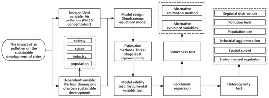
Figure 2.
Research Methods.
4. The Impact of Air Pollution on Urban Sustainable Development
4.1. Benchmark Regression and Discussion
The Hausman test is initially conducted, indicating that the panel fixed-effects model is more appropriate for this sample. Further testing reveals the absence of significant time effects, suggesting that only individual fixed effects need to be considered for estimation. However, since the panel fixed-effects model is limited to single-equation estimation and cannot address the inherent endogeneity issue, we adopt a simultaneous equations model to examine the mechanism through which air pollution influences urban sustainable development. Given that the simultaneous equations model is typically designed for cross-sectional data, we remove individual effects at the time level to facilitate estimation for panel data. The acceptance of the “no time effect” null hypothesis validates this approach. Unless otherwise stated, all subsequent model estimations are based on data adjusted for individual effects.
Table 4 presents the results of the 3SLS estimation for the impact of air pollution (PM2.5) on urban sustainable development. Columns (1) to (4) report the population scale, industrial agglomeration, spatial expansion, and environmental regulation equations, respectively. The results demonstrate that PM2.5 significantly reduces urban population size and manufacturing agglomeration, while exacerbating urban spatial expansion. Additionally, as PM2.5 concentrations rise, the intensity of environmental regulation increases, aligning with theoretical expectations.
Table 4.
Basic Estimation Results of the Impact of Air Pollution on Urban Sustainable Development.
PM2.5 significantly impacts urban sustainable development across various aspects. In the Population Scale Equation, PM2.5 has a notably negative effect on urban population size (coefficient = −0.950, significant at the 1% level), as increased public awareness of health risks encourages population outflow, particularly in smaller and medium-sized cities heavily affected by pollution This trend indicates that population mobility is becoming more sensitive to changes in air quality (Hypothesis 1). In the Industrial Agglomeration Equation, PM2.5 negatively affects industrial agglomeration (coefficient = −0.962, significant at the 1% level) due to two factors: population loss, which indirectly reduces manufacturing employment, and stricter environmental regulations that prompt high-pollution industries to relocate or upgrade, thereby reducing agglomeration (Hypothesis 2). The Spatial Expansion Equation shows that PM2.5 accelerates urban spatial expansion (coefficient = 2.596, significant at the 1% level), with rising pollution levels pushing polluting industries to suburban areas and encouraging residents to migrate to less polluted regions, further promoting spatial dispersion (Hypothesis 3). Finally, in the Environmental Regulation Equation, PM2.5 significantly increases the intensity of environmental regulations (coefficient = 17.428, significant at the 1% level), as both central and local governments face mounting public pressure to implement stricter pollution control measures due to the severe health risks associated with air pollution (Hypothesis 4).
4.2. Robustness Test
4.2.1. Alternative Estimation Method
In the baseline analysis, the 3SLS method is employed to estimate the simultaneous equations model. To further assess the robustness of the findings, we re-estimate the model using the 2SLS approach.
The results from the 2SLS estimation (Table 5) largely align with those from the 3SLS approach for most variables. However, the negative effect of PM2.5 on industrial agglomeration loses statistical significance. This discrepancy may arise because 2SLS does not account for potential correlations across the disturbance terms of simultaneous equations, which could influence coefficient significance. Nevertheless, the overall consistency of the results across the two methods reinforces the robustness of our key findings.
Table 5.
Robustness Test: 2SLS Estimation Results.
The 3SLS method is typically applicable only to ordinary simultaneous equations models. In this study, we employ the Spatial Durbin Model (SDM) to estimate equations for pollution, population, industry, space, and society. The estimation results reveal statistically significant spatial spillover effects across all variables. To further examine the spatial effects of these core variables in the simultaneous equations framework, we adopt the Generalized Spatial Three-Stage Least Squares (GS3SLS) method to estimate the interactive relationship between urban development and air pollution. However, it should be noted that the GS3SLS method can only simultaneously estimate two equations at most. Consequently, this study sequentially integrates the four dimensions of urban development (population, industry, space, and society) with the air pollution equation for regression. While this approach partially neglects the systematic influences of the other three equations, it maximizes the incorporation of systemic urban development effects into the model. Therefore, the estimation results can still provide a “partial-yet-representative” perspective on the overall system.
Table 6 presents the estimation results of the spatial simultaneous equations model for urban development and air pollution. Specifically, Models 1, 2, 3, and 4 correspond to the joint estimation outcomes of the air pollution equation with the urban development equations (population, industry, space, and society), respectively.
Table 6.
Robustness Test: GS3SLS Estimation Results.
As evidenced by Model 1, neither the spillover effects of PM2.5 nor population size demonstrates statistically significant impacts on other cities’ population scales. Model 2 reveals that both urban PM2.5 and industrial agglomeration exert significantly negative spillover effects on neighboring cities’ industrial agglomeration. This phenomenon may be attributed to the “siphon effect,” whereby cities with higher agglomeration levels attract manufacturing labor from less agglomerated areas. Furthermore, when a city’s industrial agglomeration intensifies, it reduces its own PM2.5 emissions while inadvertently increasing ambient pollution in surrounding areas, manifesting a “pollution depression” characteristic within the region. This mechanism partially explains the negative spillover effect of PM2.5 observed in Model 2. Although skilled labor migrates toward superior opportunities, air pollutants disperse indiscriminately. When neighboring cities’ PM2.5 spills over, it naturally triggers outmigration of manufacturing populations, thereby diminishing local industrial agglomeration. Model 3 indicates that urban PM2.5 and spatial expansion significantly positively affect adjacent cities. This dual effect occurs because: (1) Local PM2.5 spillovers exacerbate regional pollution levels; and (2) an “imitation effect” emerges wherein real estate developers and homebuyers in neighboring cities replicate pollution-avoidance strategies (e.g., constructing residential complexes in better-ventilated suburban areas), consequently accelerating urban sprawl. Model 4 demonstrates that spillover effects from both PM2.5 and environmental regulations significantly enhance neighboring cities’ regulatory stringency. When a city strengthens its environmental regulations, surrounding jurisdictions respond competitively by intensifying their own regulatory frameworks to demonstrate proactive pollution governance. This pattern confirms the consistency and synchrony in regional environmental policy adjustments, where cities systematically incorporate PM2.5 spillover effects as key indicators for regulatory calibration. In summary, the empirical results remain robust after accounting for spatial spillover effects across all variables.
4.2.2. Alternative Explained Variables
To further substantiate the robustness of our results, we conduct additional tests by substituting the urban sustainable development variables with alternative measures. The population size variable is replaced with the population growth rate (Popgrow), calculated as the natural growth rate between 2004 and 2016, with data sourced from the China Urban Statistical Yearbook. Larger cities typically exhibit higher population growth rates, making this alternative measure a valid proxy for population dynamics. To capture manufacturing agglomeration, we replace location entropy with nighttime light intensity (Light). This variable reflects economic activity and industrial concentration during the 2004–2016 period, based on data from NOAA. This measure better reflects urban industrial concentration and addresses potential limitations of location entropy. We measure spatial spread using the urban built-up area ratio (PCA), with data spanning 2004–2016 from the China Urban and Rural Construction Statistical Yearbook. Since urban expansion is inherently linked to the growth of built-up areas, this ratio provides a direct and intuitive measure of spatial development. Following Zhu et al., we substitute the proportion of environmental word frequency with a composite index for pollutant removal rate (ER) [35]. This index incorporates five indicators: SO2 removal rate, soot removal rate, industrial solid waste utilization rate, domestic sewage treatment rate, and municipal waste harmless treatment rate, all weighted using the entropy method. The inverse of the composite score serves as a proxy for regional environmental regulation intensity.
Table 7 presents the re-estimated results. Despite some minor variations in the magnitude and significance of coefficients, the overall directional effects remain consistent across all key variables, further supporting the reliability and robustness of our initial findings.
Table 7.
Robustness Test: Alternative Variable Specifications.
4.3. Heterogeneity Test
To comprehensively explore the impact of PM2.5 on urban sustainable development, we further conducted a heterogeneity analysis to investigate the effects under varying conditions, including different regions, pollution levels, population sizes, industrial agglomeration degrees, spatial expansion extents, and environmental regulation intensities. The specific results are presented in Table 8. Below is a more in-depth analysis focusing on these different dimensions of heterogeneity.
Table 8.
Heterogeneity across different dimensions.
4.3.1. Heterogeneity of Regional Distribution
Given the vast geographical diversity and uneven regional development within China, there are substantial disparities in urbanization levels and natural conditions across the eastern, central, western, northeastern, southern, and northern regions. These regional variations may result in different effects of air pollution on urban sustainable development. To explore this potential heterogeneity, we divide our sample into six regional subsamples. Table 8(a) presents the regional heterogeneity test results regarding the impact of air pollution on urban sustainable development.
In the Population Equation, significant negative impacts of PM2.5 are observed in Eastern China (coefficient = −0.451, significant at the 1% level), Western China (coefficient = −0.262, significant at the 1% level), and Southern China (coefficient = −0.802, significant at the 1% level), indicating that higher pollution drives population decline in these regions. This likely reflects migration away from polluted coastal manufacturing hubs (East/South) and ecologically fragile areas (West). Conversely, Northern China shows a positive association (coefficient = 0.691, significant at the 10% level), potentially due to industrial path dependence or energy-intensive economic structures limiting outmigration. Northeast China exhibits a weaker negative effect (coefficient = −0.102, significant at the 10% level), while Central China shows no statistical significance.
In the Manufacturing Agglomeration Equation, significant negative effects emerge in Central China (coefficient = −0.836, significant at the 1% level), Southern China (coefficient = −1.170, significant at the 1% level), Northern China (coefficient = −0.763, significant at the 1% level), and Northeast China (coefficient = −0.479, significant at 5% level). This suggests PM2.5 inhibits industrial clustering, particularly in heavy manufacturing and export-oriented regions (North/Central/South) where environmental compliance costs may accelerate relocation. Eastern and Western China show statistically insignificant coefficients, implying weaker pollution constraints on agglomeration—possibly due to advanced abatement technology in the East or resource-based industrialization in the West.
In the Spatial Spread Equation, PM2.5 significantly reduces sprawl in Eastern China (coefficient = −2.771, significant at the 1% level) and Western China (coefficient = −2.404, significant at the 1% level), likely reflecting land-use regulations in densely populated eastern metros and ecological conservation policies in western regions. Conversely, it accelerates sprawl in Central China (coefficient = 3.319, significant at the 1% level) and Southern China (coefficient = 3.723, significant at the 1% level), indicating pollution-driven decentralization of industries and populations toward peri-urban areas. Northern China shows moderate sprawl promotion (coefficient = 1.111, significant at the 10% level), while Northeast China is insignificant.
In the Environmental Regulation Equation, PM2.5 exhibits universally positive and highly significant effects across all regions: Eastern China (coefficient = 12.117, significant at the 1% level), Central China (coefficient = 18.862, significant at the 1% level), Western China (coefficient = 14.700, significant at the 1% level), Northeast China (coefficient = 2.466, significant at the 1% level), Southern China (coefficient = 24.004, significant at the 1% level), and Northern China (coefficient = 18.834, significant at the 1% level). This robust pattern confirms that worsening air pollution consistently strengthens environmental regulatory responses nationwide. The intensity varies regionally, with Southern and Central China showing the strongest feedback—likely due to higher population exposure and economic capacity for policy intervention.
4.3.2. Heterogeneity of Pollution Concentration Level
To examine the influence of varying levels of air pollution on urban sustainable development, we classify cities into three categories based on the WHO’s (2005) PM2.5 guidelines: high pollution (PM2.5 > 35 μg m−3), medium pollution (15 μg m−3 < PM2.5 ≤ 35 μg m−3), and low pollution (PM2.5 ≤ 15 μg m−3). The results, presented in Table 8(b), reveal distinct patterns across pollution levels.
In the Population Equation, significant heterogeneity exists across pollution levels. In high-pollution areas, PM2.5 exerts a strong negative influence on population (coefficient = −2.180, significant at the 1% level), indicating that severe air pollution drives population outflow. The effect remains negative but substantially weaker in medium-pollution regions (coefficient = −0.306, significant at the 1% level). Conversely, in low-pollution areas, PM2.5 shows a paradoxical positive association (coefficient = 0.430, significant at the 1% level), suggesting that cleaner environments may attract population growth despite baseline pollution exposure. This reversal implies a threshold effect where pollution’s deterrent impact dominates only beyond moderate concentrations.
In the Manufacturing Agglomeration Equation, heterogeneity is pronounced. High pollution significantly suppresses industrial clustering (coefficient = −1.666, significant at the 1% level), consistent with firms avoiding locations with extreme pollution costs. The effect becomes statistically insignificant in medium-pollution zones (coefficient = −0.057, not significant), indicating a neutral impact. Notably, low-pollution areas exhibit a positive relationship (coefficient = 1.150, significant at the 10% level), implying that cleaner environments may foster industrial agglomeration, possibly due to enhanced productivity or regulatory flexibility absent in heavily polluted regions.
In the Spatial Spread Equation, PM2.5’s impact reverses direction across pollution strata. High pollution strongly accelerates spatial expansion (coefficient = 5.652, significant at the 1% level), likely reflecting urban dispersal driven by pollution avoidance or land-intensive industrial relocation. Conversely, medium pollution correlates with reduced sprawl (coefficient = −1.375, significant at the 5% level), potentially indicating denser development under manageable pollution levels. In low-pollution areas, sprawl increases again (coefficient = 2.256, significant at the 5% level), possibly due to economic growth enabling suburbanization in cleaner environments.
In the Environmental Regulation Equation, PM2.5 consistently heightens regulatory responses across all strata but with varying intensity. The effect is strongest in high-pollution areas (coefficient = 26.627, significant at the 1% level), reflecting urgent policy interventions under severe pollution. Medium-pollution regions show a substantial but reduced effect (coefficient = 16.390, significant at the 1% level), while low-pollution zones still exhibit a robust positive association (coefficient = 21.969, significant at the 1% level). This gradient (high > low > medium) suggests that regulatory pressure is most intense under extreme pollution but remains elevated in cleaner areas, possibly due to proactive policies or heightened public awareness.
4.3.3. Heterogeneity of Population Size
Population samples are divided based on city size, according to national classifications for large, medium, and small cities. Cities with populations over 10 million are classified as megacities, and those with populations above 5 million are categorized as large cities. Thus, high population size refers to cities with populations exceeding 10 million, medium population size refers to those between 5 and 10 million, and low population size refers to cities with populations under 5 million. Table 8(c) presents the heterogeneity test results for these three population size categories.
In the Population Equation, PM2.5 exerts a significantly negative influence in high-population areas (coefficient = −0.192, significant at the 1% level) and medium-population areas (coefficient = −0.189, significant at the 1% level), indicating that elevated pollution suppresses population growth in densely populated regions. This likely reflects migration responses to environmental disamenities and health concerns in large urban centers. However, the effect becomes statistically insignificant in low-population areas (coefficient = −0.095), suggesting weaker demographic sensitivity to air quality in sparsely populated regions where economic alternatives may be limited or pollution sources are less concentrated.
In the Manufacturing Agglomeration Equation, a striking heterogeneity emerges. High-population zones exhibit a strong negative elasticity (coefficient = −1.229, significant at the 1% level), implying that industrial clustering is significantly deterred by PM2.5 pollution, consistent with stringent environmental regulations and firm relocation in major urban agglomerations. Conversely, medium-population areas show a substantial positive effect (coefficient = 3.545, significant at the 1% level), potentially indicating path-dependent industrial lock-in or weaker regulatory avoidance incentives. Low-population regions maintain a negative relationship (coefficient = −0.917, significant at the 1% level), albeit less pronounced than in high-population zones.
In the Spatial Spread Equation, PM2.5 significantly accelerates urban expansion only in high-population regions (coefficient = 3.542, significant at the 1% level). This aligns with “pollution-driven sprawl” mechanisms where households migrate outward from polluted cores. The effect is not significant enough in both medium-population (coefficient = −1.290, significant at the 10% level) and low-population areas (coefficient = 0.524), suggesting that centrifugal forces induced by pollution diminish in smaller settlements where spatial expansion constraints or economic drivers dominate land-use dynamics.
In the Environmental Regulation Equation, PM2.5 consistently triggers regulatory strengthening across all strata, with effect magnitudes intensifying as population decreases: high-population (coefficient = 9.526, significant at the 1% level), medium-population (coefficient = 14.789, significant at the 1% level), and low-population (coefficient = 18.279, significant at the 1% level). This counterintuitive gradient—where lower-density areas exhibit stronger regulatory responses—may reflect diminishing institutional capacity for pollution mitigation in large cities versus greater marginal impact of pollution events in smaller communities, or catch-up effects in regions with historically weaker environmental governance.
4.3.4. Heterogeneity of Industrial Agglomeration
When the level of industrial agglomeration exceeds 1, it indicates that industrial agglomeration surpasses the national average, whereas values below 1 signify lower-than-average industrial agglomeration. This study classifies regions with industrial agglomeration levels greater than 1 as high agglomeration and those with levels below 1 as low agglomeration. Table 8(d) presents the results of the heterogeneity test for these two categories of industrial agglomeration.
In the Population Equation, a stark divergence emerges between high and low industrial agglomeration regions. In areas with high industrial agglomeration, PM2.5 concentration exerts a significant negative impact on population (coefficient = −0.370, significant at the 1% level), suggesting that severe air pollution drives population outflow from densely industrialized zones. Conversely, in regions with low industrial agglomeration, PM2.5 shows a significant positive association (coefficient = 0.755, significant at the 1% level). This likely reflects the delayed regulatory response or weaker pollution avoidance incentives in less industrialized areas, where population growth may temporarily coexist with rising pollution.
In the Manufacturing Agglomeration Equation, PM2.5 significantly suppresses agglomeration only in high-agglomeration regions (coefficient = −0.524, significant at the 1% level). This indicates that elevated pollution acts as a strong dispersive force, triggering decentralization of manufacturing activities where agglomeration is already dense–potentially due to regulatory pressures, rising operational costs (e.g., health compensations), or diminished productivity. The insignificant effect in low-agglomeration regions (coefficient = −0.371, not significant) implies pollution is less likely to disrupt existing decentralized industrial patterns.
In the Spatial Spread Equation, heterogeneity is pronounced. PM2.5 has no statistically discernible impact on spatial sprawl in high-agglomeration areas (coefficient = −0.505, not significant). However, in low-agglomeration regions, PM2.5 significantly accelerates sprawl (coefficient = 2.108, significant at the 1% level). This suggests that in less industrialized contexts, rising pollution may drive uncontrolled urban expansion as populations and economic activities disperse haphazardly to evade pollution hotspots, exacerbating land consumption without centralized planning.
In the Environmental Regulation Equation, PM2.5 exerts a consistently strong positive influence across both agglomeration types, though the effect is marginally stronger in high-agglomeration zones (coefficient = 12.077, significant at the 1% level) compared to low-agglomeration zones (coefficient = 10.224, significant at the 1% level). This uniform significance indicates that rising PM2.5 universally triggers stricter environmental regulation. The heightened responsiveness in high-agglomeration areas likely stems from greater public awareness, stronger institutional capacity, and economic reliance on mitigating pollution externalities in dense industrial cores.
4.3.5. Heterogeneity of Spatial Sprawl
A spatial spread degree greater than 1 indicates that the spatial expansion rate exceeds the population growth rate, while a value below 1 signifies that spatial expansion occurs at a slower rate than population growth. Accordingly, this study categorizes areas with a spatial spread degree above 1 as high spatial spread and those with values below 1 as low spatial spread. Table 8(e) presents the results of the heterogeneity test for these two spatial spread scenarios.
In the Population Equation, a stark contrast emerges between high and low spatial spread areas. Under low spatial spread conditions, PM2.5 concentration exerts a statistically significant and negative impact on population (coefficient = −0.668, significant at the 1% level). This suggests that in more compact or less sprawling regions, elevated pollution levels act as a strong deterrent to population growth or retention, potentially due to heightened resident sensitivity to environmental quality or greater visibility of pollution effects in denser settings. Conversely, in areas characterized by high spatial spread, the effect of PM2.5 on population is negligible and statistically insignificant (coefficient = −0.039). This may indicate that the dispersed nature of development dilutes pollution’s perceived immediacy or reduces its localized concentration enough to weaken its influence on residential location decisions.
In the Manufacturing Agglomeration Equation, the influence of PM2.5 is also contingent on spatial morphology, but similarly significant only in low-spread regions. Here, increased PM2.5 concentration significantly suppresses manufacturing agglomeration (coefficient = −0.758, significant at the 1% level). This implies that in geographically constrained or densely developed industrial areas, pollution acts as a potent negative factor, potentially increasing regulatory costs, reducing worker attractiveness, or prompting stricter local environmental controls that deter industrial concentration. In high-spread areas, however, the positive coefficient (0.612) lacks statistical significance, suggesting pollution plays a less decisive role in shaping industrial location patterns where space is abundant and dispersion is easier, possibly due to lower perceived regulatory pressure or greater capacity for pollution dispersion.
In the Spatial Spread Equation, PM2.5 concentration exhibits a consistently positive and significant effect on spatial spread itself, regardless of the initial level of sprawl. The coefficient is positive and significant at the 10% level for high-spread areas (coefficient = 1.594) and highly significant at the 1% level for low-spread areas (coefficient = 1.608). This robust finding across both contexts strongly suggests that rising PM2.5 pollution acts as a driver for further spatial expansion. The mechanism likely involves pollution acting as a “push” factor, motivating residents and businesses to relocate outward from polluted cores towards less dense peripheries, thereby accelerating urban sprawl. The slightly higher significance in low-spread areas might indicate a more pronounced initial reaction or escape tendency when pollution rises in previously less sprawling environments.
In the Environmental Regulation Equation, the heteroscedasticity is exceptionally pronounced. In low spatial spread areas, the relationship is dramatically positive and highly significant (coefficient = 20.638, significant at the 1% level). This indicates that in compact or densely populated regions, rising PM2.5 levels trigger a very strong societal and/or governmental response, leading to significantly intensified environmental regulations. This likely reflects greater public visibility of pollution, heightened health concerns in dense populations, and potentially stronger collective action capacity. In stark contrast, the effect in high-spread areas is negative but statistically insignificant (coefficient = −3.291). This suggests that in already sprawling regions, increased pollution does not elicit a measurable strengthening of environmental regulations. Possible reasons include the diffusion of responsibility across dispersed populations, weaker local governance capacity over large areas, challenges in monitoring dispersed pollution sources, or entrenched political resistance in areas reliant on polluting activities spread across the landscape.
4.3.6. Heterogeneity of Environmental Regulation
Environmental regulation intensity is classified based on its distribution across cities over time. Given that most cities exhibit environmental regulation intensities between 0.01 and 0.1, this study categorizes intensities greater than 0.1 as high, those between 0.01 and 0.1 as medium, and those below 0.01 as low. The heterogeneity test results for high, medium, and low environmental regulation intensities are presented in Table 8(f).
In the Population Equation, a significant negative impact of PM2.5 is observed under high and low environmental regulation, but not under medium regulation. Specifically, a 1% increase in lnPM2.5 leads to a 0.210% decrease in population under high regulation (coefficient = −0.210, significant at the 1% level) and a 0.559% decrease under low regulation (coefficient = −0.559, significant at the 1% level). The insignificant result under medium regulation (coefficient = −0.383) suggests this regulatory level may partially mitigate the population-displacing effect of pollution, potentially due to balanced investments in livability and pollution control that retain residents despite moderate pollution levels.
In the Manufacturing Agglomeration Equation, PM2.5 consistently deters agglomeration but with varying significance across regulatory regimes. Under high regulation, a 1% PM2.5 increase reduces agglomeration by 0.848% (coefficient = −0.848, significant at the 10% level). The effect strengthens under medium regulation (coefficient = −0.988, significant at the 1% level), indicating that stringent compliance costs may compound pollution’s deterrent effect. However, the coefficient turns insignificant under low regulation (coefficient = −0.241), implying that lax oversight allows firms to prioritize economic factors over pollution, weakening its inhibitory role on industrial clustering.
In the Spatial Spread Equation, the impact of PM2.5 reverses direction based on regulatory stringency. Under high and medium regulation, PM2.5 increases sprawl significantly (coefficient = 1.730, significant at the 5% level; coefficient = 2.823, significant at the 1% level). This likely reflects pollution-driven urban decentralization, where residents/enterprises relocate outward to avoid regulated high-pollution cores. Conversely, under low regulation, PM2.5 reduces sprawl substantially (coefficient = −1.127, significant at the 1% level), suggesting that minimal regulatory barriers allow dense, high-pollution development to persist without triggering dispersal.
In the Environmental Regulation Equation, PM2.5 exerts a strongly positive and escalating influence as regulatory stringency decreases. The effect is significant across all levels but dramatically amplifies under weaker regulation: high regulation shows a 2.934% increase (coefficient = 2.934, significant at 5% level), medium regulation a 14.383% surge (coefficient = 14.383, significant at the 1% level), and low regulation a 17.351% jump (coefficient = 17.351, significant at the 1% level). This gradient underscores that lax regulation fails to curb the feedback loop where pollution directly intensifies environmental pressure, likely due to unchecked industrial emissions and inadequate mitigation infrastructure.
4.4. Discussion
This chapter employs a simultaneous equations model to analyze the impact of air pollution on urban population dynamics, industrial development, spatial expansion, and social progress in China. It also examines regional variations in pollution concentration, population scale, industrial agglomeration, spatial dispersion, and the heterogeneous effects of environmental regulation intensity. The key findings are summarized as follows:
At the population level, PM2.5 exhibits a significant displacement effect on urban populations in China. Heterogeneity analysis reveals that this displacement effect is most pronounced in: (1) cities located in Southern China; (2) cities characterized by high baseline pollution concentrations; (3) cities with large population sizes; (4) cities demonstrating high industrial agglomeration; (5) cities exhibiting low spatial sprawl; and (6) cities implementing relatively weak environmental regulations. Unlike Zhang et al., who focused on specific developed regions [11], we identify the city-level characteristics that magnify the PM2.5 displacement effect. While Xi and Liang studied delayed migration [12] and Sun and Sun focused on migrants’ settlement intentions [13], our research comprehensively analyzes population-level displacement across various city types. Additionally, we reveal how city-specific factors modulate the PM2.5 displacement effect, thereby enhancing our understanding of pollution’s impact on population distribution and urban patterns.
At the industrial level, PM2.5 exhibits a significant weakening effect on industrial agglomeration levels in Chinese cities. Heterogeneity analysis reveals that this weakening effect is particularly pronounced and statistically significant in: (1) southern Chinese cities; (2) cities with high pollution concentrations; (3) cities with large population sizes; (4) cities exhibiting high initial levels of industrial agglomeration; (5) cities characterized by low spatial sprawl; and (6) cities subject to medium levels of environmental regulation. Prior studies, such as those by Chen et al. and others, primarily focused on the economic costs of pollution through health impacts and labor supply changes [14,15,16,17]. In contrast, our research breaks new ground by directly examining the impact of PM2.5 on industrial spatial restructuring, specifically the weakening effect on industrial agglomeration levels. Moreover, our heterogeneity analysis uncovers specific city-level conditions that exacerbate the weakening effect of PM2.5 on industrial agglomeration, filling the gap in understanding the critical aspects of urban economic transformation, such as industrial spatial restructuring and structural upgrading.
At the spatial level, PM2.5 exhibits a significant expansion effect on urban spatial development in Chinese cities. Heterogeneity analysis reveals that this expansion effect is particularly pronounced and statistically significant in: (1) southern Chinese cities; (2) cities with high pollution concentrations; (3) cities with large population sizes; (4) cities exhibiting low industrial agglomeration; (5) cities characterized by limited spatial sprawl; and (6) cities subject to medium environmental regulation. Previous studies mainly focused on the health and economic impacts of PM2.5, rarely exploring its influence on urban spatial development. Our research innovatively uses econometric and spatial analysis methods to systematically study this relationship, filling an academic gap. The findings provide a new perspective on environmental pollution and urban development.
At the societal level, PM2.5 exhibits a significant enhancement effect on environmental regulation in Chinese cities. Heterogeneity analysis reveals that this enhancing effect of PM2.5 on environmental regulation is particularly pronounced in cities characterized by the following attributes: (1) location in southern China; (2) high pollution concentration; (3) low population size; (4) high industrial agglomeration level; (5) low spatial sprawl extent; (6) and lower baseline environmental regulation. Existing studies mainly explored how urban social systems, such as local government governance and residents’ perceptions, react to pollution [18,19,20,21]. However, these prior works rarely investigated the reverse influence of pollution on social systems. Our research uniquely demonstrates that PM2.5 has a significant enhancing effect on environmental regulation in Chinese cities, directly addressing the under-explored reverse relationship. Moreover, through heterogeneity analysis, we identify specific city-level characteristics that amplify this enhancing effect, providing a more detailed understanding of how pollution shapes environmental regulation policies at the societal level.
5. Policy Recommendations
Based on a thorough analysis of the impacts of air pollution on urban population dynamics, industrial agglomeration, spatial expansion, and social regulations, this study suggests a comprehensive and flexible policy framework aimed at mitigating negative effects while fostering sustainable urbanization.
Population Displacement Mitigation: Cities demonstrating pronounced population displacement effects require targeted interventions. These include Southern Chinese cities, cities with high baseline pollution concentrations, large population centers, highly industrially agglomerated cities, cities exhibiting low spatial sprawl, and those implementing relatively weak environmental regulations. Policy action should prioritize implementing stricter tiered emission standards for major industrial point sources within these vulnerable municipalities, coupled with comprehensive regional airshed management plans to address transboundary pollution. Simultaneously, significant investment in enhancing urban livability is crucial to counteract outmigration drivers. This includes expanding urban green spaces, retrofitting public buildings for high energy efficiency, and developing robust low-emission public transit systems. Fiscal mechanisms such as pollution-linked adjustments to central-to-local intergovernmental transfers should be introduced to incentivize local governments in these high-risk regions to prioritize tangible air quality improvements.
Industrial Agglomeration Resilience: Counteracting the weakening effect of PM2.5 on industrial agglomeration necessitates specific strategies for affected cities. This effect is particularly severe in southern Chinese cities, high-pollution areas, large metropolises, cities possessing high initial levels of industrial agglomeration, cities characterized by low spatial sprawl, and cities subject to medium stringency environmental regulations. Policies must actively promote sustainable industrial upgrading. Key measures involve accelerating the adoption of green technologies through targeted subsidies, particularly for emissions control systems and renewable energy integration within manufacturing processes. Establishing certified Green Industrial Parks featuring shared advanced pollution abatement infrastructure is essential within high-agglomeration zones. Furthermore, differentiated environmental compliance support programs should be rolled out for small and medium enterprises operating within these vulnerable industrial clusters. Complementing this, enhanced research and development tax credits specifically directed towards clean production process innovation are vital to maintain regional industrial competitiveness amidst increasing regulatory pressures.
Sustainable Spatial Governance: Addressing the significant expansion effect of PM2.5 on urban sprawl demands proactive spatial planning reforms. This effect is most acute in Southern Chinese cities, areas suffering high pollution concentrations, large population centers, cities exhibiting low industrial agglomeration, cities with limited existing spatial sprawl, and those operating under medium stringency environmental regulation. Urban planning frameworks must rigorously enforce compact transit-oriented development principles to counteract low-density expansion driven by pollution avoidance. Implementing stringent urban growth boundaries and legally enforceable ecological redlines is critical for identified high-risk cities. Mandatory air quality impact assessments should be fully integrated into all land-use planning and development approval processes. Authorities must prioritize brownfield site redevelopment over greenfield projects on the urban periphery. Strategic investment in developing well-defined polycentric urban structures interconnected by efficient, low-emission public transit corridors is necessary to decouple necessary urban development from environmentally detrimental spatial expansion patterns.
Optimized Environmental Regulation and ESG Integration: Capitalizing on the observed enhancing effect of PM2.5 on environmental regulation requires strategic institutional strengthening and ESG alignment, especially in responsive city contexts. These include Southern Chinese cities, areas with high pollution concentration, smaller population centers, cities demonstrating high industrial agglomeration, cities characterized by low spatial sprawl extent, and cities with lower baseline environmental regulation intensity. Policymakers should develop dynamic region-specific regulatory thresholds based on real-time air quality indices and population exposure metrics, explicitly incorporating ESG risk assessment frameworks. Establishing independent regional environmental enforcement agencies vested with cross-jurisdictional authority is crucial for managing shared airsheds encompassing responsive, smaller cities. Transparency and accountability must be bolstered through mandatory corporate ESG disclosure platforms featuring real-time pollution monitoring and verified community-led environmental auditing. Introducing ESG-aligned fiscal reward systems should compensate cities demonstrating measurable regulatory strengthening, emission reductions, and improved environmental governance outcomes.
While this study establishes the distinct impacts of air pollution on urban sustainable development through population, industrial, spatial, and social dimensions, and explores heterogeneity, the complex interactive and coupling mechanisms between these four dimensions remain unexplored due to space constraints. Future research will directly address this gap by employing quantitative mediation and moderation effect models to rigorously analyze how these dimensions dynamically influence and condition each other’s effects in transmitting air pollution’s impact on sustainability. This deeper investigation into the multi-dimensional interactions is already underway and will provide crucial insights for integrated policy design.
Author Contributions
X.Y.: writing-review and editing, conceptualization, and fund support; W.W.: writing-review and editing, design of the work; Z.L.: writing-review and editing, design of the work. All authors have read and agreed to the published version of the manuscript.
Funding
This work was funded by the National Social Science Foundation of China, grant number 23CTJ008; The National Planned Projects for Postdoctoral Research Funds, grant number GZB20230583; The Shaanxi Planned Projects for Postdoctoral Research Funds, grant number 2023BSHEDZZ92.
Institutional Review Board Statement
Not applicable.
Informed Consent Statement
Not applicable.
Data Availability Statement
The datasets used or analyzed during the current study are available from the corresponding author on reasonable request.
Acknowledgments
We are pleased to present our study, Multi-dimensional heterogeneous impacts of air pollution on urban sustainable development of China, which explores the critical relationship between urban sustainable development and air pollution. We hope that our findings will contribute to a deeper understanding of this important issue and inspire further research in the field of urban sustainable development.
Conflicts of Interest
The authors declare that they have no competing interests.
Appendix A
Table A1.
Instrumental Variable Test.
Table A1.
Instrumental Variable Test.
| lnPM2.5 | lnPS | lnAgg | lnSpraw | ||||
| lnPS | −0.112 | lnPM2.5 | −0.382 *** | lnPM2.5 | −0.519 ** | lnPM2.5 | −0.791 |
| (−0.656) | (−3.647) | (−2.454) | (−0.491) | ||||
| lnAgg | −1.039 *** | lnAgg | −0.001 | lnPS | −0.080 | lnPS | −0.829 *** |
| (−3.685) | (−0.123) | (−0.358) | (−4.302) | ||||
| lnSpraw | 0.302 *** | lnSpraw | −0.015 *** | lnSpraw | 0.342 *** | lnAgg | 0.004 |
| (2.875) | (−4.867) | (2.832) | (0.091) | ||||
| lnEnvir | 0.026 ** | lnEnvir | 0.018 *** | lnEnvir | 0.011 | lnEnvir | 0.017 |
| (2.461) | (4.010) | (0.874) | (0.321) | ||||
| Obs | 3575 | Obs | 3575 | Obs | 3575 | Obs | 3575 |
| R2 | −6.164 | R2 | −0.124 | R2 | −0.485 | R2 | 0.005 |
| Sargan statistic | 5.975 | Sargan statistic | 1.825 | Sargan statistic | 6.079 | Sargan statistic | 0 |
| Chi-sq(3) P-val | 0.201 | Chi-sq(3) P-val | 0.610 | Chi-sq(3) P-val | 0.108 | Chi-sq(3) P-val | 0.119 |
| Weak identification test | 2.244 | Weak identification test | 12.40 | Weak identification test | 4.278 | Weak identification test | 6.922 |
| Underidentification test | 15.70 | Underidentification test | 49.04 | Underidentification test | 25.56 | Underidentification test | 6.926 |
Note: z-statistics in parentheses; *** p < 0.01, ** p < 0.05, * p < 0.1.
Table A2.
Basic Estimation Results of the Impact of Air Pollution on Urban Sustainable Development.
Table A2.
Basic Estimation Results of the Impact of Air Pollution on Urban Sustainable Development.
| lnPS | lnAgg | lnSpraw | lnEnvir | |
| lnPM2.5 | −0.950 *** | −0.962 *** | 2.596 *** | 17.428 *** |
| (−7.896) | (−5.759) | (9.137) | (9.890) | |
| lnPS | −0.627 *** | 0.733 * | 10.642 *** | |
| (−5.760) | (1.656) | (8.395) | ||
| lnAgg | −0.956 *** | 2.467 *** | 15.409 *** | |
| (−6.822) | (8.960) | (9.022) | ||
| lnSpraw | 0.453 *** | 0.296 *** | −4.494 *** | |
| (7.695) | (6.025) | (−6.972) | ||
| lnEnvir | 0.053 *** | 0.060 *** | −0.145 *** | |
| (10.097) | (9.566) | (−10.488) | ||
| lnPGreen | 0.005 | 0.001 | −0.022 | −0.000 |
| (0.567) | (0.161) | (−1.128) | (−0.010) | |
| lnRoad | −0.007 | −0.002 | −0.017 | 0.072 |
| (−0.668) | (−0.296) | (−0.795) | (1.248) | |
| lnTC | −0.021 ** | −0.012 ** | 0.040 ** | 0.249 *** |
| (−2.183) | (−2.197) | (2.008) | (3.181) | |
| lnPGDP | 0.072 *** | |||
| (4.276) | ||||
| lnFV | 0.009 | |||
| (0.765) | ||||
| lnPD | 0.245 *** | |||
| (3.221) | ||||
| lnSE | −0.223 *** | |||
| (−3.107) | ||||
| Constant | 8.219 *** | 6.819 *** | −14.026 *** | −117.650 *** |
| (20.105) | (7.312) | (−5.707) | (−13.195) | |
| Observations | 3575 | 3575 | 3575 | 3575 |
| R-squared | −18.302 | −0.563 | −1.886 | −71.149 |
Note: z-statistics in parentheses; *** p < 0.01, ** p < 0.05, * p < 0.1.
Table A3.
Robustness Test: 2SLS Estimation Results.
Table A3.
Robustness Test: 2SLS Estimation Results.
| lnPS | lnAgg | lnSpraw | lnEnvir | |
| lnPM2.5 | −0.315 * | −0.173 | 0.856 * | 15.862 *** |
| (−1.689) | (−0.463) | (1.713) | (5.761) | |
| lnPS | 0.087 | −1.703 ** | 4.083 ** | |
| (0.525) | (−2.020) | (1.980) | ||
| lnAgg | −0.408 * | 1.464 *** | 11.280 *** | |
| (−1.900) | (3.442) | (3.328) | ||
| lnSpraw | 0.347 *** | 0.179 ** | −3.101 *** | |
| (3.216) | (2.111) | (−2.576) | ||
| lnEnvir | 0.013 | 0.003 | −0.017 | |
| (1.468) | (0.214) | (−0.686) | ||
| lnFDI | 0.005 | 0.009 ** | −0.020 * | −0.140 ** |
| (1.126) | (2.026) | (−1.943) | (−2.117) | |
| lnPGreen | 0.004 | 0.004 | −0.044 | −0.115 |
| (0.235) | (0.182) | (−1.056) | (−0.439) | |
| lnRoad | −0.014 | −0.008 | −0.046 | 0.202 |
| (−0.779) | (−0.367) | (−0.979) | (0.695) | |
| lnTC | −0.020 | −0.019 | 0.049 | 0.436 ** |
| (−1.247) | (−1.390) | (1.239) | (1.973) | |
| lnPGDP | 0.122 *** | |||
| (4.304) | ||||
| lnFV | 0.039 | |||
| (1.543) | ||||
| lnPD | 0.359 ** | |||
| (2.301) | ||||
| lnSE | −0.360 * | |||
| (−1.740) | ||||
| Constant | 5.665 *** | −0.096 | 5.648 | −74.597 *** |
| (8.236) | (−0.052) | (1.114) | (−4.961) | |
| Observations | 3575 | 3575 | 3575 | 3575 |
| R-squared | −6.432 | −0.110 | −0.557 | −39.288 |
Note: t-statistics in parentheses, *** p < 0.01, ** p < 0.05, * p < 0.1.
Table A4.
Spatial Durbin Model Test.
Table A4.
Spatial Durbin Model Test.
| lnPM2.5 | lnPS | lnAgg | lnSpraw | lnEnvir | |
| lnPM2.5 | −0.041 *** | −0.060 | −0.048 | 0.267 ** | |
| (−3.137) | (−0.858) | (−0.538) | (2.069) | ||
| lnPS | −0.053 * | 0.128 | −0.657 *** | 0.056 | |
| (−1.758) | (1.282) | (−3.418) | (0.424) | ||
| lnAgg | −0.009 | 0.012 | 0.025 | 0.058 | |
| (−0.796) | (1.102) | (0.554) | (1.206) | ||
| lnSpraw | −0.000 | −0.014 *** | 0.005 | 0.022 | |
| (−0.007) | (−3.043) | (0.392) | (1.005) | ||
| lnEnvir | 0.007 | 0.004 * | 0.015 | 0.017 | |
| (1.592) | (1.681) | (1.475) | (0.870) | ||
| lnPGreen | −0.001 | −0.000 | 0.013 | −0.159 ** | |
| (−0.216) | (−0.002) | (0.310) | (−2.400) | ||
| lnRoad | −0.023 *** | −0.038 | −0.055 | 0.143 * | |
| (−2.990) | (−1.121) | (−1.004) | (1.917) | ||
| lnTC | 0.011 * | −0.030 | 0.030 | −0.025 | |
| (1.662) | (−1.171) | (0.793) | (−0.533) | ||
| lnPGDP | −0.020 ** | ||||
| (−2.394) | |||||
| lnFV | 0.051 *** | ||||
| (2.728) | |||||
| lnPD | 0.154 | ||||
| (0.959) | |||||
| lnSE | −0.060 * | ||||
| (−1.662) | |||||
| Wx-lnPM2.5 | 0.013 *** | 0.030 * | 0.039 | −0.194 *** | |
| (3.059) | (1.678) | (1.227) | (−5.259) | ||
| Wx-lnPS | 0.056 *** | 0.005 | 0.232 *** | −0.243 *** | |
| (3.917) | (0.099) | (3.620) | (−3.923) | ||
| Wx-lnAgg | 0.007 | −0.000 | −0.010 | −0.002 | |
| (1.226) | (−0.010) | (−0.433) | (−0.090) | ||
| Wx-lnSpraw | 0.004 * | 0.005 *** | −0.003 | 0.007 | |
| (1.770) | (2.634) | (−0.583) | (0.639) | ||
| Wx-lnEnvir | −0.010 *** | −0.003 *** | 0.002 | 0.004 | |
| (−6.134) | (−3.046) | (0.420) | (0.579) | ||
| Spatial rho | 0.299 *** | 0.299 *** | 0.299 *** | 0.299 *** | 0.299 *** |
| (8931.732) | (3339.619) | (7868.624) | (7196.879) | (9626.039) | |
| Variance sigma2_e | 0.017 *** | 0.008 *** | 0.088 *** | 0.354 *** | 0.416 *** |
| (21.015) | (6.352) | (14.990) | (13.024) | (17.134) | |
| Observations | 3575 | 3575 | 3575 | 3575 | 3575 |
| R-squared | 0.005 | 0.007 | 0.001 | 0.001 | 0.000 |
| Number of urban | 275 | 275 | 275 | 275 | 275 |
| city fe | Yes | Yes | Yes | Yes | Yes |
Note: z-statistics in parentheses; *** p < 0.01, ** p < 0.05, * p < 0.1.
Table A5.
Robustness Test: GS3SLS Estimation Results.
Table A5.
Robustness Test: GS3SLS Estimation Results.
| Model 1 | Model 2 | Model 3 | Model 4 | |
|---|---|---|---|---|
| lnPS | lnAgg | lnSpraw | lnEnvir | |
| w1y_lnPM2.5 | 0.0173 | −0.00747 ** | 0.00931 *** | 0.119 *** |
| (0.0125) | (0.00338) | (0.00205) | (0.0122) | |
| w1y_lnPS | −0.0103 | |||
| (0.00742) | ||||
| w1y_lnAgg | −0.0822 ** | |||
| (0.0358) | ||||
| w1y_lnSpraw | 0.145 *** | |||
| (0.0250) | ||||
| w1y_lnEnvir | 0.134 *** | |||
| (0.0136) | ||||
| lnPM2.5 | −0.183 *** | −1.304 *** | −2.368 *** | 1.271 *** |
| (0.0701) | (0.106) | (0.214) | (0.451) | |
| lnPS | −0.137 ** | −0.888 *** | 0.403 *** | |
| (0.0568) | (0.116) | (0.131) | ||
| lnAgg | 0.00358 | −0.0237 | 0.0405 | |
| (0.00524) | (0.0339) | (0.0382) | ||
| lnSpraw | −0.0133 *** | −0.00189 | 0.0193 | |
| (0.00261) | (0.00873) | (0.0191) | ||
| lnEnvir | 0.00939 *** | 0.0226 *** | 0.0730 *** | |
| (0.00273) | (0.00822) | (0.0169) | ||
| lnPGreen | −0.00159 | −0.00219 | −0.00792 | −0.0635 * |
| (0.00532) | (0.0104) | (0.0193) | (0.0377) | |
| lnRoad | −0.0121 * | −0.00624 | −0.0139 | 0.244 *** |
| (0.00630) | (0.0117) | (0.0221) | (0.0412) | |
| lnTC | 0.00600 | −0.00698 | −5.14e-05 | 0.0736 ** |
| (0.00470) | (0.00763) | (0.0139) | (0.0298) | |
| lnPGDP | 0.0594 *** | |||
| (0.00684) | ||||
| lnFV | 0.00952 | |||
| (0.00881) | ||||
| lnPD | 0.0442 | |||
| (0.0408) | ||||
| lnSE | −0.0113 | |||
| (0.0274) | ||||
| Constant | 5.974 *** | 5.075 *** | 13.25 *** | −10.13 *** |
| (0.247) | (0.534) | (1.094) | (1.945) | |
| Observations | 3575 | 3575 | 3575 | 3575 |
| r2bu_a | 0.0854 | 0.908 | 0.686 | 0.0594 |
Note: Standard errors in parentheses, *** p < 0.01, ** p < 0.05, * p < 0.1.
Table A6.
(a). Robustness Test: Alternative Variable Specifications. (b). Robustness Test: Alternative Variable Specifications. (c). Robustness Test: Alternative Variable Specifications. (d). Robustness Test: Alternative Variable Specifications.
Table A6.
(a). Robustness Test: Alternative Variable Specifications. (b). Robustness Test: Alternative Variable Specifications. (c). Robustness Test: Alternative Variable Specifications. (d). Robustness Test: Alternative Variable Specifications.
| (a) | ||||
| lnPopgrow | lnAgg | lnSpraw | lnEnvir | |
| lnPM2.5 | −19.016 *** | −0.900 *** | 2.309 *** | 15.882 *** |
| (−5.867) | (−6.345) | (6.875) | (7.317) | |
| lnPopgrow | −0.016 ** | 0.029 * | 0.505 *** | |
| (−2.300) | (1.685) | (5.986) | ||
| lnAgg | −17.062 *** | 2.490 *** | 12.716 *** | |
| (−4.555) | (9.079) | (5.595) | ||
| lnSpraw | 7.459 *** | 0.340 *** | −3.443 *** | |
| (4.153) | (6.898) | (−3.559) | ||
| lnEnvir | 1.300 *** | 0.052 *** | −0.117 *** | |
| (10.327) | (6.867) | (−5.357) | ||
| lnPGreen | −0.209 | 0.002 | −0.022 | 0.098 |
| (−0.809) | (0.366) | (−1.039) | (0.719) | |
| lnRoad | 0.129 | −0.007 | −0.001 | 0.014 |
| (0.436) | (−0.818) | (−0.025) | (0.089) | |
| lnTC | −0.153 | −0.011 | 0.026 | 0.054 |
| (−0.566) | (−1.479) | (1.116) | (0.389) | |
| lnPGDP | 1.326 *** | |||
| (3.075) | ||||
| lnFV | 0.007 | |||
| (0.670) | ||||
| lnPD | 0.001 | |||
| (0.038) | ||||
| lnSE | −0.172 * | |||
| (−1.688) | ||||
| Constant | 58.053 *** | 3.035 *** | −7.541 *** | −55.660 *** |
| (5.279) | (6.573) | (−6.114) | (−8.523) | |
| Observations | 3575 | 3575 | 3575 | 3575 |
| R-squared | −2.883 | −0.670 | −1.880 | −58.148 |
| (b) | ||||
| lnPS | lnLight | lnSpraw | lnEnvir | |
| lnPM2.5 | −0.199 *** | −4.284 *** | 0.112 | 11.161 *** |
| (−2.733) | (−28.351) | (0.464) | (29.651) | |
| lnPS | 0.469 *** | 0.517 | ||
| (3.911) | (1.069) | |||
| lnLight | −0.022 | −0.024 | 2.392 *** | |
| (−1.390) | (−0.428) | (36.989) | ||
| lnSpraw | 0.294 *** | −0.276 *** | 0.531 ** | |
| (7.852) | (−2.854) | (2.046) | ||
| lnEnvir | 0.023 *** | 0.366 *** | −0.027 | |
| (5.116) | (47.269) | (−1.545) | ||
| lnPGreen | 0.021 ** | 0.066 *** | −0.126 *** | −0.162 *** |
| (2.301) | (4.128) | (−4.094) | (−3.426) | |
| lnRoad | 0.001 | 0.040 ** | −0.079 ** | −0.054 |
| (0.057) | (2.298) | (−2.356) | (−1.039) | |
| lnTC | 0.005 | 0.043 *** | −0.056 ** | −0.070 * |
| (0.602) | (3.641) | (−2.287) | (−1.906) | |
| lnPGDP | 0.087 *** | |||
| (6.146) | ||||
| lnFV | −0.010 | |||
| (−1.094) | ||||
| lnPD | 0.278 *** | |||
| (3.461) | ||||
| lnSE | −0.073 *** | |||
| (−2.872) | ||||
| Constant | 5.793 *** | 14.593 *** | −4.770 * | −44.157 *** |
| (18.234) | (15.435) | (−1.759) | (−34.016) | |
| Observations | 3575 | 3575 | 3575 | 3575 |
| R-squared | −3.456 | −4.214 | −0.014 | −4.587 |
| (c) | ||||
| lnPS | lnAgg | lnPCA | lnEnvir | |
| lnPM2.5 | −0.428 *** | −1.178 *** | 3.632 *** | 19.335 *** |
| (−6.868) | (−7.776) | (12.192) | (14.295) | |
| lnPS | −0.911 *** | 3.893 *** | 19.535 *** | |
| (−6.333) | (9.951) | (13.070) | ||
| lnAgg | −0.276 *** | 2.619 *** | 12.950 *** | |
| (−3.596) | (10.450) | (8.749) | ||
| lnPCA | 0.160 *** | 0.288 *** | −4.372 *** | |
| (5.102) | (5.584) | (−3.778) | ||
| lnEnvir | 0.024 *** | 0.062 *** | −0.192 *** | |
| (8.350) | (11.638) | (−21.798) | ||
| lnPGreen | −0.014 ** | −0.032 ** | 0.094 *** | 0.379 ** |
| (−2.086) | (−2.132) | (3.160) | (2.085) | |
| lnRoad | −0.012 * | −0.028 * | 0.071 ** | 0.282 ** |
| (−1.876) | (−1.844) | (2.255) | (2.053) | |
| lnTC | 0.001 | −0.031 *** | 0.053 ** | 0.219 ** |
| (0.202) | (−2.803) | (2.247) | (2.060) | |
| lnPGDP | 0.019 *** | |||
| (3.223) | ||||
| lnFV | 0.009 | |||
| (1.323) | ||||
| lnPD | 0.081 | |||
| (1.480) | ||||
| lnSE | 0.015 | |||
| (0.093) | ||||
| Constant | 7.671 *** | 10.244 *** | −38.769 *** | −194.053 *** |
| (27.466) | (9.327) | (−15.412) | (−18.066) | |
| Observations | 3575 | 3575 | 3575 | 3575 |
| R-squared | −1.252 | −0.439 | −8.071 | −54.435 |
| (d) | ||||
| lnPS | lnAgg | lnSpraw | lnEnvir | |
| lnPM2.5 | −0.545 *** | −0.840 *** | 2.226 *** | 0.556 * |
| (−3.467) | (−3.827) | (5.040) | (1.855) | |
| lnPS | −0.933 *** | 3.984 *** | 1.590 *** | |
| (−6.737) | (4.827) | (9.537) | ||
| lnAgg | −0.669 *** | 2.645 *** | 1.066 *** | |
| (−4.133) | (7.832) | (3.693) | ||
| lnSpraw | 0.355 *** | 0.349 *** | −0.757 *** | |
| (5.054) | (5.861) | (−8.749) | ||
| lnEnvir | −0.062 | 0.322 *** | −1.299 *** | |
| (−0.229) | (4.560) | (−6.803) | ||
| lnPGreen | 0.001 | −0.001 | 0.015 | 0.005 |
| (0.053) | (−0.175) | (0.600) | (0.201) | |
| lnRoad | −0.007 | −0.004 | 0.042 | 0.033 |
| (−0.533) | (−0.429) | (1.370) | (1.312) | |
| lnTC | −0.013 | −0.006 | 0.029 | 0.041 ** |
| (−1.018) | (−0.575) | (0.933) | (2.006) | |
| lnPGDP | 0.135 * | |||
| (1.658) | ||||
| lnFV | 0.002 | |||
| (0.149) | ||||
| lnPD | −0.228 | |||
| (−1.616) | ||||
| lnSE | 0.061 *** | |||
| (3.609) | ||||
| Constant | 6.161 *** | 8.190 *** | −29.535 *** | −11.919 *** |
| (5.223) | (6.952) | (−6.301) | (−8.462) | |
| Observations | 3575 | 3575 | 3575 | 3575 |
| R-squared | −9.734 | −0.723 | −2.531 | −5.333 |
Note: z-statistics in parentheses; *** p < 0.01, ** p < 0.05, * p < 0.1.
Table A7.
Heterogeneity of Regional Distribution.
Table A7.
Heterogeneity of Regional Distribution.
| Eastern China | Central China | Western China | ||||||||||
| lnPS | lnAgg | lnSpraw | lnEnvir | lnPS | lnAgg | lnSpraw | lnEnvir | lnPS | lnAgg | lnSpraw | lnEnvir | |
| lnPM2.5 | −0.451 *** | 0.048 | −2.771 *** | 12.117 *** | −0.424 | −0.836 *** | 3.319 *** | 18.862 *** | −0.262 *** | 0.488 | −2.404 *** | 14.700 *** |
| (−12.735) | (0.131) | (−4.581) | (10.871) | (−1.419) | (−3.290) | (5.766) | (5.834) | (−5.764) | (1.302) | (−5.544) | (3.166) | |
| lnPS | −0.607 | −5.096 *** | 19.972 *** | 0.259 * | 1.836 *** | 8.299 *** | −0.824 | −5.782 *** | 44.892 *** | |||
| (−1.384) | (−5.190) | (9.581) | (1.750) | (5.027) | (4.167) | (−0.930) | (−5.645) | (3.563) | ||||
| lnAgg | −0.103 *** | 0.524 | −0.674 | 0.055 | 1.396 *** | 8.722 *** | −0.025 | 0.255 | 0.834 | |||
| (−4.226) | (1.572) | (−0.983) | (0.194) | (2.732) | (2.994) | (−0.775) | (0.771) | (0.202) | ||||
| lnSpraw | −0.015 | 0.046 | 2.545 *** | 0.290 *** | 0.170 * | −5.403 *** | −0.141 *** | 0.018 | 9.148 *** | |||
| (−1.066) | (0.615) | (5.916) | (2.594) | (1.796) | (−10.161) | (−5.405) | (0.060) | (3.524) | ||||
| lnEnvir | 0.028 *** | −0.022 | 0.243 *** | 0.028 ** | 0.045 *** | −0.177 *** | 0.018 *** | −0.018 | 0.139 *** | |||
| (11.587) | (−1.292) | (6.886) | (2.006) | (4.700) | (−15.772) | (6.614) | (−0.687) | (4.645) | ||||
| lnPGreen | 0.019 *** | 0.083 ** | −0.105 | 0.105 | −0.001 | −0.029 | 0.011 | 0.069 | 0.005 | 0.028 | 0.024 | −0.450 |
| (3.572) | (2.563) | (−1.301) | (0.910) | (−0.017) | (−1.187) | (0.284) | (0.343) | (1.350) | (0.957) | (0.993) | (−1.265) | |
| lnRoad | −0.021 *** | −0.013 | 0.013 | 0.081 | 0.014 | 0.011 | −0.037 | −0.159 | −0.019 *** | −0.054 | −0.072 | 0.622 |
| (−4.369) | (−0.459) | (0.190) | (0.841) | (0.347) | (0.346) | (−0.563) | (−0.434) | (−3.222) | (−1.066) | (−1.473) | (1.041) | |
| lnTC | −0.015 *** | 0.024 | −0.017 | 0.143 | −0.001 | 0.016 | −0.019 | −0.081 | −0.001 | −0.016 | 0.001 | −0.228 |
| (−2.875) | (0.744) | (−0.232) | (1.365) | (−0.055) | (1.075) | (−0.556) | (−0.459) | (−0.382) | (−0.535) | (0.039) | (−0.543) | |
| lnPGDP | 0.052 *** | 0.037 | 0.019 *** | |||||||||
| (7.851) | (1.263) | (3.397) | ||||||||||
| lnFV | 0.048 * | 0.043 * | 0.021 | |||||||||
| (1.645) | (1.858) | (1.572) | ||||||||||
| lnPD | −0.003 | −0.016 | 0.236 | |||||||||
| (−0.035) | (−0.300) | (0.704) | ||||||||||
| lnSE | −0.273 *** | 0.033 | 0.662 | |||||||||
| (−2.639) | (0.715) | (1.420) | ||||||||||
| Constant | 7.186 *** | 3.938 | 41.814 *** | −165.340 *** | 6.940 *** | 1.343 | −21.703 *** | −111.539 *** | 6.288 *** | 2.543 | 39.231 *** | −304.307 *** |
| (51.102) | (1.240) | (5.875) | (−11.009) | (6.599) | (0.917) | (−7.489) | (−6.868) | (34.401) | (0.436) | (6.993) | (−4.007) | |
| Observations | 1105 | 1105 | 1105 | 1105 | 1001 | 1001 | 1001 | 1001 | 1053 | 1053 | 1053 | 1053 |
| R-squared | −0.368 | −0.026 | −0.255 | −10.454 | −1.537 | −0.205 | −1.062 | −51.476 | −2.008 | −0.030 | −0.515 | −52.146 |
| Northeast China | Southern China | Northern China | ||||||||||
| lnPS | lnAgg | lnSpraw | lnEnvir | lnPS | lnAgg | lnSpraw | lnEnvir | lnPS | lnAgg | lnSpraw | lnEnvir | |
| lnPM2.5 | −0.102 * | −0.479 ** | −0.099 | 2.466 *** | −0.802 *** | −1.170 *** | 3.723 *** | 24.004 *** | 0.691 * | −0.763 *** | 1.111 * | 18.834 *** |
| (−1.798) | (−2.189) | (−0.145) | (3.933) | (−15.833) | (−3.488) | (8.041) | (11.403) | (1.729) | (−2.884) | (1.910) | (5.031) | |
| lnPS | −1.271 | 9.849 | 5.216 | −1.756 *** | 3.498 *** | 27.947 *** | 0.363 *** | −3.355 ** | −0.902 | |||
| (−1.223) | (0.872) | (1.523) | (−3.939) | (4.306) | (10.268) | (3.312) | (−2.140) | (−0.388) | ||||
| lnAgg | −0.112 | −1.682 ** | 1.854 ** | −0.243 *** | 0.527 | 5.313 *** | 1.811 *** | 2.547 *** | 10.060 ** | |||
| (−1.171) | (−2.112) | (2.110) | (−4.172) | (1.444) | (2.696) | (5.123) | (4.350) | (2.088) | ||||
| lnSpraw | −0.166 *** | −0.024 | −0.819 ** | 0.153 *** | 0.204 ** | −4.415 *** | −0.795 *** | 0.227 *** | −0.611 | |||
| (−3.700) | (−0.228) | (−2.136) | (6.565) | (2.447) | (−6.138) | (−4.741) | (2.706) | (−0.399) | ||||
| lnEnvir | −0.010 | 0.103 *** | −0.156 *** | 0.033 *** | 0.042 *** | −0.150 *** | −0.050 ** | 0.046 *** | −0.062 * | |||
| (−1.643) | (5.193) | (−2.722) | (13.538) | (2.679) | (−6.120) | (−2.087) | (4.435) | (−1.816) | ||||
| lnPGreen | 0.015 | −0.032 | −0.294 | −0.063 | 0.010 | −0.004 | 0.021 | −0.246 | 0.010 *** | 0.048 ** | −0.029 | −0.183 * |
| (0.756) | (−0.862) | (−1.312) | (−0.356) | (0.202) | (−0.148) | (0.277) | (−0.916) | (2.631) | (2.234) | (−0.984) | (−1.708) | |
| lnRoad | −0.013 | −0.089 * | −0.286 | 0.160 | 0.023 | −0.004 | −0.018 | −0.212 | 0.001 | 0.015 | 0.001 | 0.038 |
| (−0.566) | (−1.863) | (−1.485) | (0.663) | (0.335) | (−0.127) | (−0.201) | (−0.758) | (0.173) | (0.676) | (0.035) | (0.416) | |
| lnTC | 0.027 | −0.051 | 0.033 | 0.083 | 0.122 ** | −0.037 * | 0.141 ** | −0.148 | 0.007 ** | 0.035 * | 0.008 | −0.082 |
| (1.528) | (−1.556) | (0.330) | (0.621) | (2.313) | (−1.884) | (2.222) | (−0.475) | (2.282) | (1.858) | (0.312) | (−0.966) | |
| lnPGDP | −0.046 * | −0.077 | 0.004 | |||||||||
| (−1.753) | (−1.240) | (0.656) | ||||||||||
| lnFV | 0.004 | 0.005 | 0.019 | |||||||||
| (0.253) | (0.255) | (1.615) | ||||||||||
| lnPD | −8.554 | 0.903 | 0.134 *** | |||||||||
| (−1.392) | (1.338) | (2.699) | ||||||||||
| lnSE | −0.070 | 0.401 | −0.065 | |||||||||
| (−0.687) | (1.277) | (−1.069) | ||||||||||
| Constant | 6.298 *** | 8.601 | −11.773 | −39.688 ** | 5.040 *** | 0.117 | 11.916 ** | −59.657 *** | 8.724 *** | 14.498 *** | −34.761 *** | −250.287 *** |
| (20.675) | (1.401) | (−0.340) | (−1.961) | (3.428) | (0.096) | (2.293) | (−4.028) | (42.312) | (3.941) | (−5.698) | (−11.684) | |
| Observations | 403 | 403 | 403 | 403 | 1690 | 1690 | 1690 | 1690 | 1898 | 1898 | 1898 | 1898 |
| R-squared | −19.359 | −0.056 | −1.060 | −0.628 | −42.236 | −0.306 | −2.096 | −36.616 | −2.844 | −0.540 | −0.740 | −45.292 |
Note: z-statistics in parentheses; *** p < 0.01, ** p < 0.05, * p < 0.1.
Table A8.
Heterogeneity of Pollution Concentration Level.
Table A8.
Heterogeneity of Pollution Concentration Level.
| High Pollution | Medium Pollution | Low Pollution | ||||||||||
|---|---|---|---|---|---|---|---|---|---|---|---|---|
| lnPS | lnAgg | lnSpraw | lnEnvir | lnPS | lnAgg | lnSpraw | lnEnvir | lnPS | lnAgg | lnSpraw | lnEnvir | |
| lnPM2.5 | −2.180 *** | −1.666 *** | 5.652 *** | 26.627 *** | −0.306 *** | −0.057 | −1.375 ** | 16.390 *** | 0.430 *** | 1.150 * | 2.256 ** | 21.969 *** |
| (−5.987) | (−5.677) | (7.005) | (8.155) | (−6.352) | (−0.105) | (−2.476) | (14.997) | (3.100) | (1.806) | (2.437) | (4.527) | |
| lnPS | −0.571 *** | 2.110 *** | 6.986 *** | 0.821 | −3.359 *** | 28.137 *** | −2.287 *** | −4.668 *** | −8.850 | |||
| (−6.974) | (4.932) | (6.325) | (1.467) | (−3.883) | (9.294) | (−2.872) | (−3.507) | (−0.935) | ||||
| lnAgg | −1.616 *** | 3.802 *** | 13.662 *** | 0.017 | 1.222 *** | −1.478 | −0.258 *** | −1.831 *** | −6.942 ** | |||
| (−6.191) | (7.394) | (5.151) | (0.465) | (4.156) | (−1.088) | (−3.265) | (−4.175) | (−2.178) | ||||
| lnSpraw | 0.459 *** | 0.243 *** | −2.585 *** | 0.007 | 0.514 *** | 3.327 *** | −0.161 *** | −0.385 ** | −1.242 | |||
| (8.813) | (6.129) | (−4.436) | (0.221) | (3.459) | (3.951) | (−6.747) | (−2.162) | (−0.563) | ||||
| lnEnvir | 0.082 *** | 0.062 *** | −0.210 *** | 0.015 *** | −0.006 | 0.116 *** | −0.012 | −0.055 ** | −0.071 | |||
| (8.197) | (8.556) | (−10.540) | (6.162) | (−0.295) | (4.770) | (−1.390) | (−1.992) | (−1.224) | ||||
| lnPGreen | 0.066 * | 0.034 | −0.141 | −0.330 | 0.001 | 0.084 *** | −0.135 *** | 0.253 * | −0.011 | −0.059 | −0.086 | −0.347 |
| (1.672) | (1.260) | (−1.620) | (−1.202) | (0.243) | (2.783) | (−2.973) | (1.767) | (−0.777) | (−1.294) | (−0.959) | (−0.809) | |
| lnRoad | 0.042 | 0.024 | −0.093 | −0.248 | −0.008 | −0.047 | 0.030 | −0.038 | −0.032 | −0.067 | −0.139 | −0.464 |
| (1.249) | (1.049) | (−1.237) | (−1.153) | (−1.383) | (−1.390) | (0.550) | (−0.320) | (−1.590) | (−0.836) | (−1.070) | (−0.939) | |
| lnTC | 0.136 *** | 0.071 *** | −0.291 *** | −0.745 *** | −0.003 | −0.096 *** | 0.120 *** | −0.251 | −0.006 | −0.040 | −0.052 | −0.446 |
| (4.930) | (4.221) | (−4.891) | (−3.364) | (−0.495) | (−3.673) | (2.850) | (−1.447) | (−0.419) | (−0.863) | (−0.552) | (−1.057) | |
| lnPGDP | 0.004 | 0.045 *** | 0.016 | |||||||||
| (0.194) | (5.071) | (1.290) | ||||||||||
| lnFV | −0.001 | 0.010 | −0.027 | |||||||||
| (−0.106) | (0.318) | (−0.615) | ||||||||||
| lnPD | 0.020 | 0.082 | −0.504 | |||||||||
| (0.231) | (0.997) | (−0.915) | ||||||||||
| lnSE | 0.001 | −0.025 | −0.395 | |||||||||
| (0.016) | (−0.370) | (−0.847) | ||||||||||
| Constant | 13.772 *** | 9.502 *** | −33.207 *** | −140.485 *** | 6.330 *** | −5.100 | 24.385 *** | −217.371 *** | 3.525 *** | 7.592 ** | 18.457 *** | −12.806 |
| (9.780) | (7.415) | (−8.820) | (−9.495) | (31.294) | (−1.306) | (4.149) | (−11.467) | (9.736) | (2.087) | (3.732) | (−0.280) | |
| Observations | 1723 | 1723 | 1723 | 1723 | 1583 | 1583 | 1583 | 1583 | 269 | 269 | 269 | 269 |
| R-squared | −19.453 | −0.925 | −3.359 | −52.005 | −0.049 | −0.743 | −0.541 | −17.043 | −3.860 | −0.329 | −1.709 | −29.730 |
Note: z-statistics in parentheses; *** p < 0.01, ** p < 0.05, * p < 0.1.
Table A9.
Heterogeneity of Population Size.
Table A9.
Heterogeneity of Population Size.
| High Population Size | Medium Population Size | Low Population Size | ||||||||||
|---|---|---|---|---|---|---|---|---|---|---|---|---|
| lnPS | lnAgg | lnSpraw | lnEnvir | lnPS | lnAgg | lnSpraw | lnEnvir | lnPS | lnAgg | lnSpraw | lnEnvir | |
| lnPM2.5 | −0.192 *** | −1.229 *** | 3.542 *** | 9.526 *** | −0.189 *** | 3.545 *** | −1.290 * | 14.789 *** | −0.095 | −0.917 *** | 0.524 | 18.279 *** |
| (−5.815) | (−3.373) | (6.589) | (7.483) | (−5.446) | (6.078) | (−1.839) | (8.797) | (−1.304) | (−2.688) | (0.756) | (5.584) | |
| lnPS | −0.249 | 2.006 | 14.148 *** | 7.844 *** | −4.021 * | 36.476 *** | −0.585 | −2.217 ** | 19.201 *** | |||
| (−0.474) | (1.633) | (5.466) | (6.024) | (−1.786) | (7.573) | (−1.380) | (−2.229) | (4.044) | ||||
| lnAgg | −0.079 *** | 2.323 *** | 3.697 *** | 0.037 ** | 0.493 * | −3.981 *** | −0.052 | 1.610 *** | 10.968 *** | |||
| (−2.701) | (6.819) | (3.199) | (2.358) | (1.676) | (−3.241) | (−0.704) | (2.619) | (3.610) | ||||
| lnSpraw | 0.043 *** | 0.301 *** | −1.102 * | 0.008 | 0.395 *** | 2.736 *** | 0.005 | 0.178 ** | 0.598 | |||
| (2.834) | (3.304) | (−1.917) | (0.570) | (2.675) | (3.649) | (0.185) | (2.216) | (0.565) | ||||
| lnEnvir | 0.018 *** | 0.098 *** | −0.284 *** | 0.012 *** | −0.210 *** | 0.101 ** | 0.005 | 0.058 *** | −0.047 | |||
| (12.500) | (6.800) | (−9.979) | (6.027) | (−6.584) | (2.363) | (1.530) | (4.602) | (−1.368) | ||||
| lnPGreen | 0.004 | −0.004 | −0.067 | −0.222 * | 0.007 * | −0.008 | −0.125 * | 0.028 | −0.000 | −0.004 | 0.020 | −0.006 |
| (1.086) | (−0.173) | (−1.123) | (−1.777) | (1.949) | (−0.212) | (−1.884) | (0.271) | (−0.033) | (−0.235) | (0.358) | (−0.108) | |
| lnRoad | 0.002 | 0.004 | −0.075 | −0.110 | −0.001 | −0.075 * | 0.041 | −0.147 | −0.033 *** | 0.032 | −0.175 *** | 0.077 |
| (0.466) | (0.204) | (−1.228) | (−0.828) | (−0.226) | (−1.956) | (0.572) | (−1.096) | (−4.356) | (1.371) | (−2.665) | (0.667) | |
| lnTC | 0.010 *** | 0.024 | −0.124 *** | −0.310 *** | 0.005 | −0.010 | −0.022 | −0.095 | 0.005 | −0.059 ** | 0.250 *** | 0.029 |
| (3.069) | (1.411) | (−2.611) | (−2.889) | (1.508) | (−0.319) | (−0.353) | (−0.984) | (0.558) | (−2.541) | (3.710) | (0.139) | |
| lnPGDP | 0.051 *** | 0.023 *** | 0.064 *** | |||||||||
| (10.512) | (4.452) | (6.365) | ||||||||||
| lnFV | 0.004 | 0.092 *** | 0.013 | |||||||||
| (0.147) | (2.725) | (0.576) | ||||||||||
| lnPD | 0.156 * | 0.249 *** | 0.087 | |||||||||
| (1.732) | (2.592) | (1.012) | ||||||||||
| lnSE | −0.036 | 0.240 | −0.083 | |||||||||
| (−0.591) | (1.385) | (−0.610) | ||||||||||
| Constant | 6.769 *** | 6.263 | −27.298 *** | −128.490 *** | 6.421 *** | −59.143 *** | 27.521 * | −273.699 *** | 4.885 *** | 5.452 ** | 10.742 * | −153.180 *** |
| (52.050) | (1.546) | (−3.070) | (−7.292) | (41.995) | (−6.517) | (1.870) | (−8.794) | (18.436) | (2.342) | (1.788) | (−5.512) | |
| Observations | 1220 | 1220 | 1220 | 1220 | 1038 | 1038 | 1038 | 1038 | 1317 | 1317 | 1317 | 1317 |
| R-squared | −0.347 | −0.698 | −1.512 | −6.259 | −0.203 | −3.090 | −0.087 | −14.622 | 0.167 | −0.268 | −0.782 | −38.121 |
Note: z-statistics in parentheses; *** p < 0.01, ** p < 0.05, * p < 0.1.
Table A10.
Heterogeneity of Industrial Agglomeration.
Table A10.
Heterogeneity of Industrial Agglomeration.
| High Industrial Agglomeration | Low Industrial Agglomeration | |||||||
|---|---|---|---|---|---|---|---|---|
| lnPS | lnAgg | lnSpraw | lnEnvir | lnPS | lnAgg | lnSpraw | lnEnvir | |
| lnPM2.5 | −0.370 *** | −0.524 *** | −0.505 | 12.077 *** | 0.755 *** | −0.371 | 2.108 *** | 10.224 *** |
| (−3.897) | (−4.242) | (−0.973) | (10.829) | (4.704) | (−1.118) | (5.531) | (6.919) | |
| lnPS | −1.146 *** | −1.138 | 16.887 *** | 0.857 *** | −2.423 *** | −5.862 *** | ||
| (−7.680) | (−0.911) | (6.960) | (8.763) | (−12.441) | (−6.881) | |||
| lnAgg | −0.800 *** | 3.228 *** | 13.630 *** | 0.649 *** | 1.564 *** | 6.067 *** | ||
| (−8.599) | (3.832) | (6.590) | (4.095) | (4.021) | (3.202) | |||
| lnSpraw | 0.070 ** | 0.067 ** | −0.755 * | −0.403 *** | 0.392 *** | −3.683 *** | ||
| (2.270) | (2.062) | (−1.719) | (−12.785) | (4.225) | (−6.033) | |||
| lnEnvir | 0.041 *** | 0.055 *** | −0.086 *** | −0.074 *** | 0.048 *** | −0.209 *** | ||
| (9.692) | (11.010) | (−2.763) | (−10.459) | (3.770) | (−14.988) | |||
| lnPGreen | −0.009 | −0.008 | −0.041 | 0.100 | −0.008 | 0.002 | −0.023 * | −0.103 |
| (−0.553) | (−0.464) | (−0.482) | (0.567) | (−1.095) | (0.133) | (−1.750) | (−1.301) | |
| lnRoad | 0.006 | 0.010 | 0.036 | −0.086 | 0.004 | −0.020 | 0.012 | 0.099 |
| (0.437) | (0.645) | (0.457) | (−0.549) | (0.408) | (−1.057) | (0.930) | (1.068) | |
| lnTC | 0.049 *** | 0.060 *** | 0.002 | −0.618 ** | 0.025 *** | −0.033 *** | 0.062 *** | 0.234 *** |
| (3.388) | (3.331) | (0.016) | (−2.426) | (2.696) | (−2.867) | (3.079) | (2.588) | |
| lnPGDP | 0.014 | 0.001 | ||||||
| (0.948) | (0.078) | |||||||
| lnFV | 0.005 | 0.033 | ||||||
| (0.812) | (1.451) | |||||||
| lnPD | 0.612 *** | 0.037 | ||||||
| (5.092) | (0.660) | |||||||
| lnSE | −0.143 * | −0.050 | ||||||
| (−1.835) | (−1.114) | |||||||
| Constant | 7.441 *** | 9.111 *** | 3.612 | −148.031 *** | 3.435 *** | −4.034 *** | 7.063 *** | 0.304 |
| (19.584) | (8.896) | (0.475) | (−9.738) | (6.569) | (−3.159) | (5.090) | (0.045) | |
| Observations | 1169 | 1169 | 1169 | 1169 | 2406 | 2406 | 2406 | 2406 |
| R-squared | −0.982 | −0.641 | −0.552 | −13.939 | −11.844 | −0.683 | −0.914 | −20.609 |
Note: z-statistics in parentheses; *** p < 0.01, ** p < 0.05, * p < 0.1.
Table A11.
Heterogeneity of Spatial Sprawl.
Table A11.
Heterogeneity of Spatial Sprawl.
| High Spatial Spread | Low Spatial Spread | |||||||
|---|---|---|---|---|---|---|---|---|
| lnPS | lnAgg | lnSpraw | lnEnvir | lnPS | lnAgg | lnSpraw | lnEnvir | |
| lnPM2.5 | −0.039 | 0.612 | 1.594 * | −3.291 | −0.668 *** | −0.758 *** | 1.608 *** | 20.638 *** |
| (−0.314) | (1.351) | (1.805) | (−1.184) | (−3.808) | (−3.163) | (5.392) | (11.613) | |
| lnPS | 8.323 *** | 6.215 | −51.549 *** | −0.384 ** | 0.529 | 13.304 *** | ||
| (4.167) | (0.939) | (−4.009) | (−2.485) | (1.239) | (8.828) | |||
| lnAgg | 0.092 | −1.425 ** | 5.801 *** | −0.431 *** | 1.331 *** | 9.771 *** | ||
| (0.769) | (−2.517) | (3.944) | (−3.265) | (6.260) | (5.126) | |||
| lnSpraw | 0.043 *** | −0.383 *** | 2.287 *** | 0.393 *** | 0.348 *** | −3.597 *** | ||
| (3.316) | (−3.955) | (3.924) | (2.831) | (3.630) | (−3.748) | |||
| lnEnvir | −0.021 *** | 0.141 *** | 0.140 ** | 0.047 *** | 0.045 *** | −0.105 *** | ||
| (−4.396) | (6.596) | (2.359) | (7.256) | (4.207) | (−8.281) | |||
| lnPGreen | 0.007 | −0.026 | 0.122 | 0.249 | 0.018 | 0.012 | −0.056 * | −0.186 |
| (0.361) | (−0.583) | (0.700) | (0.671) | (1.205) | (0.720) | (−1.881) | (−1.294) | |
| lnRoad | −0.007 | 0.023 | −0.212 | −0.182 | 0.014 | 0.007 | −0.048 | −0.184 |
| (−0.234) | (0.482) | (−0.983) | (−0.458) | (0.786) | (0.394) | (−1.458) | (−1.181) | |
| lnTC | 0.003 | −0.029 | 0.045 | 0.187 | 0.033 *** | 0.015 | −0.060 ** | −0.354 *** |
| (0.158) | (−1.073) | (0.520) | (0.865) | (2.601) | (1.052) | (−2.223) | (−3.037) | |
| lnPGDP | 0.002 | 0.044 | ||||||
| (0.051) | (1.503) | |||||||
| lnFV | −0.010 | 0.032 * | ||||||
| (−0.497) | (1.915) | |||||||
| lnPD | 0.951 ** | 0.209 *** | ||||||
| (2.224) | (2.593) | |||||||
| lnSE | −0.020 | 0.066 | ||||||
| (−0.132) | (0.549) | |||||||
| Constant | 5.830 *** | −50.031 *** | −46.465 | 307.040 *** | 7.739 *** | 4.826 *** | −9.655 *** | −149.133 *** |
| (7.495) | (−4.333) | (−1.292) | (3.989) | (9.748) | (3.506) | (−3.755) | (−14.040) | |
| Observations | 345 | 345 | 345 | 345 | 3230 | 3230 | 3230 | 3230 |
| R-squared | −0.172 | −2.635 | −0.592 | −36.065 | −7.621 | −0.524 | −0.701 | −42.360 |
Note: z-statistics in parentheses; *** p < 0.01, ** p < 0.05, * p < 0.1.
Table A12.
Heterogeneity of Environmental Regulation.
Table A12.
Heterogeneity of Environmental Regulation.
| High Environmental Regulation | Medium Environmental Regulation | Low Environmental Regulation | ||||||||||
|---|---|---|---|---|---|---|---|---|---|---|---|---|
| lnPS | lnAgg | lnSpraw | lnEnvir | lnPS | lnAgg | lnSpraw | lnEnvir | lnPS | lnAgg | lnSpraw | lnEnvir | |
| lnPM2.5 | −0.210 *** | −0.848 * | 1.730 ** | 2.934 ** | −0.383 | −0.988 *** | 2.823 *** | 14.383 *** | −0.559 *** | −0.241 | −1.127 *** | 17.351 *** |
| (−3.503) | (−1.864) | (2.212) | (2.524) | (−1.379) | (−8.519) | (6.743) | (5.384) | (−4.445) | (−1.125) | (−3.140) | (4.935) | |
| lnPS | −2.165 *** | 3.493 ** | 5.895 ** | −0.404 *** | 1.168 * | 8.013 *** | 0.332 | −2.700 *** | 22.297 *** | |||
| (−3.153) | (2.090) | (2.392) | (−2.731) | (1.717) | (3.586) | (1.478) | (−3.492) | (8.577) | ||||
| lnAgg | −0.202 *** | 1.603 *** | 2.701 *** | −0.050 | 2.719 *** | 13.231 *** | 0.202 | 0.704 | 0.953 | |||
| (−8.984) | (4.434) | (5.238) | (−0.127) | (5.308) | (4.292) | (1.038) | (1.389) | (0.158) | ||||
| lnSpraw | 0.058 *** | 0.291 *** | −1.635 *** | 0.245 | 0.338 *** | −4.747 *** | −0.456 *** | 0.024 | 10.709 *** | |||
| (2.974) | (2.840) | (−10.574) | (1.499) | (4.825) | (−4.225) | (−13.902) | (0.173) | (5.625) | ||||
| lnEnvir | 0.037 *** | 0.194 *** | −0.626 *** | 0.032 | 0.071 *** | −0.203 *** | 0.040 *** | −0.008 | 0.091 *** | |||
| (5.166) | (5.440) | (−24.967) | (1.045) | (4.971) | (−4.621) | (8.366) | (−0.693) | (6.431) | ||||
| lnPGreen | −0.004 | −0.025 | −0.014 | −0.029 | −0.011 | −0.005 | 0.017 | −0.022 | −0.031 * | 0.041 | −0.078 | 0.304 |
| (−0.666) | (−0.756) | (−0.196) | (−0.301) | (−0.420) | (−0.569) | (0.499) | (−0.124) | (−1.712) | (1.302) | (−1.534) | (0.842) | |
| lnRoad | −0.016 ** | 0.015 | −0.046 | −0.078 | 0.017 | 0.000 | −0.015 | 0.012 | 0.008 | −0.026 | 0.016 | −0.030 |
| (−2.032) | (0.408) | (−0.510) | (−0.607) | (0.812) | (0.015) | (−0.464) | (0.134) | (0.400) | (−0.781) | (0.284) | (−0.081) | |
| lnTC | 0.006 * | 0.008 | 0.011 | 0.013 | −0.004 | −0.005 | 0.011 | 0.011 | 0.008 | −0.023 | 0.020 | −0.147 |
| (1.650) | (0.447) | (0.219) | (0.193) | (−0.200) | (−0.837) | (0.385) | (0.148) | (0.646) | (−1.128) | (0.562) | (−0.559) | |
| lnPGDP | 0.043 *** | 0.070 * | −0.008 | |||||||||
| (4.661) | (1.918) | (−0.899) | ||||||||||
| lnFV | 0.025 | −0.001 | 0.011 | |||||||||
| (0.949) | (−0.192) | (0.769) | ||||||||||
| lnPD | −0.026 | 0.052 | 0.173 | |||||||||
| (−0.662) | (0.442) | (0.377) | ||||||||||
| lnSE | 0.020 | 0.045 | 0.454 | |||||||||
| (0.544) | (0.383) | (1.293) | ||||||||||
| Constant | 6.182 *** | 15.815 *** | −26.994 ** | −45.873 *** | 6.658 *** | 5.659 *** | −16.628 *** | −95.720 *** | 8.079 *** | −1.389 | 19.313 *** | −196.827 *** |
| (22.838) | (3.010) | (−2.273) | (−2.621) | (6.958) | (5.524) | (−4.618) | (−6.310) | (20.058) | (−0.845) | (9.238) | (−9.762) | |
| Observations | 854 | 854 | 854 | 854 | 1764 | 1764 | 1764 | 1764 | 956 | 956 | 956 | 956 |
| R-squared | −1.356 | −0.778 | −0.858 | −28.827 | −1.939 | −0.587 | −2.086 | −335.888 | −11.377 | 0.009 | −0.235 | −42.622 |
Note: z-statistics in parentheses; *** p < 0.01, ** p < 0.05, * p < 0.1.
References
- National Bureau of Statistics of the People’s Republic of China. Statistical Communiqué on the National Economic and Social Development of the People’s Republic of China in 2024. Available online: https://www.stats.gov.cn/sj/zxfb/202502/t20250228_1958817.html (accessed on 28 February 2025).
- Ministry of Housing and Urban-Rural Development of the People’s Republic of China. Bulletin on the Status of Urban Construction in China in 2023. Available online: https://www.mohurd.gov.cn/gongkai/fdzdgknr/sjfb/tjxx/tjgb/index.html (accessed on 29 October 2024).
- Zeng, Y.; Cao, Y.; Qiao, X.; Seyler, B.C.; Tang, Y. Air pollution reduction in China: Recent success but great challenge for the future. Sci. Total Environ. 2019, 663, 329–337. [Google Scholar] [CrossRef] [PubMed]
- Zhu, W.; Xu, X.; Zheng, J.; Yan, P.; Wang, Y.; Cai, W. The characteristics of abnormal wintertime pollution events in the Jing-Jin-Ji region and its relationships with meteorological factors. Sci. Total Environ. 2018, 626, 887–898. [Google Scholar] [CrossRef]
- Chen, S.; Oliva, P.; Zhang, P. The effect of air pollution on migration: Evidence from China. J. Dev. Econ. 2022, 156, 102833. [Google Scholar] [CrossRef]
- Lu, J.G. Air pollution: A systematic review of its psychological, economic, and social effects. Curr. Opin. Psychol. 2020, 32, 52–65. [Google Scholar] [CrossRef] [PubMed]
- Zhang, X.; Han, L.; Wei, H.; Tan, X.; Zhou, W.; Li, W.; Qian, Y. Linking urbanization and air quality together: A review and a perspective on the future sustainable urban development. J. Clean. Prod. 2022, 346, 130988. [Google Scholar] [CrossRef]
- Landrigan, P.J. Air pollution and health. Lancet Public Health 2017, 2, e4–e5. [Google Scholar] [CrossRef]
- Zheng, S.; Kahn, E.M. Understanding China’s urban pollution dynamics. J. Econ. Lit. 2013, 51, 731–772. [Google Scholar] [CrossRef]
- Liang, W.; Yang, M.; Zhang, Y. Does urbanization necessarily exacerbate haze pollution? Also discussing the spatial spillover effects of urbanization and haze pollution. Geogr. Res. 2017, 36, 1947–1958. [Google Scholar]
- Zhang, C.; Xiong, M.; Lan, Z.; Wang, C. Leave or stay? Heterogeneous impacts of air quality on intercity migration in China. Asia-Pac. J. Reg. Sci. 2023, 7, 1169–1190. [Google Scholar] [CrossRef]
- Xi, P.; Liang, R. Urban air quality and environmental migration: An empirical study based on fuzzy regression discontinuity design. Econ. Sci. 2015, 30–43. [Google Scholar] [CrossRef]
- Sun, Z.; Sun, C. Beware of air pollution triggering “counter-urbanization”: Empirical analysis based on the urban settlement intention of floating population. J. South China Norm. Univ. (Soc. Sci. Ed.) 2018, 134–141+192. [Google Scholar]
- Fan, M.; Grainger, C. The Impact of Air Pollution on Labor Supply in China. Sustainability 2023, 15, 13082. [Google Scholar] [CrossRef]
- Chen, Y.; Ebenstein, A.; Greenstone, M.; Li, H. Evidence on the impact of sustained exposure to air pollution on life expectancy from China’s Huai River policy. Proc. Natl. Acad. Sci. USA 2013, 110, 12936–12941. [Google Scholar] [CrossRef]
- Zhu, Z. Is labor supply sensitive to urban air pollution? Empirical evidence from the 2012 National Floating Population Dynamic Monitoring Survey. Res. Econ. Manag. 2015, 36, 47–57. [Google Scholar]
- Xie, Y.; Dai, H.; Hakuun, D.; Masui, R. Health and economic impacts of PM2.5 pollution in the Beijing-Tianjin-Hebei region. China Popul. Resour. Environ. 2016, 26, 19–27. [Google Scholar]
- Xi, P.; Liang, R. The impact of air pollution on local environmental protection expenditure: Evidence from a multiple regression discontinuity design. Stat. Res. 2015, 32, 76–83. [Google Scholar]
- Li, W.; Zheng, M. Governance mechanisms of air pollution and their effects: Evidence from prefecture-level cities. China Ind. Econ. 2016, 93–109. [Google Scholar] [CrossRef]
- Chu, D.; He, P.; Liang, R. Subjective air pollution and residents’ happiness: Micro-evidence based on regression discontinuity design. Econ. Perspect. 2017, 88–101. [Google Scholar]
- Huang, Y.; He, L. Urbanization, environmental pollution, and residents’ subjective well-being: Empirical evidence from China. China Soft Sci. 2013, 82–93. [Google Scholar] [CrossRef]
- Lu, P.; Hamori, S.; Tian, S. Policy effect of the “blue sky plan” on air pollution, ESG investment, and financial performance of China’s steel industry. Front. Environ. Sci. 2022, 10, 955906. [Google Scholar] [CrossRef]
- Song, Y.; Bian, Z.; Tu, W.; He, J. How environmental regulation policies affect corporate ESG ratings: Latecomer advantage in China’s digital economy. Energy Econ. 2025, 144, 108336. [Google Scholar] [CrossRef]
- Torres, L.; Ripa, D.; Jain, A.; Herrero, J.; Leka, S. The potential of responsible business to promote sustainable work–An analysis of CSR/ESG instruments. Saf. Sci. 2023, 164, 106151. [Google Scholar] [CrossRef]
- Fan, Y. Historical evolution of sustainable development concepts and analysis of current dilemmas. J. Sichuan Univ. (Philos. Soc. Sci. Ed.) 2022, 88–98. [Google Scholar] [CrossRef]
- Zheng, D.; Luo, Y.; Zhou, M.; Tan, L. Green cities vs. low-carbon cities: Comparative analysis of goals, strategies, and actions. Urban Plan. Forum 2022, 103–110. [Google Scholar] [CrossRef]
- Cole, A.M.; Neumayer, E. Examining the impact of demographic factors on air pollution. Popul. Environ. 2004, 26, 5–21. [Google Scholar] [CrossRef]
- David, S.; Mieczyslaw, S.; Brian, R.; Leech, J.A. Air pollution and emergency department visits for cardiac and respiratory conditions: A multi-city time-series analysis. Environ. Health A Glob. Access Sci. Source 2009, 8, 25. [Google Scholar]
- Feng, Y.; Li, X.; Qu, G.; Xu, M. Relationship between water pollution and economic growth in China. J. Northwest AF Univ. (Soc. Sci. Ed.) 2017, 17, 66–74. [Google Scholar]
- Lian, G.; Xu, A.; Zhu, Y. Substantive green innovation or symbolic green innovation? The impact of ER on enterprise green innovation based on the dual moderating effects. J. Innov. Knowl. 2022, 7, 100203. [Google Scholar] [CrossRef]
- Wei, X.; Tian, W. Spatial layout of urban public service facilities, talent inflow, and urban spatial efficiency. Stat. Inf. Forum 2023, 1–14. [Google Scholar] [CrossRef]
- Johnson, T.; Mol, A.P.J.; Zhang, L.; Yang, S. Living under the dome: Individual strategies against air pollution in Beijing. Habitat Int. 2017, 59, 110–117. [Google Scholar] [CrossRef]
- Li, H.; Chen, Y. Polluting Industry Agglomeration, Environmental Regulation, and Urban Air Quality. Sustainability 2025, 17, 1731. [Google Scholar] [CrossRef]
- Cai, X.; Zhu, B.; Zhang, H.; Li, L.; Xie, M. Can direct environmental regulation promote green technology innovation in heavily polluting industries? Evidence from Chinese listed companies. Sci. Total Environ. 2020, 746, 140810. [Google Scholar] [CrossRef] [PubMed]
- Zhu, P.; Zhang, Z.; Jiang, G. FDI and environmental regulation: An empirical study from the perspective of fiscal decentralization. Econ. Res. J. 2011, 46, 133–145. [Google Scholar]
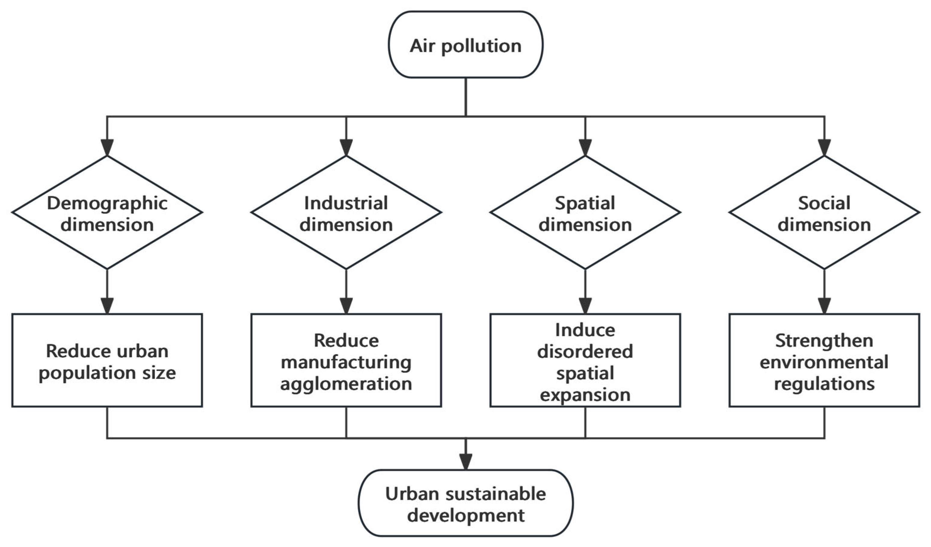
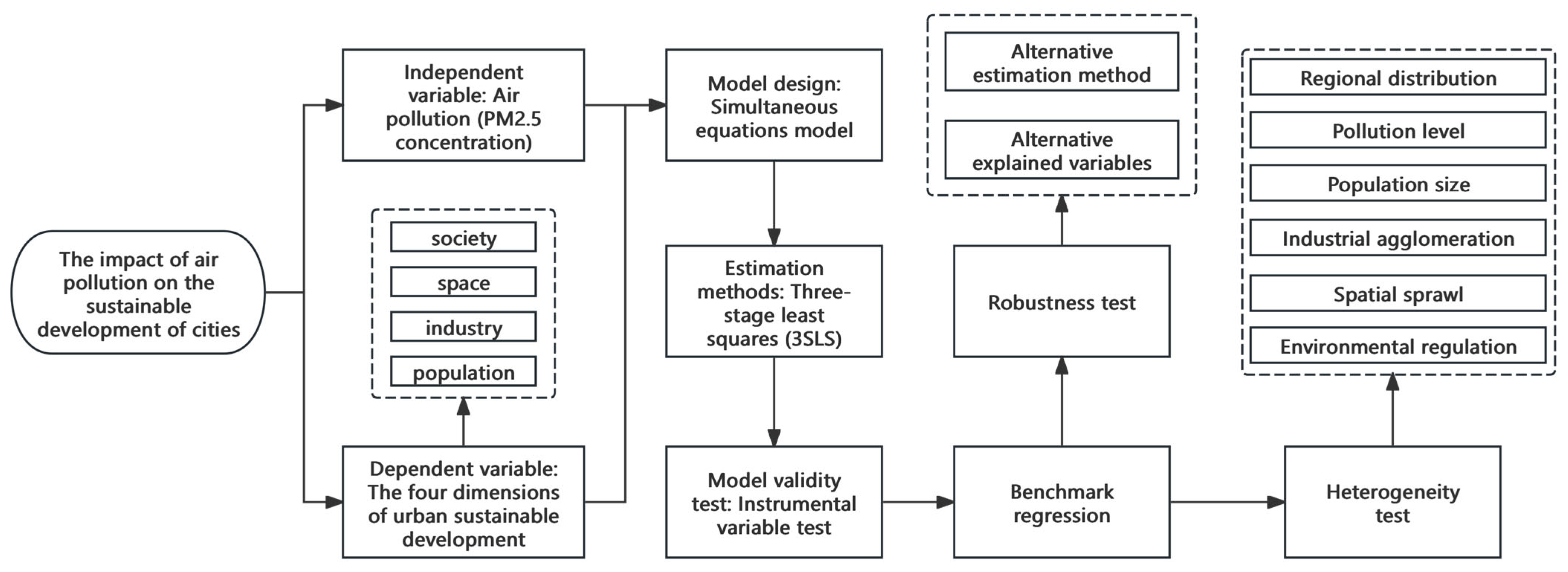
Disclaimer/Publisher’s Note: The statements, opinions and data contained in all publications are solely those of the individual author(s) and contributor(s) and not of MDPI and/or the editor(s). MDPI and/or the editor(s) disclaim responsibility for any injury to people or property resulting from any ideas, methods, instructions or products referred to in the content. |
© 2025 by the authors. Licensee MDPI, Basel, Switzerland. This article is an open access article distributed under the terms and conditions of the Creative Commons Attribution (CC BY) license (https://creativecommons.org/licenses/by/4.0/).