Article

CO Emission Prediction Based on Kernel Feature Space Semi-Supervised Concept Drift Detection in Municipal Solid Waste Incineration Process

1
School of Information Science and Technology, Beijing University of Technology, Beijing 100124, China
2
Beijing Laboratory of Smart Environmental Protection, Beijing 100124, China
*
Author to whom correspondence should be addressed.
Sustainability 2025, 17(13), 5672; https://doi.org/10.3390/su17135672
Submission received: 8 August 2024 / Revised: 3 September 2024 / Accepted: 8 September 2024 / Published: 20 June 2025
(This article belongs to the Special Issue Novel and Scalable Technologies for Sustainable Waste Management)

Abstract

:
Carbon monoxide (CO) is a toxic pollutant emitted by municipal solid waste incineration (MSWI), which has a strong correlation with dioxins. In terms of the sustainable development of an ecological environment, CO emission concentration is strictly controlled by the environmental departments of various countries in the world. The construction of its prediction model is conducive to pollution reduction control. The MSWI process is affected by multi-factors such as MSW component fluctuation, equipment wear and maintenance, and seasonal change, and has complex nonlinear and time-varying characteristics, which makes it difficult for the CO prediction model based on offline historical data to adapt to the above changes. In addition, the continuous emission monitoring system (CEMS) used for conventional pollutant detection has unavoidable misalignment and failure problems. In this article, a novel prediction model of CO emission from the MSWI process based on semi-supervised concept drift (CD) detection in kernel feature space is proposed. Firstly, the CO emission deep prediction model and the kernel feature space detection model are constructed based on offline batched historical data, and the historical data set for the real-time construction of the pseudo-labeling model is obtained. Secondly, the drift detection for the CO emission prediction model is carried out based on real-time data by using unsupervised kernel principal component analysis (KPCA) in terms of feature space. If CD occurs, the pseudo-label model is constructed, the pseudo-truth value is obtained, and the drift sample is confirmed and selected based on the Page–Hinkley (PH) test. If no CD occurs, the CO emission concentration is predicted based on the historical prediction model. Then, the updated data set of the CO emission prediction model and kernel feature space detection is obtained by combining historical samples and drift samples. Finally, the offline history model is updated with a new data set when the preset conditions are met. Based on the real data set of an MSWI power plant in Beijing, the validity of the proposed method is verified.

1. Introduction

Municipal solid waste (MSW) refers to all kinds of solid waste generated in people’s daily production, life and consumption [1]. Long-term accumulation and management lack can easily cause urban living space pollution, occupation, virus transmission, and other hazards [2,3]. The latest World Bank statistics show that in the absence of action on MSW production, global MSW annual production will rise by 70% to 3.4 billion tonnes in 2050 [4]. The rapid growth of MSW production has led to the gradual increase in environmental risks of “Garbage siege” [5], which seriously restricts its sustainable and healthy development [6,7]. The report of China proposed that “building an ecological civilization is a millennium project for the sustainable development of the Chinese nation” and made a strategic deployment to accelerate the reform of the ecological civilization system and build a beautiful China [8], and clearly pointed out that the reasonable disposal of MSW is an important aspect of China’s ecological civilization construction [9].
MSW incineration (MSWI) technology has become the preferred technology for MSW disposal [10,11], which has advantages such as a high-quality reduction rate, high-capacity reduction rate, and energy recycling [12], as well as its potential value in economic and environmental protection [13,14]. At the same time, under the development background of the “carbon peaking and carbon neutrality” strategy, waste classification and “zero landfill” of the original MSW, MSWI is an indispensable part of sustainable development and green environmental protection of large cities [15]. Carbon monoxide (CO), as one of the toxic gases produced in the process of MSWI, is difficult to sense by the senses. When combined with hemoglobin, it will hinder blood oxygen delivery and even cause myocardial infarction in the human body [16,17], so it must be strictly controlled [18].
Due to the unknown uncertainty fluctuation of MSW components, the high-frequency intervention and experience difference of experts in the field in operation, the maintenance and aging of incineration equipment, and other factors, the operating condition of the MSWI process has complex dynamic time-varying characteristics [19]. This is difficult to overcome, and predictable operating condition fluctuation is reflected in the change in the distribution of data flow over time, which is called concept drift (CD) [20,21] in the academic field. Therefore, building a high-precision CO prediction model requires not only determining a suitable modeling algorithm, but also solving how to detect CD and update the historical model with samples that can characterize the drift. Although conventional pollutants, including CO, NOx, SO2, etc., can be continuously detected by the continuous emission monitoring system (CEMS) located at the tail of the chimney, the system has unavoidable misalignment and failure phenomena [22]. The existing CO prediction models for the MSWI process include the method based on reduced depth feature and LSTM optimization [23], the method based on fixed window CD detection [24] and the heterogeneous ensemble prediction model method driven by virtual and real data [25]. However, these methods do not consider the prediction model updating when the CEMS system failure cannot provide the model truth value and CD occurs. Therefore, when updating the CO emission prediction model, it is also necessary to pay attention to how to effectively update the model without the truth value. Therefore, the constructed CO prediction model can replace these models in such a special situation. Moreover, to effectively control the MSWI process, domain experts typically predict changes in CO concentration to adopt more effective ‘air and material distribution’ control. Meanwhile, the CO prediction model is also necessary for realizing the intelligent optimization control of the MSWI process [26]. Therefore, the method proposed in this article not only has the functionality of a CEMS system in terms of CO emission concentration but also provides support for intelligent control and operational optimization of MSWI processes.
CD detection can be divided into two types: supervised and unsupervised [27]. The representative CD detection algorithm is the drift detection method (DDM), which defines the warning and drift levels according to the new sample measurement performance [28]. Frias et al. [29] based their study on the exponential weighted moving average method, and Mahdi et al. [30] based their study on the Page–Hinkley (PH) test method to confirm changes in the model accuracy to determine whether CD has occurred, but it is difficult to directly use the supervised CD detection method in the actual industrial process [31]. The representative algorithm of unsupervised CD detection [32] analyzes the distribution changes in feature space based on principal component analysis (PCA) [33]. The disadvantage of the PCA method is that it does not rely on the truth value in the CD detection stage, but samples labeled with truth value are still needed in the model update stage. It is difficult to make the model adapt to CD in a short period of time [34]. In addition, the influence of CD in complex industrial processes can be reflected in the comprehensive change in terms of output error space and input feature space. In order to make use of the large number of unlabeled samples of the process, the semi-supervised learning method has been used to model the process data. For example, Ji et al. [35] proposed a semi-supervised recursively weighted kernel regression algorithm for soft-sensing modeling of a semi-batch process, and Ge et al. [36] used a semi-supervised Bayesian method for soft-sensing modeling of a large number of unlabeled samples of the process. Zhu et al. [37] proposed a robust semi-supervised mixed rate principal component regression model and applied it to process soft measurement. This method can not only make use of a large number of unlabeled samples but also effectively solve the process outlier problem. Therefore, for the CO emission prediction problems of the MSWI process, it is very necessary to study how to carry out online prediction, real-time drift detection and model updating.
To solve the above problems, this article proposes a CO emission prediction model in the MSWI process based on semi-supervised CD detection in kernel feature space. It can be used to predict CO concentration and achieve emission reduction control of the MSWI process. The main innovations are as follows: (1) a semi-supervised CD detection framework is proposed, including historical CO prediction model and CD detection model construction, real-time CO prediction and CD detection, updated data set acquisition and historical model update modules; (2) an algorithm that uses unsupervised kernel principal component analysis (KPCA) identification to recognize CD in the feature space is proposed. When drift occurs, a pseudo-labeling model is constructed in real time to obtain pseudo-truth values, and drift samples are confirmed based on a PH test. (3) The updated data set of the model is obtained by combining historical samples and drift samples, and the strategy of using a new data set to update the historical model when the preset conditions are met is proposed.
The rest of the organizational structure of this article is arranged as follows. Section 2 describes the material and method, including the MSWI process for CO emission concentration, the overall algorithm and the implementation of the algorithm. In Section 3, the experimental research is carried out based on industrial application. Section 4 summarizes the research.

2. Materials and Methods
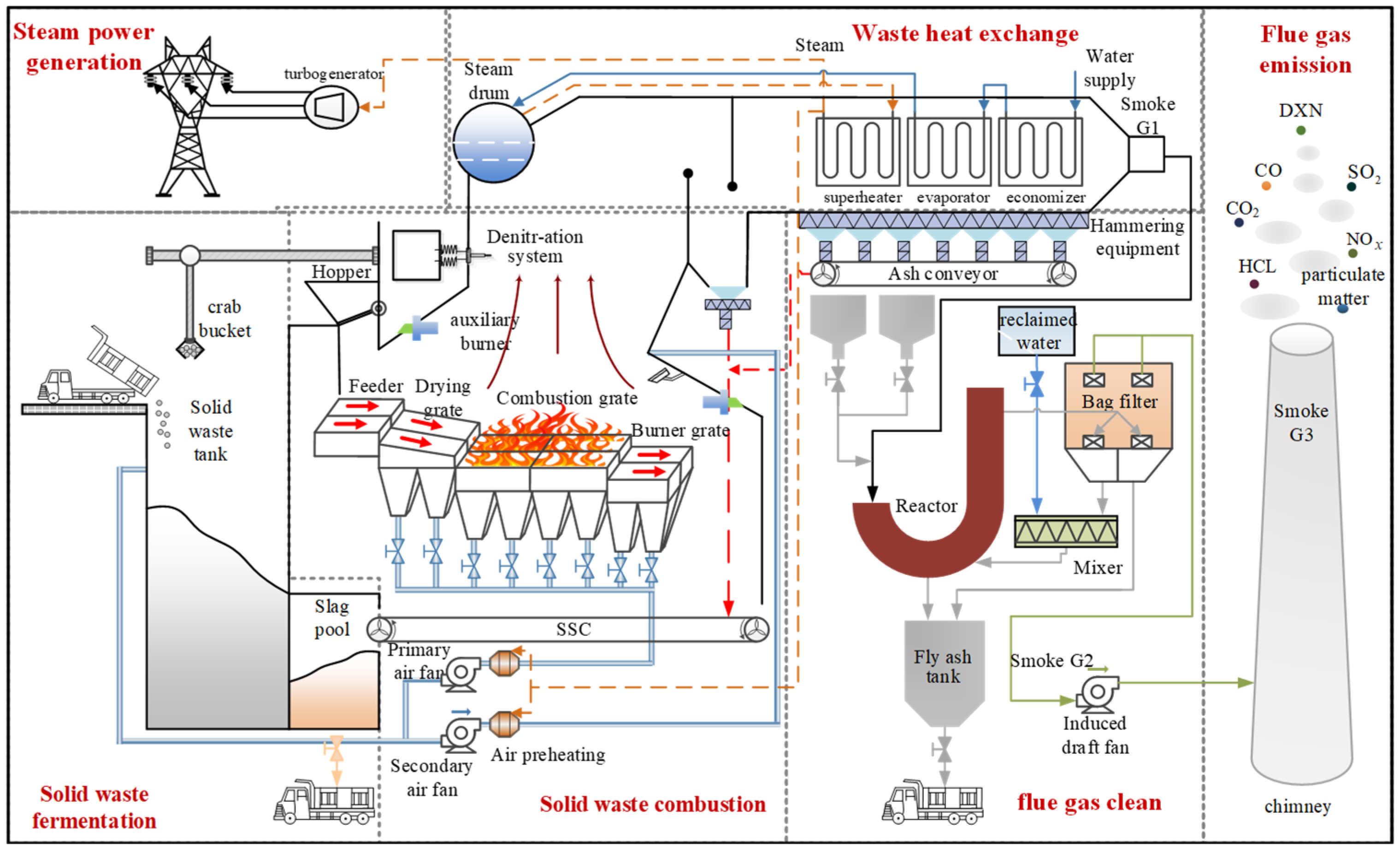
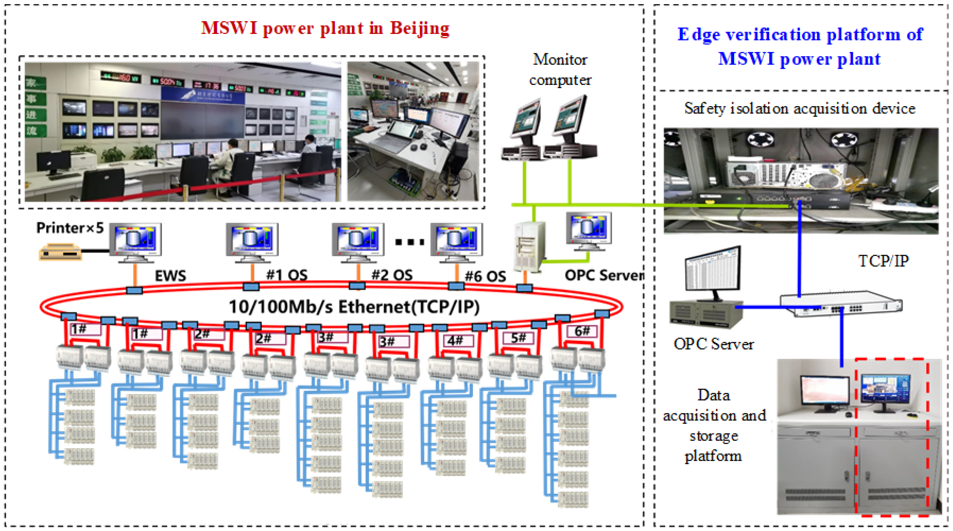
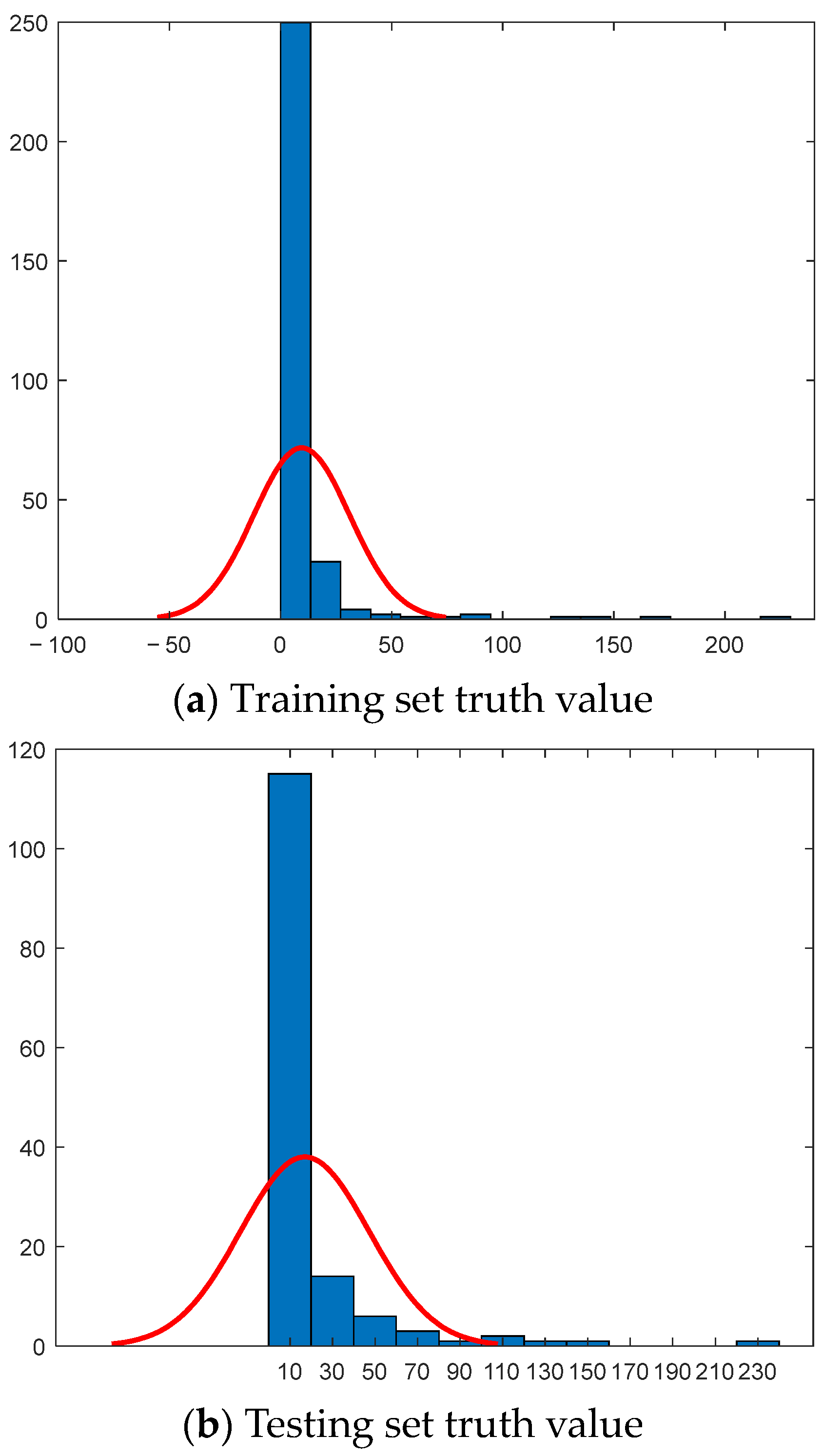
2.1. Materials

The process flow of a typical grate furnace MSWI is shown in Figure 1. It mainly includes six process stages: solid waste fermentation, solid waste combustion, waste heat exchange, flue gas cleaning, flue gas emission, and steam power generation [38].
For solid waste combustion, due to insufficient oxygen supply (part of the MSW cannot be completely oxidized), uneven combustion (part of the MSW cannot be fully exposed to oxygen) or insufficient temperature (insufficient incineration temperature, combustion reaction rate is reduced), the MSW will undergo incomplete combustion, resulting in the generation of CO. Therefore, the change in furnace temperature, flue gas oxygen content and other factors cause the CD in terms of CO emission concentration.
The traditional MSWI process can detect the CO emission concentration in real time through the CEMS [1], which is usually measured by full extraction or dilution extraction. However, when full extraction is carried out, it is easy to clog the extraction port in a positive pressure environment or when the extraction volume is too large. During dilution extraction, the measurement response is too long and the purity of dry compressed air is required to be high. In addition, CEMS has failure problems and requires qualified technicians to carry out regular maintenance [39]. Therefore, it is necessary to label the pseudo-truth values to analyze the CD phenomenon in the process when the truth values cannot be obtained.
Some detailed information about an MSW plant in Beijing is as follows. The capacity of MSW is 628.8 t/d. The length of the grate is 11 m and the width is 12.9 m. The airflow of the primary is 67,500 m3/h. The temperature of the air is 200 °C. Primary air enters the bed from four independent parts of the grate below. The flow rate of each part accounts for 24.31%, 43.35%, 19.27% and 13.07% of primary air, respectively.
The data was collected through an edge verification platform of an MSWI power plant equipped with a safety isolation acquisition device. The device facilitates one-way data transmission, mitigating interference issues during the data acquisition process, as shown in Figure 2.
Monitoring and responding to concept drift can help ensure that models remain accurate and reliable in dynamic environments such as the MSWI process. Concept drift is often manifested as a change in data distribution. It is assumed that all historical samples obey F 1 , t Htd , and new time samples obey F k Otd ; if F 1 , t Htd = F k Otd , no drift occurs, and vice versa, F 1 , t Htd F k Otd , drift occurs. In this article, the CO emission prediction model of the MSWI process is constructed. In total, 36 h of data were taken, and the average value of 5 min was taken as one sample for the final data, totaling 432 samples. The first two-thirds of the data set is divided into the training set and the last third into the testing set.
Figure 3 shows the histogram of CO emission concentration data in the actual MSWI process, which is represented by a series of longitudinal stripes or line segments with varying heights. Generally, the horizontal axis indicates the data type, and the vertical axis indicates the distribution.
According to the truth distribution of the training and testing sets, there are big differences in the distribution. It indirectly reflects the phenomenon of CD in the data set of the actual MSWI process.

2.2. Methods

The CO emission prediction strategy based on kernel feature space semi-supervised concept drift detection proposed in this article is shown in Figure 4.
The functions of each module of the proposed strategy are described as follows:
(1)
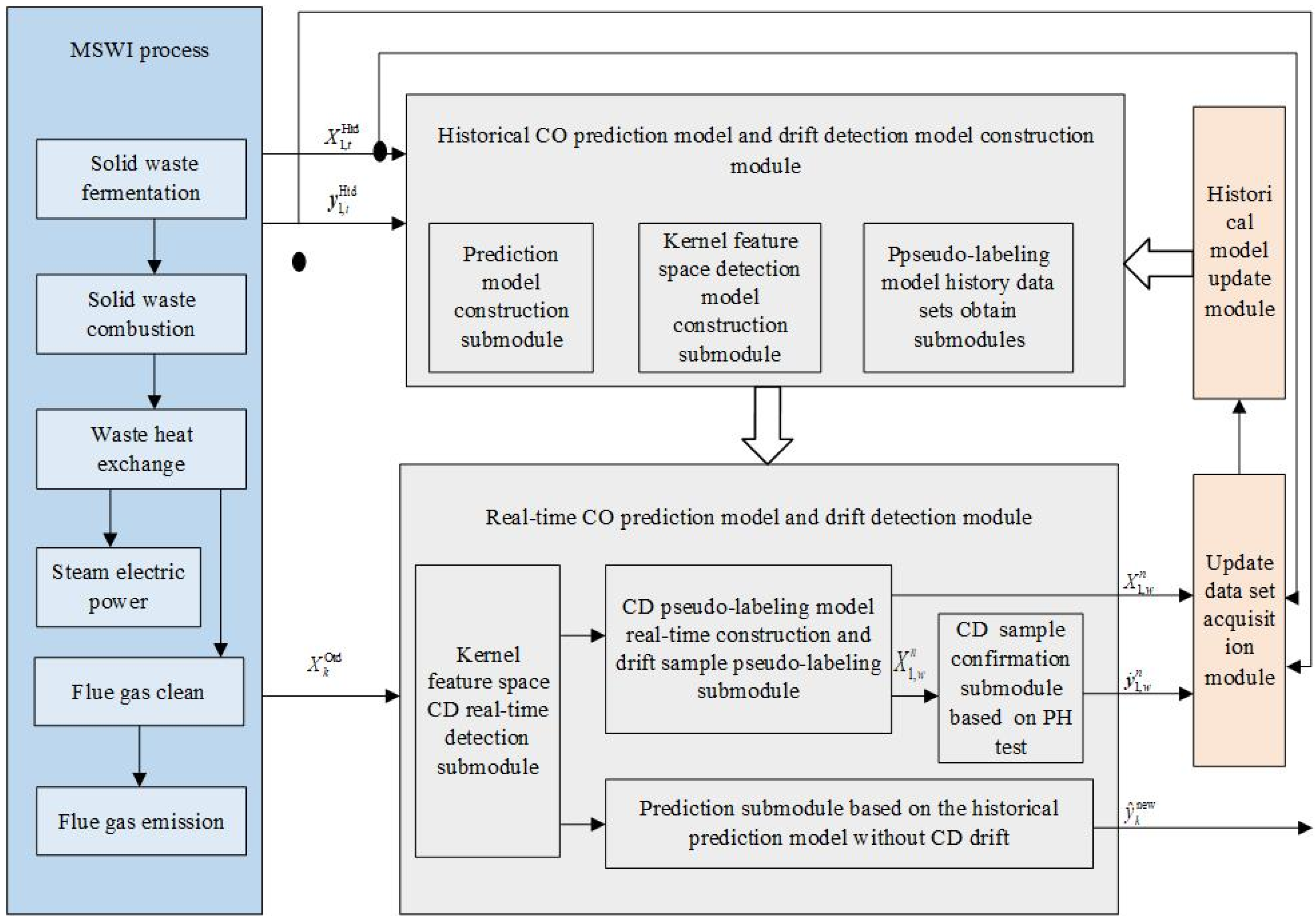
Historical CO prediction model and drift detection model construction module: historical samples are used to build prediction models and kernel feature space detection models and to obtain historical data sets to support pseudo-labeling model construction.
(2)
Real-time CO prediction model and drift detection module: When the CD detected value exceeds the KPCA control limit, it is considered that the sample has a drifting possibility. At this time, the sample is stored in the cache window to be labeled. When the number of samples in the window reaches the preset window capacity, a pseudo-labeling model is constructed in real time, and the drift samples are marked with pseudo-truth values. For the pseudo-truth values after labeling, the PH test method was used to determine whether the samples were drifting. If no CD occurs, the CO emission concentration is predicted based on the historical prediction model.
(3)
Update data set acquisition module: the samples confirmed to drift in the current cache window are recorded as the drift sample data set, and the historical data set is determined according to experience for the model update.
(4)
Historical model update module: The acquired updated data set is retrained for the CO prediction model and kernel feature space detection model, and the historical data set of the pseudo-labeling model is updated. At the same time, the cache window to be labeled is reset.

2.2.1. Historical CO Prediction Model and Drift Detection Model Construction Module

Prediction Model Construction Submodule

The purpose of model learning is to determine the CD prediction model with the minimum prediction error f LSTM Htd . The structure of the used LSTM is as follows Figure 5.
The output of the LSTM-based CO emission prediction model constructed with offline samples can be expressed as follows:
y ^ Htd = f LSTM Htd X std Htd

Kernel Feature Space Detection Model Construction D n Submodule

For high-dimensional process variables, the KPCA model is used to calculate the CD detection control limit for determining whether the MSWI process changes. At first, the historical training data is denoted as X std Htd . Then, we map the vector x Htd in X std Htd to a higher-dimensional space F (denoted as dimensional) as follows:
ϕ x Htd :   R M R D ,   D M
where ϕ is a nonlinear mapping function, and D is the mapped data dimension.
The high-dimensional mapping space is represented as follows:
ϕ X std Htd = ϕ x 1 Htd ,   ϕ x 2 Htd , ,   ϕ x N Htd
Then, the kernel function is introduced to calculate the kernel matrix (K). This article uses the sigmoid kernel function as follows:
K = f β 0 X std Htd X std Htd T + β 1
where f uses the tanh function, β 0 and β 1 user-defined. Generally, β 1 is set as 0 by default.
By defining 1 N as 1 matrix, the kernel matrix is centralized as
U = 1 N N
Then, the kernel matrix (Kc) after centralization is calculated as follows:
K c = K N   ×   N U N   ×   N K N   ×   N K N   ×   N U N   ×   N + U N   ×   N K N   ×   N U N   ×   N
In this article, the eigenvalue decomposition method is used to solve the eigenvalue and eigenvector of the matrix, and the calculation is as follows:
K c N = Q Σ Q 1
where Q is the eigenvector matrix and Σ = d i a g λ 1 , λ 2 , , λ N is the diagonal matrix. In K c = K N   ×   N U N   ×   N K N   ×   N K N   ×   N U N   ×   N + U N   ×   N K N   ×   N U N   ×   N , each element on the diagonal is an eigenvalue.
The eigenvalues are normalized and calculated as follows:
Q s = Q N λ T
where Q s is the matrix normalized by Q , and λ is the eigenvector.
The cumulative feature contribution rate ( η ) and KPCA contribution threshold δ KPCA were used for the selection of the number of principal components, which are as follows:
η = p = 1 p λ p m = 1 M λ m
where p is the number of selected principal components, M is the eigenvector number of X Htd , and p is less than M .
Accordingly, the CD detection control limit for monitoring whether the operating condition changes is determined by P.
The nonlinear principal components are calculated by the obtained kernel principal components, which are shown as follows:
P = K c Q s _ p
where Q s _ p is the matrix of size N × p in Q s , and P is a nonlinear principal component matrix with size N × p .
Statistical indicators T 2 and S P E according to Hotelling are adopted as the control limits for the identification of operating condition drift. They are expressed as
( T α 2 ) Htd = p ( N 1 ) ( N p ) F α p , N p
S P E α Htd = θ 1 c α 2 θ 2 h 0 2 θ 1 + 1 + θ 2 h 0 ( h 0 1 ) θ 1 2 1 / h 0
where F α ( p , N p ) is an F distribution with p and ( N p ) degrees of freedom and c α represents the normal deviation from the upper ( 1 α ) percentile. θ i and h 0 are calculated as follows:
h 0 = 1 2 θ 1 θ 3 / 3 θ 1 2
θ i = m = p + 1 M λ m i , i = 1 , 2
Therefore, the historical CD detection model is constructed f KPCA Htd .

Pseudo-Labeling Model History Data Sets Obtain Submodules

The first-order difference components of each sample in error output and feature space in the historical sample set ( X 1 , t Htd ) are calculated. By taking sample x t Htd as an example, they are calculated as follows:
Δ x t Htd = x t Htd x t 1 Htd
Δ y t Htd = y t Htd y t 1 Htd
where x t Htd and x t 1 Htd represent the feature space of the sample respectively; y t Htd and y t 1 Htd represent the true value of the sample, respectively.
According to Equations (15) and (16), the data set of first-order difference components of the error output space and the feature space of the historical sample is denoted as Δ y Htd and Δ X Htd , respectively.

2.2.2. Real-Time CO Prediction Model and Drift Detection Module

Kernel Feature Space CD Real-Time Detection Submodule

In this article, we denoted the testing data as X k Otd . Firstly, the vector x k Otd in X k Otd is mapped to a higher-dimensional space F , and the kernel function is introduced to calculate the kernel matrix K t (size N k × N ). The used Sigmoid kernel function in terms of testing data is denoted as
K t = f β 0 X k Otd X Htd T + β 1
where f uses the tanh function.
By defining N k × N 1-matrix with size N k × N as 1 N k , the kernel matrix is centralized as
U t = 1 N k N
Then, the kernel matrix ( K t _ c ) after centralization is calculated as follows:
K t _ c = K t N k × N U t N k × N K N × N K t N k × N U N × N + U t N k × N K N × N U N × N
where the size of K t _ c is N k × N .
The kernel principal components in terms of testing data are calculated based on the obtained number of principal components, which are shown as follows:
P t = K t _ c Q s _ p
where Q s _ p is the matrix of size N × p , and P t is a matrix of size N k × p .
The CD detection value of the new sample is calculated as follows:
T k 2 = d i a g P t d i a g λ p P t
S P E k = K t _ c Q s 2 P t
According to whether T k 2 and S P E k of the samples in the window meet the following criterion, determine whether CD occurs.
Drift , i f   T k 2 > ( T α 2 ) Htd   or   S P E k > S P E α Htd Normal , other

Prediction Submodule Based on the Historical Prediction Model without CD Drift

If no drift occurs, the prediction of CO emission concentration is made based on the historical prediction model f LSTM Htd . The prediction results are denoted as follows:
y ^ k new = f LSTM Htd X k Otd

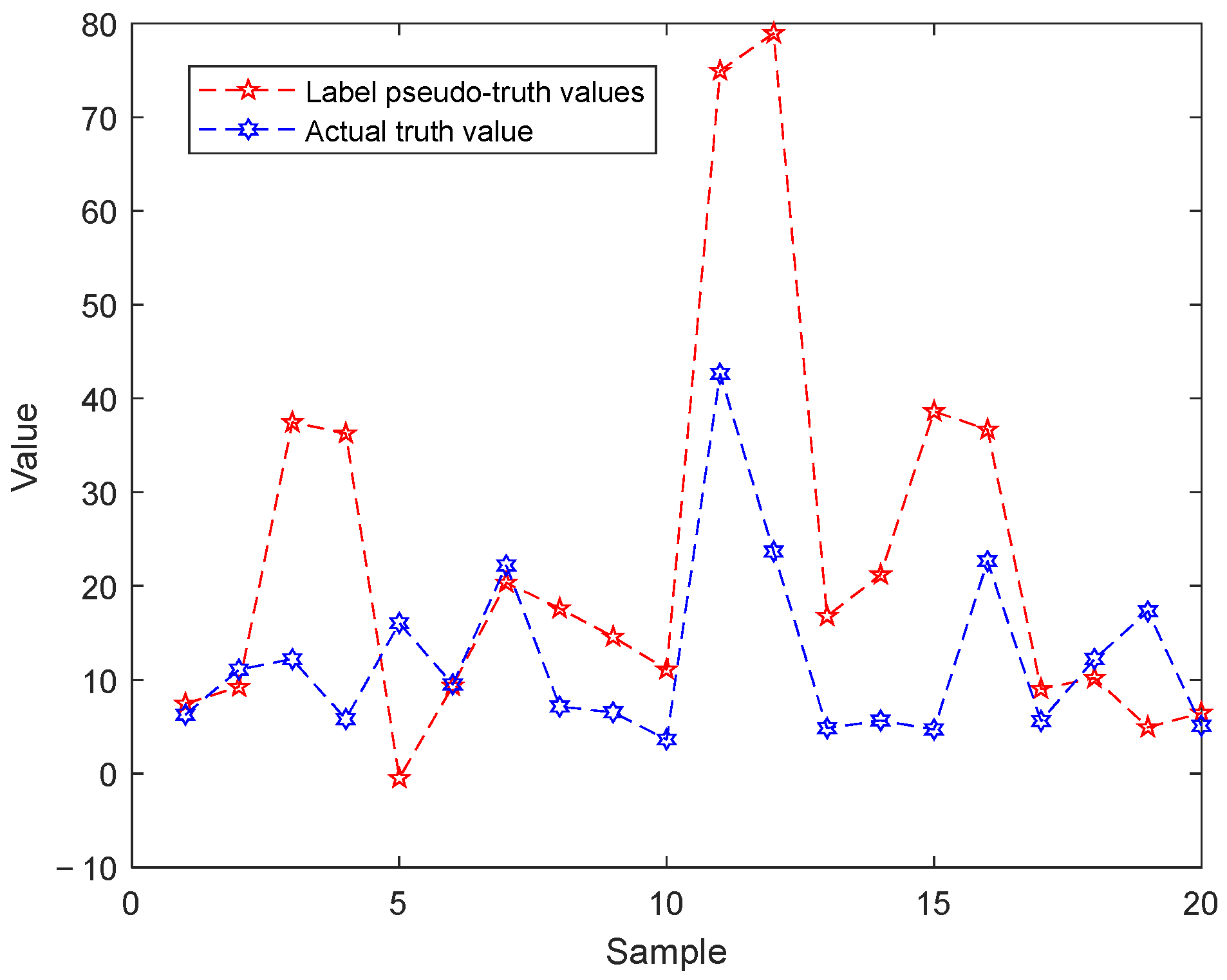
CD Pseudo-Labeling Model Real-Time Construction and Drift Sample Pseudo-Labeling Submodule

After KPCA filtering and the cache window to be labeled is filled, the sample set in the window is denoted as X window   = x 1 window   , , x w window   , where w is the preset cache window sample capacity. The detailed pseudo-labeling process is as follows.
Firstly, a new set of first-order difference components is constructed as
Δ y Htd = Δ y Htd Δ y 1 window  
Δ X Htd = Δ X Htd Δ X 1 window  
where y 1 window   and X 1 window   are truth value and feature space, respectively; Δ y 1 window   and Δ X 1 window   are the first-order difference components obtained by x 1 window   and the last time samples in the current training set.
By starting from x 2 window , we calculate the first-order difference component of its feature space X 1 window as follows:
Δ X 2 window   = X 2 window   X 1 window  
Based on the idea of nearest neighbor, ε feature space difference components with the smallest distance between Δ X Htd and Δ X 2 window   are selected from Δ X Htd through Euclidean distance. By combining with their corresponding output space difference components, they are written as
Ω nearest = Δ x nearest _ 1 Htd , Δ y nearest _ 1 Htd , , Δ x nearest _ ε Htd , Δ y nearest _ ε Htd
Based on Ω nearest , the pseudo-labeling model based on LSTM is established. The error output space difference component Δ y ^ 2 window of x 2 window is obtained as the following steps,
Ω nearest LSTM nearest
LSTM nearest Δ X 2 window   Δ y ^ 2 window  
Then, the pseudo-truth value y ˙ 2 window of x 2 window is calculated and denoted as
y ˙ 2 window   = Δ y ^ 2 window   + y 1 window  
Repeat the above process until the samples in the window are labeled with pseudo-truth values.

CD Sample Confirmation Submodule Based on PH Test

A reasonable analysis of the difference between the pseudo-truth value of the sample and the measured value is the key to confirming the sample CD. In the PH test method, given a series of observations [ l 1 , l 2 , l m ] , the likelihood ratio statistic of the alternative hypothesis (there is a CD point γ in the observations, that is, 1 < γ < m ) against the null hypothesis (there is no drift in the observations, that is, γ > m ) is calculated as [39]
L m , γ = i = 1 γ f D l i i = γ + 1 m f D l i δ i = 1 m f D l i
where i = m + 1 m f D l i = 1 , i = m + 1 m l i = 0 ; f D represents the distribution density function of the standard normal distribution N ( 0 , 1 ) ; and δ means that the CD sample follows a normal distribution with a mathematical expectation of δ .
The above Equation is expressed logarithmically as
Z m , γ = ln L m , γ = δ i = γ + 1 m l i δ 2
Accordingly, the log-likelihood ratio statistic of the alternative hypothesis (with CD) to the null hypothesis (without CD) is
Z m = max 1 γ < m Z m , γ = max δ i = γ + 1 m l i δ 2
By setting a threshold and comparing it with Z m , we can determine whether CD exists in the current series of pseudo-truth values.
When all samples in the cache window to be labeled are marked with pseudo-truth values, this article adopts the PH test method to detect CD in the error output space of these samples. By taking the observed value Obs(t) at time t as an example, the detection process is as follows:
First, we calculate the cumulative variable φ t for Obs(t):
O b s ¯ t 1 = 1 t 1 m = 1 t 1 O b s ( m )
φ t = m = 1 t ( O b s ( m ) O b s ¯ m 1 )
where O b s ¯ t 1 represents the mean of all historical observations at the previous t − 1 moment; φ t represents the difference between the current observation Obs(t) and the mean historical observations.
Then, the change index PHt is calculated to determine whether the current observed value Obs(t) is abnormal:
ϕ t = min m = 1 t φ m
P H t = φ t ϕ t
where ϕ t represents the minimum cumulative variable value recorded from all current moments; P H t represents the difference between the cumulative variable φ t and the minimum cumulative variable value at the current time t . When condition P H t > λ  is satisfied, the observed Obs(t) is considered abnormal, where λ is the empirical threshold.
The sample set in the window is denoted as X window d = x 1 d , , x w d when the cache window to be labeled is filled for the d time and all samples are labeled. We calculate the sample average measurement error ( A v e e r o d ) in the current window as follows:
A v e e r o d = 1 w m = 1 w y ^ m d y ˙ m d
where y ^ m d and y ˙ m d represent the true and pseudo-true values of the mth sample in the window, respectively.
On this basis, this article selects the observed value Obs(t) as the cumulative average measurement error of the samples in the window when the window is filled d times, namely
O b s ( t ) | t = d = O b s ( t 1 ) ( d 1 ) + A v e e r o d d ( d 1 )
In this case, the cumulative variable ( φ t ) represents the difference between the current cumulative average prediction error and the mean historical cumulative average prediction error. We denote ϕ t as the minimum φ t value of the current record. When the cache window is filled for the first time, that is, when d = 1 and ϕ t = φ t . In this case, there is no basis for judging CD in the sample error output space, so this article represents ϕ t as
ϕ t | t = d = min m = 1 t φ m , d 1 ϕ 0 , d = 0
where ϕ 0 is the benchmark cumulative average measurement error, which is obtained according to the average measurement error of the verification sample. At the same time, this article sets λ = 0 , that is, when φ t > ϕ t , which represents that the cumulative average prediction error in the next window is significantly higher than that in the historical sample, it is considered that the sample in the window can represent the CD, and it is used to construct a new training set.

2.2.3. Update Data Set Acquisition Module

When the samples in the cache window are confirmed to drift, this article builds a new training set based on the historical samples and the samples in the current window to update the prediction model. By taking the sample X window d in the window when the cache window is filled for the d time as an example, a new training set ( X d newtd ) is constructed as follows:
X d newtd = X 1 , t Htd X 1 , w n
y d newtd = y 1 , t Htd y ˙ 1 , w n
where X d newtd and y d newtd are the input feature space and truth value of the updated data set, respectively; X 1 , w d and y ˙ 1 , w d are the input feature space and the pseudo-truth of the samples in the current window, respectively.

2.2.4. Historical Model Update Module

The updated data set is used to construct the CO prediction model and the kernel feature space CD detection model. The output of the new prediction model for CO emission based on LSTM by using X window d can be expressed as follows:
y ^ New newtd = f LSTM new X d newtd
The KPCA-based CD model can be expressed as follows:
{ T new 2 , S P E new , } = f KPCA new X d newtd
Replace the original model with a new mode and update the pseudo-token model history data set at the same time as follows:
f LSTM Htd f LSTM new f KPCA Htd f KPCA new Δ X Htd X d newtd Δ y Htd y d newtd
After the above update, the proposed prediction model can better adapt to the dynamic changes in the MSWI process.

2.3. Pseudo-Code

The pseudo-code of the pseudo-code algorithm used in this article is as follows Table 1:

3. Results and Discussion

3.1. Performance Metrics

The evaluation index used in the article is RMSE. The former is calculated as follows:
R M S E = n = 1 N y n y ^ n 2 N

3.2. Experimental Results

3.2.1. Historical Model Construction

The CO prediction model adopts the LSTM model, which has 128 hidden layer units, 210 training times, 0.022 learning rate, 0.2 learning drop factor and 0.4 dropout rate.
Figure 6 shows a graph of the absolute value error of the training set. The horizontal axis shows the number of samples, and the vertical axis shows the absolute error predicted by the sample. The LSTM model has a certain effect on the construction of training samples in process data sets, and the error is small. Therefore, LSTM can be used to effectively build a CO emission prediction model.
The principal component contribution threshold of KPCA was set as 0.91, and five principal components were selected as the principal space for running CD detection. The calculated T2 and SPE control limits are 9.4707 and 0.4246, respectively.
The curve of Δ y Htd in the pseudo-labeling model historical data set is shown in Figure 7.
The horizontal axis represents the number of samples, and the vertical axis represents the first-order difference component predicted by the sample. Figure 7 shows that most of the truth difference components are small, which shows that the method has a certain reliability.

3.2.2. Real-Time Prediction and CD Detection

The T2 and SPE results based on KPCA CD detection are shown in Figure 8. The horizontal axis represents the number of samples, and the vertical axis represents the concept drift detection index T2 and SPE calculated by this sample.
In this article, the window size is set as 3, and the parameters of the constructed pseudo-labeling LSTM model are the same as the constructed CO prediction model. The number of historical samples selected by Euclidean distance is 15. The comparison between the pseudo-truth labeling results and the actual truth values based on TD learning is shown in Figure 9. The horizontal axis represents the number of samples, the vertical axis represents the calculated value of this sample, the red line represents the pseudo-truth value, and the blue line represents the actual truth value.
Figure 9 shows that the variation trend in the pseudo-truth value is similar to the sample truth value. When the sample truth value is difficult to obtain completely, the pseudo-truth value can be used to approximate the CD in the sample error output space.
After the pseudo-truth value labeling of the samples with kernel feature space drift is completed, the PH test is used to detect the pseudo-label drift, as shown in Figure 10.
The horizontal axis represents the number of cache windows filled, and the vertical axis represents the cumulative average measurement error of samples within the window. Figure 10 shows the change in the cumulative average measurement error of samples in the window after each time the cache window to be labeled is filled, and the samples are labeled with pseudo-truth values. Among them, the cache window to be labeled is filled 10 times, and the cumulative average measurement error of samples in the window increases significantly in terms of CD. It becomes stable with the continuous update of the model, indicating that the proposed algorithm can effectively detect CD changes in the sample error output space.

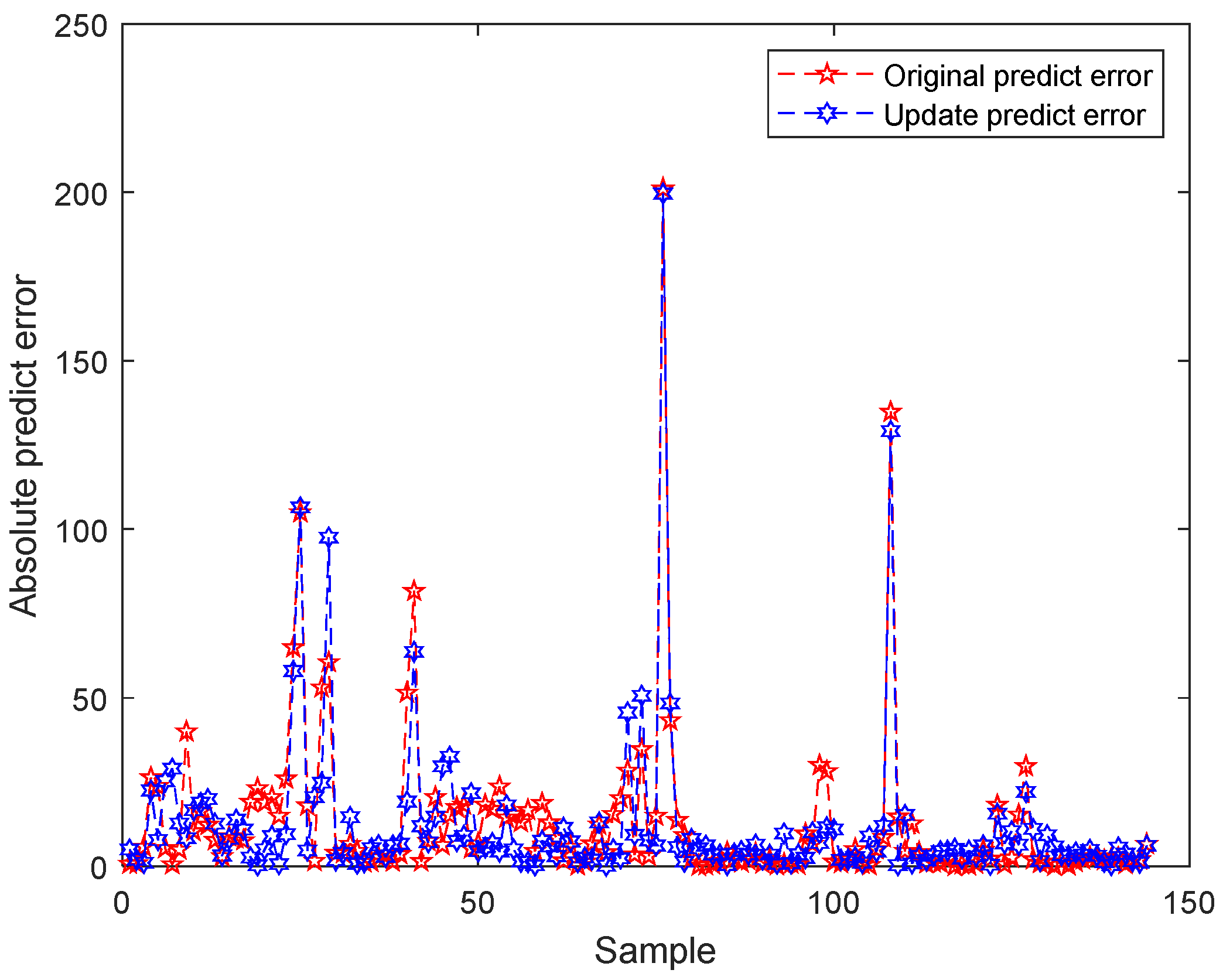
3.2.3. Data Set and Model Update

According to the above test results, after the model is updated with a new training set composed of CD samples and historical samples, the predicted performance changes are shown in Figure 11. The horizontal axis indicates the number of samples, and the vertical axis indicates the absolute measurement error. The red line shows the original measurement error, and the blue line shows the measurement error after updating the model.
The above results show that the prediction error of the proposed CD detection algorithm in the prediction model is significantly reduced compared with the original historical model. Thus, the proposed algorithm can significantly improve the measurement performance of the model in the face of CD drift samples when the truth values of most drift samples are not labeled and can effectively improve the generalization performance of the CO emission prediction model in the MSWI process in the operating condition drift environment.

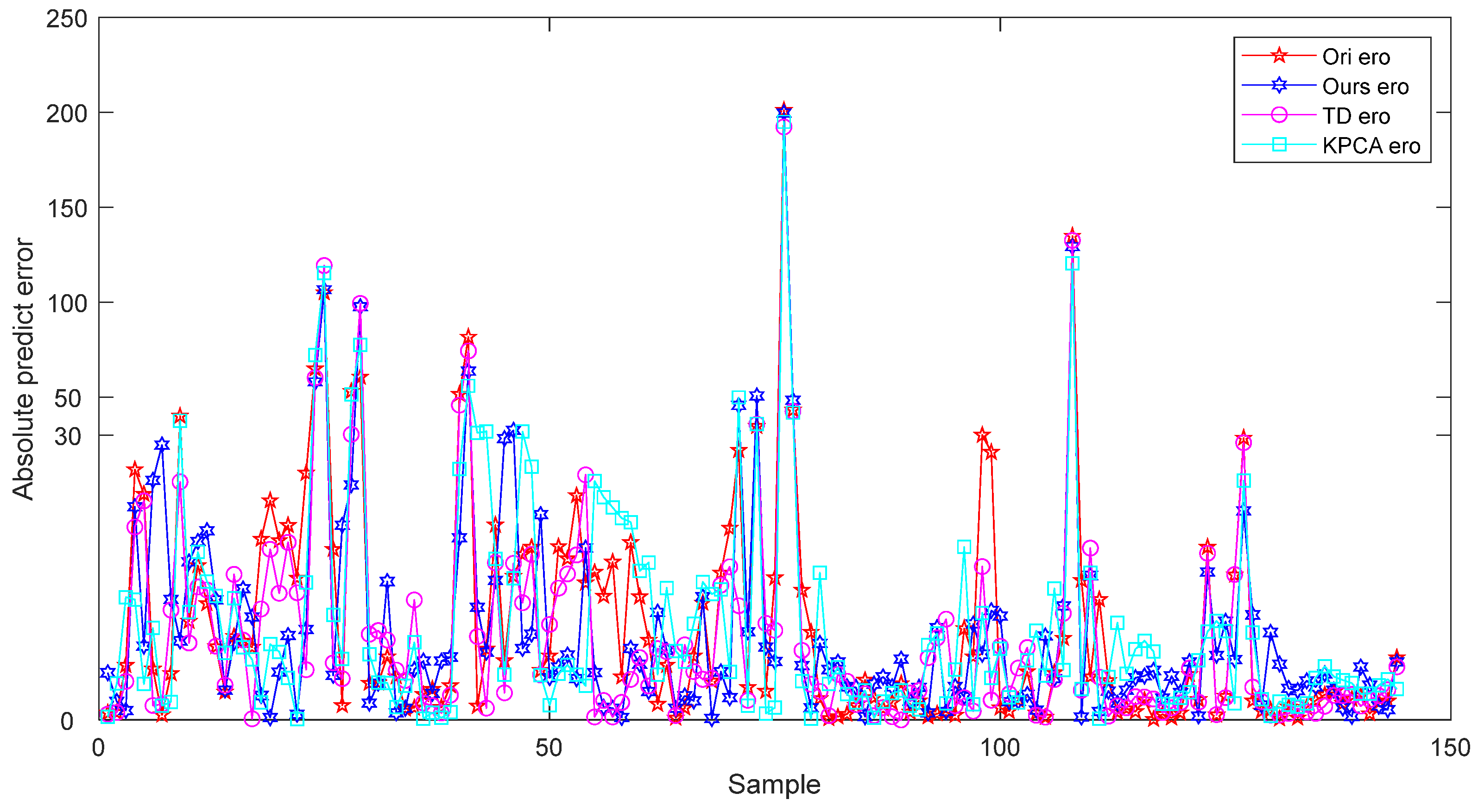
3.3. Method Comparison

In this article, each method was run 30 times, and the optimal results were selected, as shown in Table 2. The predicted curves of different modeling methods are shown in Figure 12.
The horizontal axis indicates the number of samples, and the vertical axis indicates the absolute measurement error. The red line is the original measurement error, and the remaining color lines are the measurement error of the predicted value corresponding to the different models. Table 2 and Figure 11 show that the proposed method has few updating times and the optimal model performance. It can satisfy the CO prediction of the MSWI process when the CEMS system used for conventional pollutant detection has unavoidable misalignment and fault phenomenon.

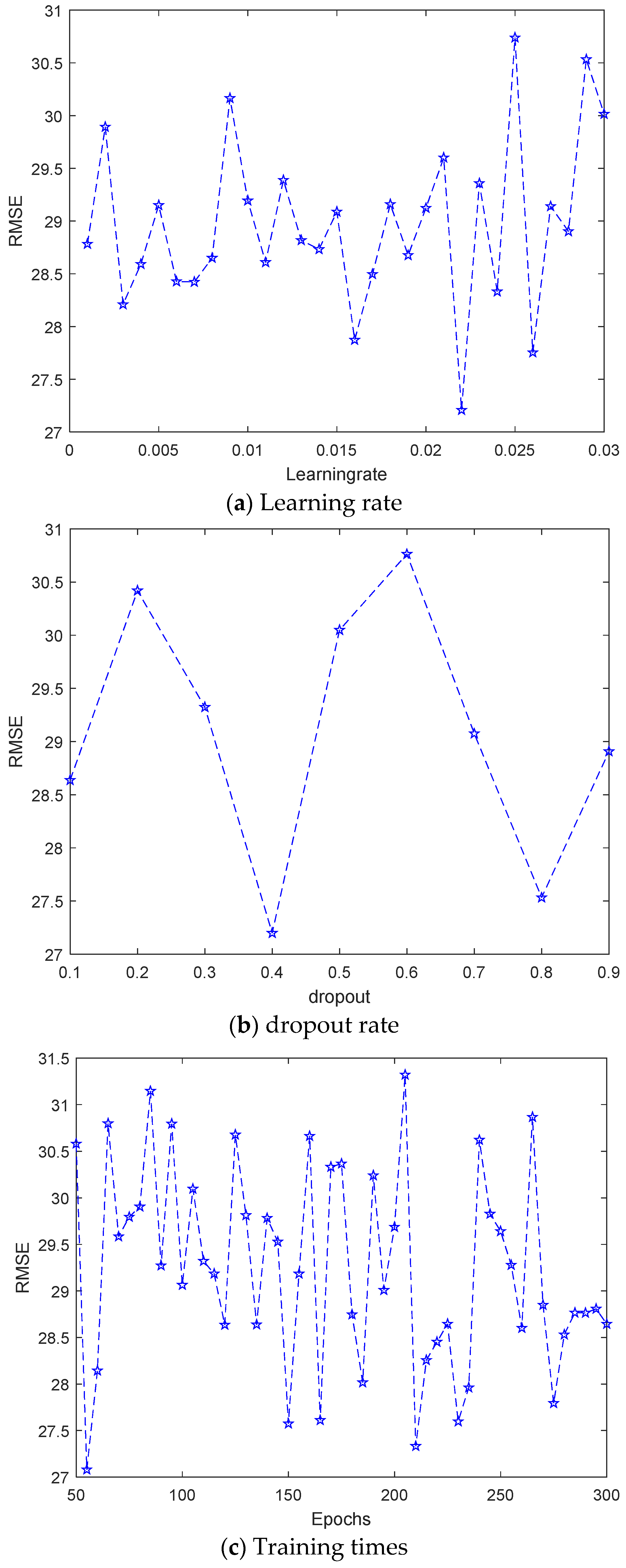
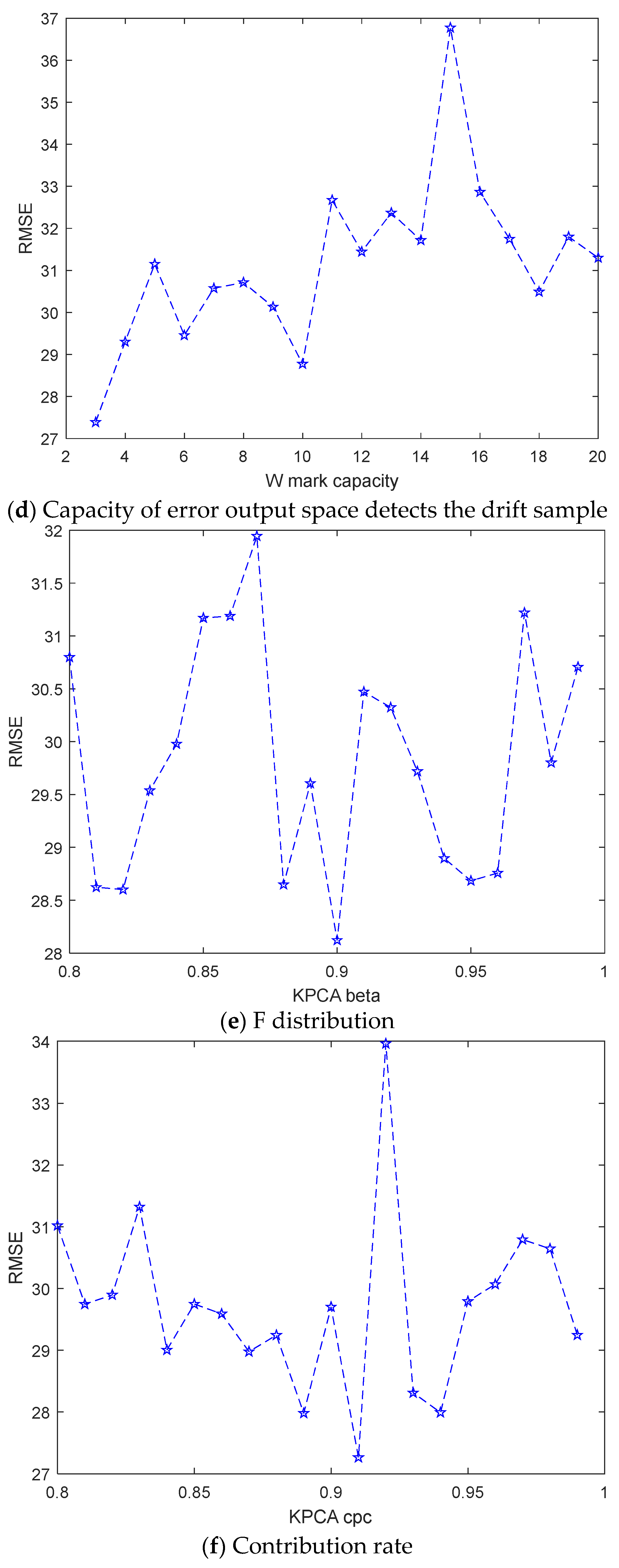
3.4. Hyperparameter Analysis

This section analyzes the sensitivity of hyperparameters of the proposed method in terms of the RMSE index. The setting ranges of hyperparameters are shown in Table 3, and the relationship between them and the RMSE index is shown in Figure 13. The horizontal axis represents the value of the hyperparameter, and the vertical axis represents the RMSE.
Figure 13 shows that
(1)
Learning rate: increasing this value can make the prediction model better fit the training data, and its change will cause fluctuations in the model performance, and 0.022 is preferable;
(2)
Dropout rate: both the training and test accuracy fluctuate within a small range with the change in this value, which is set to 0.4 in this article;
(3)
Training times: the predictive performance of the model is slightly worse with the increase in this value, and the model has the best performance when its value is 210;
(4)
The capacity of error output space detects the drift sample: the prediction performance of the model is slightly worse with the increase in this value, which is set to 3 in this article;
(5)
F distribution: With the setting of the F distribution rate, the model performance fluctuates greatly. In order to ensure the modeling performance, 0.9 is preferred;
(6)
Contribution rate: the smaller the number of selected features, the more appropriate contribution rate should be selected, which is 0.91 in this article.
In addition, considering the coupling between these hyperparameters, the multi-hyperparameter collaborative selection algorithm that can perform global optimization needs further research.

4. Conclusions

To solve the problem of CD in complex industrial processes and the difficulty of obtaining the truth value of predicted key process parameters in real-time, a prediction model of CO emission in the MSWI process based on semi-supervised CD detection in kernel feature space is proposed. The contribution of the proposed method is as follows: (1) the strategy of combining KPCA and PH test fully reflects the CD behavior of new samples in the input feature space and error output space; (2) the semi-supervised mechanism based on TD learning is used for pseudo-labeling of input feature space CD samples, which provides a new method for semi-supervised CD detection for industrial regression problems; (3) the feasibility of the proposed method in practical application is verified by using real MSWI process data set, and the performance of the proposed method is superior to that of the existing methods.
The limitations and potential problems include the following: (1) difficulty in selecting suitable kernel functions for KPCA and being able to update kernel functions based on data changes; (2) updating mixed pseudo-labeling modeling samples in the presence of truth values to improve model performance is not considered; (3) the processing of missing data and outliers in the actual MSWI process is not considered, and the generalization ability should be improved further.
Further research works include the following: (1) to improve the pseudo-labeling algorithm to improve the accuracy of labeling by using use auxiliary information or models; (2) in order to improve the accuracy of the prediction model in practical industrial applications, the mechanism of screening historical modeling samples and mixed pseudo-label modeling samples, and the processing of missing data and outliers would be considered, and a balancing strategy of these two types of samples should be addressed; (3) to determine the best time for model updating based on concept drift amplitude and time may be used in the further researches.

Author Contributions

Conceptualization, T.W.; Methodology, J.T.; Validation, T.W.; Formal analysis, J.T.; Investigation, R.Z.; Resources, R.Z.; Data curation, T.W.; Writing—original draft, R.Z.; Writing—review & editing, J.T.; Supervision, J.T. All authors have read and agreed to the published version of the manuscript.

Funding

This research received no external funding.

Institutional Review Board Statement

Not applicable.

Informed Consent Statement

Not applicable.

Data Availability Statement

The original contributions presented in the study are included in the article, further inquiries can be directed to the corresponding author.

Conflicts of Interest

The authors declare no conflict of interest.

Abbreviations

SymbolMeaning
f LSTM Htd 
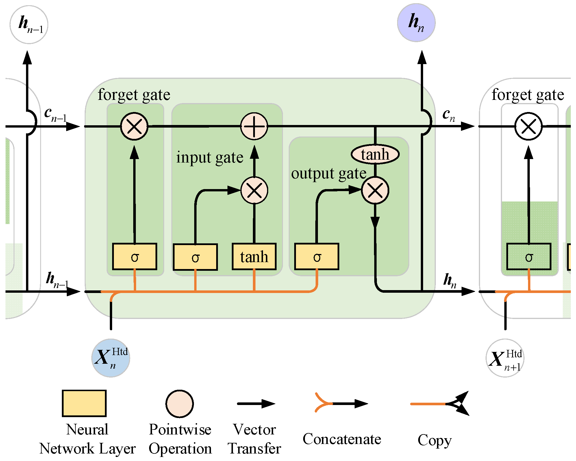
LSTM model built on the basis of historical data is also the prediction model used when there is no drift
X n Htd The n th sample serves as the input to the LSTM
h n LSTM hidden layer output of the n th sample
C n LSTM output status information of the n th sample
σ Sigmoid activation function
Hadamard product
tanh Tanh activation function
U f , U i , U c , U o Weights of the forgetting gate, input gate and output gate correspond to h n 1 , respectively
W f , W i , W c , W o Weights of the forgetting gate, input gate and output gate correspond to X n Htd , respectively
b f , b i , b c , b o Corresponding offset of the forgetting gate, input gate, and output gate, respectively
i n , f n , o n Output vector value of the n th sample forgetting gate, input gate and output gate
I n , F n Output of the n th sample input gate and forget gate
C ˜ n Input status information for the n th sample
W out Weight corresponding to h n
e Error of feedback
y n Actual value of the n th sample
y ^ n Predicted value of the output of the n th sample
θ learningrate Learning rate of LSTM model
δ C n , δ h n Loss function corresponds to finding the partial derivative of C n and h n
W o n + 1 LSTM updated output gate weights
y ^ Htd LSTM offline model for CO concentration prediction results
D Number of data dimensions after high-dimensional mapping
K KPCA trains the kernel function of the model
f Tanh function
β 0 , β 1 Sigmoid parameter in the kernel function
1 N 1 matrix of size N × N
K c Kernel matrix after centralizing K
Q Eigenvector matrix
Σ = d i a g λ 1 , λ 2 , , λ N Diagonal matrices, each element on the diagonal is an eigenvalue
Q s Q Normalized matrix
λ Eigenvector
η Cumulative characteristic contribution rate
δ PCA PCA contribution threshold
p Number of selected principal components
Q s _ p Matrix of size N × p in Q s
P Nonlinear principal component matrix, matrix of size N × p
F α ( p , N p ) F distribution with p and ( N p ) degrees of freedom
c α Normal deviation from the upper ( 1 α ) percentile
( T α 2 ) Htd One control limit
S P E α Htd One control limit
f KPCA Htd Historical concept drift detection model
X 1 , t Htd Historical sample set
X t Htd , X t 1 Htd Feature space of the sample
y t Htd , y t 1 Htd True value of the sample
Δ X Htd , Δ y Htd Set of first-order difference components
X k Otd Test data set
K t Kernel function of KPCA test model
1 N k 1 matrix of size N k × N
U t Matrix after centralization
K t _ c Kernel matrix after centralizing K t
P t Nonlinear principal component matrix
T k 2 One of the drift indicators of the sample in the window
S P E k One of the drift indicators of the sample in the window
X window   = x 1 window   , , x w window   Cache window filtered by KPCA and to be labeled is filled with the sample set in the window
wDefault cache window sample size
y 1 window   Truth value
X 1 window   Feature space
Δ y 1 window   , Δ X 1 window   First-order difference component
Ω nearest Output space difference component
y ˙ 2 window Pseudo-truth value of X 2 window
L m , γ Likelihood ratio statistics
f D Distribution density function of the standard normal distribution N ( 0 , 1 )
δ Drift sample follows δ normal distribution with a mathematical expectation of δ
O b s ¯ t 1 Mean of all historical observations at the previous t−1 moment
φ t Difference between the current Obs(t) and the mean historical observations
PHtChange index
ϕ t Minimum cumulative variable value recorded in all current moments
A v e e r o d Sample average measurement error in the current window
y ^ m d True value of the m th sample in the window
y ˙ m d Pseudo-truth value of the m-th sample in the window
X window d Sample in the cache window when it is filled for the d-th time
T new 2 One of the updated controls
S P E new One of the updated controls
f KPCA new Updated historical concept drift detection model
f LSTM New LSTM model based on updated data

References

  1. Shen, X.; Pan, H.; Ge, Z.; Chen, W.; Song, L.; Wang, S. Energy-efficient multi-trip routing for municipal solid waste collection by contribution-based adaptive particle swarm optimization. Complex Syst. Model. Simul. 2023, 3, 202–219. [Google Scholar] [CrossRef]
  2. Butt, O.M.; Bibi, S.; Ahmad, M.S.; Che, H.S.; Zahid, T.; Bibi, S.; Abd Rahim, N. Hydrogen as potential primary energy fuel for municipal solid waste incineration for a sustainable waste management. IEEE Access 2022, 10, 114586–114596. [Google Scholar] [CrossRef]
  3. Cheng, G.; Zhang, M.N.; Zhang, Y.H.; Lin, B.; Zhan, H.J.; Zhang, H.J. A novel renewable collector from waste fried oil and its application in coal combustion residuals decarbonization. Fuel 2022, 323, 124388. [Google Scholar] [CrossRef]
  4. Kaza, S.; Yao, L.; Bhada-Tata, P.; Van Woerden, F. What a Waste 2.0: A Global Snapshot of Solid Waste Management to 2050; World Bank Publications: Chicago, IL, USA, 2018. [Google Scholar]
  5. Chen, A.; Chen, J.R.; Cui, J.; Fan, C.; Han, W. Research on risks and countermeasures of "Cities Besieged by Waste" in China—An empirical analysis based on DIIS. Bull. Chin. Acad. Sci. 2019, 34, 797–806. [Google Scholar]
  6. Gómez-Sanabria, A.; Kiesewetter, G.; Klimont, Z.; Schoepp, W.; Haberl, H. Potential for future reductions of global GHG and air pollutants from circular waste management systems. Nat. Commun. 2022, 13, 106. [Google Scholar] [CrossRef]
  7. Bharadwaj, K.; Bharadwaj, K.; Das, K.K. Segregation of municipal solid waste based on their biodegradability using spectroscopy sensor. IEEE Sens. Lett. 2024, 8, 5503004. [Google Scholar] [CrossRef]
  8. Liang, X.; Kurniawan, T.A.; Goh, H.H.; Zhang, D.; Dai, W.; Liu, H.; Othman, M.H.D. Conversion of landfilled waste-to-electricity (WTE) for energy efficiency improvement in Shenzhen (China): A strategy to contribute to resource recovery of unused methane for generating renewable energy on-site. J. Clean. Prod. 2022, 369, 133078. [Google Scholar] [CrossRef]
  9. Wang, H.; Yang, X.; Meng, L.; Yin, X.; Wang, Z.; Wang, Z.; Wang, Y. Transportation Route Optimization of Municipal Solid Waste based on Improved Ant Colony Algorithm in Internet of Vehicles. IEEE Trans. Veh. Technol. 2024; Early Access. [Google Scholar] [CrossRef]
  10. Bajić, B.Ž.; Dodić, S.N.; Vučurović, D.G.; Dodić, J.M.; Grahovac, J.A. Waste-to-energy status in Serbia. Renew. Sustain. Energy Rev. 2015, 50, 1437–1444. [Google Scholar] [CrossRef]
  11. Kalyani, K.A.; Pandey, K.K. Waste to energy status in India: A short review. Renew. Sustain. Energy Rev. 2014, 31, 113–120. [Google Scholar] [CrossRef]
  12. Kumar, A.; Samadder, S.R. A review on technological options of waste to energy for effective management of municipal solid waste. Waste Manag. 2017, 69, 407–422. [Google Scholar] [CrossRef] [PubMed]
  13. Chen, J.K.; Tang, J.; Xia, H.; Wang, T.Z.; Gao, B.Y. Non-manipulated variable sensitivity analysis of solid phase combustion in MSWI process furnace based on double orthogonal numerical simulation experiment. Sustainability 2023, 15, 14159. [Google Scholar] [CrossRef]
  14. Chen, N.; Zhou, J.Q.; Gui, W.H.; Yang, C.H.; Dai, J.Y. Two-layer optimal control for goethite iron precipitation process. Control Theory Appl. 2020, 37, 222–228. [Google Scholar]
  15. Jammeli, H.; Ksantini, R.; Abdelaziz, F.B.; Masri, H. Sequential artificial intelligence models to forecast urban solid waste in the city of Sousse, Tunisia. IEEE Trans. Eng. Manag. 2021, 70, 1912–1922. [Google Scholar] [CrossRef]
  16. Zhang, T.; Liu, C.; Liu, Z.; Tan, J.; Ahmat, M. Temporal Double Graph Convolutional Network for CO and CO2 Prediction in Blast Furnace Gas. IEEE Trans. Instrum. Meas. 2023, 73, 2502113. [Google Scholar]
  17. Zhou, K.; Chen, X.; Wu, M.; Du, S.; Hu, J.; Nakanishi, Y. A new Co/Co2 prediction model based on labeled and unlabeled process data for sintering process. IEEE Trans. Ind. Inform. 2020, 17, 333–345. [Google Scholar] [CrossRef]
  18. Wang, B.; Wang, P.; Xie, L.H.; Lin, R.B.; Lv, J.; Li, J.R.; Chen, B. A stable zirconium based metal-organic framework for specific recognition of representative polychlorinated dibenzo-p-dioxin molecules. Nat. Commun. 2019, 10, 3861. [Google Scholar] [CrossRef]
  19. Oliveira, G.; Minku, L.L.; Oliveira, A.L. Tackling virtual and real concept drifts: An adaptive Gaussian mixture model approach. IEEE Trans. Knowl. Data Eng. 2021, 35, 2048–2060. [Google Scholar] [CrossRef]
  20. Liu, C.; Wang, Y.; Yang, C.; Leung, H.; Yin, X. Adaptive Attention-Driven Manifold Regularization for Deep Learning Networks: Industrial Predictive Modeling Applications and Beyond. IEEE Trans. Ind. Electron. 2024, 7, 13439–13449. [Google Scholar] [CrossRef]
  21. Wang, X.; Kang, Q.; Zhou, M.; Pan, L.; Abusorrah, A. Multiscale drift detection test to enable fast learning in nonstationary environments. IEEE Trans. Cybern. 2020, 51, 3483–3495. [Google Scholar] [CrossRef]
  22. Zhang, L.; Liu, G.; Li, S.; Yang, L.; Chen, S. Model framework to quantify the effectiveness of garbage classification in reducing dioxin emissions. Sci. Total Environ. 2022, 814, 151941. [Google Scholar] [CrossRef] [PubMed]
  23. Zhang, R.; Tang, J.; Xia, H.; Pan, X.; Yu, W.; Qiao, J. CO emission predictions in municipal solid waste incineration based on reduced depth features and long short-term memory optimization. Neural Comput. Appl. 2024, 36, 5473–5498. [Google Scholar] [CrossRef]
  24. Zhang, R.; Tang, J.; Xia, H.; Qiao, J. CO emission modeling based on fixed-window drift detection for the municipal solid waste incineration process. J. Beijing Univ. Technol. 2023, accepted. [Google Scholar]
  25. Zhang, R.; Tang, J.; Xia, H.; Chen, J.; Yu, W.; Qiao, J. Heterogeneous ensemble prediction model of CO emission concentration in municipal solid waste incineration process using virtual data and real data hybrid-driven. J. Clean. Prod. 2024, 445, 141313. [Google Scholar] [CrossRef]
  26. Wang, T.; Tang, J.; Xia, H.; Yang, C.; Yu, W.; Qiao, J. Data-driven multi-objective optimal control of municipal solid waste incineration process. Eng. Appl. Artif. Intell. 2024, 137, 109157. [Google Scholar] [CrossRef]
  27. Li, G.; Yu, Z.; Yang, K.; Lin, M.; Chen, C.P. Exploring Feature Selection With Limited Labels: A Comprehensive Survey of Semi-Supervised and Unsupervised Approaches. IEEE Trans. Knowl. Data Eng. 2024; Early Access. [Google Scholar] [CrossRef]
  28. Yang, Z.; Al-Dahidi, S.; Baraldi, P.; Zio, E.; Montelatici, L. A novel concept drift detection method for incremental learning in nonstationary environments. IEEE Trans. Neural Netw. Learn. Syst. 2019, 31, 309–320. [Google Scholar] [CrossRef]
  29. Frias-Blanco, I.; del Campo-Ávila, J.; Ramos-Jimenez, G.; Morales-Bueno, R.; Ortiz-Diaz, A.; Caballero-Mota, Y. Online and non-parametric drift detection methods based on Hoeffding’s bounds. IEEE Trans. Knowl. Data Eng. 2014, 27, 810–823. [Google Scholar] [CrossRef]
  30. Mahdi, O.A.; Pardede, E.; Ali, N.; Cao, J. Diversity measure as a new drift detection method in data streaming. Knowl.-Based Syst. 2020, 191, 105227. [Google Scholar] [CrossRef]
  31. Qi, G.J.; Luo, J. Small data challenges in big data era: A survey of recent progress on unsupervised and semi-supervised methods. IEEE Trans. Pattern Anal. Mach. Intell. 2020, 44, 2168–2187. [Google Scholar] [CrossRef]
  32. Peng, X.; Duan, S.; Sankavaram, C.; Jin, X. Unsupervised Adaptive Fleet Battery Pack Fault Detection with Concept Drift Under Evolving Environment. IEEE Trans. Autom. Sci. Eng. 2024, 21, 2276–2288. [Google Scholar] [CrossRef]
  33. Kaib, M.T.H.; Kouadri, A.; Harkat, M.F.; Bensmail, A.; Mansouri, M. Improvement of Kernel Principal Component Analysis-Based Approach for Nonlinear Process Monitoring by Data Set Size Reduction Using Class Interval. IEEE Access 2024, 12, 11470–11480. [Google Scholar] [CrossRef]
  34. Lughofer, E.; Weigl, E.; Heidl, W.; Eitzinger, C.; Radauer, T. Recognizing input space and target concept drifts in data streams with scarcely labeled and unlabelled instances. Inf. Sci. 2016, 355, 127–151. [Google Scholar] [CrossRef]
  35. Ji, J.; Wang, H.; Chen, K.; Liu, Y.; Zhang, N.; Yan, J. Recursive Weight. Kernelregression Semi-Supervised Soft-Sens. Model. Fed-Batch Process. J. Taiwan Inst. Chem. Eng. 2012, 43, 67–76. [Google Scholar] [CrossRef]
  36. Ge, Z.; Song, Z. Semisupervised Bayesian Method Soft Sens. Model. Withunlabeled Data Samples. AIChEJournal 2011, 57, 2109–2119. [Google Scholar]
  37. Zhu, J.; Ge, Z.; Song, Z. Robust semi-supervised mixture probabilistic principalcomponent regression model development and application to soft sensors. J. Process Control. 2015, 32, 25–37. [Google Scholar] [CrossRef]
  38. Vilardi, G.; Verdone, N. Exergy analysis of municipal solid waste incineration processes: The use of O2-enriched air and the oxy-combustion process. Energy 2022, 239, 122147. [Google Scholar] [CrossRef]
  39. Korpela, T.; Kumpulainen, P.; Majanne, Y.; Häyrinen, A.; Lautala, P. Indirect NOx emission monitoring in natural gas fired boilers. Control Eng. Pract. 2017, 65, 11–25. [Google Scholar] [CrossRef]
Figure 1. MSWI process flow of typical grate furnace.
Sustainability 17 05672 g001
Figure 2. Structure of edge verification platform of MSWI power plant.
Sustainability 17 05672 g002
Figure 3. CO emission concentration data distribution.
Sustainability 17 05672 g003
Figure 4. Prediction strategy.
Sustainability 17 05672 g004
Figure 5. LSTM structural.
Sustainability 17 05672 g005
Figure 6. Absolute value error curve of the training set.
Sustainability 17 05672 g006
Figure 7. Truth-difference component of the historical data set of the pseudo-labeling model.
Sustainability 17 05672 g007
Figure 8. T2 and SPE curves.
Sustainability 17 05672 g008
Figure 9. Comparing the pseudo-truth value and the actual truth value.
Sustainability 17 05672 g009
Figure 10. Curve of pseudo-label CD detection results.
Sustainability 17 05672 g010
Figure 11. Curve of predicted performance changes.
Sustainability 17 05672 g011
Figure 12. Predicted curves of different modeling methods.
Sustainability 17 05672 g012
Figure 13. Relationship between hyperparameters and RMSE index.
Sustainability 17 05672 g013aSustainability 17 05672 g013b
Table 1. Pseudo-code of LSTM-KPCA-PH algorithm.
Input: Data set XHtd, XOtd
Output: y ^ Otd
Set the parameters of the LSTM model and train the offline f LSTM Htd model;
Set KPCA model parameters, select sigmoid kernel function, F distribution, contribution rate;
Calculate the kernel matrix;
Centralize the kernel matrix;
Make the eigenvalue decomposition and the eigenvector normalization;
Calculate the nonlinear principal component;
Calculate control limit of statistical index ( T α 2 ) Htd and S P E α Htd ;
Construct the offline KPCA model f KPCA Htd ;
For n = 1 to Ntest
 Based on f LSTM Htd , the predicted value y ^ n for each sample is obtained;
 KPCA method is used to calculate the online statistical index T k 2 and S P E k of the sample;
 Determine whether the sample has drifted;
 If drift occurs,
  Store the sample in the cache window to be marked;
  Check whether the cache window has reached its capacity;
  If capacity is reached
  Storage exception sample number;
  Calculate the first-order difference component of the new sample;
  Query the d difference components of the training set that are closest to the difference component of the new sample;
  Mark the pseudo-truth value of the sample in the window;
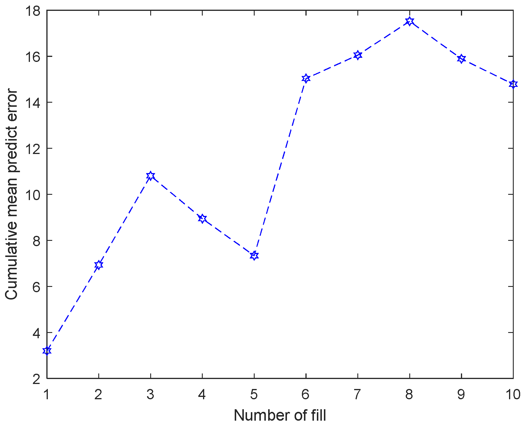
  Calculate the sum of sample errors in the current window;
  Calculate the cumulative average forecast error so far in the current window;
  The difference between the current cumulative average forecast error and the last cumulative average forecast error;
  Judgment drift;
   If drift occurs, the drift monitoring index and LSTM model are updated;
   If no drift occurs, the next sample continues to be predicted using f LSTM Htd ;
   end
  end
end
Predicted value of all samples after all loops is denoted as y ^ Otd .
Table 2. Comparison of prediction performance of different methods.
Detection AlgorithmModel Update TimesUpdate the Required Number of Truth ValuesModel Prediction RMSEMethod
Unsupervised type303026.9249Truth update is required
Supervised type0026.9690Truth detection and updating are required
Textual algorithm101026.9444Using pseudo-truth updates
Table 3. Range of hyperparameter settings.
HyperparameterRadius
Learning rate0.001:0.001:0.03
dropout rate0.1:0.1:0.9
Training times50:5:350
Capacity of error output space detects the drift sample3:1:20
F distribution0.80:0.01:0.99
Contribution rate0.80:0.01:0.99
Disclaimer/Publisher’s Note: The statements, opinions and data contained in all publications are solely those of the individual author(s) and contributor(s) and not of MDPI and/or the editor(s). MDPI and/or the editor(s) disclaim responsibility for any injury to people or property resulting from any ideas, methods, instructions or products referred to in the content.

