Influence Graph-Based Method for Sustainable Energy Systems

Abstract

To reduce carbon emissions from fossil fuel generators in sustainable energy systems, an option is increasing the integration of gas-fired generators into the power system. The increasing reliance on natural gas for electricity generation has strengthened the interdependence between the electric power network and the natural gas infrastructure within the Integrated Power and Gas System (IPGS). This strengthened interdependence increases the risk that disruptions originating in one system may propagate to the other, potentially leading to extensive cascading failures throughout the IPGS. Ensuring the reliability of critical energy infrastructure is vital for sustainable development. This paper proposes a vulnerability assessment method for the IPGS using an influence graph, which can be formulated based on fault chain theory to capture the interactions among failed components in the IPGS. With the influence graph, eigenvector centrality is used to pinpoint the critical components in the IPGS. The proposed methodology is validated using 39-bus 29-node IPGS through the Scenario Analysis Interface for Energy Systems (SAInt) software version 3.5.17.7. Results show that the proposed method has effectively identified the most critical branches in the IPGS, which play a key role in initiating cascading failures. These insights contribute to enhancing the resilience and sustainability of interconnected energy systems.

1. Introduction

The growing electrification of end-use sectors and the increasing reliance on gas-fired power generation have made the integration of power and gas systems essential for operational efficiency and critical for advancing sustainability goals. Integrating natural gas into electric power systems is necessary for meeting growing energy demands and is a promising avenue for enhancing reliability, cost-effectiveness, and environmental sustainability [1]. This integration supports decarbonization by facilitating the integration of renewable energy sources, reducing curtailment, and optimizing the use of low-carbon fuels. By promoting efficient resource allocation and minimizing energy losses during disruptions, IPGS plays a pivotal role in achieving long-term energy sustainability and meeting global climate targets [2]. Multi-energy systems (MESs) further optimize interactions between electricity, heat, transport, and fuels, improving efficiency and performance compared to traditional, isolated energy sectors [3,4].

1.1. Background and Motivation

In an Integrated Power–Gas System (IPGS), energy-coupling components such as gas-fired generators and electricity-driven compressors create complex interactions. From a sustainability perspective, Integrated Power–Gas Systems (IPGSs) contribute to energy efficiency, emission reduction, and resource optimization by enabling flexible load balancing and using cleaner fuel sources. However, these benefits can only be fully realized if the systems remain resilient to disruptions. The complicated interactions between the electricity and natural gas systems impose significant challenges on the reliable operation of the Integrated Electric and Gas System (IEGS), which makes maintaining stable and secure operation more challenging, requiring meticulous and careful management of system dynamics [5,6,7,8]. Due to this interdependence, a failure or disruption triggered in one subsystem could propagate to the other through energy-coupling components and, consequently, affect the operation of various facilities in the IEGS, leading to a catastrophic outage in the entire IPGS [9]. A notable example is the February 2021 U.S Southwest major blackout in Texas following a severe winter storm [10]. It was concluded that the unexpected disconnection of a power line triggered a chain reaction of failures, ultimately resulting in the blackout.

This highlights the critical importance of developing accurate, real-time situational awareness to maintain secure and reliable operation of power systems [GRNN-based real-time fault chain prediction]. Enhancing the reliability and robustness of IPGSs is, therefore, a critical step toward achieving long-term energy sustainability. Therefore, identifying vulnerable components to mitigate potential risk in the IPGS is a critical research challenge.

1.2. State-of-the Art Literature

In this subsection, we provide an overview of the literature most closely related to the scope of this paper. Extensive research has been conducted to evaluate the safety and reliability of Integrated Power–Gas Systems (IPGSs) [11,12]. A study in [13] presented an IPGS model using a Sequential Monte Carlo (SMC) simulation incorporating power-to-gas technologies and gas storage systems to evaluate the system’s reliability. Studies in [14,15] developed a comprehensive model to analyze the impact of interdependencies between electric and natural gas systems on overall system security. The approach incorporated natural gas system constraints into security-constrained power generation to evaluate the vulnerabilities in the electric system. By accounting for stochastic conditions and random failure events, reference [16] proposed a comprehensive mathematical model and flexible simulation tool for the Optimal Energy Flow (OEF) problem applied to an integrated gas generation and transmission system using mixed-integer linear programming (MILP). While these works address reliability at the system level, they generally do not focus on cascading failure propagation or component-level vulnerabilities, especially in the context of interdependencies.

Cascading failures can cause widespread energy disruption and prolonged system downtime, posing a serious threat to sustainability objectives. These failures often begin with unforeseen events, such as equipment malfunctions or natural hazards, and lead to a sequence of interrelated component outages, including transformers and transmission lines [17]. Several research studies have been conducted to identify the critical branches and analyze the vulnerabilities caused by cascading failures to ensure efficient operation. Studies in [18] demonstrate that integrated energy systems are small-world networks, based on the principles of complex network theory, for both weighted and unweighted networks. Therefore, employing complex network theory in integrated systems has been widely used by researchers to evaluate the propagation of cascading failures and their impacts on the entire system. A study on a real interdependent power and gas model using graph theory in [19] concluded that a faulted branch in an integrated system can spread a fault not only to its adjacent branches but also to nonadjacent branches during fault propagation. This concept was also demonstrated in [20], where an integrated steady-state AC power flow model was employed to simulate the propagation of cascading failure within coupled electricity and natural gas systems. These studies reveal that the complex interdependencies between the two networks initiate cascading failures propagating across both systems, underscoring the need for models to go beyond topological proximity.

Because the cascading failure process contains valuable information, such as topological features, power flow distribution, component outage relevance, and system load loss, data-based analysis methods based on historical or simulated cascading failure data have received growing attention recently for analyzing cascading failure propagation. To enhance network robustness and effectively mitigate the impact of intentional disruptions, a topological analysis in [21,22,23] identified the critical branches and investigated the load loss of the electric system. It concluded that electrical networks are highly susceptible to targeted attacks but remain relatively resilient to random failures due to scale-free features. In the context of vulnerability assessment for Power Systems, conventional topological metrics, such as degree, betweenness, and closeness, have been employed to analyze network structures [24]. Extended indices have been introduced to address this limitation and better reflect the behavior of integrated systems under cascading failure scenarios by incorporating electrical parameters into the statistical indices [25]. These modifications enable the construction of weighted and directed network representations. Using these enriched models as the foundation, various network-based metrics [26,27,28,29,30] have been developed to identify critical components to assess system vulnerability accurately. However, these statistical measures fail to capture the physical and operational characteristics inherent to interdependent energy networks.

While the mentioned extended statistical indices incorporate the physical and operational aspects of electrical networks, they primarily emphasize vulnerabilities in electric systems only and often overlook dynamic operational behaviors, particularly in the context of cascading failures within Integrated Power and Gas Systems (IPGSs). As a result, evaluating operative vulnerabilities remains a significant challenge in the IPGS. A promising direction, particularly relevant to IPGSs, is the construction of statistical representations, such as cascading fault graphs currently used in electric systems [31,32,33,34]. Studies in [35,36] quantified the vulnerabilities of electric power systems in cascading fault graphs using indices such as load shedding rate, power flow entropy, residual flow, and continuous temperature changes. The above research indicates that there are indeed critical components and outage relevance in cascading failure, which are the dominating factors in propagation. Since power flow distributions and component connections are changeable in the cascading failure process, the criticalness of components and outage relevance is related to the fault state. Furthermore, the dominating role in propagation should simultaneously consider occurrence frequency and blackout consequences. It combines sequential component outages that may frequently develop into serious faults, resulting in severe blackouts.

1.3. Contribution

To deal with the vulnerability assessment of IPGSs and the dynamic propagation of the cascading failures, this paper proposes a novel approach for vulnerability assessment to identify the vulnerable branches in the IPGS based on influence graphs that characterize the interactions among failed components in the IPGS. Compared to the existing studies, the contribution of this paper is as follows:

• Unified Fault Chain Modeling: Different from previous studies, where the fault chain modeling is only used for the power or gas system separately, we leverage fault chain theory based on the overload mechanism of branches in the IPGS to develop unified fault chain modeling for the entire IPGS, which can further be transformed into an influence graph to characterize the interactions among failed components in the IPGS.
• Dual-Metric Edge Weighting: To characterize the interactions among failed components in the IPGS, unified fault chain modeling is further transformed into an influence graph with dual-metric edge weighting: energy not supplied (ENS) and repetitive failures, which capture the physical and operational aspects of failure propagation in the IPGS.
• Vulnerability Component Identification: With the formulated influence graph, eigenvector centrality is used as a statistical index to identify critical components that not only fail frequently but also significantly impact the ENS in the IPGS. This provides a system-wide view of vulnerability that complements and extends traditional topological and flow-based indices.

These innovations collectively advance the state of the art by offering a system-wide methodology to assess and quantify vulnerability in the IPGS under cascading failure scenarios. The rest of this paper is organized as follows. In Section 2, we characterize cascading failures in the IPGS based on fault chain theory so that an influence graph can be constructed and used to identify vulnerable branches in the IPGS in Section 3. In Section 4, the simulation results are presented to demonstrate the efficacy of the proposed method. The conclusions are drawn in Section 8, in addition to future research.

2. Fault Chain Fundamentals

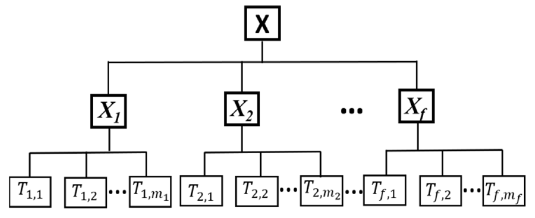
2.1. Fault Chains

Cascading failures are the primary cause of widespread outages and blackouts. The process of contingencies can be described by the fault chain [37,38]. Cascading failures consist of a set of multiple faulted segments or branches that trip one after another in a particular order, as shown in Figure 1, forming a fault chain that eventually leads to an outage. A set of fault chains X in the IPGS can be represented by

$$X=\{X_1,X_2,\dots X_f\}$$

(1)

$$X_i=\{T_{i,j},T_{i,j+1},\dots T_{i,m_i}\}$$

(2)

where X is a set of fault chains of an IPGS network; f is the number of fault chains in the IPGS; m_i is the total number of faulted segments of the fault chain X_i; T_i,j is the jth segment of the fault chain X_i, and j = 1, 2 m_i.

For a fault chain X_i, in the current step j, the next fault event T_i,j+1 depends on the event in the current step T_i,j. This means every next faulted segment is dependent on the current faulted segment. To understand the dependence of the faulted segment in the cascading process of the fault chain X_i, the transition probability is indicated in Equation (3) using the Markov chain [39].

$$P_{xi}\left(T_{i,j}\to T_{i,j+1}\right)=P\left({\displaystyle \frac{P_{i,j+1}}{P_{i,j}}}\right)$$

(3)

The transition probability of all the fault segments in the entire fault chain X_i is expressed as follows:

$$P_{xi}=P\left(T_{i,j}\right)P\left(T_{i,j+1}|T_{i,j}\right)\dots \dots P\left(T_{i,m_i}\right|T_{i,j}.T_{i,j+1}\dots \dots T_{i,m_{i-1} })$$

(4)

It can be summarized as follows:

$$P_{xi}=P\left(T_{i,j}.T_{i,j+1}\dots \dots T_{i,m_i-1 })\right)=P\left({\bigcap }_{j=1}^{m_i}{T}_{i,j}\right)$$

(5)

where P(T_i,j) is the occurrence probability of the first independent random failure of the first fault event T_i,j of the fault chain X_i. P(T_i,j+1|T_i,j) is the transition probability of the second fault event T_i,j+1 of fault chain X_i given that the previous fault event T_i,j has already occurred. It represents that the failure of the segment in fault event T_i,j causes the next segment to fail in T_i,j+1. P(T_i,mi| T_i,j. T_i,j+1…T_i,mi−1) is the probability of the last faulted branch $T_{i,m_i}$ of X_i, given that all the previous faults events T_i,j, T_i,j+1…T_i,mi−1 in the fault chain X_i have occurred and captures the cumulative influence of all previous failure events on the failure probability of T_i,mi.

2.2. Branch Selection in Fault Chains

Based on the transition probability P_xi (T_i,j⟶T_i,j+1) in Equation (3), we can characterize how a fault event propagates in a fault chain. When a fault event T_i,j occurs in the IPGS, this event has different paths to move to the next step, j + 1. The probability of each path is calculated using Equation (5). This probability is related to the overloading of a branch [40] in the IPGS. This paper proposes a branch overloading index to build the fault chain, represented as W:

$$\mathrm{W}={\displaystyle \frac{Z_{fo}-Z_{no}}{Z_{max}}}$$

(6)

where Z_fo is the power flow/gas flow of a branch in the IPGS during a fault; Z_no is the power flow/gas flow of a branch under normal conditions; and Z_max is the maximum power flow/gas flow limit of the branch. Equation (6) shows that if the branch transmits higher power flow/gas flow Z_fo during the fault operation, the value of the overloading index W increases, indicating that the branch is overloaded.

In the IPGS, the power generation and load are constantly changing. To understand the overloading mechanism to generate fault chains, we assume a fault chain X_i is in the j state; for the next state, j + 1, branch A is the candidate branch between the nodes p and q. If the power flow/gas flow P_pq on branch A between bus nodes p and q increases, the failure probability P(A) of branch A will also increase. To calculate the failure probability of branch A and to select it as the next fault segment, the following constraints are considered:

• When the power flow/gas flow P_pq on branch A between the nodes p and q is less than the maximum operation limit of branch A, i.e., when P_pq < P_max, then branch A is not selected as the candidate branch, and its failure probability P(A) = 0.
• When P_pq ≥ 1.3P_max, the failure probability P(A) of branch A is P(A) = 1, and it is selected as the candidate branch showing maximum overload and certain failure.
• When P_max ≤ P_pq < 1.3P_max, the failure probability P(A) of branch A increases linearly, showing overloading but not definite failure. Then, the flow P_pq in branch A is compared to the flow P_pr in the next candidate branch, branch B, between node i and node k. If P_pq > P_pr, then branch A will be selected as the next faulted branch. Otherwise, branch B will be selected as the next fault branch for the event T_i,j+1.

3. Fault Chains for IPGS

3.1. IPGS Modeling

In an IPGS, random initial failures lead to cascading failures with different paths. The cascading depends on which location of the network has the failure initiated. For example, if a line is tripped in the electric network, all the components connected directly or indirectly to that line will be affected, impacting the whole IPGS network. The demand and supply constantly keep on changing until the system reaches stability. Therefore, we need to model the dynamic sequential process of the cascading failures in the IPGS and then implement the procedure of fault chain generation discussed in Section 2.1.

3.1.1. Power Flow Model

In an IPGS, the change in the active and reactive power flow of a bus node i is calculated by

$${\Delta P}_i=P_i-{\sum }_{j=1}^n\left|V_i\right|\left|V_j\right|(G_{ij}\cos \left({\theta }_i-{\theta }_j\right)+B_{ij}\mathrm{s}\mathrm{i}\mathrm{n}\left({\theta }_i-{\theta }_j\right)$$

(7)

$${\Delta Q}_i=Q_i-{\sum }_{j=1}^n\left|V_i\right|\left|V_j\right|G_{ij}\sin \left({\theta }_i-{\theta }_j\right)-B_{ij}\mathrm{c}\mathrm{o}\mathrm{s}\left({\theta }_i-{\theta }_j\right)$$

(8)

where ΔP_i and ΔQ_i denote the power mismatch in the active and reactive power of the bus node i; P_i and Q_i are the active and reactive powers injected into the node i; V_i and V_j are the voltage magnitudes of the node i; θ_i and θ_j are the voltage phase angles between the nodes i and j; and G_ij and B_ij are the real and imaginary parts of the admittance.

During the generation of a fault chain, the total load shedding is determined by AC power flow (ACPF) to measure the degree of power outage. The decision variables for the power system are given by

I = [V   P_G Q_G P_D]

where I is the set of node voltage magnitude V, active and reactive powers of generators P_G and Q_G, and active power demand P_D. The objective function for electric load shedding is given as

$$\min f\left(\mathbf{I}\right)=f\left(P_G\right)-{\sum }_{i=1}^n{\pi }_i{P}_{D,i }$$

(9)

subject to

$${\sum }_{i=1}^n{(P}_{G,i}+P_{Gf,i}+P_{T,i}-P_{F,i}-P_{D,i})=0$$

(10)

$$\left|P_{G,i}^{min}\right|\le \left|P_{G,i}\right|\le \left|P_{G,i}^{max}\right| , i = 1,\dots n$$

(11)

$$\left|Q_{G,i}^{min}\right|\le \left|Q_{G,i}\right|\le \left|Q_{G,i}^{max}\right| , i = 1,\dots n$$

(12)

$$\left|V_i^{min}\right|\le \left|V_i\right|\le \left|V_i^{max}\right| , i = 1,\dots n$$

(13)

$$P_{D,i}^{min}\le P_{D,i}\le P_{D,i}^{set} , i = 1,\dots n$$

(14)

where P_G,i is the power generated by the conventional generator at node i; P_GF,i is the power supply from gas-fired generators to the power system at node i; P_T,i is the power flow entering the node i; P_F,i is the power flow leaving the node i; and n is the total number of nodes in the power system. P_D,i is the load or electric power consumed by electric-driven gas compressors, liquified natural gas (LNG) stations, and power-to-gas (P2G) devices to generate natural gas at node i and must be within the minimum P^min and scheduled load P^set, represented as

$$P_{D,i}={\sum }_{i=1}^n(P_{com,i}+P_{LNG,i}+P_{P2G,i})$$

(15)

The penalty factor π_i reflects the priority of loads and is defined as

$${\pi }_i={max}_{P_{G,x}^{min}\le P_{G,x}\le P_{G,x}^{max}}\left\{\left|{\displaystyle \frac{\partial f\left(P_{G,x}\right)}{\partial P_{G,x}}}\right|\right\}.{\alpha }_{i}x = 1\dots g$$

(16)

where g presents the number of power generators in the IPGS, and α is the prioritizing factor (higher for critical infrastructure loads) of the corresponding load P_D,i [41].

3.1.2. Gas Flow Model

The state variables for gas systems are J = [p G L], where p is the gas pressure; G is the gas flow rate across pipelines; and L is gas demand at nodes. The objective function for gas load shedding is given as

$$\min f\left(\mathbf{J}\right)=f\left(G\right)-{\sum }_{i=1}^m{c}_{0,i}.{\pi }_i{L}_i$$

(17)

subject to

$${\sum }_{i=1}^m{(G}_{s,i}+G_{P2G,i}+G_{in,i}-G_{out,i})=0$$

(18)

$$G_{p,i}=sgn\left(p_i-p_j\right).{\tau }_p.(p_i^2-p_j^2)$$

(19)

$$0\le L_i\le L_i^{max}$$

(20)

$$G_{S,i}^{min}\le G_{S,i}\le G_{S,i}^{max}$$

(21)

$$G_{P2G,i}^{min}\le G_{P2G,i}\le G_{P2G,i}^{max}$$

(22)

$$p_i^{min}\le p_i\le p_i^{max}$$

(23)

where c_o,i is the unit cost coefficient of gas load shedding for gas node i. π_i is the penalty factor for prioritizing load shedding at node i; G_s,i and G_P2G,i represent the gas injected into bus i by gas supply (GS) and P2G. L_i is the gas demand/load at node i and i = 1, 2… m is the total number of nodes in the gas system. G_in,i and G_out,i represent gas flow in/out pipeline p connected to node i; sgn is the sign function indicating flow direction; p_i and p_j represent the pressure at nodes i and j. ${\tau }_p$ is the flow coefficient for pipeline p that depends on the physical parameters (friction factor, diameter, and length) of the pipeline. Equations (21) and (22) define the upper and lower bounds for flows associated with gas pipelines connected to GS and P2G devices. Equation (23) ensures the pressure at each node remains within operational limits. The priority of load shedding is performed using the penalty factor equation, which is

$${\pi }_i={max}_{G_y^{min}\le G_y\le G_y^{max}}\left\{\left|{\displaystyle \frac{\partial f\left(G_y\right)}{\partial G_y}}\right|\right\}.{\alpha }_i$$

(24)

α_i is the prioritizing factor of the corresponding demand L_i and y = 1…g.

When a gas-fired power plant is active, it acts as a gas load to generate active power at coupling node z and is expressed in terms of heat rate efficiency γ_hr (amount of heat (MJ) to generate 1 KWh of power) and gross calorific value, GV, of the fuel [42]. It is expressed as

$$L_{\mathrm{G}\mathrm{f},z}={\displaystyle \frac{{\mathsf{\gamma }}_{hr}.G_{\mathrm{G}\mathrm{f},z}}{GV}}$$

(25)

where z is the coupling node with gas-fired generators connected to it, and z = 1…Gf.

3.1.3. Generator Ramping and Tripping

Failures lead to sudden changes in active power generation and demand. To overcome imbalance or fluctuation between the generation and loads, the generators are modeled for ramping within the upper and lower limit. The maximum and minimum active power generation constraints of a generator i at time step t + 1 are given by

$$P_{G,i}^{max,t+1}=\min \left\{P_{G,i}^{max}.P_{G,i}^t+\omega .∆t\right\}$$

(26)

$$P_{G,i}^{min,t+1}=\max \left\{P_{G,i}^{min}.P_{G,i}^t+\omega .∆t\right\}$$

(27)

where $P_{G,i}^{max,t+1}$ and $P_{G,i}^{min,t+1}$ are the maximum and minimum output limit of generator i at time step t + 1. $P_{G,i}^{max}$ and $P_{G,i}^{min}$ are the absolute maximum and minimum power capacity of generator i under normal conditions. $P_{G,i}^t$ is the power output of generator i at the previous time step t. ω is the maximum MW/min ramp rate of the generator at which it can increase its output. Δt represents the time interval between two consecutive steps. The ramping stops when the generator reaches its maximum or minimum output limit. However, the power and gas supply must be balanced within the given start-up and shut-down time. If the demands are met and there is a surplus output supply, the generators will be tripped in accordance with priority. If there is still an imbalance between supply and demand, load shedding will occur in accordance with the priority levels assigned to each load.

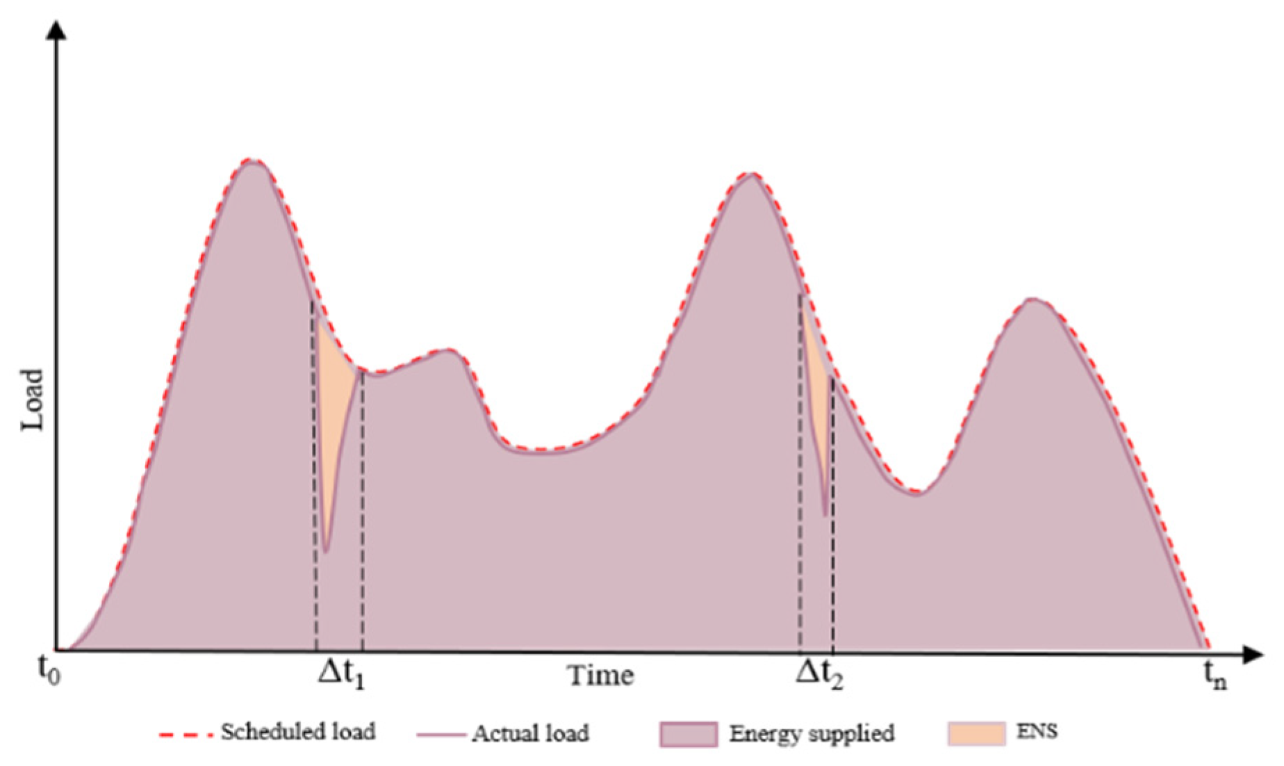
3.1.4. Energy Not Supplied (ENS)

As load shedding is a common consequence of cascading failures in IPGSs, it reflects the severity of these cascading failures, indicating how much energy was not supplied (ENS) due to the failures [43].

In case of failure or disruption, a certain amount of energy may not be served according to demand as scheduled. This could be due to insufficient supply, increased demand, line pack, or limited capacity of transmission lines in the IPGS [44]. In this paper, it is used as an indicator to quantify the impact of disruption on the IPGS network. Figure 2 shows the ENS for the IPGS in case of failure of a network component. The impacts of cascading failure on electricity and natural gas service reliability are evaluated by the two indices of power load shedding and gas load shedding, ENS^power and ENS^gas, caused by a triggering event in the fault chain. Vulnerability indices in the IPGS for the electric and gas ENS ratio are calculated to determine how much of the total load was lost due to cascading failures.

$${ENS}_i^{power}={\displaystyle \frac{\sum _{iϵbus}{(P}_{D,i}^{t_0}-P_{D,i}^{t_n})}{\sum _{iϵbus}{P}_{D,i}^0}}$$

(28)

$${ENS}_e^{gas}={\displaystyle \frac{\sum _{eϵnode}{(L}_e^{t_0}-L_e^{t_n})}{\sum _{eϵnode}{L}_e^0}}$$

(29)

where $P_{D,i}^{t_0}$ and $P_{D,i}^{t_n}$ are the initial and final power loads at node i and $L_e^{t_0}$ and $L_e^{t_n}$ are the initial and final gas loads at node e. The total load loss in the IPGS is calculated by

$$ENS\left(t_n\right)={ENS}_i^{power}\left(t_n\right)+{ENS}_e^{gas}\left(t_n\right)$$

(30)

If ENS = 0, there is no loading shedding, as the system meets all demands, supplying energy as scheduled. ENS = 1 shows complete failure/blackout as the system fails to meet all the load demands. If 0 < ENS < 1, there is partial load shedding, but the system still supplies energy to a few components in the IPGS.

3.2. Construction of Fault Chains Based on IPGS Modeling

By leveraging IPGS modeling, fault chains can be generated via combined dynamic simulation. The procedure for fault chain generation in an IPGS is illustrated as in Figure 3, where to start a combined dynamic simulation, the terminal state of a previous combined steady-state simulation is considered as the initial state. The main steps of this procedure are summarized as follows:

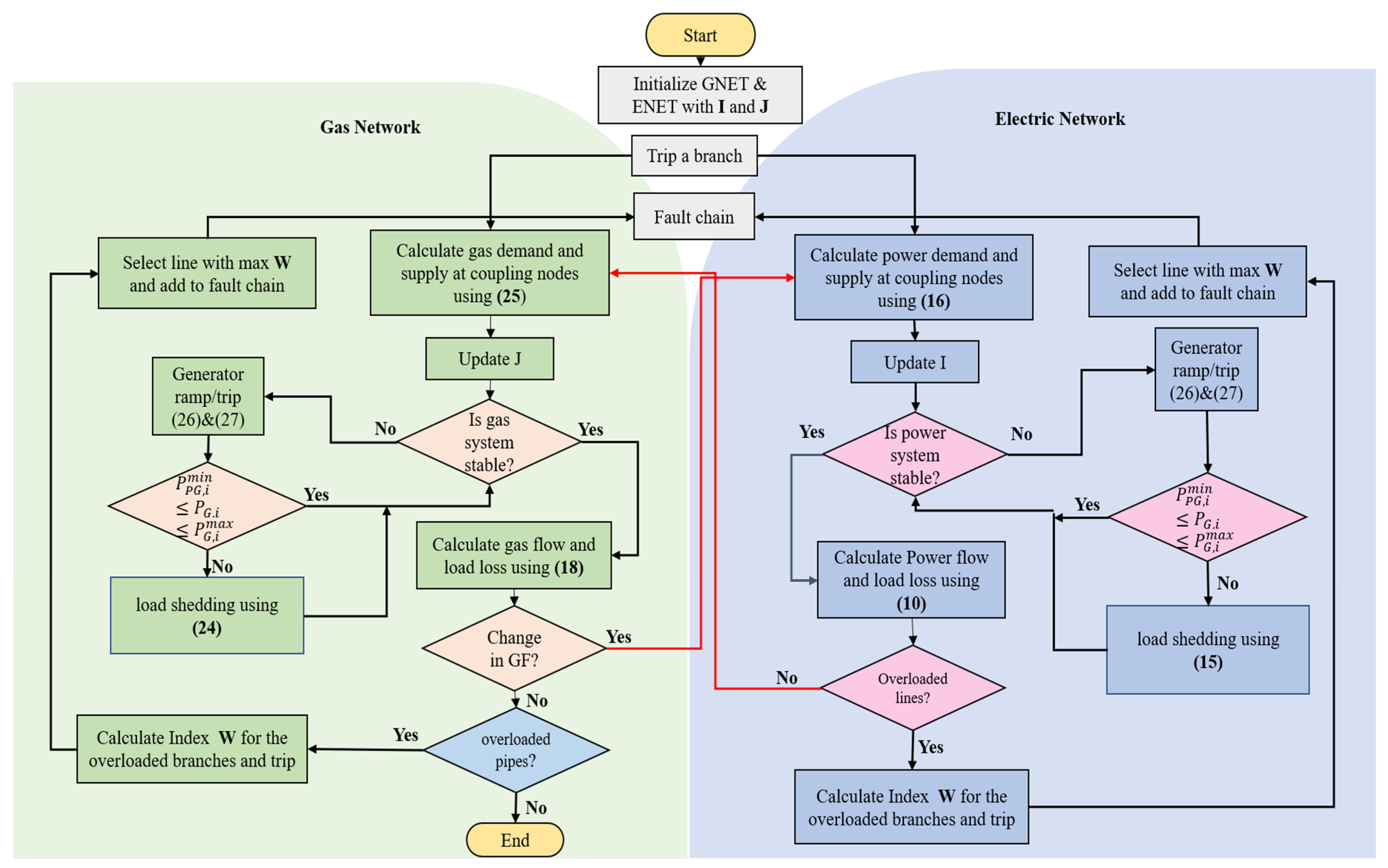
• Initialize the electric network (ENET) and gas network (GNET) with initial state matrix I and J using the terminal state parameters of a previous combined steady-state simulation.
• Select a branch and trip it to initiate the first fault event. Add it to the first fault chain of the fault chain set.
• Calculate the change in demand and supply changes on the coupling nodes using Equations (16) and (25). Update I and J. Calculate the stability of the ENET and GNET using Equations (10) and (18).
• If there is power imbalance, the generators ramp up or ramp down between the maximum and minimum limit set in Equations (26) and (27). The power balance is checked at every step until the ramping of the generators is within the set limits; otherwise, the generator trips and loads are shed in accordance with priority, using Equation (15).
• In case of power flow balance, calculate load losses using Equations (7) and (8) to identify the overloaded lines. The line with the maximum index W in Equation (6) is selected to be added as a faulted segment to the fault chain. In case no overloaded lines exist, go to Step 3. The algorithm calculates the gas supply and demand at the coupling nodes to establish a new gas balance by updating the parameters in J.
• If gas is stable, calculate gas flow using Equation (18) to identify the overloaded lines. The line with the maximum index W in Equation (6) is selected to be added as a faulted segment to the fault chain.
• If there is a gas imbalance, gas generator ramping aids to overcome the imbalance, adhering to the set limits of the generators, or else tripped and prioritized gas load shedding takes place according to Equation (24). The process goes on until gas balance is achieved.
• If the gas network is stable, the gas flow and load losses are calculated using Equations (26) and (27), and the change in gas flow on the coupling nodes is determined. If the gas flow is not the same as calculated in Step 4, repeat Step 3 to analyze a new cascading failure in the power system. Otherwise, go to Step 9.
• In case of no change in the gas flow, check the gas flow limit in each pipeline; the overloaded pipelines are tripped, and the pipelines with the maximum index W are added to the fault chain.
• Calculate load shedding throughout the process using Equation (30). If total load shedding of the IPGS is greater than the set threshold, end the algorithm; otherwise, go to Step 3.

The resulting fault chains are used in Section 3 to construct the influence graph.

4. Influence Graph Construction Based on Fault Chains in IPGS

The influence graph represents the interconnections and dependencies among the faulted components in the IPGS. We take each transmission branch as a starting point to develop fault chains in a given network and then employ the fault chains to construct the influence graph of the network. The nodes represent the branches that include the transmission lines connected to transformers, generators, loads, and other components in the IPGS. The directed edges reflect the propagation path of the fault chain. Using the propagation probabilities of the fault chains from Equation (5), we construct influence graphs based on the change in power/gas flow and the overloading mechanism. The directed and weighted graph represents the temporal characteristics of the generated fault chains.

For a fault chain X_i = {T_i,j, T_i,j+1 … T_i,mi}, the influence graph can be represented by a weighted, directed graph G_i = (V_i, E_i), where Vⁱ = {T_i,j|j = 1, 2, 3…m_i} is the set of nodes, and each node represents a faulted branch; Eⁱ = {E_i,j|j = 1, 2, 3…m_i−1} is the set of edges (or links). The influence graph constructed by f fault chains X₁, X₂,…X_f can be represented as {G = (V,E)|V = V¹ ⋃ V²…⋃ V^f, E¹⋃E²…⋃ E^f}. The weights of the edges are defined by two network metrics that are employed to quantify the vulnerability of the IPGS discussed in the following section.

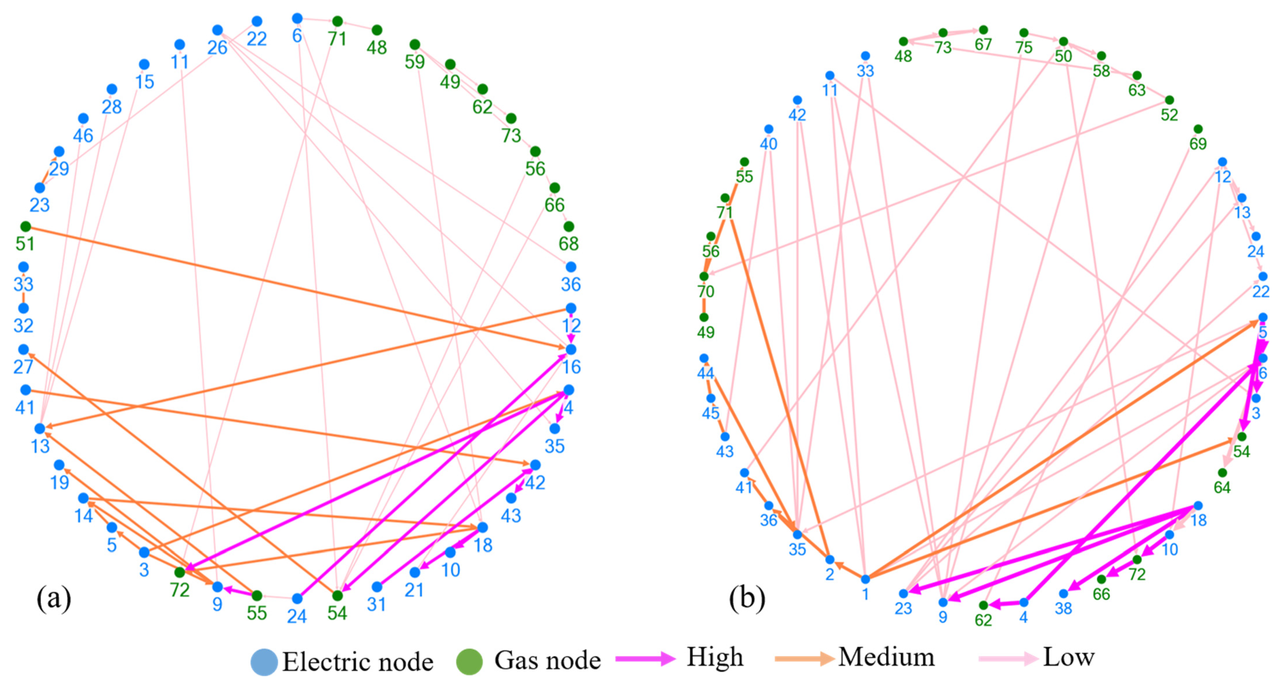
• Edge weight based on ENS: The first vulnerability network metric based on ENS is proposed to measure the impact of cascading failures by quantifying the amount of load that is lost due to system disruptions and how much energy is not supplied due to the failure of components during a cascading failure. A higher load loss leads to a high value of ENS, indicating more power loss and hence greater instability. ENS is calculated for the fault chains and weights of edges, assigned using the following equation:

  $${\delta }_{pq}={\displaystyle \frac{{\delta }_q}{\sum _{j=1}^m{\delta }_{\left(T_{i,j}\right)}}}$$

  (31)

  where δ_pq is the weight of the edge between node p and node q in the graph G; δ_q is the ENS at node q due to the failure of node p; δ(T_i,j) is the total ENS of the fault chain Xi and is calculated using Equation (30).
• Edge weight based on repetitive failures: The second metric evaluates vulnerability based on the repetitive failures of the branches in all the fault chains of the IPGS, which reflects the number of times each branch fails during various random fault scenarios. Components that fail more frequently are considered more vulnerable, as their failure can lead to widespread disruptions in the system. The edge weight between two nodes in the graph G is given by

  $${\beta }_{pq}={\displaystyle \frac{n_p}{\sum _{k=1}^f{n}_k}}$$

  (32)

  where β_pq represents the weight between the nodes p and q, n_p is the number of times the branch p occurs in all fault chains; and f is the total number of fault chains in the IPGS. The weight of the edges shows the statistical association of vulnerability among the affected nodes in the influence graph. Together, these two metrics offer a comprehensive assessment to quantify the vulnerability of the system by considering both the consequences of failure and the reliability of individual components.

To illustrate this influence graph, a simple example of a six-bus IPGS is shown in Figure 4. The power system is integrated into the gas system through a P2G device at the coupling nodes. Buses 1 and 6 are load buses in the gas system, and buses 1 and 2 are generator buses. The power system shows buses 4 and 5 as load buses and buses 4 and 5 as generator buses. The IPGS has a set of three fault chains X = {X₁, X₂, X₃}, as shown in

Table 1. Set of fault chains in 6-bus system.

Fault Chains	Ti, j	Ti, j+1	Ti, j+2	Ti, j+3
X1 = {b1, b2, b6}	b1	b2	b6
X2 = {b2, b6, b4}	b2	b6	b4
X3 = {b3, b1, b2, b5}	b3	b1	b2	b5

. With the set of fault chains, the graph in Figure 5 is constructed through the following steps to characterize the propagation of all faulted events in the IPGS based on repetitive failure.

• For the fault chain X₁, we first create a directed graph H₁ with three nodes, as shown in Figure 5a, where nodes represent faulted branches b1, b2, and b6 in the six-node IPGS. The directed edge from b1 to b2 represents the fault propagating from branch b1 to branch b2 in X₁, and the directed edge from b2 to b6 represents the fault further spreading from branch b2 to b6 in X₁.
• For the fault chain X₂, the directed graph H₁ will be extended to graph H₂ by adding additional node b4 to graph H₁ as shown in Figure 5b. Similarly, to the nodes and edges in graph H1, additional b4 nodes represent a faulted branch in the six-bus IPGS, and the directed edges among these nodes represent the fault propagating from branch b6 to b4 in X₂.
• Graph G in Figure 5c is generated by repeating step 2 to include the fault branches in fault chain X₃.

The branch b2 appears to be faulted in all three fault chains, X₁, X₂, and X₃, and the propagation of faults from b1 to b2 appears twice. Therefore, node b2 is highly vulnerable to failure in all the fault chains, and the path of failure propagation from branch b1 to branch b2 shows that the transition probability of a fault to propagate from branch b1 to branch b2 is higher than a fault propagating from branch b1 to any other branch in the IPGS.

5. Identification of Critical Branches in the IPGS Based on Influence Graph

In IPGSs, failures exhibit strong interdependencies; even small disturbances can cascade through critical corridors, regardless of local connectivity. Failures typically originate from important nodes that are connected to other influential nodes, rather than from highly connected but less significant ones. Eigenvector centrality provides a multidimensional perspective by quantifying the global importance of a node based on its connections to other influential nodes. It is used to identify the nodes that could act as indirect bridges towards failure propagation [45]. Unlike degree centrality, which simply counts connections, or betweenness centrality, which focuses on shortest paths, eigenvector centrality captures how faults propagate preferentially through critical hubs rather than along minimal routes [46]. A node with high eigenvector centrality is often connected to the influential nodes that themselves have high-degree centrality. In the IPGS, nodes with high eigenvector scores play pivotal roles in maintaining the stability of the network and, in case of disruptions, may lead to widespread failure due to connections with other critical components. By identifying these critical nodes and potential vulnerable paths, it gives insight into making targeted strategies to mitigate cascading failures and bolster network resilience.

For graph G with V nodes, let A = (A_pq) if node p is linked to node q; then, the adjacency matrix A_pq = 1. Then, the eigenvector centrality x_p of a node p with a set N of neighboring nodes is given by

$$x_p={\displaystyle \frac{1}{\lambda }}{\sum }_{q\in N\left(p\right)}{\mathit{A}}_{pq}{x}_q$$

(33)

where A_pq is the adjacency matrix of graph G, representing the edge weight from node p to node q. N(p) is the set of nodes that are directly influenced by node p (i.e., nodes with directed edges from node p to q); λ is the scaling factor; and x_q is eigenvector centrality of node q. Initially, every node has the same score considering a neutral starting point. Over successive iterations, the centrality score for every node is updated depending on its connections with the influential neighbor nodes. This process continues until the algorithm is converged, giving final eigenvector centrality scores for all the nodes.

To use the use eigenvector centrality in influence graph G based on ENS, if there is a directed edge from node p to node q, (p→q), and the transition probability of failure to propagate from node p to node q is P_δ(p→q), then the adjacency matrix A is populated with weight δ_pq using Equation (31), given by

$${\mathit{A}}_{pq}=P_{\delta }\left(p\to q\right).{\delta }_{pq}$$

(34)

Equation (33) is used to calculate the eigenvector centrality for node p:

$$x_p={\displaystyle \frac{1}{\lambda }}{\sum }_{q\in N\left(p\right)}{P}_{\delta }\left(p\to q\right).{\delta }_{pq}.x_q$$

(35)

Similarly, to use eigenvector centrality in influence graph G based on repetitive failures, if there is a directed edge from node p to node q (p→q), and the transition probability of failure to propagate from node p to node q is P_β(p→q), then the adjacency matrix A is populated with weight β_pq using Equation (31), given by

$${\mathit{A}}_{pq}=P_{\beta }\left(p\to q\right).{\beta }_{pq}$$

(36)

Equation (33) is used to calculate the eigenvector centrality for node p:

$$x_p={\displaystyle \frac{1}{\lambda }}{\sum }_{q\in N\left(p\right)}{P}_{\beta }\left(p\to q\right).{\beta }_{pq}.x_q$$

(37)

To ensure that centrality values sum to 1 and can be interpreted as influence, x is normalized.

6. Results

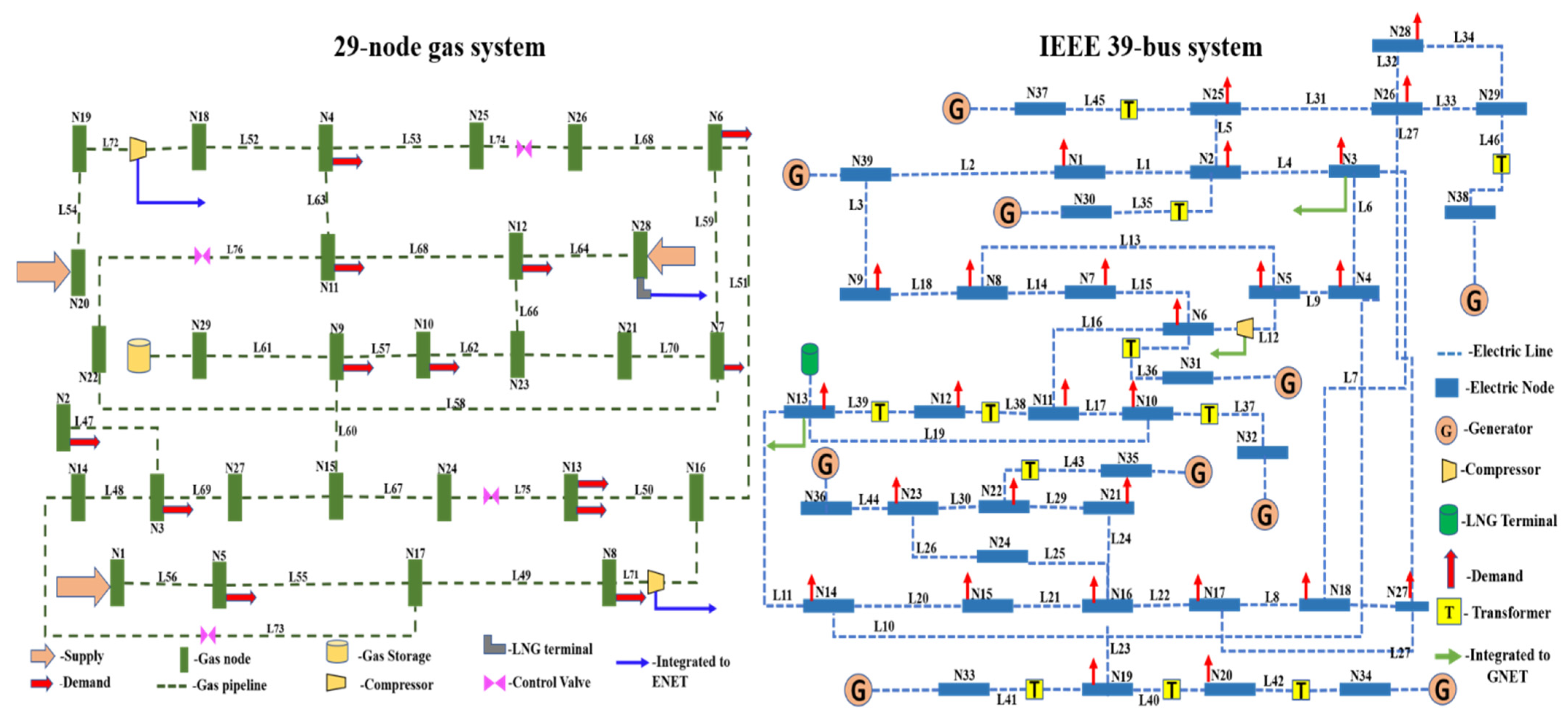
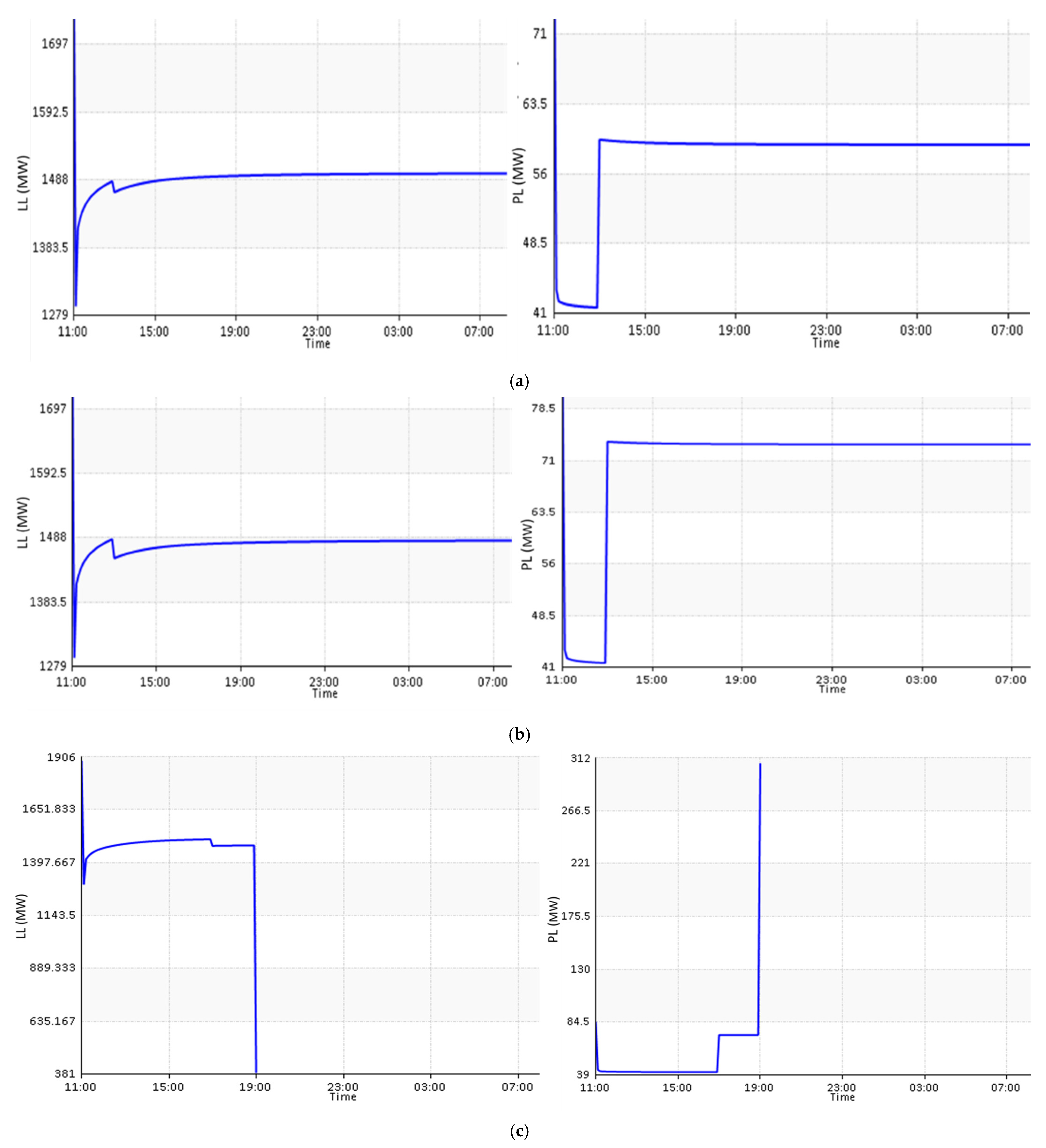
6.1. 39-Bus 29-Node IPGS

To demonstrate the efficacy of the proposed methodology, a 39-bus 29-node IPGS is modeled as shown in Figure 6, which includes 68 nodes, 78 branches, 13 generators, 42 demands, an electric-driven gas compressor, an electric-driven LNG, and a P2G device on the cEncoordoupling nodes. The Scenario Analysis Interface for Energy Systems (SAInt), an integrated system modeling platform provided by Encoord Inc., is employed as a co-simulation tool using different base scenarios with several events under different operating conditions. Each scenario considers a fault occurring in one transmission line or pipeline at a time. This time-series data from the base scenarios is augmented using a synthetic data generation technique to generate cascading failures, considering the fault occurring on one, two, or three transmission lines or gas pipelines.

Fault chain sets are obtained by the method in Section 2 based on transition probabilities from Equation (5).

Table 2. Fault chains in 39-bus 29-node IPGS.

Branch	Fault Chains	Branch	Fault Chains
1	1-3-(5,9),9-(11,14,18,19,20)	18	18-(7,8,9,13),13-(14,15,16,20),20-(21,22,27,31)
2	2-3-(5,9), 9-(11,12,13,14), 14-(18,20)	4,18	4-(1,5,6,54,55,35),17-(3,12,14)
24	24-(25,26,30)	53,55	53-(54,55,4,6,7)
15	15-(27,29),29-31	67	67-(57,39,19)
1,17	1-3-(5,9),9-(11,14,18,19,20,59,64),16-(37,38)	11,13	11-(9,12,15,16,67), 16-(21,22),3-(1,2,4,6,13)

shows a few fault chains formed due to random failure events occurring in one and two lines/pipelines. It is observed that interactions in the power system are denser than that in the gas system. This is because, in case of disruption or failure, the electric system reaches a new operational state instantaneously, as electricity travels at the speed of light. On the other hand, the transportation velocity of natural gas in the gas system is very low, typically 10 m/s [47]. Any disturbance in the gas system leads to slow transient behavior before reaching a new stable operation state. To this end, co-simulation of a quasi-dynamic ACPF power system and a dynamic gas flow model is considered.

However, it can also be noted that the fault that triggers to and from the gas network affects the IPGS due to interdependency via a hub. Unlike previous studies, this paper reveals the relationship between the critical lines, considering the electric network and the gas network as one system, and then analyzes fault propagation using vulnerability indices to quantify the vulnerability of the IPGS.

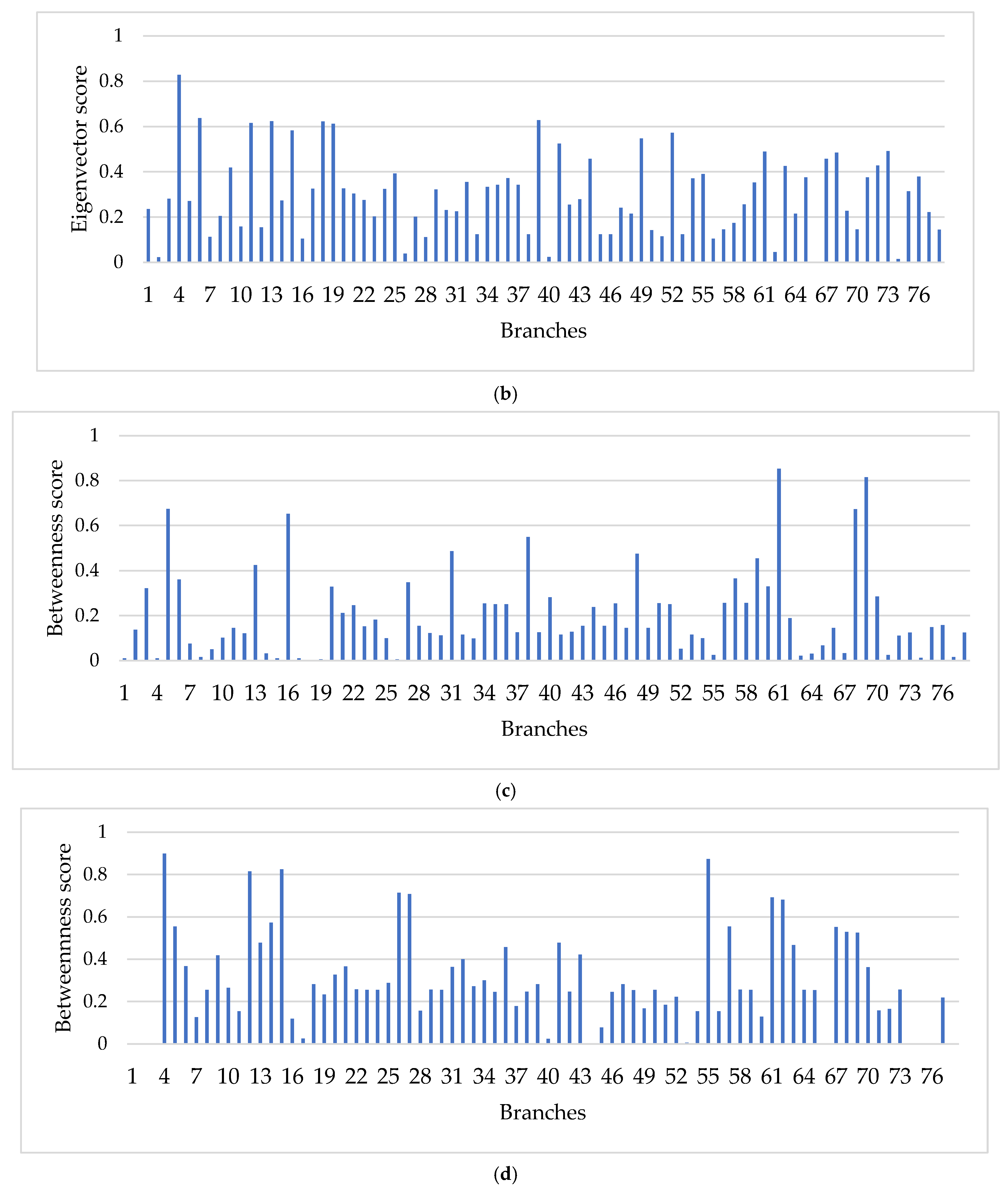
6.2. Influence Graph Analysis for IPGS

To generate the influence graph for the IPGS model, the nodes in the fault chain with weighted edges are used. The nodes represent faulted branches in the IPGS, such as electric lines or gas pipelines, that are connected to other substations and components susceptible to faults, which play a crucial role in the propagation of failures in the IPGS. The directed edges between nodes represent the potential path of cascading failures that propagate to the next node. Each edge is assigned a weight that quantifies the ENS during the failure, resulting in potential load loss and the repetitive failure of branches if a fault propagates along this path. The higher the weights, the higher the impact severity of failure on the IPGS. To reveal the vulnerability of the IPGS, influence relationships between the nodes are divided into three categories, with edges illustrated in three colors, indicating high-, medium-, and low-vulnerability relations among faulted branches.

Figure 7 shows the influence graph highlighting high-, medium-, and low-vulnerability interactions among the faulted lines based on ENS and repetitive failures. These interactions contribute to both load loss and power loss in the IPGS.

Table 3. Total load loss and power loss in IPGS due to highly vulnerable paths based on ENS.

Case	Adjacent Relations	Total Load Loss MW	Total Power Loss MW
1	4-(35,54,72)	1533.91	84.831
2	18-(10,21)	1485.99	76.221
3	(12,24)-16	1512.76	49.447
4	31-(42,43)	1498.73	63.537

and

Table 4. Total load loss and power loss in IPGS due to highly vulnerable paths based on repetitive failures.

Case	Adjacent Relations	Total Load Loss MW	Total Power Loss MW
1	5-(3,6,54)	1467.677	111.102
2	18-(3,38,23)	1522.179	40.057
3	10-72-66	1531.569	42.283

summarize the total load loss and power loss in IPGS due to highly vulnerable paths identified through ENS and repetitive failure metrics.

To validate the results for the highly vulnerable interactions, four test cases are simulated based on ENS, and four additional test cases are conducted based on repetitive failure to observe the system’s response, as shown in Figure 8 and Figure 9.

In case 1, the failure that propagates from electric line 4 to electric branch 35 and gas branches 54 and 72 shows higher load loss and a high value of power loss in the IPGS, as shown in Table 3. This is because when a disruption occurs in a gas system, such as pipeline failure or gas compressor malfunction, it takes time for the system to respond, as shown in Figure 8. During this period, gas supply to gas-fired power plants at the coupling nodes is reduced or cut off, leading to the loss of generation in the power system, which increases load loss. Although the response of the gas system shows a decrease in line pack, there is an increase in flow balance due to the redistribution of gas and power flow in the IPGS.

Similarly, for cases 2, 3, and 4, the influence relations in the graph characterize the vulnerability of the critical branches that contribute to the maximum load loss and power loss in the IPGS. The highly vulnerable branches in case 2 and case 3 lead to high load loss and power loss, but in this case, the line pack acts as a buffer to supply gas for a short period of time, maintaining gas flow and flow balance, as illustrated in Figure 8.

In case 3, electric branch 31 leads branch 42 and 43 in the power system to fail. These two branches are directly connected to transformers, as shown in Figure 6. The failure of these branches leads to overloading of the neighboring branches, causing generator outages and imbalance in the supply and demand, hence reducing the gas supply at the coupling nodes. The drop in the line pack is shown in Figure 8.

Based on repetitive failures, case 1 exhibits the highest power loss in the IPGS, illustrated in Table 4. Failure at branch 5 causes 3, 6, and 54 to fail, indicating the failure of supply, an electric-driven gas compressor, and the loads connected to them. The line pack graph in Figure 9 shows a gradual decrease in gas flow, causing an increase towards flow balance. Cases 2 and 3 also show a similar trend, with a decrease in line pack, which indicates a decrease in gas flow, but at the same time, the system shows an increase in flow balance to maintain stability.

The two influence graphs show different influence relations among the faulted branches based on the vulnerability indices. This ensures analysis of the vulnerability of IPGS from different aspects. The transition probability of the vulnerable branches for all cases is calculated using Equation (5), where highly vulnerable branches show a transition probability of ≤2.52 × 10⁻², and the transition probability for medium and low vulnerable branches is ≤3.03 × 10⁻² and ≤3.07 × 10⁻². The highly vulnerable branches show a lower transition probability, indicating that these branches are less likely to fail in random failures, but once they fail, it triggers cascading failures in the IPGS, leading to maximum load loss and power loss.

6.3. Identification of Critical Branches

To pinpoint the most critical nodes among all the highly vulnerable branches, eigenvector centrality is employed alongside betweenness centrality for comparative analysis. The graphs in Figure 10a,b illustrate the eigenvector centrality score for the IPGS network based on the network indices, while Figure 10c,d show the corresponding betweenness centrality scores.

To further validate the results, the identified highly vulnerable lines are deliberately tripped individually and then sequentially. In Figure 11a,b below, the load loss and power loss in the IPGS are shown when line 4 is tripped. It is observed that when line 4 is tripped alone, load loss increases in the IPGS, and so does power loss, and continues to stay in the same state until power flow is redistributed. A similar trend is observed when line 18 is tripped.

However, it is observed that despite the increase in load loss and power loss, the IPGS does not shut down. In Figure 11c, when lines 4 and 18 are tripped together, load loss decreases, but at the same time, due to a sudden increase in power loss, the IPGS shuts down, indicating an outage.

This process was repeated multiple times under varying operating conditions for the identified vulnerable branches. While the eigenvector and betweenness centrality scores fluctuated across cases, branches 4 and 18 consistently exhibited the highest eigenvector scores, while branch 4 maintained the highest betweenness score, indicating these as the highest vulnerable branches. Results conclude that tripping the critical lines individually leads to a high load loss and power loss in the IPGS, but tripping them simultaneously or sequentially results in a blackout.

Therefore, from the results, it can be reasoned that using one vulnerability index alone does eliminate the risk of cascading failures that lead to large-scale blackouts. If more than one vulnerability index is employed, it improves the identification of vulnerable components. The analysis also proved that using eigenvector centrality along the vulnerability indices aids in understanding the criticality of the nodes and mitigating the potential risks.

7. Discussion

7.1. Discussion on Influence Graph Analysis for IPGS Based on ENS and Repititive Failures

The influence graph in Figure 7a shows the high-, medium-, and low-vulnerability interactions among faulted lines based on ENS. The four interactions 4-(35,54,72), 18-(10,21), (12,24)-16, and 31-42-43 show the branches that contribute to a high value of ENS. This means that if a branch fails, leading to a certain amount of ENS in the IPGS, it will cause more lines to fail due to an insufficient supply of energy. As we focus on identifying the most critical branches in the IPGS, we only consider the cases for highly vulnerable interactions. It can be observed from the influence graph that two branches, 54 and 72, in the gas system are affected due to branch 4 in the electric system. These lines are connected to the coupling components, as shown in Figure 6, hence characterizing the interdependencies of both systems in the IPGS. The graph also reveals that only three branches of the gas system contribute to the propagation path of high vulnerability. Table 3 shows the total load loss and power loss in the IPGS caused due to failure of branches in the highly vulnerable paths.

7.2. Discussion on Identification of Critical Branches Using Eigenvector Centrality

As illustrated in Figure 10a, only one branch, i.e., branch 18, out of 78 branches exhibits the highest eigenvector centrality score of 0.6201 based on ENS. This means that branch 18 is a critical branch, as it is connected to highly influential branches, and in the case of failure, it would fail the other critical components in the IPGS, leading to widespread outage. Five out of seventy-seven branches have eigenvector scores greater than 0.5, which shows that, in case of failure, these branches will contribute to fault propagation in the IPGS but will not lead to higher load loss power losses than branch 18. The remaining 72 branches have eigenvectors scores of less than 0.5, indicating that, in case of failure, they would not cause significant damage to the IPGS.

As shown in Figure 10b, branch 4 has the highest eigenvector centrality based on repetitive failures in the case of multiple cascading failures. This means that branch 4 is highly vulnerable and is likely to fail in all random cascading failures in the IPGS. The two analyses of eigenvector centrality reveal that nodes 4 and 18 are highly vulnerable branches, which means that disruptions in these branches will not only directly affect operations in the IPGS but will also indirectly affect power flow, leading to blackouts. It also indicates that these branches are the most critical ones among all the identified vulnerable branches, as they are connected to the high-impact nodes in the IPGS.

As illustrated in Figure 10c,d, branch 61 and 69 exhibit the highest betweenness centrality score, indicating that they frequently lie on the shortest and most critical fault propagation paths associated with ENS. Furthermore, under repetitive failure-based analysis, branches 4, 15, and 55 show notably high betweenness centrality scores, revealing their significance in multiple cascading failure sequences. Since betweenness centrality reflects how often a branch lies along the shortest paths between different node pairs, the high scores for branches 4, 15, 55, 61, and 69 indicate their key role in cascading propagation, making them critical components within the IPGS.

7.3. Performance of Proposed Method

To evaluate the effectiveness of the proposed approach, it is compared against the conventional centrality-based method, which identifies critical components using an interaction graph constructed from same network metrics, followed by betweenness centrality analysis. Using betweenness centrality, five out of seventy-eight branches (6.4%) in the IEEE 39-bus 29-node IPGS were identified as critical. However, only one of these five branches were was associated with a severe load loss event resulting in a blackout, indicating that some non-critical lines may have been misclassified. In contrast, the proposed method identified only two branches out of seventy-eight (2.6%) as critical, both of which were validated to be highly influential causing a complete blackout when tripped together. This validates that the proposed method outperforms the baseline approach, demonstrating its ability to detect the highly critical and vulnerable components in the Integrated Power and Gas System (IPGS).

Given its demonstrated performance, the proposed influence graph-based vulnerability assessment method offers significant potential for practical applications in both the operation and planning of integrated energy systems. The proposed influence graph-based vulnerability assessment method has broad applicability in the operation and planning of integrated energy systems. It can support system planners in identifying and prioritizing critical components that pose the highest risk for cascading failures, enabling proactive maintenance and targeted upgrades. Additionally, this approach can be integrated into contingency analysis tools to support decision-making for system planning. Beyond reliability assessment, it also has value in informing resilience planning and policy development aimed at strengthening the security and sustainability of multi-energy systems.

8. Conclusions and Future Work

In this paper, a novel influence-based analysis was proposed to assess the vulnerability of IPGSs. In this method, an influence graph was constructed based on fault chain theory, along with ENS and repetitive failures as edge weights, to characterize the interaction among faulty components in the IPGS. With the influence graph, eigenvector centrality was used to pinpoint the critical branches, whose failures could initiate cascading failures in the IPGS. The proposed method was validated on a 39-bus 29-node IPGS model. The proposed method can be used to identify vulnerable components to prevent and mitigate failures in the IPGS to improve its reliability. Implementing early failure detection can prevent widespread outages. In future research, we will enhance the proposed method by integrating real-time operational data to improve the overall reliability of Integrated Power–Gas Systems (IPGSs). To this end, we plan to explore advanced machine learning approaches, particularly deep learning and graph neural networks (GNNs), which are well-suited for capturing the nonlinear and evolving relationships present in complex, large-scale networks. By leveraging historical and real-time system data, these models can provide early warning signs of potential failures, allowing preventive actions before disruptions spread. Incorporating such data-driven techniques will enable more responsive and informed operational decisions and contribute to designing intelligent monitoring frameworks that can significantly improve the resilience and stability of IPGS operations.

References

1. Zhou, Y.; He, C. A Review on Reliability of Integrated Electricity-Gas System. Energies 2022, 15, 6815. [Google Scholar] [CrossRef]
2. Khatibi, M.; Rabiee, A.; Bagheri, A. Integrated Electricity and Gas Systems Planning: New Opportunities, and a Detailed Assessment of Relevant Issues. Sustainability 2023, 15, 6602. [Google Scholar] [CrossRef]
3. Agarwal, A.; Sharma, T. Integrated energy system modeling perspectives for future decarbonization pathways based on sector coupling, life-cycle emissions and vehicle-to-grid integration. Renew. Sustain. Energy Rev. 2025, 215, 115620. [Google Scholar] [CrossRef]
4. Li, J.; Liu, J.; Yan, P.; Li, X.; Zhou, G.; Yu, D. Operation Optimization of Integrated Energy System under a Renewable Energy Dominated Future Scene Considering Both Independence and Benefit: A Review. Energies 2021, 14, 1103. [Google Scholar] [CrossRef]
5. Wang, Y.; Yang, Y.; Xu, Q. Integrated planning of power-gas systems considering N-1 constraint. Energy Rep. 2023, 9, 1274–1281. [Google Scholar] [CrossRef]
6. Correa-Posada, C.; Sánchez-Martín, P. Integrated Power and Natural Gas Model for Energy Adequacy in Short-Term Operation. IEEE Trans. Power Syst. 2015, 30, 3347–3355. [Google Scholar] [CrossRef]
7. Shahidehpour, M.; Fu, Y.; Wiedman, T. Impact of natural gas infrastructure on electric power systems. Proc. IEEE 2005, 93, 1042–1056. [Google Scholar] [CrossRef]
8. Portante, E.; Kavicky, J.; Craig, B.; Talaber, L.; Folga, S. Modeling Electric Power and Natural Gas System Interdependencies. J. Infrastruct. Syst. 2017, 23. [Google Scholar] [CrossRef]
9. Wang, Y.; Yang, Y.; Xu, Q. Reliability Assessment for Integrated Power-gas Systems Considering Renewable Energy Uncertainty and Cascading Effects. CSEE J. Power Energy Syst. 2023, 9, 1214–1226. [Google Scholar] [CrossRef]
10. Shrestha, S.; Panchalogaranjan, V.; Moses, P. The February 2021 US Southwest power crisis. Electr. Power Syst. Res. 2023, 217, 109124. [Google Scholar] [CrossRef]
11. Chen, S.; Conejo, A.; Sioshansi, R.; Wei, Z. Equilibria in Electricity and Natural Gas Markets with Strategic Offers and Bids. IEEE Trans. Power Syst. 2020, 35, 1956–1966. [Google Scholar] [CrossRef]
12. Koltsaklis, N.; Dagoumas, A. State-of-the-art generation expansion planning: A review. Appl. Energy 2018, 230, 563–589. [Google Scholar] [CrossRef]
13. Zeng, Z.; Ding, T.; Xu, Y.; Yang, Y.; Dong, Z. Reliability Evaluation for Integrated Power-Gas Systems with Power-to-Gas and Gas Storages. IEEE Trans. Power Syst. 2020, 35, 571–583. [Google Scholar] [CrossRef]
14. Xie, H.; Sun, X.; Chen, C.; Bie, Z.; Catalao, J. Resilience Metrics for Integrated Power and Natural Gas Systems. IEEE Trans. Smart Grid 2022, 13, 2483–2486. [Google Scholar] [CrossRef]
15. Duan, J.; Liu, F.; Yang, Y.; Jin, Z. Flexible Dispatch for Integrated Power and Gas Systems Considering Power-to-Gas and Demand Response. Energies 2021, 14, 5554. [Google Scholar] [CrossRef]
16. Tan, Y.; Wang, X.; Zheng, Y. A new modeling and solution method for optimal energy flow in electricity-gas integrated energy system. Int. J. Energy Res. 2019, 43, 4322–4343. [Google Scholar] [CrossRef]
17. Zhao, Y.; Cai, B.; Cozzani, V.; Liu, Y. Failure dependence and cascading failures: A literature review and research opportunities. Reliab. Eng. Syst. Saf. 2025, 256, 110766. [Google Scholar] [CrossRef]
18. Qin, C.; Wang, L.; Han, Z.; Zhao, J.; Liu, Q. Weighted directed graph based matrix modeling of integrated energy systems. Energy 2021, 214, 118886. [Google Scholar] [CrossRef]
19. Beyza, J.; Correa-Henao, G.J.; Yusta, J.M. Cascading Failures in Coupled Gas and Electricity Transmission Systems. In Proceedings of the 2018 IEEE Andescon, Santiago de Cali, Colombia, 22–24 August 2018. [Google Scholar]
20. Bao, Z.; Jiang, Z.; Wu, L. Evaluation of bi-directional cascading failure propagation in integrated electricity-natural gas system. Int. J. Electr. Power Energy Syst. 2020, 121, 106045. [Google Scholar] [CrossRef]
21. Xie, B.; Li, C.; Wu, Z.; Chen, W. Topological Modeling Research on the Functional Vulnerability of Power Grid under Extreme Weather. Energies 2021, 14, 5183. [Google Scholar] [CrossRef]
22. Panigrahi, P.; Maity, S. Structural vulnerability analysis in small-world power grid networks based on weighted topological model. Int. Trans. Electr. Energy Syst. 2020, 30, 12401. [Google Scholar] [CrossRef]
23. Xie, B.; Tian, X.; Kong, L.; Chen, W. The Vulnerability of the Power Grid Structure: A System Analysis Based on Complex Network Theory. Sensors 2021, 21, 7097. [Google Scholar] [CrossRef] [PubMed]
24. Zhang, Y.; Kang, Z.; Guo, X.; Lu, Z. The Structural Vulnerability Analysis of Power Grids Based on Overall Information Centrality. IEICE Trans. Inf. Syst. 2016, E99D, 769–772. [Google Scholar] [CrossRef]
25. Chopade, P.; Bikdash, M. New centrality measures for assessing smart grid vulnerabilities and predicting brownouts and blackouts. Int. J. Crit. Infrastruct. Prot. 2016, 12, 29–45. [Google Scholar] [CrossRef]
26. Liu, B.; Li, Z.; Chen, X.; Huang, Y.; Liu, X. Recognition and Vulnerability Analysis of Key Nodes in Power Grid Based on Complex Network Centrality. IEEE Trans. Circuits Syst. II-Express Briefs 2018, 65, 346–350. [Google Scholar] [CrossRef]
27. Kang, Z.; Zhang, Y.; Guo, X.; Lu, Z. The Structural Vulnerability Analysis of Power Grids Based on Second-Order Centrality. IEICE Trans. Fundam. Electron. Commun. Comput. Sci. 2017, E100A, 1567–1570. [Google Scholar] [CrossRef]
28. Forsberg, S.; Thomas, K.; Bergkvist, M. Power grid vulnerability analysis using complex network theory: A topological study of the Nordic transmission grid. Phys. A-Stat. Mech. Its Appl. 2023, 626, 129072. [Google Scholar] [CrossRef]
29. Bose, D.; Chanda, C.; Chakrabarti, A. Vulnerability assessment of a power transmission network employing complex network theory in a resilience framework. Microsyst. Technol.-Micro-Nanosyst.-Inf. Storage Process. Syst. 2020, 26, 2443–2451. [Google Scholar] [CrossRef]
30. Espejo, R.; Lumbreras, S.; Ramos, A. Analysis of transmission-power-grid topology and scalability, the European case study. Phys. A-Stat. Mech. Its Appl. 2018, 509, 383–395. [Google Scholar] [CrossRef]
31. Ju, W.; Sun, K.; Qi, J. Multi-Layer Interaction Graph for Analysis and Mitigation of Cascading Outages. IEEE J. Emerg. Sel. Top. Circuits Syst. 2017, 7, 239–249. [Google Scholar] [CrossRef]
32. Zhu, Y.; Yan, J.; Tang, Y.; Sun, Y.; He, H. Resilience Analysis of Power Grids Under the Sequential Attack. IEEE Trans. Inf. Forensics Secur. 2014, 9, 2340–2354. [Google Scholar] [CrossRef]
33. Wei, X.; Gao, S.; Huang, T.; Bompard, E.; Pi, R.; Wang, T. Complex Network-Based Cascading Faults Graph for the Analysis of Transmission Network Vulnerability. IEEE Trans. Ind. Inform. 2019, 15, 1265–1276. [Google Scholar] [CrossRef]
34. Zang, T.; Gao, S.; Huang, T.; Wei, X.; Wang, T. Complex Network-Based Transmission Network Vulnerability Assessment Using Adjacent Graphs. IEEE Syst. J. 2020, 14, 572–581. [Google Scholar] [CrossRef]
35. Fang, R.; Shang, R.; Wang, Y.; Guo, X. Identification of vulnerable lines in power grids with wind power integration based on a weighted entropy analysis method. Int. J. Hydrogen Energy 2017, 42, 20269–20276. [Google Scholar] [CrossRef]
36. Yang, S.; Chen, W.; Zhang, X.; Liang, C.; Wang, H.; Cui, W. A Graph-Based Model for Transmission Network Vulnerability Analysis. IEEE Syst. J. 2020, 14, 1447–1456. [Google Scholar] [CrossRef]
37. Guo, Z.; Sun, K.; Su, X.; Simunovic, S. A review on simulation models of cascading failures in power systems. Ienergy 2023, 2, 284–296. [Google Scholar] [CrossRef]
38. Zakariya, M.; Teh, J. A Systematic Review on Cascading Failures Models in Renewable Power Systems with Dynamics Perspective and Protections Modeling. Electr. Power Syst. Res. 2023, 214, 108928. [Google Scholar] [CrossRef]
39. Zhai, C.; Nguyen, H.; Xiao, G. A robust optimization approach for protecting power systems against cascading blackouts. Electr. Power Syst. Res. 2020, 189, 106794. [Google Scholar] [CrossRef]
40. Wei, X.; Zhao, J.; Huang, T.; Bompard, E. A Novel Cascading Faults Graph Based Transmission Network Vulnerability Assessment Method. IEEE Trans. Power Syst. 2018, 33, 2995–3000. [Google Scholar] [CrossRef]
41. Brouwer, A.; van den Broek, M.; Seebregts, A.; Faaij, A. Operational flexibility and economics of power plants in future low-carbon power systems. Appl. Energy 2015, 156, 107–128. [Google Scholar] [CrossRef]
42. Chen, S.; Wei, Z.; Sun, G.; Cheung, K.; Sun, Y. Multi-Linear Probabilistic Energy Flow Analysis of Integrated Electrical and Natural-Gas Systems. IEEE Trans. Power Syst. 2017, 32, 1970–1979. [Google Scholar] [CrossRef]
43. Kumar, J.S.; Venkatesh, P.; Raja, S.C.; Nesamalar, J.J.D.; Palanichamy, C. Reliability Enhancement of Small and Medium Distribution System with Renewable Generations and Reclosers. In Proceedings of the 2018 20th National Power Systems Conference (NPSC), Tiruchirappalli, India, 14–16 December 2018. [Google Scholar]
44. Pambour, K.; Erdener, B.; Bolado-Lavin, R.; Dijkema, G. SAInt—A novel quasi-dynamic model for assessing security of supply in coupled gas and electricity transmission networks. Appl. Energy 2017, 203, 829–857. [Google Scholar] [CrossRef]
45. Elnour, M.; Atat, R.; Takiddin, A.; Ismail, M.; Serpedin, E. Eigenvector centrality-enhanced graph network for attack detection in power distribution systems. Electr. Power Syst. Res. 2025, 241, 111339. [Google Scholar] [CrossRef]
46. Pradhan, P.; Angeliya, C.; Jalan, S. Principal eigenvector localization and centrality in networks: Revisited. Phys. A-Stat. Mech. Its Appl. 2020, 554, 124169. [Google Scholar] [CrossRef]
47. A., P.K.; Ricardo, B.L.; Gerard, D. SAInt—A Simulation Tool for analyzing the Consequences of Natural Gas Supply Disruptions. In Proceedings of the 20th Pipeline Technology Conference, Berlin, Germany, 7 July 2016. [Google Scholar]
Figure 1. Fault chain.
Sustainability 17 05666 g001
Figure 2. Energy not supplied (ENS).
Sustainability 17 05666 g002
Figure 3. Flow chart of cascading failure simulation and fault chain generation in IPGS.
Sustainability 17 05666 g003
Figure 4. Six-bus IPGS.
Sustainability 17 05666 g004
Figure 5. (a) Interaction of 3 branches of X1; (b) Additional branch b4 added; (c) Final influence graph for fault chain in six-bus IPGS.
Sustainability 17 05666 g005
Figure 6. 39-bus 29-node IPGS.
Sustainability 17 05666 g006
Figure 7. Influence graph: (a) weights based on ENS (b) weights based on repetitive failure.
Sustainability 17 05666 g007
Figure 8. Line pack and flow balance due to the failure of highly vulnerable branches based on ENS.
Sustainability 17 05666 g008
Figure 9. Line pack and flow balance for case 1 due to failure of highly vulnerable branches based on repetitive failures.
Sustainability 17 05666 g009
Figure 10. (a) Eigenvector score based on ENS. (b) Eigenvector score based on repetitive failures. (c) Betweenness score based on ENS. (d) Betweenness score based on repetitive failures.
Sustainability 17 05666 g010aSustainability 17 05666 g010b
Figure 11. (a) Load loss (LL) and power loss (PL) caused by tripping line 4. (b) Load loss (PL) and power loss (PL) caused by tripping line 18. (c) Load loss (LL) and power loss (LL) due to tripping line 4 and line 18 simultaneously.
Sustainability 17 05666 g011