Estimation of Groundwater Abstractions from Irrigation Wells in Mediterranean Agriculture: An Ensemble Approach Integrating Remote Sensing, Soil Water Balance, and Spatial Analysis

Abstract

This study presents a robust methodology for the indirect estimation of groundwater abstraction for irrigation at the scale of individual wells, addressing a key gap in data-scarce agricultural settings. The approach combines NDVI time series, crop water requirement modelling, and spatial analysis of irrigation systems within a GIS environment. A soil water balance model was applied to Homogeneous Units of Analysis, and irrigation requirements were estimated using an ensemble approach accounting for key sources of uncertainty related to phenology detection, soil moisture at sowing (%SAW), and irrigation system efficiency. A spatial linkage algorithm was developed to associate individual wells with the irrigated areas they supply. Sensitivity analysis demonstrated that 10% increases in %SAW resulted in abstraction reductions of up to 1.98%, while 10% increases in irrigation efficiency reduced abstractions by an average of 6.48%. These findings support the inclusion of both parameters in the ensemble, generating eight abstraction estimates per well. Values ranged from 33,000 to 115,000 m³ for the 2023 season. Validation against flowmeter data confirmed the method’s reliability, with an R² of 0.918 and an RMSE equivalent to 9.3% of the mean observations. This approach offers an accurate, spatially explicit estimation of groundwater abstractions without requiring direct metering and offers a transferable, cost-effective tool to improve groundwater accounting and governance in regions with limited monitoring infrastructure.

1. Introduction

Many global climate change scenarios predict an increase in summer temperatures and a reduction in rainfall, along with a higher frequency of summer droughts in the Mediterranean basin [1,2]. These trends pose a significant threat to water resources, both due to diminished aquifer recharge driven by more intense rainfall events and increased water demand driven by more frequent and prolonged drought periods. Among the available sources of freshwater, groundwater plays a critical role, supplying an estimated 40% of global irrigation, with even higher proportions in semiarid/arid regions or in drought years when surface water availability is limited [3,4].

In Mediterranean regions, between 50% and 70% of irrigation water originates from groundwater, according to the FAO’s AQUASTAT database. This dependency is primarily driven by the irregular distribution of rainfall, the escalating irrigation demands linked to crop intensification, the limited availability of surface water resources, and the widespread reliance on private wells and informal groundwater abstractions.

As demand rises, so does the reliance on expensive and complex infrastructures for storing seasonal or annual water surpluses in reservoirs, transfer, and pumping of groundwater reserves [5]. Irrigation systems based on groundwater abstraction tend to be more resilient to interannual climatic variability, providing a critical source of water for agriculture, particularly during dry years. However, overexploitation may result in aquifer depletion and degraded water quality.

In Portugal, groundwater plays a significant role in agricultural irrigation. Approximately 65% of irrigation water comes from groundwater sources, with the remaining 35% sourced from surface water bodies such as rivers and reservoirs [6]. This reliance on groundwater is particularly pronounced in the southern regions, where surface water availability is limited. Piezometric levels have been declining, even in aquifers still classified as being in good quantitative status, a trend expected to persist due to over extraction. In Portugal, irrigation is predominantly managed through privately operated systems. The vast majority of these irrigation schemes use pressurized irrigation systems supplied by wells, boreholes, or springs [7]. This decentralized structure complicates monitoring efforts and contributes to a lack of accurate data on actual abstraction volumes, making effective groundwater management particularly challenging [8]. As noted by [9], effective water management relies on access to reliable data on pumping volumes, timing, and their potential environmental consequences.

The development of reliable methodologies for estimating groundwater abstraction is a critical step towards sustainable resource management. Direct approaches, such as flowmeter measurements at each abstraction point, provide high accuracy but are costly and logistically difficult to scale up [10]. In many cases, however, such equipment is absent, underscoring the need for robust indirect methods to generate reliable, spatially explicit estimates that can inform both farm-level decision making and regional water policy [11,12]. Such methodologies must also enable estimation at a local scale, particularly for individually managed irrigation systems, thereby providing farmers with a decision-support tool for more efficient and informed irrigation management.

Technological advances have catalyzed the development of indirect approaches suited for large-scale application [13]. In particular, remote sensing [14,15] and artificial intelligence [16,17] have significantly expanded the potential for automated, large-scale estimation of groundwater abstraction [18]. According to [10], indirect methods can be broadly categorized into hydrological models, crop irrigation requirement models, and integrated modelling frameworks.

Hydrological models simulate abstraction by closing the water balance at the aquifer scale, with certain approaches incorporating water table fluctuations [19,20]. This method was applied by [21] in Spain’s Guadiana Basin, achieving close alignment with official data. These models require detailed datasets on aquifer properties and hydrological fluxes [13]. Integrated models couple hydrological processes with crop water demand. Tools such as the Soil and Water Assessment Tool (SWAT) [22,23] enable this integration. For example, Ref. [24] employed the Water Accounting Plus framework using SWAT to estimate aquifer abstractions, offering insight into future scenarios under climate change. These approaches are data-intensive and require careful calibration [15]. Hydrological and integrated models are suitable for applications at the scale of the basin or watershed.

Crop irrigation requirement models estimate groundwater abstraction by simulating crop water use under specific climatic conditions. They are well-suited for smaller spatial scales, where irrigation constitutes the predominant groundwater use and direct monitoring is lacking. These approaches typically involve the mapping of cultivated areas and the extraction of crop biophysical parameters to simulate the soil water balance and estimate irrigation requirements (IR) [10,13]. Recent developments increasingly use remote sensing (RS) to identify irrigated areas and derive crop parameters, improving scalability and cost-efficiency [25,26,27]. For example, Ref. [28] highlights the utility of new RS tools readily applicable in operational contexts, offering a promising alternative for supporting irrigation and groundwater monitoring. Integrated frameworks now combine RS with ancillary datasets, such as soil maps, meteorological grids, and irrigation infrastructure layers, to produce spatially distributed estimates of groundwater use. One prominent example is OpenET, an open-access platform delivering field-scale evapotranspiration (ET) across the western United States using a suite of satellite-driven models with data accessible via cloud platforms. Melton et al. [28] assessed OpenET by comparing ET-derived irrigation estimates with actual groundwater abstraction records obtained from flowmeters across three spatial scales: the management unit, the water rights grouping, and the individual field. Another RS-based approach infers groundwater abstraction from satellite-derived ET using surface energy balance models such as SEBAL (Surface Energy Balance Algorithm for Land) and METRIC (Mapping EvapoTranspiration at high Resolution with Internalized Calibration). In this context, abstraction is estimated by comparing remotely sensed ET with rainfall data, assuming negligible contributions from surface water or capillary rise. Alternatively, RS can be used to monitor crop phenology, land use, and the spatial extent of irrigation through high-temporal-resolution NDVI time series [29]. ET estimates may also be integrated into field-level water balance frameworks or statistical models to quantify irrigation requirements and infer the corresponding abstraction volumes [30]. For instance, Ref. [31] combined RS with reanalysis-based soil moisture data to estimate groundwater abstractions. Majumdar et al. [32] proposed a machine learning framework for predicting groundwater abstractions at 5 km resolution by integrating multiple open-access satellite products; however, this approach lacks well-level granularity. Despite these advances, ET-based methods are subject to inherent uncertainties. Unaccounted errors may compromise their reliability and equity in the context of water management interventions [9]. The selection of an appropriate methodology depends upon data availability, operational cost, required accuracy, and spatial and temporal resolution [10]. While direct methods are suitable for site-specific assessments, at the level of the irrigation well, indirect approaches are generally more appropriate for large-scale applications, particularly in regions lacking monitoring infrastructure [13]. Nonetheless, no existing methodology currently provides the capability to explicitly associate abstraction volumes with individual wells and their corresponding irrigated areas, while simultaneously accounting for the uncertainties inherent in on-farm irrigation practices.

In light of this methodological gap, the present study aims to develop an approach for the indirect estimation of irrigation–related groundwater abstraction at the scale of individual wells. Specifically, the objectives are the following:

(a)

Perform a spatial characterization of irrigated areas through the development of a GIS-based data structure;

(b)

Monitor crop development cycles using Sentinel-2 satellite imagery;

(c)

Simulate the soil water balance for a defined Homogeneous Unit of Analysis;

(d)

Generate an ensemble of estimated groundwater abstraction volumes to account for key sources’ uncertainties and enhance the robustness of the results;

(e)

Establish a workflow to spatially associate water abstraction points (i.e., irrigation wells) with corresponding application areas (i.e., irrigation systems);

(f)

Validate the ensemble-based estimates against observed abstraction volumes derived from flowmeter data provided by farmers.

2. Materials and Methods

2.1. Description of the Study Area

The study area is located within the Tagus Vulnerable Zone to Nitrates (TVZ) (Figure 1), in central Portugal. The climate in the region is classified as hot-summer Mediterranean (Csa) under the Köppen climate classification system [33]. The climatic characterization is based on the climatological normal for the period 1981–2010, obtained from the nearby weather station in Santarém. Average monthly minimum temperatures range from 5.6 °C in January to 16.6 °C in August, while average monthly maximum temperatures vary from 14.7 °C to 31 °C, respectively. Monthly precipitation ranges between 4.7 mm in July and 104.2 mm in November. According to Gaussen’s ombrothermic index, the region is characterized by a dry season extending from June to September and a wet season from October to May.

Agricultural systems in the region have undergone significant intensification over recent decades, particularly in the northern and central parts of the TVZ. Currently, the most representative crops are irrigated grain maize and horticultural crops for industrial processing (mainly tomatoes), followed by vineyards, olive groves, and permanent pastures [34]. According to the World Reference Base for Soils Resources (WRB) classification, the predominant soils in the area are fluvisols [35].

Irrigation water is sourced from the Tagus Alluvial Aquifer (Figure 1), which extends over 1113 km² and is primarily composed of alluvial deposits and fluvial terraces. Groundwater flows predominantly in a horizontal direction towards the Tagus River, which acts as the main regional drainage axis, with additional vertical contributions from deeper aquifer formations. A detailed characterization of the hydrogeological context is available in [36]. While urban pressures on the aquifer are localized and sporadic, agricultural activity, both crop and livestock production, exerts a continuous and spatially extensive influence. It constitutes the principal source of pressure on the aquifer, primarily through groundwater abstraction for irrigation, which accounts for 98% of the total abstracted volume [37]. Despite ongoing mitigation efforts, a number of wells exhibit declining groundwater levels, and the aquifer is considered to be at risk both quantitatively and qualitatively, particularly due to nitrate contamination. The area selected for the validation of the proposed methodology is predominantly cultivated with maize and includes farms where irrigators were willing to share volumetric data from flowmeters (Hidroconta, Murcia, Spain) installed on their wells, regarding the 2023 irrigation season. Groundwater is abstracted using submersible electric pumps and applied to the fields via solid-set sprinkler systems, center-pivot systems, and drip irrigation.

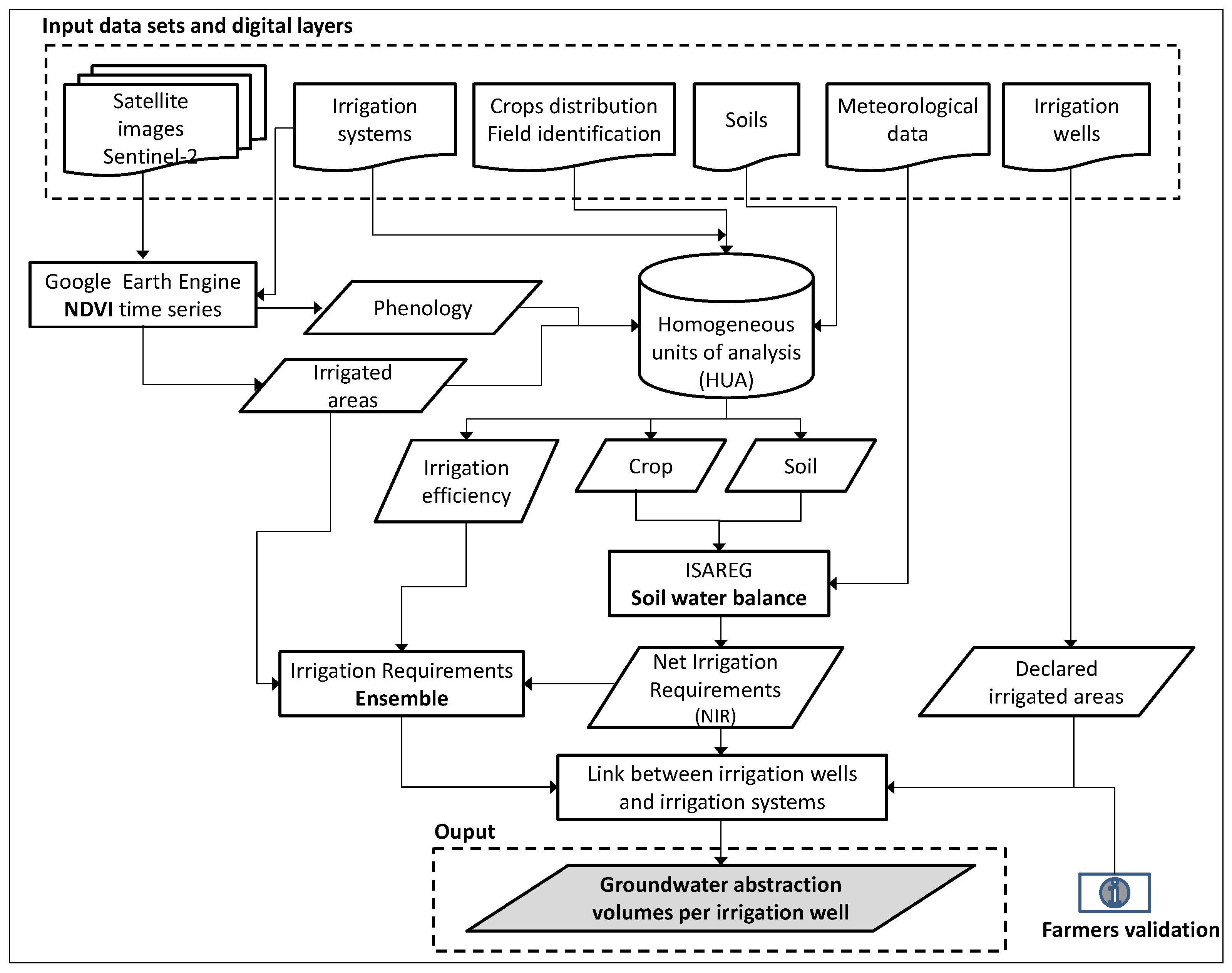
2.2. Methodological Framework for Estimating Groundwater Abstractions per Irrigation Well

The developed methodology is designed to enable the indirect estimation of groundwater abstractions from individual irrigation wells, which may supply one or multiple irrigation systems. It comprises the following core components: (a) estimation of crop water requirements; (b) estimation of irrigation requirements (IR) at the level of each irrigation system; (c) establishment of the spatial correspondence between irrigation systems and their associated wells; and (d) estimation of abstraction volumes per irrigation well. A schematic representation of the methodological workflow is provided in Figure 2.

2.2.1. Applied Datasets and Digital Layers and Their Sources

The datasets and spatial layers necessary for implementing the methodology, along with the corresponding sources of information, are summarized in Table 1.

2.2.2. Crop Data Processing

Crop parameter extraction was performed using time series of the Normalized Difference Vegetation Index (NDVI) [38], derived from Sentinel-2 imagery with a spatial resolution of 10 m and a revisit time of 5 days [39]. These satellite images were integrated with land use maps to confirm the crop types irrigated by each system. The satellite imagery was accessed through the Google Earth Engine (GEE) platform [40], which provides Level-2A Sentinel-2 bottom-of-atmosphere surface reflectance data, including atmospheric corrections. Monthly average NDVI images are used to delineate representative cultivated areas, excluding pixels affected by edge effects. Once these representative crop areas are defined, a time series graph is generated for each, illustrating the evolution of median NDVI values throughout the cropping cycle. This approach enables the estimation of the onset of key crop phenological stages.

Table 1. Datasets and digital layers used in the present work and potential sources.

Category	Datasets and Digital Layers	Source
Meteorology	Air temperature Relative humidity Wind speed Solar radiation Precipitation	National Water Resources Information System (SNIRH)—Portuguese Environment Agency, APA Portuguese Institute for Sea and Atmosphere, IPMA Agrometeorological System for Irrigation Management in Alentejo (SAGRA_COTR)
Crops	Crop identification Phenological stages Crop coefficients Maximum rooting depths Water stress coefficient Readily available water fraction	Field Identification System (iSIP)—Institute for the Financing of Agriculture and Fisheries, IFAP High-resolution satellite imagery—Sentinel-2, Google Earth Engine (GEE) FAO-56 [41] [42,43]
Irrigation	Type of irrigation system Irrigation system efficiency	Google Earth Pro (GEP)—Google [44]
Soils	Soil families Field capacity Wilting point Layer thickness	National Soil Information System (SNIS) –Ag and Rural Development (DGADR) [45] INFOSOLO—National Institute for Agricultural and Veterinary Research (INIAV)
Irrigation wells (validation)	Location Irrigated Area Volumes abstracted	Data provided by farmers

Table 1. Datasets and digital layers used in the present work and potential sources.

Category	Datasets and Digital Layers	Source
Meteorology	Air temperature Relative humidity Wind speed Solar radiation Precipitation	National Water Resources Information System (SNIRH)—Portuguese Environment Agency, APA Portuguese Institute for Sea and Atmosphere, IPMA Agrometeorological System for Irrigation Management in Alentejo (SAGRA_COTR)
Crops	Crop identification Phenological stages Crop coefficients Maximum rooting depths Water stress coefficient Readily available water fraction	Field Identification System (iSIP)—Institute for the Financing of Agriculture and Fisheries, IFAP High-resolution satellite imagery—Sentinel-2, Google Earth Engine (GEE) FAO-56 [41] [42,43]
Irrigation	Type of irrigation system Irrigation system efficiency	Google Earth Pro (GEP)—Google [44]
Soils	Soil families Field capacity Wilting point Layer thickness	National Soil Information System (SNIS) –Ag and Rural Development (DGADR) [45] INFOSOLO—National Institute for Agricultural and Veterinary Research (INIAV)
Irrigation wells (validation)	Location Irrigated Area Volumes abstracted	Data provided by farmers

Based on this information, crop coefficient (Kc) curves were developed for each crop by assigning representative Kc values to the corresponding phenological stages. Earth observation is frequently employed to retrieve crop parameters such as the mean crop coefficient (Kc) or the basal crop coefficient (Kcb), both of which are essential for estimating crop evapotranspiration in accordance with the FAO methodology [41]. These coefficients are often derived empirically from NDVI time series using methods such as those proposed by [46,47]. However, the applicability of such approaches is typically constrained to the specific conditions under which they were developed. In such contexts, NDVI time series prove instrumental in delineating crop development stages, as demonstrated by [48]. Representative Kc values may then be sourced from the literature or adopted from tabulated FAO values [41] and subsequently adjusted to account for local climatic conditions. In the present study, for validation purposes, Kc values of 0.3, 1.1, and 0.2 were used for the initial, mid-season, and late stages of development of maize, respectively, following the methodology of [49].

2.2.3. Irrigation Requirement Estimates Derived from an Ensemble Approach

Homogeneous Units of Analysis (HUA) [50] are defined as spatial areas in which crop type, soil reference group, and irrigation system remain constant. Each HUA represents a spatially coherent area with uniform biophysical and management conditions and is used as the modelling unit in the simulation of the soil water balance to estimate net irrigation requirements (NIR). The spatial distribution of irrigation systems was derived using high-resolution Google satellite imagery and subsequently confirmed through on-site field visits to verify the location and extent of each system. HUA are delineated within a GIS environment by intersecting crop, soil map, and irrigation system layers.

The soil water balance model ISAREG [51] was applied to each HUA to estimate net irrigation requirements (NIR_HUA) according to the following equation:

$${\mathrm{N}\mathrm{I}\mathrm{R}}_{\mathrm{H}\mathrm{U}\mathrm{A}}=∆\mathrm{S}+\mathrm{P}\mathrm{e}+\mathrm{E}\mathrm{T}\mathrm{c}+\mathrm{D}\mathrm{P}+\mathrm{R}\mathrm{O}$$

(1)

where ΔS is the variation in soil water storage, Pe is the effective precipitation, ETc is the crop evapotranspiration, DP is deep percolation, and RO is runoff. All terms are expressed in mm day⁻¹.

ISAREG is based on the FAO-56 methodology [41], in which crop water requirements are calculated using the crop coefficient approach, according to the following equation:

$${ET}_c=ETo Kc$$

(2)

where ET_c is the crop evapotranspiration (mm day⁻¹), ETo is the reference evapotranspiration (mm day⁻¹), and Kc is the crop coefficient.

Our approach incorporates the following simplifications: (i) surface runoff is assumed to be negligible (RO ≈ 0); (ii) each irrigation event is triggered as soon as soil water storage reaches the readily available water threshold. Similar applications of this modelling framework for estimating groundwater abstraction can be found in the studies by [52,53].

Each irrigation system may encompass several HUA. Therefore, the net irrigation requirement for the crop under the irrigation system j (NIR_j, mm) is calculated as follows:

$${\mathrm{N}\mathrm{I}\mathrm{R}}_{\mathrm{j}}={\displaystyle \frac{{{\sum _{\mathrm{i}=1}^{\mathrm{n}}{{(\mathrm{N}\mathrm{I}\mathrm{R}}_{\mathrm{H}\mathrm{U}\mathrm{A}}}_{\mathrm{i}}\times \mathrm{A}\mathrm{r}\mathrm{e}\mathrm{a}}_{\mathrm{H}\mathrm{U}\mathrm{A}}}_{\mathrm{i}})}{{\mathrm{A}\mathrm{r}\mathrm{e}\mathrm{a}}_{\mathrm{j}}}}$$

(3)

where j refers to the irrigation system, n is the number of HUA covered by irrigation system j, i denotes the i-th HUA, NIR_HUA (mm) is the net irrigation requirement for each HUA, Area_HUA (ha) is the area of each HUA, and Area_j (ha) is the area irrigated by the system j.

Irrigation requirements (IR) are then determined by adjusting the previous results according to the irrigation system efficiency, as follows:

$${\mathrm{I}\mathrm{R}}_{\mathrm{j}}={\displaystyle \frac{{\mathrm{N}\mathrm{I}\mathrm{R}}_{\mathrm{j}}}{{\mathrm{E}\mathrm{a}}_{\mathrm{j}}}}$$

(4)

where j refers to the irrigation system, IR is the irrigation requirement (mm), NIR is the net irrigation requirement (mm), and Ea is the application efficiency of the irrigation system (expressed as a fraction) [44].

To account for uncertainties and to generate more robust and reliable estimates of irrigation requirements, an ensemble approach was adopted. The aim of this ensemble is to encompass a plausible range of values for key input parameters that, in the absence of observed data, are associated with greater uncertainty. A sensitivity analysis was performed by applying small percentage variations to these parameters, namely the soil water storage at the time of sowing and the irrigation system efficiency, in order to assess their influence on the output (groundwater abstraction per irrigation well) and to justify their inclusion in the ensemble. The ensemble incorporates the following key parameters:

(i)

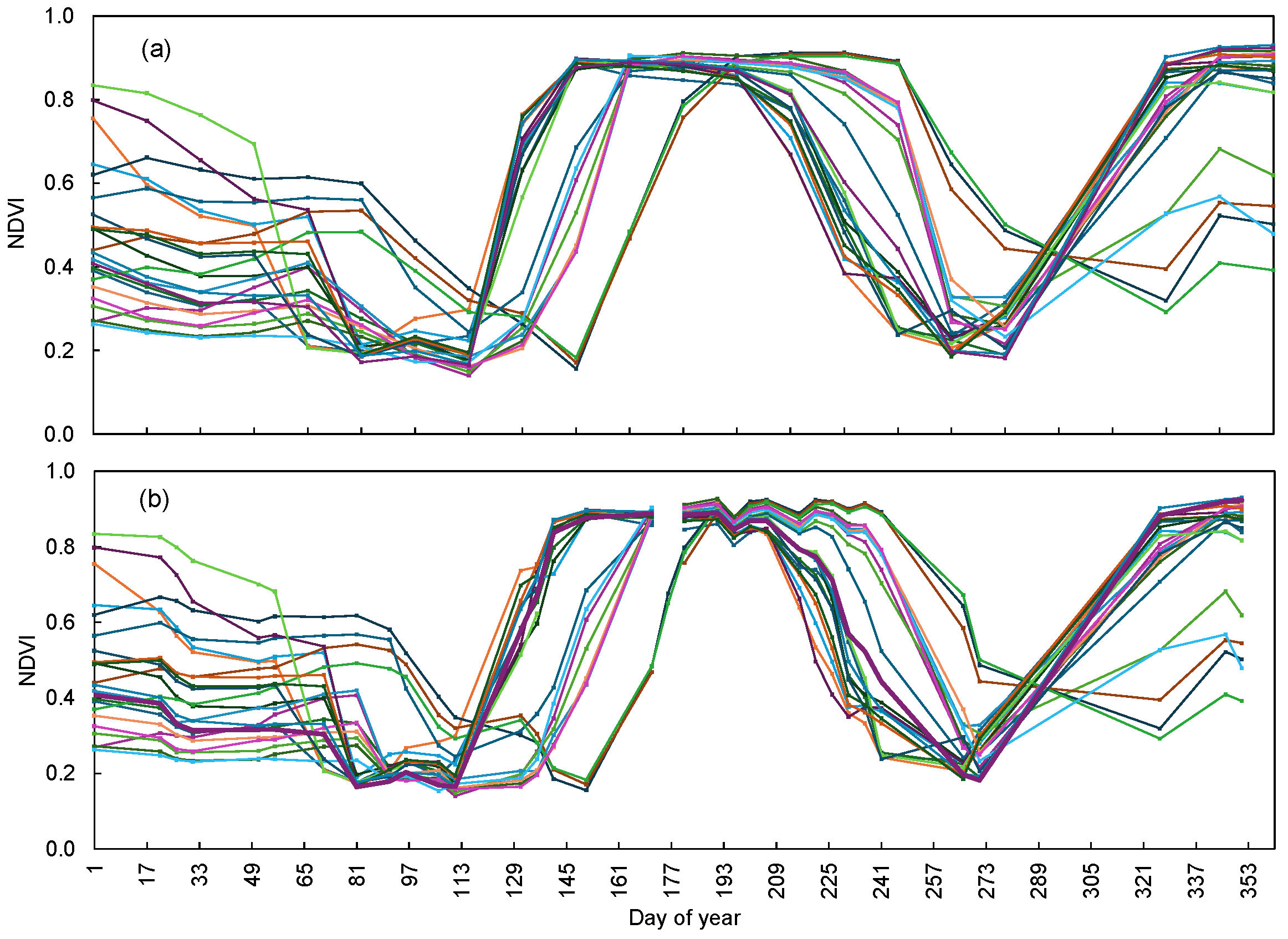
The timeline of crop growth stages is one of the primary sources of uncertainty when estimating crop evapotranspiration, and thus, when calculating irrigation requirements, as noted by [41]. To address this, satellite imagery with average revisit intervals of 5 days (TS5) and 16 days (TS16) was used to estimate crop cycles based on RS data acquired over different temporal resolutions. NDVI time series were generated in Google Earth Engine (GEE) for both aggregation intervals, enabling a complementary analysis of crop phenology. Minor discrepancies, typically a few days, between the two series may occur, leading to corresponding differences in the crop coefficient curves derived for each case.

(ii)

Soil water storage at the onset of the irrigation season is a key variable influencing the soil water balance and, consequently, irrigation scheduling. The extent of soil moisture depletion prior to sowing depends on the timing of the sowing period relative to the end of the antecedent rainy season. In this study, spring crops are typically sown during a period characterized by high rainfall variability and substantial water demand, making it challenging to assign a definitive value for soil water storage at sowing. To account for this uncertainty, two scenarios were considered in the ensemble: a conservative scenario assuming 30% of the available soil water (ASW) at sowing, reflecting drier initial conditions; and a scenario assuming 80% of ASW at sowing, representing more favorable initial conditions. For the deeper soil layers (>0.4 m deep), 70% of ASW was assumed in both scenarios.

(iii)

Irrigation system application efficiency is another parameter subject to considerable uncertainty, particularly in the absence of field-based performance assessments. This uncertainty arises from factors such as ageing infrastructure, suboptimal system design, and inadequate maintenance. Accordingly, two contrasting efficiency values were considered for each irrigation system, based on ranges reported in the literature: one representing poorly maintained or degraded systems with low efficiency, and the other representing well-maintained and properly designed systems operating close to their theoretical potential.

2.2.4. Estimation of Groundwater Abstraction per Irrigation Well

The inherent complexities of irrigation water management make it unfeasible to quantify water use from an individual irrigation based solely on satellite data. For example, a single well may supply water to several irrigation systems, while a single irrigation system may be fed by multiple wells. Consequently, establishing a reliable correspondence between the points of water abstraction and the sites of water application was essential, a task that has previously been recognized as particularly challenging [54]. To address this challenge, a multi-stage approach was implemented. Firstly, spatial data on irrigation infrastructure, obtained from high-resolution satellite imagery and corroborated through field surveys, were employed to delineate the physical extent of each irrigation system. Second, irrigation wells were geo-referenced using official registries, which were subsequently complemented and corrected using ground-truthing. Finally, the correspondence between wells and irrigation systems was established through a combination of spatial proximity analysis within a GIS environment and field-level validation involving farmers, who provided information on actual water distribution practices. This approach, illustrated in Figure 3, enabled the assignment of each irrigation system to its most probable set of contributing wells, thereby facilitating a more accurate estimation of groundwater abstractions at the system level.

Figure 4 presents a schematic diagram illustrating possible associations between irrigation wells and irrigation systems. Assuming that in cases involving multiple abstraction points, each well contributes equally to satisfying the irrigation requirements of a given system, the estimated groundwater abstraction volume (GA_Ek, m³) attributable to irrigation well k is calculated as follows:

$${\mathrm{G}\mathrm{A}}_{\mathrm{E}\mathrm{k}}=\sum _{\mathrm{j}=1}^{\mathrm{n}}{\displaystyle \frac{{{\mathrm{I}\mathrm{R}}_{\mathrm{j}}\times \mathrm{A}}_{\mathrm{j}}}{{\mathrm{C}}_{\mathrm{j}}}}$$

(5)

where GA_Ek is the estimated groundwater abstraction volume at irrigation well k (m³); n is the number of irrigation systems supplied by well k; IR_j is the requirement of the irrigation system j (mm) (Equation (4)); A_j is the area irrigated by system j (ha); C is the number of wells supplying irrigation system j.

2.2.5. Assessment of Methodological Accuracy in a Real Irrigation Context

Despite the constraints associated with limited data availability, we were able to collaborate with a small number of large-scale farmers operating three distinct irrigation system types, solid-set sprinkler, center-pivot, and drip irrigation, operating on different soil types (Regosols, Fluvisols, and Luvisols). This combination enabled the methodology to be tested under varied agronomic and pedological conditions, representing a valuable opportunity for validation within the context of data scarcity.

The methodology was validated using observed groundwater abstraction volumes (GA_O, m³), obtained from flowmeters installed at selected abstraction points, specifically, those where farmers consent to share both water use data and information on the areas irrigated by each well. To safeguard the privacy of participating farmers, field locations are presented solely at the spatial resolution of the Tagus Vulnerable Zone.

The accuracy of the estimates was assessed through both visual and statistical comparisons, employing the following performance indicators:

(a)

Coefficient of Determination (R²): This coefficient quantifies the proportion of variability in the dependent variable that is explained by the regression model. Its values range from 0 to 1, with R² = 1 indicating that the model accounts for 100% of the variance in the observed data, and R² = 0 indicating that it explains none. It is computed as follows [55]:

$${\mathrm{R}}^2={\displaystyle \frac{\sum _{z=1}^n{({GA}_{Rz}-\overline{{GA}_E})}^2}{\sum _{z=1}^n{({GA}_{Ez}-\overline{{GA}_E})}^2}}$$

(6)

where GA_Rz is the groundwater abstraction volume predicted by the regression model for sample z; GA_Ez is the groundwater abstraction volume estimated by the methodology for sample z; $\overline{GA}$_R is the mean of the regression-based abstraction values; $\overline{GA}$_E is the mean of the estimated abstraction volumes; n is the number of observations.

(b)

Root Mean Square Error (RMSE): This metric represents the average magnitude of the differences between estimated and observed values. A lower RMSE indicates better model performance, as it reflects smaller average prediction errors. It is calculated as follows [55]:

$$\mathrm{R}\mathrm{M}\mathrm{S}\mathrm{E}=\sqrt{{\displaystyle \frac{\sum _{\mathrm{z}=1}^{\mathrm{n}}{({\mathrm{G}\mathrm{A}}_{\mathrm{E}\mathrm{k}}-{\mathrm{G}\mathrm{A}}_{\mathrm{O}\mathrm{k}})}^2}{\mathrm{n}}}}$$

(7)

where GA_Ok is the observed abstraction volume for the irrigation well k; n is the number of observations.

3. Results and Discussion

3.1. Spatial Distribution of Soils and Irrigation Systems

Figure 5a presents the spatial distribution of irrigation systems across the study area. The predominant system is center-pivot irrigation (9 systems), which accounts for approximately 64% of the total irrigated area under consideration. This is followed by solid set sprinkler systems (13 systems), covering around 35% of the area. Drip irrigation systems (2 systems) represent the smallest share, occupying only 1% of the total area.

Figure 5b shows the spatial distribution of soil reference groups (WRB) within the study area. Among the identified groups, Fluvisols (medium-textured, non-calcareous) are predominant, covering approximately 60% of the area analyzed. In this figure, soil information is aggregated at the WRB group level to improve readability. However, a higher level of detail, corresponding to the soil family level in the Portuguese soil classification, was employed in the definition of the HUA.

3.2. Crop Biophysical Parameters

3.2.1. NDVI

Figure 6 presents the Normalized Difference Vegetation Index (NDVI) time series derived from Sentinel-2 imagery, using 16-day median composites (Figure 6a) and 5-day composites (Figure 6b). The 16-day NDVI time series (TS16) exhibits a lower incidence of missing observations compared to the 5-day series (TS5), a pattern consistent with the compositing strategies employed. While TS5 composites typically rely on individual Sentinel-2 acquisitions, making them highly susceptible to cloud cover, the TS16 series benefits from temporal aggregation, which enhances robustness by incorporating multiple observations within each compositing interval.

Preliminary analysis of NDVI temporal trajectories, assessing amplitude, seasonal dynamics, and phenological landmarks such as greening onset and peak biomass, enabled the identification of maize as the cultivated crop. The use of vegetation index time series, particularly NDVI, derived from satellite data, is a widely validated approach for crop classification. For example, Ref. [56] employed Landsat-derived NDVI and land surface temperature metrics to classify crops in the Tagus basin using machine learning algorithms, while [52] differentiated seasonal classes of irrigated crops in La Mancha, Spain, and linked these classifications to estimates of groundwater abstraction.

From a phenological perspective, early growth stages were more clearly discernible in the TS5 series, particularly under late sowing conditions, where thermal accumulation accelerates development and shortens the low-NDVI phase typically associated with soil disturbance and sowing. This phase is often masked in the TS16 series due to the temporal smoothing effect of the composition process.

As illustrated in Figure 7, for the case of the irrigation system Pivot 7, the initial vegetative stage is clearly identifiable in the TS5 series (Figure 7a) but not in TS16 (Figure 7b), likely due to a data gap between day of year (DOY) 151 and 171. Such differences are attributable to the compositing methodology: the median filter applied in the 16-day aggregation suppresses short-term NDVI fluctuations, reducing noise and enhancing interpretability during stable phases of crop development. However, this smoothing effect can obscure subtle transitions, such as sowing, which are critical for accurate phenological characterization. Conversely, for later growth stages, the smoothing introduced by the TS16 series can be advantageous. In the case of the Solid Set Irrigation System 12, the end of the intermediate growth phase is poorly resolved in TS5 (Figure 7c), whereas the TS16 series (Figure 7d) enables a clearer identification, with DOY 209 emerging as the likely transition point.

The analysis of NDVI time series extracted for each HUA revealed both similarities and contrasts in phenological trajectories. Based on the 5-day composite series (TS5), nine distinct phenological development cycles were identified, primarily distinguished by differences in sowing dates and the timing of key growth stages. To account for this variability, a phenology-based segmentation approach was employed, treating each temporal pattern as a distinct crop instance. This approach is consistent with established time-series clustering methods commonly used to differentiate cropping practices based on intra-seasonal spectral dynamics. As a result, nine individual grain maize crop cycles were identified and characterized and are hereafter referred to as Maize 1 through 9.

In contrast, the 16-day composite series (TS16) enabled the identification of only seven distinct crop cycles. These cycles appeared shorter in duration than those detected using the TS5 series, a difference mainly attributed to the lower temporal resolution and the smoothing effect inherent in the 16-day median compositing process. Such aggregation tends to mask short phenological phases, such as sowing, emergence, and flowering, particularly when these occur between satellite acquisition dates, potentially leading to an underestimation of the actual crop cycle duration. Furthermore, the lower frequency of cloud-free observations in TS16 reduced the capacity to capture subtle inter-field variations, thereby limiting the ability to discriminate between individual cropping patterns. Seven grain maize crop cycles were identified and characterized, hereafter designated as Maize 1 through 7.

Previous work by [56] demonstrated that Landsat imagery, despite its coarser temporal (16-day) and spatial (30-m) resolution, provides a suitable foundation for monitoring crop phenology. However, it was also noted that sensors with finer revisit intervals and higher spatial resolution can significantly enhance the detection of short-duration phenological phases and intra-field variability. This perspective is further supported by [57,58,59], who likewise emphasized the value of high-frequency NDVI data for capturing phenological events with greater precision. The findings of the present study corroborate these observations, demonstrating that Sentinel-2 imagery improves both temporal continuity and spatial detail, particularly during critical transitions such as sowing and early vegetative development. The results confirm the utility of Sentinel-2 NDVI time series for monitoring grain maize, enabling reliable crop identification and precise detection of key phenological stages, while also highlighting the inherent trade-off between temporal resolution and noise reduction in remote sensing-based crop monitoring. Nonetheless, some limitations should be acknowledged. NDVI tends to saturate at peak biomass, diminishing its sensitivity to physiological changes during later growth stages. Additionally, phenological detection remains dependent on the availability of cloud-free imagery, and even with a 5-day revisit frequency, persistent cloud cover, particularly in spring, can obscure short-duration phenological events.

Despite these challenges, characterizing crop cycles, especially sowing and harvesting dates, using remote sensing time series has proven to be more accurate than relying on standard tabulated values (e.g., [41]). This has been demonstrated by [46,60], who showed that satellite-derived phenological metrics provide a more site-specific and temporally accurate depiction of crop development, capturing interannual variability and the influence of local management practices.

3.2.2. Crop Coefficient Curves

Figure 8 presents the crop coefficient (Kc) curves derived from the nine and seven crop cycles identified using the TS5 and TS16 mean composite time series, respectively. The TS5 series revealed four distinct sowing dates, while three were identified in the TS16 series. In both cases, a progressive shortening of the initial crop development phase was observed with later sowing dates, as expected due to rising temperatures during that period. Analysis of the Kc curves derived from the TS5 indicates that aside from variation in the early development stage, the overall duration of the crop cycles remained relatively constant across the different maize instances. In contrast, the Kc curves generated from the TS16 series exhibited greater variability, particularly during the intermediate and late growth phases, reflecting a more pronounced delineation of these stages, as previously discussed.

3.3. Homogeneous Units of Analysis

The criteria for delineating the Homogeneous Units of Analysis (HUA), particularly in relation to thresholds for uniformity in crop types, soil reference groups, and irrigation systems were as follows: crop types were differentiated based on discernable variations in the NDVI values derived from satellite imagery for both the 5-day and 16-day median composite series, as previously described. With respect to soils, classification was not based on specific soil parameters but rather on the soil map employed, which identifies three soil reference groups (Regosols, Fluvisols, and Luvisols). This soil map was incorporated into the analysis as a GIS layer, allowing for spatial overlay with other datasets. In the case of irrigation systems, the thresholds were explicitly defined according to the system type, namely center-pivot, solid-set sprinkler, and drip irrigation, as detailed in

Table 2. Net irrigation requirements for each Homogeneous Unit of Analysis, derived from 5-day NDVI mean composite time series, considering initial root zone soil water storage of 30% and 80% of available water at sowing (2023).

HUA	Crop	Soil *	IS	NIR		HUA	Crop	Soil *	IS	NIR
				30%	80%					30%	80%
1	M3	RG	SS8	435	429	21	M3	FL	P1	433	428
2	M3	RG	SS8	432	425	22	M9	FL	SS 4	390	381
3	M3	RG	SS6	435	429	23	M9	FL	SS4	397	391
4	M8	FL	SS3	481	476	24	M8	FL	P3	481	476
5	M2	FL	SS12	452	445	25	M8	LV	P3	480	472
6	M6	FL	P8	455	445	26	M4	FL	P2	440	434
7	M6	FL	P8	461	455	27	M4	FL	SS1	440	434
8	M9	FL	P9	390	381	28	M4	LV	P2	438	431
9	M9	FL	P9	390	382	29	M4	FL	DI2	440	434
10	M9	FL	P9	397	391	30	M4	LV	DI2	438	431
11	M1	FL	SS10	446	438	31	M7	FL	P6	484	479
12	M2	FL	SS11	452	445	32	M7	FL	P5	484	479
13	M1	FL	SS9	446	438	33	M8	FL	SS13	481	476
14	M1	RG	SS9	454	448	34	M8	LV	SS13	480	472
15	M4	FL	SS5	433	425	35	M8	FL	SS2	481	476
16	M4	RG	SS5	441	435	36	M8	FL	P4	481	476
17	M9	FL	P7	390	381	37	M8	LV	SS2	480	472
18	M9	FL	P7	397	391	38	M8	FL	DI1	475	465
19	M5	FL	SS7	424	417	39	M8	FL	DI1	481	476
20	M5	RG	SS7	430	422	40	M8	LV	P 4	480	472

HUA = Homogeneous Unit of Analysis; IS = irrigation system; NIR = net irrigation requirements; M = maize; P = pivot; SS = solid set; DI = drip irrigation systems; * WRB Reference Soil Groups: FL = Fluvisols; RG = Regosols; LV = Luvisols.

and

Table 3. Net irrigation requirements for each Homogeneous Unit of Analysis, derived from 16-day NDVI mean composite time series, considering initial root zone soil water storage of 30% and 80% of available water at sowing (2023).

HUA	Crop	Soil *	IS	NIR		HUA	Crop	Soil *	IS	NIR
				30%	80%					30%	80%
1	M1	RG	SS8	423	417	21	M1	FL	P1	422	416
2	M1	RG	SS8	419	413	22	M7	FL	SS4	401	392
3	M1	RG	SS6	423	417	23	M7	FL	SS4	407	402
4	M5	FL	SS3	463	457	24	M5	FL	P3	463	457
5	M2	FL	SS12	437	429	25	M5	LV	P3	461	454
6	M4	FL	P8	432	423	26	M2	FL	P2	444	439
7	M4	FL	P8	438	433	27	M2	LV	P2	442	435
8	M7	FL	P9	401	392	28	M2	FL	DI2	444	439
9	M7	FL	P9	400	393	29	M2	LV	DI2	442	435
10	M7	FL	P9	407	402	30	M 2	FL	SS1	444	439
11	M1	FL	SS10	415	407	31	M5	FL	P6	463	457
12	M2	FL	SS11	437	429	32	M5	FL	P5	463	457
13	M1	FL	SS9	415	407	33	M5	FL	SS13	463	457
14	M1	RG	SS9	423	417	34	M5	LV	SS13	461	454
15	M2	FL	SS5	437	429	35	M6	FL	SS2	537	457
16	M2	RG	SS5	445	439	36	M6	LV	SS2	535	454
17	M7	FL	P7	401	392	37	M5	FL	DI1	456	447
18	M7	FL	P7	407	402	38	M5	FL	DI1	463	457
19	M3	FL	SS7	428	421	39	M5	FL	P4	463	457
20	M3	RG	SS7	434	427	40	M5	LV	P4	461	454

HUA = Homogeneous Unit of Analysis; IS = irrigation system; NIR = net irrigation requirements; M = maize; P = pivot; SS = solid set; DI = drip irrigation systems; * WRB Reference Soil Groups: FL = Fluvisols; RG = Regosols; LV = Luvisols.

. The intersection of this spatial information resulted in the delineation of 40 HUA. The units identified from the TS5 series are presented in Table 2. The two largest units in terms of spatial extent are HUA 21 (Pivot 1 × Maize 3 × fluvisols), covering 11.3% of the study area, and HUA 24 (Pivot 3 × Maize 8 × fluvisols), which occupies 11.0%. A comparison of the HUA derived from TS5 and TS16 (Table 3) reveals a high degree of agreement in identifying the most spatially dominant units, thereby supporting the robustness of the spatial framework used for HUA delineation, irrespective of the temporal resolution. Nonetheless, minor discrepancies in crop assignment (e.g., Maize 3 vs. Maize 1; Maize 8 vs. Maize 5) underscore the sensitivity of phenological classification to temporal resolution, with the 5-day series offering finer intra-seasonal detail.

3.4. Irrigation Requirements

Figure 9 presents the results, obtained for three wells of the sensitivity analysis conducted for two key factors influencing the estimation of irrigation requirements and consequently, groundwater abstraction: soil water storage at sowing as a percentage of the available soil water (%ASW) (top graphs) and the irrigation system application efficiency (Ea) (bottom graphs). As expected, the estimated abstraction volumes decreased progressively with increasing %ASW at sowing. On average, a 10% increase in soil water storage at sowing resulted in a reduction in groundwater extraction of 1.55%, 1.47%, and 1.98% for wells C5, C15, and C18, respectively, corresponding to absolute decreases of 954.5 m³, 1479.4 m^3, and 904.2 m³. With respect to application efficiency (Ea), the percentage variation in estimated abstraction volumes was consistent across the three wells, with an overall average reduction of 6.48% per 10% of efficiency increase. The corresponding absolute decreases in abstraction volumes were 4448.2 m³, 7462.9 m^3, and 3193.1 m³ for wells C5, C15, and C18, respectively. At this level of analysis, focused on estimating groundwater abstraction per well, these variations are considered meaningful and support the inclusion of both parameters within the ensemble framework.

Building on the findings of the sensitivity analysis, the ensemble was developed by conducting simulations under two contrasting assumptions for soil water storage at sowing: 30% and 80% of the soil’s available water capacity. With respect to irrigation system application efficiency, calculations were performed for two values for each irrigation system type: 65% and 75% for solid-set systems, 70% and 85% for center-pivot systems, and 75% and 95% for drip irrigation.

Irrigation requirements were computed using the ISAREG soil water balance model, incorporating crop parameters derived from remote sensing, soil data (Tables S1 and S2), and local meteorological observations.

Net irrigation requirements (NIR) for each HUA are presented in Table 2 and Table 3 for the 5-day (TS5) and 16-day (TS16) NDVI composite series, respectively. In general, higher NIR values are associated with crops sown later in the season, where the intermediate growth stage coincides with the high atmospheric evaporative demand of July and August. Exceptions include Maize 9 (Table 2) and Maize 7 (Table 3), which, due to their shorter development cycles, exhibited lower-than-expected irrigation requirements. A comparison of the results obtained from the 5-day and 16-day NDVI median composite time series (Table 2 and Table 3) shows that in most HUA, net irrigation requirements (NIR) are lower when derived from the 16-day series. This is mainly due to the shorter crop development cycles identified in the 16-day dataset, which result in reduced seasonal water demand.

The apparent shortening of the crop cycle is attributable to the temporal smoothing effect of compositing, which can obscure short-duration phenological stages and compress or shift the detection of key growth transitions. Consequently, NIR estimates based on the 16-day series may underestimate actual water demand, particularly when early or intermediate phases are not fully represented.

This approach produced an ensemble of eight irrigation requirement (IR) estimates for each of the 24 irrigation systems. The resulting IR ensembles are presented in Figure 10, disaggregated by irrigation system. The overall mean IR was 576 mm with a standard deviation of ±56 mm. When disaggregated, the mean values were 561 ± 57 mm for center-pivot systems, 593 ± 52 mm for solid-set sprinklers, and 535 ± 42 mm for drip irrigation systems.

The spatial distribution of seasonal irrigation requirements (IR) across the study area reveals variability, largely driven by differences in crop phenology and irrigation system characteristics. As illustrated in Figure 10, lower IR values were recorded for Pivot 7 (P7), Pivot 9 (P9), and Solid Set Sprinkler 4 (SS4). These systems irrigated Maize Crop 9, which is characterized by a shorter development cycle, thereby reducing seasonal water demand. In contrast, Solid Set Sprinkler 2 (SS2) exhibited the highest IR value among all system–crop combinations. This can be attributed to its association with Maize Crop 6, whose extended intermediate phase resulted in a higher cumulative evapotranspiration and thus greater irrigation requirements.

These findings highlight the influence of intra-seasonal phenological variability on irrigation demand, even within relatively homogeneous agro-climatic conditions. The integration of remote sensing-derived crop information into irrigation requirement assessments provided a valuable means to capture such heterogeneity, enabling more precise water resource planning and management [60,61].

3.5. Groundwater Abstraction Volumes

Table 4. Association between irrigation wells (IW) and supplied irrigation systems.

IW	IS		Ae (ha)	IW	IS		Ae (ha)
IW1	P3	DI1	12.4	IW11	P9	SS4	13.6
IW2	P3	DI1	12.4	IW12	SS7		9.4
IW3	P4 SS3	SS13	11.8	IW13	SS7		9.4
IW4	SS2		10.0	IW14	SS8		9.8
IW5	P2 SS1	DI2	11.3	IW15	P6		17.9
IW6	P1		7.9	IW16	SS9 SS10 SS11	SS12 SS6	6.3
IW7	P1		7.9	IW17	P8		9.7
IW8	P1		7.9	IW18	SS5		8.1
IW9	P7		18.8	IW19	SS9 SS10 SS11	SS12 SS6	6.3
IW10	P5		11.4	IW20	SS9 SS10 SS11	SS12 SS6	6.3

IW = irrigation well, IS = irrigation system, Ae = estimated area.

provides the linkage between groundwater abstraction points, the irrigation systems they supply, and the corresponding irrigated areas according to the workflow provided in Figure 3. It is evident that certain irrigation wells (IW) serve multiple irrigation systems. For example, IW1 supplies both a center-pivot and a drip irrigation system, while IW16 supplies five solid-set sprinkler systems, among others. Conversely, there are also irrigation system × crop combinations that are supplied by more than one abstraction point. This is the case for P1, which is supplied by IW6, 7, and 8, and for solid-set sprinkler SS9, which receives water from IW16, 19, and 20. This configuration reveals a complex groundwater use network, where both multi-source and multi-demand relationships coexist. This challenges the accurate monitoring of abstractions and the attribution of water use to specific practices or crop types. Moreover, it complicates the implementation of water accounting frameworks and the design of effective management strategies, particularly in contexts where regulatory oversight is limited or where metering is absent.

The presence of shared abstraction points underscores the need for integrated water management approaches that consider the cumulative impacts of multiple users and systems drawing from the same resource. In this context, spatially explicit tools that couple crop-level irrigation requirements with well-level abstraction data are essential to improve resource-use efficiency and ensure long-term aquifer sustainability.

Groundwater abstraction for irrigation (GA_Ek) for the 2023 season was estimated using Equation (4), yielding an ensemble of eight values per irrigation well (Figure 11). The box plots represent the distribution of simulated abstraction volumes for each well based on the ensemble approach. This visualization enables comparison between modelled estimates and observed values, while capturing the uncertainty associated with key input parameters.

Abstracted volumes ranged from approximately 33,000 m³ for irrigation wells 16, 19, and 20, to 115,000 m³ for irrigation well 15. The latter supplies Pivot 6, which irrigates 17.0 ha of maize grown on a Fluvisol [35]. In contrast, wells 16, 19, and 20 collectively supply a total of 6.3 ha via solid-set systems. In addition, the variation in crop development cycles identified across the study area also influenced the estimated abstraction volumes. For example, IW4 and 14 both supply solid-set sprinkler systems irrigating similar areas (Table 4). However, IW4 supplies a crop sown later in the season compared to the crop associated with IW14, resulting in higher irrigation water requirements. This is because the crop irrigated by IW4 has its intermediate phase, when water demand is highest, coinciding with the peak summer months (July and August), whereas the crop irrigated by IW14 undergoes its intermediate phase during late May to early July, when climatic demand is comparatively lower.

Results reveal substantial variation in the volumes extracted among irrigation wells, reflecting the heterogeneous nature of water use intensity across the study area, shaped by differences in irrigation system types, crop water demands, and land use patterns.

By linking remotely sensed crop irrigation requirements to the spatial configuration of the abstraction network, the method enables robust, distributed estimates of groundwater use. These outputs are particularly valuable in regions where direct metering data are lacking or incomplete, offering a science-based alternative for supporting aquifer-scale water balance assessments. The method enhances the capacity to identify potential overexploitation risks and provides a decision-support tool for water allocation planning, licensing regulation, and the spatial prioritization of monitoring efforts in high-demand areas.

3.6. Validation of the Methodology for the Case Study

Figure 11 also compares the estimated groundwater abstractions (GA_Ek) with the observed abstractions (GW_O) derived from flowmeter readings installed at the irrigation wells. The results show that for all IW, the range of estimated abstractions encompassed the corresponding observed value. IW9 and 11 supplied Maize Crop M9 (Table 2 and Table 3), which had a shorter growing cycle. As a result, the estimated abstractions for these wells were lower than what would be expected. In contrast, for IW 3, 4, and 10, the estimated average exceeded the observed consumption. This overestimation may be attributed to a mismatch between the soil types assumed in the modelling and the actual field conditions. The soils in these areas were identified as a Fluvisol and a Luvisol, both characterized by low available water (SAW) and typically associated with higher net irrigation requirements. As SAW is a key determinant of irrigation demand, any misclassification can result in considerable deviations in the estimated water use.

The relationship between the areas estimated via remote sensing (A_e) and the officially licensed areas (A_d) is shown in Figure 12a. A strong agreement is observed between the licensed values and those derived from Sentinel-2 NDVI imagery, with a coefficient of determination (R²) of 0.9977 and a regression line slope of 0.985. The results indicate a good fit and no evidence of systematic bias. On average, the remote sensing-based estimates were 0.8% lower than the declared areas. However, in one of the 20 irrigation wells used for methodological validation, a discrepancy greater than 10% was identified. Similar work by Zipper et al. [27] reported satellite-derived irrigation areas that were 6.9% higher than reported values. Given that inaccuracies in estimating irrigated areas can result in under- or overestimation of groundwater abstraction, the strong correlation observed in this study supports the accuracy and reliability of the proposed methodology for the case study.

To assess the accuracy of the estimated abstractions, a linear regression analysis was conducted between the modelled values (GW_E) and the corresponding observations (GW_O) at the irrigation wells. As shown in Figure 12b, the estimated abstraction volumes exhibit a strong linear relationship with the measured values. The regression model explains 91.8% of the variance of the observed data, indicating a high degree of agreement between estimated and measured values. The regression slope is close to one, suggesting that the methodology, overall, does not underestimate or overestimate abstractions, although local deviations were observed at specific wells. The validation further confirms the model’s performance, with an overall RMSE value of 5.45 × 1000 m³, corresponding to 9.3% of the mean observed value for the estimated ensemble. Ott et al. [54] reported RMSE values for the basin-scale pumping volume estimates ranging between 7 and 17% of the reported ones.

Some variability was observed at the level of individual abstraction points, primarily due to differences in crop cycle detection and assumptions regarding soil properties. While the irrigated areas are generally more straightforward to determine than the irrigation depths, the estimates showed strong agreement between estimated and reported values. However, when irrigation volumes were normalized by this area to derive application depth, additional variability was introduced. Nevertheless, the overall performance metrics indicate that the methodology is robust and well-suited for estimating groundwater abstraction for irrigation.

3.7. Sources of Uncertainty in the Proposed Methodology

The methodology relies on several assumptions and simplifications, which introduce uncertainty into the estimation of groundwater abstraction volumes. This is partially addressed through the adoption of an ensemble approach. Nonetheless, the following limitations should be acknowledged.

Crop identification and delimitation: uncertainties arise from inaccuracies in field delineation and crop identification, which affect irrigation requirement (IR) estimates. NDVI tends to saturate at peak biomass, reducing its sensitivity to physiological changes during later stages of crop development. Furthermore, the detection of phenological events remains dependent on the availability of cloud-free imagery. Even with a 5-day revisit interval, persistent cloud cover can obscure short-duration phenological events with a particular impact in autumn-winter crops [50]. Future studies could benefit from integrating complementary indices (e.g., EVI, red-edge bands) or SAR data to improve performance under cloudy conditions and enhance sensitivity across all phenological stages.

Soil Characterization: The generalized soil information derived from the national 1:25,000 soil map introduces uncertainty due to the high spatial variability of soil properties, which directly affects IR estimations. Enhancing the spatial resolution and field validation of soil maps is therefore essential to improve the reliability of remote sensing-based estimates of groundwater abstraction.

Irrigation systems and management: uncertainty also arises from the assumed values of irrigation system efficiency and scheduling, as well as actual field performance. Local practices, such as deficit irrigation or early termination of irrigation before harvest, can substantially influence water use. To account for this variability, a range of system efficiency values was incorporated into the analysis.

Water balance components: The exclusion of runoff and potential misestimation of effective rainfall can affect soil water balance calculations, particularly during the crop establishment phase. To partially address this, a range of soil water storage values at sowing was considered within the ensemble approach.

Linking abstraction points to irrigated areas: establishing spatial associations between wells and irrigated plots presents a significant challenge, as abstraction points may serve multiple irrigation systems and may be located outside the boundaries of the irrigated area. This spatial linkage was identified as one of the primary methodological difficulties in the present study. Similar challenges have been noted in previous research as a major source of uncertainty (e.g., [27,54]). Addressing this issue requires detailed geospatial analysis and participatory validation to improve the reliability of the spatial assignment of abstraction sources to application areas [54].

Other water uses and sources: The methodology assumes that groundwater abstraction is exclusively for irrigation and that groundwater is the sole source of water. In practice, this may not be true. Non-irrigation uses (e.g., livestock, equipment washing) and the presence of alternative sources, including on-farm reservoirs or surface water, may lead to overestimations. To enhance accuracy, complementary data collection through farm surveys and participatory mapping is recommended.

3.8. Applications and Transferability of the Methodology

This approach has multiple potential applications. At the farm level, it enables farmers and irrigation managers to assess whether actual water use aligns with estimated irrigation requirements, thereby identifying potential inefficiencies or excessive losses. In addition, by quantifying the volume of irrigation water applied, it becomes possible to estimate the amount of nitrates introduced through irrigation [62]. This information can inform fertilization planning, potentially reducing overall fertilizer application with clear economic and environmental benefits [63,64]. This supports the adoption of more efficient irrigation and fertilization strategies, ultimately contributing to improving on-farm water management.

The methodology is also applicable to perennial crops, such as olive groves and vineyards, as satellite imagery can effectively detect the transition from dormancy, marking the onset of the irrigation season.

By extrapolating from well-characterized reference sites, the methodology may also be adapted for broader applications in data-scarce contexts, where the detailed spatial linkage between wells and irrigated areas is not required. At the regional scale, the methodology offers a valuable tool for estimating spatially distributed groundwater use in agricultural areas lacking flowmeter data, which is still a common scenario in many regions. This facilitates a better understanding of the broader implications of groundwater abstraction on the agro-hydrological system.

From a water governance perspective, the methodology contributes to aquifer-level assessments by enabling the identification of overexploitation risks, supporting licensing procedures, and informing the prioritization of monitoring and enforcement efforts. In regions where declining groundwater levels have raised sustainability concerns, this approach offers a practical and scalable tool to promote the responsible and equitable use of shared groundwater resources.

4. Conclusions

This study proposes a methodology for the indirect estimation of groundwater abstraction for irrigation at the scale of individual wells, addressing a key gap in current water monitoring practices. By integrating Sentinel-2 NDVI-derived crop phenology, spatially explicit irrigation system characterization, soil information, and soil water balance modelling, the approach enables the estimation of irrigation requirements and corresponding abstraction volumes with high spatial resolution.

A central innovation of this work is the construction of an ensemble of eight abstraction estimates per well. This ensemble captures key sources of uncertainty, namely phenological variability, initial soil water storage, and irrigation system efficiency, thereby improving the robustness and reliability of the estimates.

Groundwater abstraction volumes estimated per well ranged from approximately 33,000 m³ to 115,000 m³ during the 2023 irrigation season, reflecting the combined influence of irrigated area, irrigation system, soil water retention characteristics, and crop development cycle. These results highlight the heterogeneous nature of groundwater use at the local scale and the need for spatially resolved monitoring tools.

Validation against flowmeter data demonstrated strong agreement, with all the values falling within the estimated ensemble range. The method achieved an RMSE of 5.45 × 10³ m³, corresponding to 9.3% of the observed mean volume, underscoring its accuracy even under conditions of limited observed data.

The ability to estimate groundwater abstraction volumes at the level of individual wells represents a substantial advance for irrigation monitoring and groundwater governance. It supports multiple end-users: farmers, who can align water use with crop requirements and optimize fertilizer application; water managers, who can detect inefficiencies and identify zones of overexploitation; regulators, who require reliable estimates for licensing and enforcement in the absence of direct measurements.

Given its reliance on publicly available data and open-source tools, the methodology is transferable and cost-effective. It is particularly relevant in Mediterranean agro-hydrological contexts, where summer crops are heavily reliant on groundwater due to prolonged dry periods.

Future improvements should focus on enhancing the detection of phenological transitions under cloudy conditions, refining soil spatial datasets, and automating the spatial linkage between abstraction points and irrigated plots to facilitate broader implementation. The incorporation of gridded meteorological data (e.g., E-OBS, ERA5) is also planned to address limitations in conventional weather station coverage.

Overall, this methodology provides a scalable solution for groundwater accounting in regions characterized by decentralized irrigation and weak monitoring frameworks, contributing to the sustainable management of groundwater resources under increasing climate and agricultural pressures.

References

1. Cameira, M.R.; Rolim, J.; Valente, F.; Mesquita, M.; Dragosits, U.; Cordovil, C.M. Translating the agricultural N surplus hazard into groundwater pollution risk: Implications for effectiveness of mitigation measures in nitrate vulnerable zones. Agric. Ecosyst. Environ. 2021, 306, 107204. [Google Scholar] [CrossRef]
2. Gutiérrez, J.M.; Jones, R.G.; Narisma, G.T.; Alves, L.M.; Amjad, M.; Gorodetskaya, I.V.; Grose, M.; Klutse, N.A.B.; Krakovska, S.; Li, J.; et al. 2021: Atlas. In Climate Change 2021: The Physical Science Basis; Contribution of Working Group I to the Sixth Assessment Report of the Intergovernmental Panel on Climate Change; Masson-Delmotte, V.P., Zhai, A., Pirani, S.L., Connors, C., Péan, S., Berger, N., Caud, Y., Chen, L., Goldfarb, M.I., Gomis, M., et al., Eds.; Cambridge University Press: Cambridge, UK; New York, NY, USA, 2023; pp. 1927–2058. [Google Scholar] [CrossRef]
3. Gleeson, T.; Cuthbert, M.; Ferguson, G.; Perrone, D. Global groundwater sustainability, resources, and systems in the Anthropocene. Annu. Rev. Earth Planet. Sci. 2020, 48, 431–463. [Google Scholar] [CrossRef]
4. Siebert, S.; Burke, J.; Faures, J.M.; Frenken, K.; Hoogeveen, J.; Döll, P.; Portmann, F.T. Groundwater use for irrigation—A global inventory. Hydrol. Earth Syst. Sci. 2010, 14, 1863–1880. [Google Scholar] [CrossRef]
5. García-Ruiz, J.M.; López-Moreno, I.I.; Vicente-Serrano, S.M.; Lasanta-Martínez, T.; Beguería, S. Mediterranean water resources in a global change scenario. Earth-Sci. Rev. 2011, 105, 121–139. [Google Scholar] [CrossRef]
6. APA. Estado das Massas de Água Superficiais e Subterrâneas. 2024. Available online: https://rea.apambiente.pt/content/estado-das-massas-de-água-superficiais-e-subterrâneas (accessed on 30 October 2024).
7. APRH. Glossário—Regadios Individuais. 2024. Available online: https://aprh.pt/en/publications/glossary/r-en/regadios-individuais/ (accessed on 10 September 2024).
8. DGADR 2024a. Available online: https://www.dgadr.gov.pt/ (accessed on 2 February 2025).
9. Foster, T.; Mieno, T.; Brozović, N. Satellite-based monitoring of irrigation water use: Assessing measurement errors and their implications for agricultural water management policy. Water Resour. Res. 2020, 56, e2020WR028378. [Google Scholar] [CrossRef]
10. Brookfield, A.E.; Zipper, S.; Kendall, A.D.; Ajami, H.; Deines, J.M. Estimating Groundwater Pumping for Irrigation: A Method Comparison. Groundwater 2024, 62, 15–33. [Google Scholar] [CrossRef] [PubMed]
11. Gemitzi, A.; Lakshmi, V. Estimating groundwater abstractions at the aquifer scale using GRACE observations. Geosciences 2018, 8, 419. [Google Scholar] [CrossRef]
12. Yifru, B.A.; Lee, S.; Bak, S.; Bae, J.H.; Shin, H.; Lim, K.J. Estimating exploitable groundwater for agricultural use under environmental flow constraints using an integrated SWAT-MODFLOW model. Agric. Water Manag. 2024, 303, 109024. [Google Scholar] [CrossRef]
13. Meza-Gastelum, M.A.; Campos-Gaytán, J.R.; Ramirez-Hernandez, J.; Herrera-Oliva, C.S.; Villegas-León, J.J.; Figueroa-Nunez, A. Review of groundwater abstraction estimation methods. Water 2022, 14, 2762. [Google Scholar] [CrossRef]
14. Hunink, J.E.; Contreras, S.; Soto-García, M.; Martin-Gorriz, B.; Martinez-Álvarez, V.; Baille, A. Estimating groundwater use patterns of perennial and seasonal crops in a Mediterranean irrigation scheme, using remote sensing. Agric. Water Manag. 2015, 162, 47–56. [Google Scholar] [CrossRef]
15. Spiliotopoulos, M.; Loukas, A. Hybrid Methodology for the Estimation of Crop Coefficients Based on Satellite Imagery and Ground-Based Measurements. Water 2019, 11, 1364. [Google Scholar] [CrossRef]
16. Yu, H.; Wen, X.; Wu, M.; Sheng, D.; Wu, J.; Zhao, Y. Data-based groundwater quality estimation and uncertainty analysis for irrigation agriculture. Agric. Water Manag. 2022, 262, 107423. [Google Scholar] [CrossRef]
17. Zamanirad, M.; Sarraf, A.; Sedghi, H.; Saremi, A.; Rezaee, P. Modeling the Influence of Groundwater Exploitation on Land Subsidence Susceptibility Using Machine Learning Algorithms. Nat. Resour. Res. 2020, 29, 1127–1141. [Google Scholar] [CrossRef]
18. Zhu, F.; Han, M.; Sun, Y.; Zeng, Y.; Zhao, L.; Zhu, O.; Hou, T.; Zhong, P. A machine learning framework for multi-step-ahead prediction of groundwater levels in agricultural regions with high reliance on groundwater irrigation. Environ. Model. Softw. 2024, 180, 106146. [Google Scholar] [CrossRef]
19. Gelati, E.; Zajac, Z.; Ceglar, A.; Bassu, S.; Bisselink, B.; Adamovic, M.; Bernhard, J.; Malagó, A.; Pastori, M.; Bouraoui, F.; et al. Assessing groundwater irrigation sustainability in the Euro-Mediterranean region with an integrated agro-hydrologic model. Adv. Sci. Res. 2020, 17, 227–253. [Google Scholar] [CrossRef]
20. van Engelenburg, J.; Hueting, R.; Rijpkema, S.; Teuling, A.J.; Uijlenhoet, R.; Ludwig, F. Impact of Changes in Groundwater Extractions and Climate Change on Groundwater-Dependent Ecosystems in a Complex Hydrogeological Setting. Water Resour. Manag. 2018, 32, 259–272. [Google Scholar] [CrossRef]
21. Martínez-Santos, P.; Martínez-Alfaro, P.E. Estimating groundwater abstractions in areas of intensive agricultural pumping in central Spain. Agric. Water Manag. 2010, 98, 172–181. [Google Scholar] [CrossRef]
22. Arnold, J.G.; Srinivasan, R.; Muttiah, R.S.; Williams, J.R. Large area hydrologic modeling and assessment part I: Model development. J. Am. Water Resour. Assoc. 1998, 34, 73–89. [Google Scholar] [CrossRef]
23. Arnold, J.G.; Moriasi, D.N.; Gassman, P.W.; Abbaspour, K.C.; White, M.J.; Srinivasan, R.; Santhi, C.; Harmel, R.D.; van Griensven, A.; Van Liew, M.W.; et al. SWAT: Model use, calibration, and validation. Trans. ASABE 2012, 55, 1491–1508. [Google Scholar] [CrossRef]
24. Delavar, M.; Eini, M.R.; Kuchak, V.S.; Zaghiyan, M.R.; Shahbazi, A.; Nourmohammadi, F.; Motamedi, A. Model-based water accounting for integrated assessment of water resources systems at the basin scale. Sci. Total Environ. 2022, 830, 154810. [Google Scholar] [CrossRef]
25. Garrido-Rubio, J.; Sanz, D.; González-Piqueras, J.; Calera, A. Application of a remote sensing-based soil water balance for the accounting of groundwater abstractions in large irrigation areas. Irrig. Sci. 2019, 37, 709–724. [Google Scholar] [CrossRef]
26. Li, H.; Miao, Q.; Shi, H.; Li, X.; Zhang, S.; Zhang, F.; Bu, H.; Wang, P.; Yang, L.; Wang, Y.; et al. Remote sensing monitoring of irrigated area in the non-growth season and of water consumption analysis in a large-scale irrigation district. Agric. Water Manag. 2024, 303, 109020. [Google Scholar] [CrossRef]
27. Zipper, S.; Kastens, J.; Foster, T.; Wilson, B.B.; Melton, F.; Grinstead, A.; Deines, J.M.; Butler, J.J.; Marston, L.T. Estimating irrigation water use from remotely sensed evapotranspiration data: Accuracy and uncertainties at field, water right, and regional scales. Agric. Water Manag. 2024, 303, 109036. [Google Scholar] [CrossRef]
28. Melton, F.S.; Johnson, L.F.; Lund, C.P.; Pierce, L.L.; Michaelis, A.R.; Hiatt, S.H.; Guzman, A.; Adhikari, D.D.; Purdy, A.J.; Rosevelt, C.; et al. Satellite irrigation management support with the terrestrial observation and prediction system: A framework for integration of satellite and surface observations to support improvements in agricultural water resource management. IEEE J. Sel. Top. Appl. Earth Obs. Remote Sens. 2012, 5, 1709–1721. [Google Scholar] [CrossRef]
29. French, A.N.; Sanchez, C.A.; Wirth, T.; Scott, A.; Shields, J.W.; Bautista, E.; Saber, M.N.; Wisniewski, E.; Gohardoust, M.R. Remote sensing of evapotranspiration for irrigated crops at Yuma, Arizona, USA. Agric. Water Manag. 2023, 290, 108582. [Google Scholar] [CrossRef]
30. Dhungel, R.; Aiken, R.; Lin, X.; Kenyon, S.; Colaizzi, P.D.; Luhman, R.; Baumhardt, R.L.; O’Brien, D.; Kutikoff, S.; Brauer, D.K. Restricted water allocations: Landscape-scale energy balance simulations and adjustments in agricultural water applications. Agric. Water Manag. 2020, 227, 105854. [Google Scholar] [CrossRef]
31. Zaussinger, F.; Dorigo, W.; Gruber, A.; Tarpanelli, A.; Filippucci, P.; Brocca, L. Estimating irrigation water use over the contiguous United States by combining satellite and reanalysis soil moisture data. Hydrol. Earth Syst. Sci. 2019, 23, 897–923. [Google Scholar] [CrossRef]
32. Majumdar, S.; Smith, R.; Butler, J.J., Jr.; Lakshmi, V. Groundwater withdrawal prediction using integrated multitemporal remote sensing data sets and machine learning. Water Resour. Res. 2020, 56, e2020WR028059. [Google Scholar] [CrossRef]
33. Peel, M.C.; Finlayson, B.L.; McMahon, T.A. Updated world map of the Köppen-Geiger climate classification. Hydrol. Earth Syst. Sci. 2007, 11, 1633–1644. [Google Scholar] [CrossRef]
34. INE. 2025. Available online: https://www.ine.pt/xportal/xmain?xpgid=ine_main&xpid=INE (accessed on 5 January 2025).
35. DGADR. Sistema Nacional de Informação do Solo (SNIS). 2024. Available online: https://snisolos.dgadr.gov.pt/ (accessed on 20 September 2024).
36. Almeida, C.; Mendonça, J.J.L.; Jesus, M.R.; Gomes, A.J. Sistemas Aquíferos de Portugal Continental: Aluviões do Tejo (T7); Centro de Geologia da Faculdade de Ciências da Universidade de Lisboa, Instituto da Água: Lisbon, Portugal, 2000. [Google Scholar]
37. APA. Relatório Ambiental Final—Plano De Gestão De Região Hidrográfica—Região Hidrográfica Do Tejo E Ribeiras Do Oeste (RH5). 2023. Available online: https://apambiente.pt/agua/3o-ciclo-de-planeamento-2022-2027 (accessed on 5 January 2025).
38. Rouse, J.W., Jr.; Haas, R.H.; Schell, J.A.; Deering, D.W. Monitoring vegetation systems in the great plains with ERTS. In Proceedings of the Third ERTS Symposium, Washington, DC, USA, 10–14 December 1973; NASA: Washington, DC, USA, 1973; Volume 1, pp. 309–317. Available online: https://cir.nii.ac.jp/crid/1573105975083785728 (accessed on 3 June 2024).
39. European Space Agency (ESA). Sentinel-2: S2 Mission. 2024. Available online: https://sentiwiki.copernicus.eu/web/s2-mission (accessed on 3 June 2024).
40. Gorelick, N.; Hancher, M.; Dixon, M.; Ilyushchenko, S.; Thua, D.; Moore, R. Remote Sensing of Environment Google Earth Engine: Planetary-scale geospatial analysis for everyone. Remote Sens. Environ. 2017, 202, 18–27. [Google Scholar] [CrossRef]
41. Allen, R.G.; Pereira, L.S.; Raes, D.; Smith, M. FAO Irrigation and Drainage Paper No. 56—Crop Evapotranspiration. 1998. Volume 300. Available online: https://www.fao.org/4/x0490e/x0490e00.htm (accessed on 2 May 2024).
42. Pereira, L.S.; Paredes, P.; Hunsaker, D.J.; López-Urrea, R.; Mohammadi Shad, Z. Standard single and basal crop coefficients for field crops. Updates and advances to the FAO56 crop water requirements method. Agric. Water Manag. 2021, 243, 106466. [Google Scholar] [CrossRef]
43. Pereira, L.S.; Paredes, P.; López-Urrea, R.; Hunsaker, D.J.; Mota, M.; Mohammadi Shad, Z. Standard single and basal crop coefficients for vegetable crops, an update of FAO56 crop water requirements approach. Agric. Water Manag. 2021, 243, 106196. [Google Scholar] [CrossRef]
44. Pereira, L.S. Necessidades de Água e Métodos de Rega; Publicações Europa-América Lda: Algueirão–Mem Martins, Portugal, 2024. [Google Scholar]
45. Cardoso, J.V.J.C. Os Solos de Portugal: Sua Classificação, Caracterização e Génese; 1-A sul do rio Tejo, Secretaria de Estado da Agricultura, Direcção-General dos Serviços Agricolas: Lisbon, Portugal, 1965. [Google Scholar]
46. D’Urso, G.; Belmonte, A.C. Operative approaches to determine crop water requirements from earth observation data: Methodologies and applications. AIP Conf. Proc. 2016, 852, 14–25. [Google Scholar] [CrossRef]
47. Mateos, L.; González-Dugo, M.P.; Testi, L.; Villalobos, F.J. Monitoring evapotranspiration of irrigated crops using crop coefficients derived from time series of satellite images. I. Method validation. Agric. Water Manag. 2013, 125, 81–91. [Google Scholar] [CrossRef]
48. Rolim, J.; Navarro, A.; Vilar, P.; Saraiva, C.; Catalao, J. Crop data retrieval using earth observation data to support agricultural water management. Eng. Agric. 2019, 39, 381–390. [Google Scholar] [CrossRef]
49. Alves, I.; Cameira, M. Evapotranspiration estimation performance of root zone water quality model: Evaluation and improvement. Agric. Water Manag. 2002, 57, 61–73. [Google Scholar] [CrossRef]
50. Ferreira, A.; Rolim, J.; Paredes, P.; Cameira, M.R. Assessing Spatio-Temporal Dynamics of Deep Percolation Using Crop Evapotranspiration Derived from Earth Observations through Google Earth Engine. Water 2022, 14, 2324. [Google Scholar] [CrossRef]
51. Teixeira, J.L.; Pereira, L.S. ISAREG, an irrigation scheduling model. ICID Bull. 1992, 41, 29–48. [Google Scholar]
52. Martín de Santa Olalla, F.; Calera, A.; Domínguez, A. Monitoring irrigation water use by combining Irrigation Advisory Service, and remotely sensed data with a geographic information system. Agric. Water Manag. 2003, 61, 111–124. [Google Scholar] [CrossRef]
53. Deines, J.M.; Kendall, A.D.; Butler, J.J.; Basso, B.; Hyndman, D.W. Combining Remote Sensing and Crop Models to Assess the Sustainability of Stakeholder-Driven Groundwater Management in the US High Plains Aquifer. Water Resour. Res. 2021, 57, e2020WR027756. [Google Scholar] [CrossRef]
54. Ott, T.J.; Majumdar, S.; Huntington, J.L.; Pearson, C.; Bromley, M.; Minor, B.A.; ReVelle, P.; Morton, C.G.; Sueki, S.; Beamer, J.P.; et al. Toward field-scale groundwater pumping and improved groundwater management using remote sensing and climate data. Agric. Water Manag. 2024, 302, 109000. [Google Scholar] [CrossRef]
55. Kutner, M.; Nachtsheim, C.; Neter, J.; Li, W. Applied Linear Statistical Models; McGraw-Hill/Irwin: New York, NY, USA, 2005. [Google Scholar]
56. Vilar, P. Utilização de Imagens de Deteção Remota Para Monitorização das Culturas e Estimação das Necessidades de Rega. Master’s Thesis, University of Lisbon, Lisbon, Portugal, 2015. [Google Scholar]
57. Zhao, H.; Yang, Z.; Di, L.; Pei, Z. Evaluation of Temporal Resolution Effect in Remote Sensing Based Crop Phenology Detection Studies. In Computer and Computing Technologies in Agriculture V; CCTA 2011. IFIP Advances in Information and Communication Technology; Li, D., Chen, Y., Eds.; Springer: Berlin/Heidelberg, Germany, 2012; Volume 369. [Google Scholar] [CrossRef]
58. Zeng, L.; Wardlow, B.D.; Hu, S.; Zhang, X.; Zhou, G.; Peng, G.; Xiang, D.; Wang, R.; Meng, R.; Wu, W. A novel strategy to reconstruct NDVI time-series with high temporal resolution from MODIS multi-temporal composite products. Remote Sens. 2021, 13, 1397. [Google Scholar] [CrossRef]
59. Liu, L.; Zhang, X.; Yu, Y.; Gao, F.; Yang, Z. Real-time monitoring of crop phenology in the Midwestern United States using VIIRS observations. Remote Sens. 2018, 10, 1540. [Google Scholar] [CrossRef]
60. Alvino, A.; Marino, S. Remote Sensing for Irrigation of Horticultural Crops. Horticulturae 2017, 3, 40. [Google Scholar] [CrossRef]
61. Lacerda, L.N.; Snider, J.; Cohen, Y.; Liakos, V.; Levi, M.R.; Vellidis, G. Correlation of UAV and satellite-derived vegetation indices with cotton physiological parameters and their use as a tool for scheduling variable rate irrigation in cotton. Precis. Agric. 2022, 23, 2089–2114. [Google Scholar] [CrossRef]
62. Serra, J.; Paredes, P.; Cordovil, C.; Cruz, S.; Hutchings, N.J.; Cameira, M.R. Is irrigation water an overlooked source of nitrogen in agriculture? Agric. Water Manag. 2023, 278, 108147. [Google Scholar] [CrossRef]
63. Serra, J.; Cordovil, C.M.; Cruz, S.; Cameira, M.R.; Hutchings, N.J. Challenges and solutions in identifying agricultural pollution hotspots using gross nitrogen balances. Agric. Ecosyst. Environ. 2019, 283, 106568. [Google Scholar] [CrossRef]
64. Garnier, J.; Billen, G.; Aguilera, E.; Lassaletta, L.; Einarsson, R.; Serra, J.; Cameira, M.R.; Marques-dos-Santos, C.; Sanz-Cobena, A. How much can changes in the agro-food system reduce agricultural nitrogen losses to the environment? Example of a temperate-Mediterranean gradient. J. Environ. Manag. 2023, 337, 117732. [Google Scholar] [CrossRef]
Figure 1. Geographical location of the Tagus alluvial aquifer within the nitrate-vulnerable zone of the Tagus River Basin and its position within the national territory of Portugal.
Sustainability 17 05618 g001
Figure 2. Flowchart illustrating the methodology developed for the indirect estimation of groundwater abstractions from individual irrigation wells.
Sustainability 17 05618 g002
Figure 3. Schematic representation of the workflow used to establish the link between water abstraction points (irrigation wells) and water application areas (irrigation systems), through the integration of GIS-based spatial analysis and field-level validation.
Sustainability 17 05618 g003
Figure 4. Proposed algorithm for the spatial association of groundwater abstraction points (irrigation wells) with their respective irrigation application areas (irrigation systems).
Sustainability 17 05618 g004
Figure 5. Geospatial representation of the two sites within the study area, illustrating (a) the distribution of irrigation system types; and (b) the distribution of soil reference groups, classified according to WRB taxonomy.
Sustainability 17 05618 g005
Figure 6. Temporal profiles of NDVI derived from mean composite Sentinel-2 imagery at (a) 5-day and (b) 16-day intervals, illustrating vegetation dynamics over the 2023 growing season. Each line represents a different crop.
Sustainability 17 05618 g006
Figure 7. NDVI time series extracted from mean composite Satelite-2 imagery at (a) 5-day and (b) 16-day intervals for the initial growth stage of Pivot Irrigation System 7; (c) 5-day and (d) 16-day intervals, corresponding to mid-season and late season stages of Solid Set Irrigation System 12.
Sustainability 17 05618 g007
Figure 8. Crop coefficient (Kc) curves corresponding to the crop cycles identified using (a) 5-day NDVI mean composites (TS5) and (b) 16-day NDVI mean composites (TS16).
Sustainability 17 05618 g008
Figure 9. Results of the sensitivity analysis. Top graphs: effects of percentage increases in soil water storage at sowing, based on 16-day NDVI composite, assuming average application efficiencies of 75%, 80%, and 85% for center-pivot, solid-set sprinkler, and drip systems, respectively. Bottom graphs: effect of percentage increases in application efficiency, based on 16-day NDVI composites, assuming an average soil water storage at sowing of 60%.
Sustainability 17 05618 g009
Figure 10. Ensemble of seasonal irrigation requirements for 2023, disaggregated by irrigation system type (P = center-pivot; SS = solid set; DI = drip irrigation). Boxplots show the distribution of simulated values; median (line), interquartile range (box), whiskers (1.5 × interquartile range).
Sustainability 17 05618 g010
Figure 11. Ensemble of groundwater abstraction estimations versus flowmeter records per irrigation well, 2023. Boxplots show the distribution of simulated values; median (line), interquartile range (box), whiskers (1.5 × interquartile range).
Sustainability 17 05618 g011
Figure 12. (a) Relationship between the estimated irrigated areas (Ae) derived from Sentinel-2 NDVI data and the declared licensed areas (Ad) served by each irrigation well within the study area; (b) Simple linear regression between observed and estimated groundwater abstraction per irrigation well, derived from the 2023 ensemble of estimated irrigation requirements.
Sustainability 17 05618 g012