Investigating the Factors Influencing Household Financial Vulnerability in China: An Exploration Based on the Shapley Additive Explanations Approach

Abstract

The increasingly observable financial vulnerability of households in emerging market countries makes it imperative to investigate the factors influencing it. Considering that China stands as a representative of emerging market economies, analyzing the factors influencing household financial vulnerability in China presents great reference significance for the sustainable development of households in emerging market countries. Using data from the China Household Finance Survey (CHFS) household samples, this paper presents the regional distribution of households with financial vulnerability in China. Utilizing machine learning (ML), this research examines the factors that influence household financial vulnerability in China and determines the most significant ones. The results reveal that households with financial vulnerability in China takes up a proportion of more than 63%, and household financial vulnerability is lower in economically developed coastal regions than in medium and small-sized cities in the central and western parts of China. The analysis results of the SHAP method show that the debt leverage ratio of a household is the most significant feature variable in predicting financial vulnerability. The ALE plots demonstrate that, in a household, the debt leverage ratio, the age of household head, health condition, economic development and literacy level are significantly nonlinearly related to financial vulnerability. Heterogeneity analysis reveals that, except for household debt leverage and insurance participation, the key characteristic variables exerting the most pronounced effect on financial fragility differ between urban and rural households: household head age for urban families and physical health status for rural families. Furthermore, digital financial inclusion and social security exert distinct impacts on financial vulnerability, showing significantly stronger effects in high per capita GDP regions and low per capita GDP regions, respectively. These findings offer valuable insights for policymakers in emerging economies to formulate targeted financial risk mitigation strategies—such as developing household debt relief and prevention mechanisms and strengthening rural health security systems—and optimize policies for household financial health.

1. Introduction

As one of the structural legacies of the 2008 global financial crisis, the interaction between the household debt increase and financial vulnerabilities continues to reshape the risk landscape of the global economy, with household financial vulnerabilities becoming a growing concern around the world [1]. According to data from the Bank for International Settlements (BIS), the debt-to-GDP ratio of the household sector hit new highs consistently in most countries. In the second quarter of 2024, the ratio for the U.S. was 70.7, and in the Eurozone and emerging market economies, the ratios stood at 52.2 and 48.3, respectively. Moreover, 55% of U.S. households and over 5.5 million UK households cannot cover their expenses for even one month without steady income, as savings are insufficient. In Brazil, 30 million households were deemed excessively indebted, facing a significant crisis of household financial vulnerability [2].

In fact, in emerging market countries, the underdeveloped financial system and low financial literacy of residents make it tough for overindebted households to address the debt problem, leading to more severe financial vulnerability than in developed countries [3,4]. The debt leverage ratio of household sector in China, a typical representative of emerging markets, reached 64% in 2024, which was higher than that of most developed countries. On the one hand, the rapid growth of China’s economy prompts an increasing number of households to manage their finance by investing in real estate, stocks and funds [5,6]. On the other hand, emergency funds in most households are insufficient to cope with exigencies, and household finances fluctuating with family income are susceptible to financial shocks [7], which intensifies the household financial vulnerability. Increasing defaulted loans due to household arrears not only raise the risk into poverty but also affect the turnover efficiency and operation of banks and other financial institutions, which is detrimental to a stable financial system [8,9].

Under supply side structural reform, the government of China introduced a series of measures to mitigate financial risk in households, such as strengthening financial regulation and risk prevention [10], alleviating poverty through the financial system [11] and encouraging household savings and diversified portfolios [12]. For households with financial vulnerability; however, a single medical emergency or a market shock could lead to economic collapse [13]. Especially in China, the rapidly evolving market and ever-changing policies, to some extent, exacerbate financial uncertainty in ordinary families [14].

Although many studies have attempted to illustrate what causes household financial vulnerability [15,16], no uniform conclusion has been reached yet. The main reason for this dilemma lies in the fact that household financial decisions are influenced by multiple factors, such as household size, the external economic environment, and the features of the household head. This complexity requires a more comprehensive approach to understanding household financial vulnerability, and a single dimension of features cannot fully illustrate household financial decision-making and the heterogeneity of it given China’s urban-rural dual structure. To more effectively identify predictive characteristics of household financial vulnerability in China, this study employs multiple machine learning methods for predictive modeling analysis. Compared to explanatory modeling, which often exhibits high variance that compromises the reliability of individual regression coefficients [17], predictive modeling sacrifices the unbiasedness of coefficient estimates to more accurately identify predictors of Chinese household financial vulnerability. Simultaneously, machine learning approaches that do not presuppose specific functional forms help explore complex nonlinear relationships that are difficult to capture through explanatory modeling [18]. This framework ultimately allows us to investigate the intricate determinants of household financial vulnerability.

To measure the feature variables influencing household financial vulnerability in China overall, this paper analyzes 27 features from three levels, i.e., individual, family and regional, on the basis of 39,648 samples from the CHFS. Different from other papers that confine their analysis to a few features under specific theories such as Life Circle, this study places a strong emphasis on model interpretability analysis. By employing SHAP values and ALE plots, we identify the most robust predictive features for Chinese household financial vulnerability and reveal their nuanced nonlinear relationships. These findings provide evidence-based policy recommendations for governmental agencies.

There could be some marginal contributions in this study as follows: First, it reviews theories about household financial vulnerability systematically and summarizes 27 feature variables at the individual, family and regional levels, then it illustrates the inherent relations between these variables and financial vulnerability, offering a new angle for studying household finance. Second, it is the first study to utilize various ML methods comprehensively to study financial vulnerability in households, and draws different perspectives and conclusions from conventional explanatory models. By SHAP method and ALE plot, this study measures the significance of different feature variables on household financial vulnerability and describes the specific predictive patterns of important variables such as the household debt leverage ratio. Third, given that household financial vulnerability is a general problem across emerging market countries, this study, taking China as an example, analyzes influencing features of household financial vulnerability in a thorough and comprehensive way, thus, it serves as empirical research for the government of emerging market countries in making targeted prevention and control strategies towards financial risk and improving household financial benefit policies from the two aspects of building a household debt alleviation system and enhancing rural health insurance schemes.

The remainder of this study is structured as follows: Section 2 reviews the concept of financial vulnerability and the factors influencing household financial vulnerability that have been analyzed in other papers. Section 3 describes where the datasets are acquired, how feature variables are selected and what ML methods this paper employs. Section 4 analyzes the level and regional distribution patterns of household financial vulnerability in China, identifies the most significant influencing features, and examines the heterogeneity characteristics of financial vulnerability across urban-rural households and regions with varying economic development levels. Section 5 presents the study’s key findings and offers corresponding policy recommendations.

2. Literature Review

The concept of financial vulnerability originates from Minsky’s (1977) [19] “Financial Instability Hypothesis”. The hypothesis views a stable financial market as temporary in an economic cycle, whereas an unstable market is the norm. During economic expansion, most financing in the early stages is hedged financing, which is relatively secure, while with the expansion gathering pace, optimistic enterprises and financial institutions begin to engage in speculation and Ponzi financing. If market confidence drops down or is shocked by external forces, enterprises and financial institutions unable to repay their debts with income will liquidate assets. The declined asset price aggravates financial vulnerability and will induce a financial crisis.

Although there is still no unifying conception of what household financial vulnerability is in existing literature, it is usually defined as the possibility of a household being into financial crisis due to delinquency [20], which is applied to measure the stability of household finance. Much of the existing studies define household financial vulnerability on the basis of the gap between the debt and income of households; for example, when income is insufficient to cover expenses [21] and when household is over-indebted [22], and asset portfolio liquidity is taken into consideration on this basis [9]. In examining the factors that influence household financial vulnerability, current scholars have conducted their research primarily from perspectives such as the life-cycle theory. These studies, from various dimensions of economy and society [23,24], demography [8,25], and psychology [26,27,28], illustrate how financial vulnerability arises in households, how it varies in extent across different nations and regions, and how it is influenced by internal family characteristics and external socioeconomic conditions.

The characteristics of the household head include basic features, digital perception, psychological characteristics, etc. In terms of basic features, households with a male senior head exhibit lower financial vulnerability [29]. However, for those who are going into retirement, their household finances often experience greater vulnerability [30]. Highly educated individuals possess stronger resilience against economic shocks with higher salary [31]. Families divorced or separated tend to be more fragile in finance compared with those in a stable marriage [32]. Digital literacy that measures individuals’ ability to navigate information effectively in the digital age and financial literacy that reflects individual perception towards basic financial knowledge are both crucial features influencing financial vulnerability [33,34]. Angrisani et al. [35] found through survey research that financial literacy possesses significant predictive power for household financial outcomes. A key reason for this is that households with higher financial literacy are more likely to demonstrate financial resilience, engage in proactive planning for activities such as retirement, and face fewer debt constraints [36], resulting in lower levels of household financial vulnerability. Apart from basic features and digital perception of household heads, their psychological characteristics and other features also influence the financial vulnerability of households. Risk averters show greater repulsion against financial participation than risk lovers do, resulting in a large loss in prospective financial fortune for households [37]. If a member of a family bears a poor physical condition or sickens suddenly, household labour decreases and unexpected expenses rise, making it more possible to become financially vulnerable. However, insurance can reduce this possibility [38,39].

In terms of internal family characteristics and external socioeconomic conditions, previous studies have indicated that household size, aging level, and labor mobility all impact household financial vulnerability [40]. With respect to economic characteristics of households, García and Martín [41], on the basis of data of a U.S. household survey, reported that household expenditure from debt financing increases debt leverage, thus making household finance more vulnerable. Lin and Grace [42] considered insurance among various family investments and argued that commercial insurance, such as life insurance, can effectively reduce household financial vulnerability. Lastly, research has revealed the impact of economic and policy features on household financial vulnerability. Choudhury [43] associates inclusive finance with household financial vulnerability in theory. He suggested that financial development and agglomeration make finance more accessible to households, and that the resulting improved resilience against financial shocks reduces household financial vulnerability. The inclusion of digital finance makes it safer and more convenient for households to engage in financial activities [44]. From the aspect of regional policies, new rural social pension insurance serves as a basic safeguard for rural households [45], and monthly payments for medical insurance serve as predictive savings, ensuring labour stock in households indirectly and lowering the financial vulnerability [8].

Although existing relevant papers have elaborated feature variables on household financial vulnerability, their objects are generally confined to several feature variables under specific theories, neglecting the comprehensive comparison between different variables. And the analyses are conducted within selected samples, so it is hard to determine whether the results fit the whole population. Machine learning methods have seen increasingly widespread application in economics in recent years, particularly within the finance domain. Regarding financial institution risk prevention and control, Giudici and Spelta [46] identified distinct nodes within national financial networks to construct a dynamic Bayesian graphical model, subsequently applying it to Bank for International Settlements (BIS) locational statistics. Furthermore, Giudici and Parisi [47] developed an early warning prediction model for sovereign debt sustainability using correlated stochastic processes, revealing that regional sovereign risk is significantly influenced by debt evolution and GDP growth. In the realm of supply chain finance (SCF), Zhang et al. [48] demonstrated that an SCF credit risk assessment model built on Support Vector Machines (SVM) effectively mitigates the misclassification of creditworthy versus defaulting enterprises by banks, thereby improving the credit rating conditions of small and medium-sized enterprises (SMEs). Building on prior research on household financial vulnerability, this study synthesizes 27 characteristic variables spanning three dimensions: household head characteristics, household characteristics, and socioeconomic characteristics. We employ machine learning models alongside the SHAP (SHapley Additive exPlanations) interpretability method to identify and comprehensively compare the various influencing features of household financial vulnerability, aiming to discern the best predictive features.

3. Methods and Models

3.1. Data and Variables

The data used in this paper were drawn from the China Household Finance Survey (CHFS) in 2017 and 2019. The CHFS collects micro-financial information of households, covering housing assets and finances, debt and credit constraints, income and expenditures, social security and insurance, transfer payments between generations, individual features and employment, payment preferences and other related information. To screen the object samples for studying the financial vulnerability of households, this paper chooses survey samples in urban and rural areas as objects. And after screening out those with variables missing or abnormal, a final sample size of 39,648 households remained. In this research, features of household heads and families are sourced from CHFS database; the data on regional financial deposits and loan are from the Wind database; other data on regional economy variables and policy variables are obtained from the Institute of Digital Finance Peking University, China City Statistical Yearbook, Statistical Yearbook of China’s Finance and Banking, China Statistical Yearbook for Regional Economy, and statistical yearbooks from various provinces and cities in China.

The response variable of this study is household financial vulnerability. Referring to Brunetti et al. [49], we apply the household financial margin, which reflects financial liquidity of a household, to measure household financial vulnerability. The household financial margin, also termed as the financial margin against unanticipated shocks, refers to the financial surplus of a family after meeting basic living expenses and debts, indicating the coping capacity of households with predictable funds and risk-free financial assets that can be liquefied quickly in the face of unexpected shocks. It is calculated as follows.

$$\begin{array}{l}FM{U}_{it}=FM{A}_{it}+L{A}_{it}-U{E}_{it}\\ \\ FM{A}_{it}=Y_{it}-L{C}_{it}-D{P}_{it}\end{array}$$

(1)

where $FM{U}_{it}$ is the financial margin against unanticipated shocks that are applied to measure household financial vulnerability and the fragility is negatively correlated with the financial margin against unanticipated shocks; $FM{A}_{it}$ is the financial margin for anticipated events that measure financial surplus of households after meeting anticipated spending; $L{A}_{it}$ is riskless financial assets including cash and savings; $Y_{it}$ is yield (i.e., family income) involving the salary of family members, property income, operational income, income from transfer payments and other legal income; $L{C}_{it}$ is the living cost, such as daily consumption, conventional cash gifts, etc.; $D{P}_{it}$ is the debt payments of housing loan principal and interests; and $U{E}_{it}$ is unexpected expenditures, specifically, medical spending out of the reimbursement limit.

The aforementioned features associated with financial vulnerability of urban and rural areas include household head characteristics, household features and regional distinctions. On the aspect of household head characteristics, age, gender, literacy level and marital status are basic features; digital literacy and financial knowledge represent digital perception; risk preference, insurance participation, physical conditions and disease shock are classified as psychological features and others that predict household financial vulnerability. With respect to household features, on the basis of adding family size, aging level, labor mobility and other features into the prediction model as did previous studies, this paper introduces another feature variable of whether family members work in agriculture as a household feature; household economic feature variables include the debt leverage ratio, the housing transition, commercial insurance spending, the portion of life insurance spending, the portion of health insurance spending and the portions of other insurance expenses. In terms of regional distinctions, this study selects local economy, financial development, financial service capacity and inclusive finance as feature variables, and divides inclusive finance into conventional finance and digital finance for examining the predictive ability of both, respectively; this paper focuses on medical care and social security for regional distinctions, so the two objects are counted as policy feature variables. The definitions of all the variables and descriptive statistics of the survey samples are as shown in

Table 1. Definition of variables and descriptive statistics of samples.

Variables	Definition	Average	SD
Household financial vulnerability	Log (financial margin against unanticipated shocks)	0.2155	10.9508
Age of household head	Log (age + 1)	3.9844	0.2413
Gender	The male is 1 and the female is 0	0.8109	0.3916
Literacy level	Illiterate = 0, primary = 1, junior = 2, senior = 3, technical secondary = 4, junior college = 5, undergraduate = 6, graduate = 7	2.4309	1.5808
Marital status	Married is 1 and unmarried is 0	0.8919	0.3104
Digital literacy	Whether to use a smartphone: yes is 1, no is 0	0.7209	0.4485
Financial literacy	The correct answer rate of the financial knowledge questions, the value of both questions answered correctly is 1, otherwise it is 0	0.4262	0.4945
Risk preference	Investors are not willing to take any risk projects to high risk and high return projects in order of 1–5	1.8033	1.1119
Insurance participation	Participates in the insurance is 1, otherwise is 0	0.4827	0.4997
Health condition	Compared with their peers, they rated their physical condition as very good to very bad on a scale of 1–5	2.6308	0.9961
Disease shock	Whether major diseases such as cancer have occurred: yes is 1, no is 0	0.0600	0.2375
Household size	Total number of families interviewed	3.1992	1.5277
Level of aging	Proportion of the population aged over 65	0.2353	0.3581
Labor mobility	Whether there were any migrant workers in the past year: yes is 1, no is 0	0.1862	0.3893
Non-agricultural employment	Whether the work industry is agriculture, forestry, animal husbandry and fishery: yes is 1, no is 0	0.1022	0.1098
Household debt leverage	Outstanding debt as a share of total household assets	0.1240	0.6052
Family housing turnover	Whether the housing is transferred/rented: yes is 1, no is 0	0.0266	0.1608
Expenditures on commercial insurance	The total expenditure of family commercial insurance is taken as the correct value	1.4067	3.1621
Percentage of expenditure on life insurance	Proportion of life insurance expenditure to total commercial insurance expenditure	0.0843	0.2708
Percentage of expenditure on health insurance	Proportion of health insurance expenditure to total commercial insurance expenditure	0.0536	0.2162
Percentage of other Insurance expenditures	Proportion of other insurance expenditure to total commercial insurance expenditure	0.0349	0.2809
Economic development	Log (GDP)	17.5413	1.1411
Financial development	Ratio of the balance of deposits and loans of financial institutions to GDP	3.4397	1.7213
Financial services capacity	Regional financial agglomeration level	1.1125	0.4944
Traditional financial inclusion	Log (number of bank outlets)	7.2173	0.7896
Digital financial inclusion	Peking University Digital Financial Inclusion Index	246.1115	27.4396
Medical care	Log (number of beds in hospitals and health centers)	10.3457	0.8446
Social security	Log (social security and employment spending)	8.8170	0.8814

Note: 1. The financial knowledge questionnaire contains the following two items: (1) Assuming that the annual interest rate of the bank is 4%, if you deposit 100 yuan for 1 year, how much will the principal and interest obtained after 1 year be? (2) Suppose that the annual interest rate of the bank is 5% and the annual inflation rate is 8%, how much can you buy after depositing 100 yuan in the bank for one year? 2. Investment risks include the following five types: (1) High risk, high return projects (2) slightly high risk, slightly high return projects (3) average risk, average return projects (4) slightly low risk, slightly low return projects (5) Unwilling to take any risk. 3. The measurement method of financial agglomeration level is: the number of financial sector employment in each region/the total number of employment in each region divided by the amount of financial sector employment in the country/the total amount of employment in the country.

.

3.2. ML Models

The machine learning models used in this study include penalty regression models, single learning models and ensemble learning models. The penalized regression method employed in this study is least absolute shrinkage and selection operator (LASSO) regression, which aims to, by constructing a penalty function that compresses some of the regression coefficients, mitigate multicollinearity and overfitting in the model with regularization terms. The LASSO regression method adds the sum of the absolute values of the parameters as a regularization term on the optimal objective function of the multiple linear regression model. The specific optimized objective function is expressed as follows.

$$\underset{\beta }{min}{\displaystyle \sum _{i=1}^m{(HF{V}_i-{\beta }^T{X}_i-\alpha )}^2}+\lambda {‖\beta ‖}_1$$

(2)

where $\lambda$ is the regularization parameter; $\lambda {‖\beta ‖}_1$ is the penalty term in regression. While LASSO regression offers advantages such as faster training speed and suitability for high-dimensional data, it is fundamentally a linear model. Consequently, it can capture only linear relationships between features and the target variable and fails to represent complex nonlinear interactions among variables.

Single learning method predicts data by training a single model independently. It requires an accurate structure and appropriate setting of parameters when constructing a model, so that it can improve the performance of single learners and consequently discern a highly predictive model from given data. The single learning method in this study is decision tree (DT) which is an inverted tree structure consisting of a root node, internal nodes, leaf nodes, and branches. The root node represents an option where all records are divided into two or more mutually exclusive subsets. An internal node is connected to its branch node on the upper edge, and to its leaf node on the lower edge, which represents the outcome of the decision or event combination. The branches represent the possible results or events that stem from the root and internal nodes. Each path beginning from the root node to an internal node and then to the leaf node represents a classified decision rule. The process of a decision tree generally involves two steps: first, a decision tree is built from the top root node to the bottom with a training set (i.e., a classification model is built); second, the samples are categorized with the finished decision tree [50]. While this method is robust to data distribution and scale and can capture complex nonlinear relationships and interactions among features, its predictive power is often inferior to ensemble learning methods, resulting in limited accuracy. Furthermore, it exhibits weaker extrapolation capabilities when predicting outside the range of the training data.

In comparison with single learning, ensemble learning works primarily by combining the predictions of multiple base learners (often weak models) for more robust prediction, which is widely applicable in predicting the outcome from complex data. The ensemble learning methods used in this study include random forest (RF), Adaptive Boosting (AdaBoost), Gradient Boosting Decision Tree (GBDT), and eXtreme Gradient Boosting (XGBoost).

Random forest is a typical model based on bootstrap aggregation (Bagging). With a decision tree as its basic unit, random forest trains the model by randomly sampling with replacement from the training set and integrates the outcomes by calculating the AVGs of the prediction values produced by the decision trees [51]. Its formulation is as follows.

$${\overline{f}}_{bag}(x)={\displaystyle \frac{1}{B}}{\displaystyle \sum _{b=1}^B{\overline{f}}^{\ast b}}(x)$$

(3)

Initially, sample with replacement from the training set to obtain $B$ bootstrap samples. Then, $B$ different decision trees are constructed with the bootstrap samples without pruning during the process. Finally, the predicted results from decision trees are averaged to produce the final prediction result.

AdaBoost is a strong classifier that combines multiple weak classifiers, such as decision trees. Its core idea is to iteratively train weak classifiers and adjust the sample weights to improve classification performance, so that each weak classifier focuses on the incorrectly classified samples in the previous iteration, thus reducing the overall classification error rate [52]. The AdaBoost computation process consists of three steps: initializing sample weights, iterating the classifier and constructing the final one. The specific steps are as follows.

First, the initial weight for each sample in a dataset containing $m$ samples is as follows:

$$w(i)={\displaystyle \frac{1}{m}},i=1,2,\cdots ,m$$

(4)

Next the samples are iterated for $T$ times. In each iteration $t$, the weak classifier $h_t$ is trained by weighted training data and the classification error ${\epsilon }_t$ and the weight ${\alpha }_t$ of the weak classifier $h_t$ are computed as follows:

$$\begin{array}{l}{\epsilon }_t={\displaystyle \frac{{\displaystyle \sum _{i=1}^m{w}_t(i)\cdot I(y_i\ne h_t(x_i))}}{{\displaystyle \sum _{i=1}^m{w}_t(i)}}}\\ \\ {\alpha }_t={\displaystyle \frac{1}{2}}\ln ({\displaystyle \frac{1-{\epsilon }_t}{{\epsilon }_t}})\end{array}$$

(5)

Last, sample weights are updated and normalized, and the final strong classifier $H(x)$ eventually forms.

$$H(x)=sign({\displaystyle \sum _{t=1}^T{\alpha }_t}{h}_t(x))$$

(6)

Gradient Boosting Decision Trees (GBDT) build numerous decision trees on residuals to progressively approximate the optimal solution of the target function. In each iteration, GBDT computes the negative gradient (prediction error) of the current model on the training data and trains a new decision tree to fit these negative gradients, enabling the model to more accurately predict the target values. The specific calculation formula is as follows [53].

$$\begin{array}{l}{f}_m(X)=f_{m-1}(X)+{\rho }_m{g}_m(X)\\ \\ {\rho }_m=argmi{n}_{\rho }{\displaystyle \sum _{i=1}^{n}L(y_i,f_{m-1}(X_i)+\rho g_m(X_i))}\end{array}$$

(7)

where $X$ represents the input datasets, $m$ represents the number of iterations, $g(X)$ is the function of individual learner, the loss function of the sample $i$ is $L(y_i,f_m(X_i))$, and ${\rho }_m$ is the gradient descent.

Similarly to GBDT, XGBoost is also a tree-like model built on gradient boosting whose core idea is to revise the residuals through iterations. However, unlike GBDT, XGBoost allows for custom loss functions and addresses model overfitting by adjusting several hyperparameters, forest complexity, learning rate, regularization terms, and subcolumn spaces [54], ensuring better performance and flexibility. The XGBoost model can be represented as follows:

$${\widehat{y}}_i={\displaystyle \sum _{k=1}^K{f}_k(x_i)},f_k\in F$$

(8)

where the regression tree space, denoted as $F$, represents the prediction of the $k$-th tree on sample $x_i$. XGBoost incrementally reduces the residuals by adding new trees to minimize the loss function $L$. The loss function is expressed as:

$$L={\displaystyle \sum _{i=1}^{n}l(y_i,{\widehat{y}}_i)}+{\displaystyle \sum _{k=1}^K\mathsf{\Omega }(f_k)}$$

(9)

where $\mathsf{\Omega }$ is the regularization term, expressed as $\mathsf{\Omega }(f_k)=\gamma T+{\displaystyle \frac{1}{2}}\lambda {\displaystyle \sum _{j=1}^T{w}_j^2}$, $T$ is the number of leaf nodes, $w$ represents the weight of leaf nodes, and $\lambda$ and $\gamma$ are hyperparameters that control model complexity.

Generally, when strong interpretability or feature selection is required, LASSO regression or decision tree models are preferred. When higher precision and accuracy are needed, AdaBoost and GBDT are typically chosen, although both methods suffer from slow training speeds. For scenarios demanding both high accuracy and efficiency, Random Forest and XGBoost are suitable options. These methods offer significant advantages over traditional machine learning approaches in terms of training speed and model accuracy, particularly XGBoost. Due to its effectiveness in handling complex relationships, missing values, and high-dimensional features, XGBoost is widely applied in scenarios such as click-through rate prediction, financial risk control, and sales forecasting.

In this study’s investigation into the influencing factors of household financial vulnerability, a dataset comprising 39,648 family samples with 27 characteristic variables was utilized. The high dimensionality of this sample data enables the application of machine learning methods to explore the factors influencing household financial vulnerability and to rank the relative importance of different features. Consequently, this study systematically employs six representative machine learning algorithms: LASSO regression, Decision Trees, Random Forest, AdaBoost, GBDT, and XGBoost. This selection aims to conduct a comprehensive, in-depth, and comparative model evaluation and analysis. These algorithms exhibit distinct strengths in handling linear or nonlinear relationships, high-dimensional data, missing values, noise robustness, and differing emphases on model interpretability versus prediction accuracy. By comparing the performance of these six methods on the same dataset, this study can objectively evaluate the performance differences, stability, and applicability of various ensemble mechanisms and optimization techniques in identifying features relevant to household financial vulnerability. Furthermore, it allows for an investigation into the differential impact of various characteristic variables on the prediction effectiveness of household financial vulnerability.

3.3. Performance Evaluation of Models

In order to evaluate model performance in predicting household financial vulnerability for determining the best model, this study follows the approach of Bertomeu et al. [55] and Chen et al. [56]. Six metrics are applied to evaluate the machine learning models: in-sample goodness of fit $R_{Is}^2$, out-of-sample goodness of fit $R_{oos}^2$, out-of-sample explained variance score $EV{S}_{oos}$, out-of-sample mean square error $MS{E}_{oos}$, out-of-sample mean absolute error $MA{E}_{oos}$, and out-of-sample median absolute error $MedA{E}_{oos}$. The calculation formulas for these six metrics are shown below.

$$R_{Is}^2(R_{oos}^2)=1-{\displaystyle \frac{{\displaystyle \sum _{i=1}^n{(y_i-y^p)}^2}}{{\displaystyle \sum _{i=1}^n{(y_i-\overline{y})}^2}}}$$

(10)

$$EV{S}_{oos}=1-{\displaystyle \frac{{\displaystyle \sum _{i=1}^n{(y^p-\overline{y})}^2}}{{\displaystyle \sum _{i=1}^n{(y_i-\overline{y})}^2}}}$$

(11)

$$MS{E}_{oos}={\displaystyle \frac{1}{n}}{\displaystyle \sum _{i=1}^n{(y^p-y_i)}^2}$$

(12)

$$MA{E}_{oos}={\displaystyle \frac{1}{n}}{\displaystyle \sum _{i=1}^n\left|y^p-y_i\right|}$$

(13)

$$MedA{E}_{oos}=median\left|y_i-y^p\right|$$

(14)

where $y_i$ represents sample values, $\overline{y}$ represents mean of sample values, $y^p$ represents the predictive value; the in-sample goodness of fit $R_{Is}^2$ and out-of-sample goodness of fit $R_{oos}^2$ share the same formula, with the only difference being whether the training or testing datasets are used. These metrics form the basis for model selection in this study. $R_{Is}^2$ reflects how well different ML methods fit the training set, and the higher it is, the better a model fits. $R_{oos}^2$ and $EV{S}_{oos}$ reflect how well different ML methods fit the test set, and the higher they are, the better they fit, and the stronger the model’s predictive ability for household financial vulnerability. Considering that the mean square error in the model may be affected by outliers, this study adopts $MS{E}_{oos}$, $MA{E}_{oos}$, and $MedA{E}_{oos}$ to reflect the deviation between predicted values and actual values. These three metrics represent the square expected value, the absolute expected value and the median of absolute values between out-of-sample predicted values and actual observed values, respectively. The smaller they are, the higher accuracy of the ML model has.

3.4. Interpretability Methods

After applying six machine learning algorithms to construct predictive models, this study further employs two model interpretation methods: SHAP values and ALE plots. First, SHAP values provide interpretable insights into the factors influencing household financial vulnerability. While ensemble models like Random Forest and XGBoost demonstrate excellent performance, their internal decision mechanisms are highly complex and lack interpretability. Rooted in game theory, SHAP values quantify the direction and magnitude of each feature variable’s contribution to household financial vulnerability, enabling comparison of the predictive power of different features. Second, ALE plots overcome interpretation challenges posed by feature correlations and interactions. By computing the change in the conditional expectation of a feature within local intervals and accumulating these effects, ALE plots significantly reduce confounding from highly correlated features during interpretation. They also clearly visualize the nonlinear, conditionally dependent relationships between feature variables and household financial vulnerability. Finally, the concurrent use of both methods achieves complementary interpretation and mutual validation. SHAP excels at revealing the driving factors behind individual predictions and feature interaction effects, whereas ALE is particularly suited for depicting the independent marginal effect of a single feature within localized intervals. Employing both methods allows for cross-validation of result consistency—for instance, verifying whether monotonic trends identified by ALE are supported by SHAP dependence plots. This integrated approach yields more comprehensive and robust research conclusions.

Compared with other methods that measure the significance of variables, the SHAP method establishes a unified framework for ranking the weight of variables following the fair principle of Shapley value. It quantifies the average marginal effects of each factor in the model and then assesses the significance of each factor in predicting the outcomes [57]. Moreover, in evaluation, the marginal effects of variables in the model is immune to other changed variables [58]. Therefore, this study utilizes the SHAP method to rank the weights of different variables influencing household financial vulnerability. The specific calculation formula is as follows.

$$SHA{P}_i={\displaystyle \sum _{S\subseteq N\backslash \left\{i\right\}}\frac{\left|S\right|!(\left|N\right|-\left|S\right|-1)!}{\left|N\right|!}}(v(S\cup \left\{i\right\})-v(S))$$

(15)

where $N$ is the whole set of all factors, $\left|N\right|$ is the number of elements in $N$, $S$ is the set of factors excluding the $i$-th one, and $\left|S\right|$ is the number of elements in this set. $v(S\cup \left\{i\right\})-v(S)$ represents the expected influence of the $i$-th influencing factor on the prediction value when the factor set is $S$.

Previous studies utilizing ML methods for analyzing influencing factors often employed dependence graphs to depict the prediction patterns, which requires mutual independence among influencing factors. Considering that there may be interdependencies among the factors influencing household financial vulnerability, this study adopts the ALE Plots to analyze the prediction pattern of a single feature variable on household financial vulnerability [59]. The ALE plot divides the value range of feature variables into numerous intervals equal in data points to each other, and then calculates the local effect within each interval to generate the cumulative local effect of feature variables on the model’s prediction. The specific calculation formula is as follows:

$$ALE(x_i)={\displaystyle \sum _{k=1}^{k(x_i)}\frac{1}{n_i(k)}}{\displaystyle \sum _{j:x_i^{(j)}\in N_i(k)}[\widehat{f}(z_{k,i},x_{-i}^{(j)})-\widehat{f}(z_{k-1,i},x_{-i}^{(j)})]}$$

(16)

where $ALE(x_i)$ represents the cumulative local effect of feature variable $x_i$; $k$ is the number of divided intervals; $n_i(k)$ is the sample size of the $i$-th feature in the $k$-th interval; $z_{k,i}$ and $z_{k-1,i}$ are the grid values of the $k$-th and $k-1$-th intervals, representing the boundary value of feature variable $x_i$ in the $k$-th and $k-1$-th interval; $N_i(k)$ is the index set of data points in the $k$-th interval; $\widehat{f}(z_{k,i},x_{-i}^{(j)})$ is the model prediction on feature variable $x_i$ when it reaches boundary value $z_{k,i}$, and $x_{-i}^{(j)}$ is the variable set excluding the $x_i$-th variable of the $j$-th sample.

4. Results and Discussion

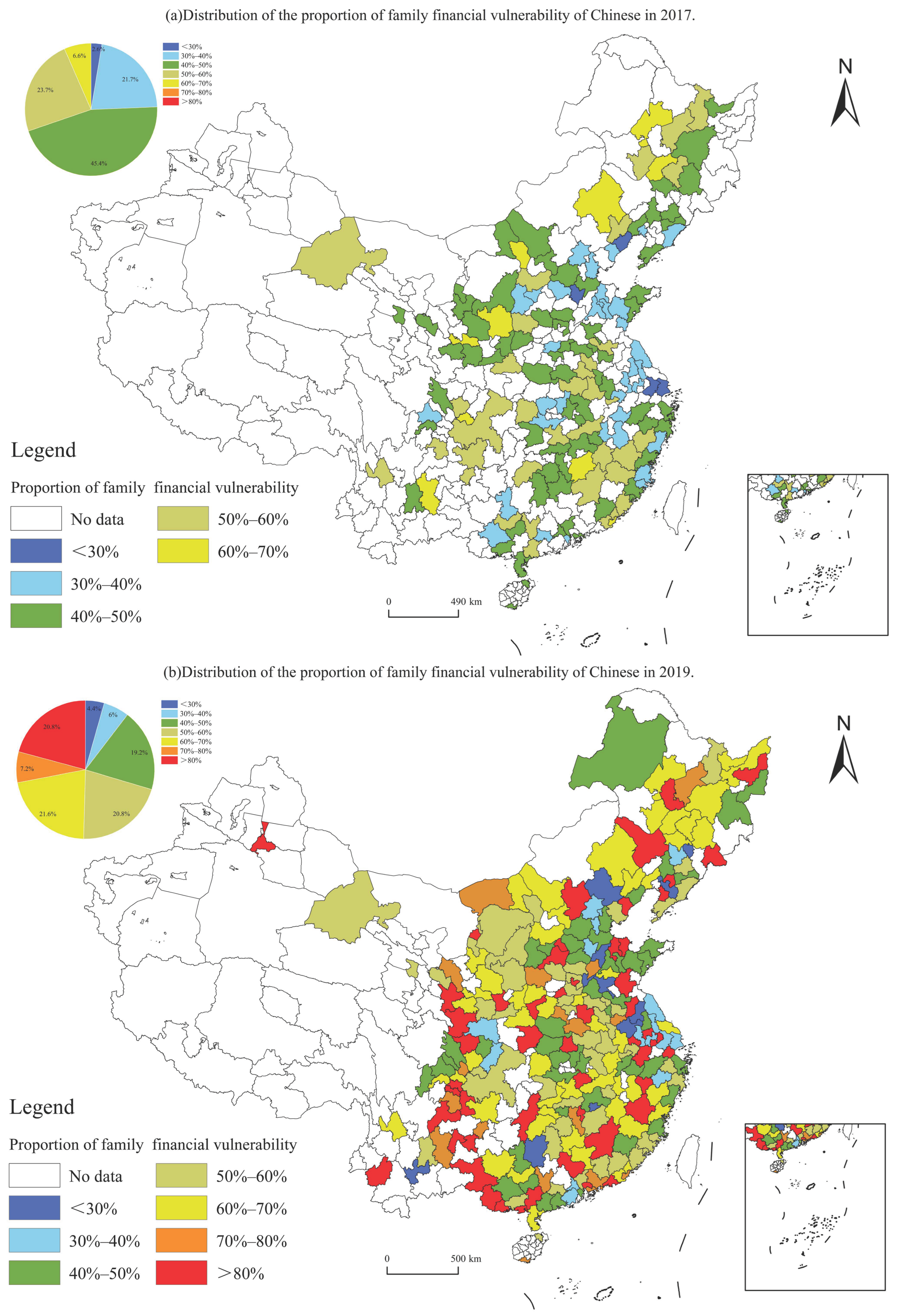
4.1. Distribution of Household Financial Vulnerability

Figure 1 shows the distribution of the proportion of financially vulnerable households in China in 2017 and 2019, based on CHFS data. In terms of spatial distribution, economically developed coastal regions and provincial capital cities in inland areas have relatively low proportions of financially vulnerable households. The majority of financially vulnerable households are located in small and medium-sized cities in central and western China. In terms of time, the proportion of financially vulnerable households in China in 2017 was mostly less than 60%, meaning that in each region, no more than 60% of households were financially vulnerable. However, these data changed significantly in 2019. Overall, more than 63% of Chinese households were financially vulnerable in 2019, and about 20.8% of regions had over 80% of households with financial vulnerability. This not only confirms the findings of Jiang and Liu [60], who used 2015 CHFS data to calculate that around 49.8% of Chinese households were financially vulnerable but also highlights the rapid increase in household financial vulnerability in China. Studying household financial vulnerability in emerging market countries such as China is crucial for promoting the sustainable development of households and the stability of national financial systems in these countries.

4.2. Performance Evaluation of Different ML Models

Table 2. Revaluation on the prediction of different ML models.

Models	(1) ${\mathit{R}}_{\mathit{I}\mathit{s}}^2$	(2) ${\mathit{R}}_{\mathit{o}\mathit{o}\mathit{s}}^2$	(3) $\mathit{E}\mathit{V}{\mathit{S}}_{\mathit{o}\mathit{o}\mathit{s}}$	(4) $\mathit{M}\mathit{S}{\mathit{E}}_{\mathit{o}\mathit{o}\mathit{s}}$	(5) $\mathit{M}\mathit{A}{\mathit{E}}_{\mathit{o}\mathit{o}\mathit{s}}$	(6) $\mathit{M}\mathit{e}\mathit{d}\mathit{A}{\mathit{E}}_{\mathit{o}\mathit{o}\mathit{s}}$
MLR	0.0778	0.0774	0.0774	0.0733	0.2599	0.2588
LASSO	0.0719	0.0628	0.0632	0.0749	0.2659	0.2658
DT	0.1998	0.1708	0.1708	0.0659	0.2304	0.2261
RF	0.2820	0.1999	0.2003	0.0640	0.2279	0.2159
GBDT	0.2394	0.2044	0.2045	0.0632	0.2272	0.2182
AdaBoost	0.1688	0.1667	0.1670	0.0666	0.2391	0.2440
XGBoost	0.2390	0.2057	0.2057	0.0631	0.2259	0.2157

presents the performance of the models for predicting household financial vulnerability based on different ML methods. First, the in-sample goodness of fit $R_{Is}^2$, out-of-sample goodness of fit $R_{oos}^2$, and out-of-sample explainable variance $EV{S}_{oos}$ are applied to evaluate the in-sample fitting performance in the training set and their out-of-sample generalization ability in the test set of seven types of ML models.

The results in column (1) of Table 2 show that the in-sample goodness of fit of LASSO regression in penalized regression is lower than that of multiple linear regression (MLR), while the in-sample goodness of fit of decision trees, random forests, GBDT, AdaBoost, and XGBoost is significantly higher than that of multiple linear regression. Among them, the random forest has the highest in-sample goodness of fit, indicating that ensemble learning methods represented by random forests, can achieve higher in-sample fitting performance than linear methods can. In terms of out-of-sample predictive ability, XGBoost has the highest out-of-sample goodness of fit and explainable variance, followed by GBDT. Compared to multiple linear regression, the out of sample goodness of fit values of Random Forest, GBDT and XGBoost improves by 162.15%, 164.08% and 165.76%, respectively. This study comprehensively utilizes out-of-sample mean squared error, out-of-sample mean absolute error, and out-of-sample absolute median error to evaluate the predictive accuracy of the model under different methods. The results show that ensemble learning methods have lower mean squared errors in out-of-sample prediction. Compared with those of multiple linear regression, the out-of-sample mean squared errors are reduced by 12.69%, 13.78%, and 13.92% when random forests, GBDT, and XGBoost are used, respectively. The average absolute errors and the absolute median errors of these three methods are also lower than those of multiple linear regression. In summary, ensemble learning methods are able to flexibly use more appropriate functions to fit the data, thus constructing a more effective and more accurate model for predicting household financial vulnerability.

The reason why ensemble learning methods outperform multiple linear regression models in prediction is that the influencing factors of household financial vulnerability are highly complex. Traditional multiple linear regression models have difficulty capturing the interactions between feature variables and the nonlinear relationships between feature variables and the response variable, leading to lower in-sample goodness of fit and weak out-of-sample generalization ability with larger errors. Whereas ensemble learning directly trains models based on the datasets and does not preset any model structure, making it more practicable to analyze the various nonlinear relationships in the model. Given that random forests and XGBoost all show significant advantages in predicting household financial vulnerability, this study further explores the disparity in the effect of different feature variables on the prediction performance of household financial vulnerability using these ensemble learning algorithms.

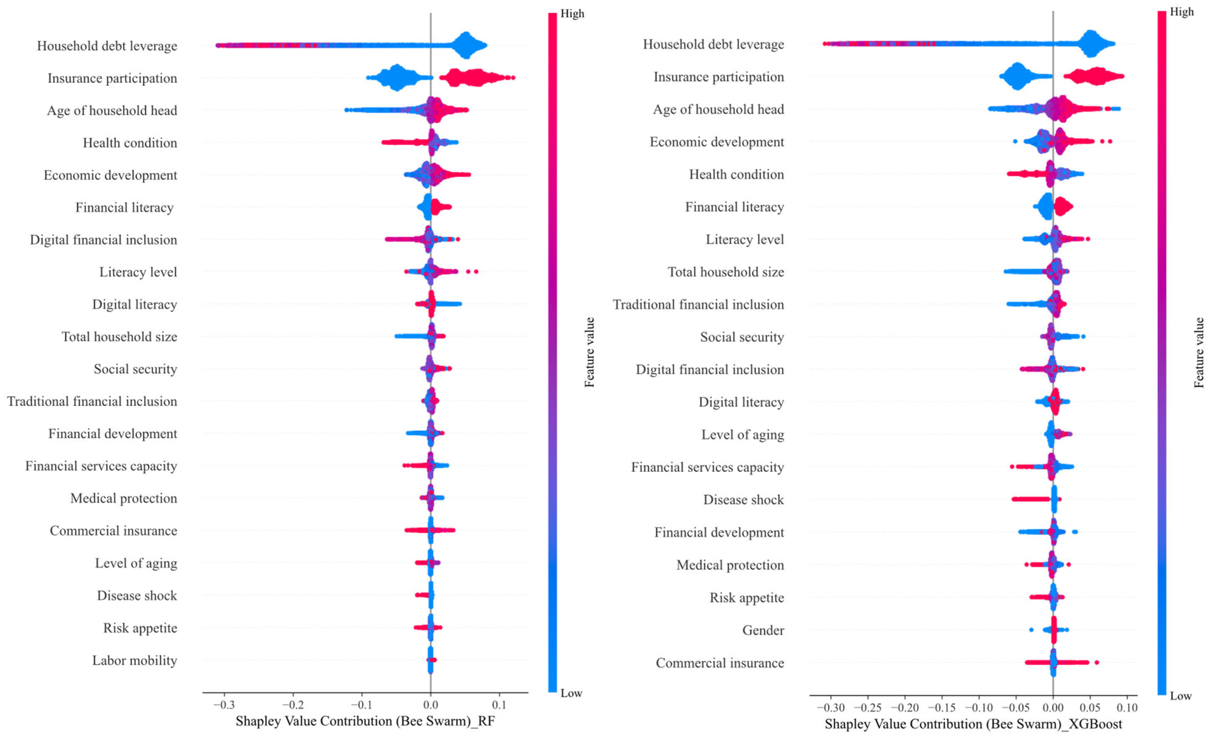
4.3. Weight Rankings of Different Feature Variables

Owing to the complexity of ensemble learning models, their predictive results are often not as intuitively interpretable as those of single learners. To uncover the underlying economic significance of ensemble learning models to examine the differences between various feature variables in measuring household financial vulnerability, this study, utilizing the SHAP method, compares the predictive effectiveness of different feature variables on household financial vulnerability.

Table 3. Importance ranking of characteristic variables based on SHAP value method.

Rank	RF		XGBoost
	Variables	SHAP	Variables	SHAP
1	Household debt leverage	0.0793	Household debt leverage	0.0804
2	Insurance participation	0.0531	Insurance participation	0.0501
3	Age of household head	0.0145	Age of household head	0.0190
4	Health condition	0.0096	Health condition	0.0124
5	Economic development	0.0081	Economic development	0.0115
6	Literacy level	0.0067	Financial literacy	0.0107
7	Financial literacy	0.0062	Literacy level	0.0080
8	Digital financial inclusion	0.0054	Total household size	0.0065
9	Social security	0.0043	Digital financial inclusion	0.0060
10	Digital literacy	0.0035	Traditional financial inclusion	0.0052

presents the top ten feature importance rankings in the two ensemble learning methods: random forest and XGBoost. The results of all methods indicate that household debt leverage, a financial characteristic, has the best forecast performance on household financial vulnerability in China, and the SHAP value for household debt leverage is 8.04% according to the XGBoost method. Additionally, the feature weight rankings validate previous research findings that household debt leverage ratio has a significant impact on financial vulnerability [61]. Meanwhile, these rankings also show that although variables such as marital status and family labor mobility influence household financial vulnerability to some extent, their significance is relatively lower, so their predictive ability for household financial vulnerability is limited.

Figure 2 presents the SHAP Bee Swarm plots generated by random forest and XGBoost. The horizontal axis in the figure represents the SHAP values generated by the corresponding model, that is, the significance of feature variables on household financial vulnerability. The vertical axis represents all feature variables. For a particular variable, color indicates the magnitude of its value, and red represents a high feature value, blue represents a low feature value.

For the three feature variables of household debt leverage, family size, and aging level, the red samples of the feature values are concentrated on the left side, while the blue samples are mostly on the right side, which indicates that the SHAP values of these three feature variables are generally negative. An increase in the household debt leverage ratio and in household size, and a higher aging level reduce the household financial margin against unexpected shocks, raising the household financial vulnerability. Among the feature variables impacting household financial vulnerability, the left-side feature values of the age of the household head, total commercial insurance expenditure in households, economic development, financial service capacity, medical care and social security are relatively low, while the right-side feature values are relatively high. This indicates that the SHAP values of the above feature variables are mainly positive. As the age of the household head and total commercial insurance expenditure increase, and regional distinctions such as economic development improve, the financial margins of households rise accordingly, thereby reducing household financial vulnerability.

For the characteristics of the household head such as physical conditions, financial literacy, and risk preference, as well as regional distinctions such as conventional inclusive finance and digital inclusive finance, their SHAP values are relatively distributed evenly, without an obviously positive or negative impact. This indicates that among the feature variables impacting household financial vulnerability, there may exist complex correlations such as nonlinear interactions between feature variables and the response variable. These feature variables have multi-dimensional impacts on household financial vulnerability and further examination is required.

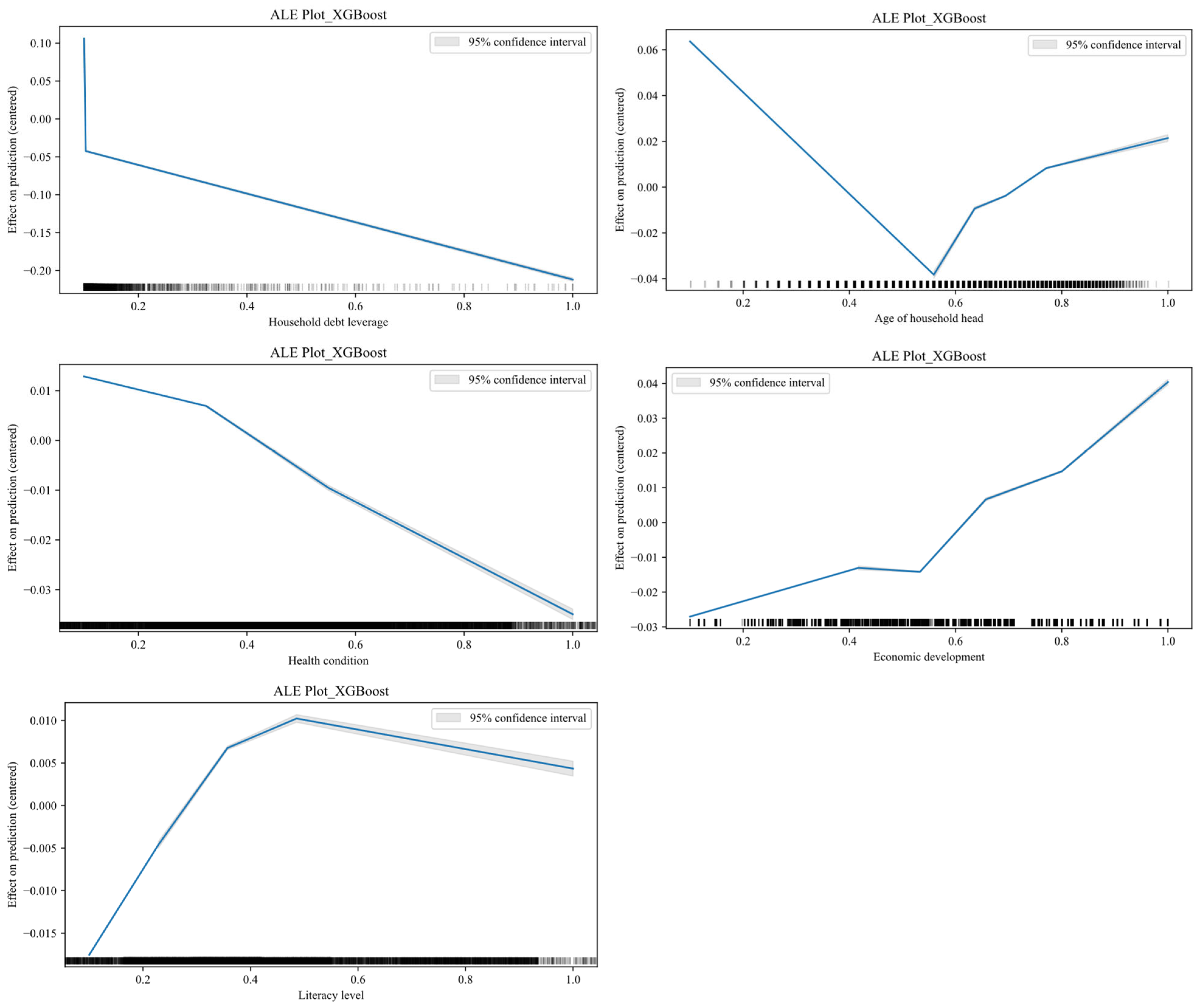
4.4. Visual Analysis of Local Effects of Major Variables

This study uses the Accumulated Local Effects (ALE) plot to analyze the specific predictive pattern of each variable on household financial vulnerability. Considering that insurance participation and financial literacy are binary variables, this study incorporates education level, which ranks high in feature weight, into the analysis, and generates ALE plots for features of household debt leverage, age of household head, health conditions, economic development, and literacy level, where the vertical axis represents the size of the accumulated local effect indicating the average impact of value changes on the model’s predictive output, and the slope of the blue solid line represents the marginal effect of feature variables. The dashed line in the ALE plot represents the marginal distribution of Monte Carlo samples, reflecting the uncertainty in the model’s predictions upon specific feature values. The closer the dashed line is to the solid line, the more consistent the predictions are for the Monte Carlo samples near that feature value, indicating lower model uncertainty. Figure 3 presents the ALE plots for five feature variables—household debt leverage, age of household head, health conditions, economic development, and literacy level—based XGBoost.

As shown in Figure 3, as the household debt leverage ratio increases, the household financial margin against unanticipated shocks shrinks correspondingly, signifying a rise in household financial vulnerability. The household debt burden may cause a leverage effect, where indebted households often need more debt to meet current consumption and repay previous debts [62], thus forming debt leverage. Households with high debt leverage are weak in cushioning financial shocks and addressing income decrease if income fluctuates, which will break the household financial balance and increase the debt ratio in family assets. In the end, household net asset decreases and the ability to resist risk weakens as well. Additionally, from the perspective of financial market conductibility, households with high debt leverage are more susceptible to external factors such as interest rates and housing prices, so their financial risk exposure may be amplified. Under the financial stress, households are prone to make suboptimal financial decisions, such as liquidating assets too soon or reducing investment and spending, thereby household financial vulnerability being raised.

As the age of the household head increases, the household financial margin against unanticipated shocks tends to decline, so financial vulnerability increases. However, when the age of the household head continues to rise, the margin begins to increase, and household financial vulnerability decreases. There is an inverted “V”-shaped relation between the age of household head and household financial vulnerability. According to the life cycle theory, generally, households balance their consumption and savings throughout their life cycle. In the early adult stage, households have lower incomes but expect future income growth. Therefore, even if the current affordability is overdrafted, households may still maintain high debt leverage to support investments such as education and house purchases, which increases household financial vulnerability [63]. As age increases, household income gradually rises, so the debt level decreases, and accumulating wealth reduces financial vulnerability gradually. Moreover, from the perspective of financial literacy, younger household heads often lack sufficient financial awareness and experience, which leads to biased financial decisions, further exacerbating household financial vulnerability. As the household head grows sophisticated and accumulates experience, his financial literacy and asset management improve, effectively optimizing the household financial structure and reducing financial vulnerability.

Different from other feature variables, the x-axis of the ALE graph for health condition in this study represents gradually declining physical health. As health deteriorates, household financial margin initially decreases slowly, but after a certain threshold it drops rapidly, and the household financial vulnerability rises at an accelerating rate. This can be regarded as an integrated phenomenon of accumulated risk and threshold effects. Even if the household head is still in average physical condition, his declining health not only increases the instability of household income, but also consumes family wealth due to the rising medical expenses, thus increasing financial vulnerability slowly of households. If the household head is in poor condition, apart from his inability to work, it also leads to a decrease in family income for the care giving burden. In addition, the huge medical expenses will consume household financial reserves, resulting in a rapid increase in financial vulnerability.

As shown in Figure 3, if local economy is underdeveloped, the household financial margin against unanticipated shocks decreases as economy develops, and household financial vulnerability rises. However, when economic development exceeds a certain threshold, financial vulnerability begins to decrease with further economic growth. This phenomenon can be explained by the differences in household income volatility, attitudes towards consumption and savings, and the regional financial system across various stages of economic development. In the economically underdeveloped stage, household income is dependent on undiversified sources, bearing weak anti-risk capacity and conservative consumption ideas, and local financial services are in low popularization. As the economy develops, household income becomes more volatile and residents tend to expand their consumption, which reduces their financial margin. Meanwhile, the developing local financial system makes it more accessible for households to purchase financial products with high yield but also high risk. Thus, the financial vulnerability of households increases. As the local economy reaches a certain threshold, household income surges significantly and income sources diversify, so households can realize a high savings rate after covering their consumption, thus enhancing their anti-risk capacity. Furthermore, the developed local financial system and the highly popularized financial services enable households to disperse and control the possible risks in a financial way, so the growth rate of household financial vulnerability tends to slow down.

As the literacy level of the household head improves, household financial margin against unanticipated shocks increases, and household financial vulnerability shows a downward trend. But after a certain threshold, vulnerability becomes relatively stable, and no significant upward or downward trend is observed. The highly educated possess more stable jobs with higher pay, and they can discern and assess potential financial risks more precisely and mitigate them through precautionary measures such as insurance. In addition, they have broader social networks and more access to social resources. Therefore, compared with those with lower education, they are more resilient financially in the face of income loss [64]. However, if the household head has obtained education highly enough, the marginal effect of further education on financial decision-making diminishes, and the mitigation of household financial vulnerability is no longer significant.

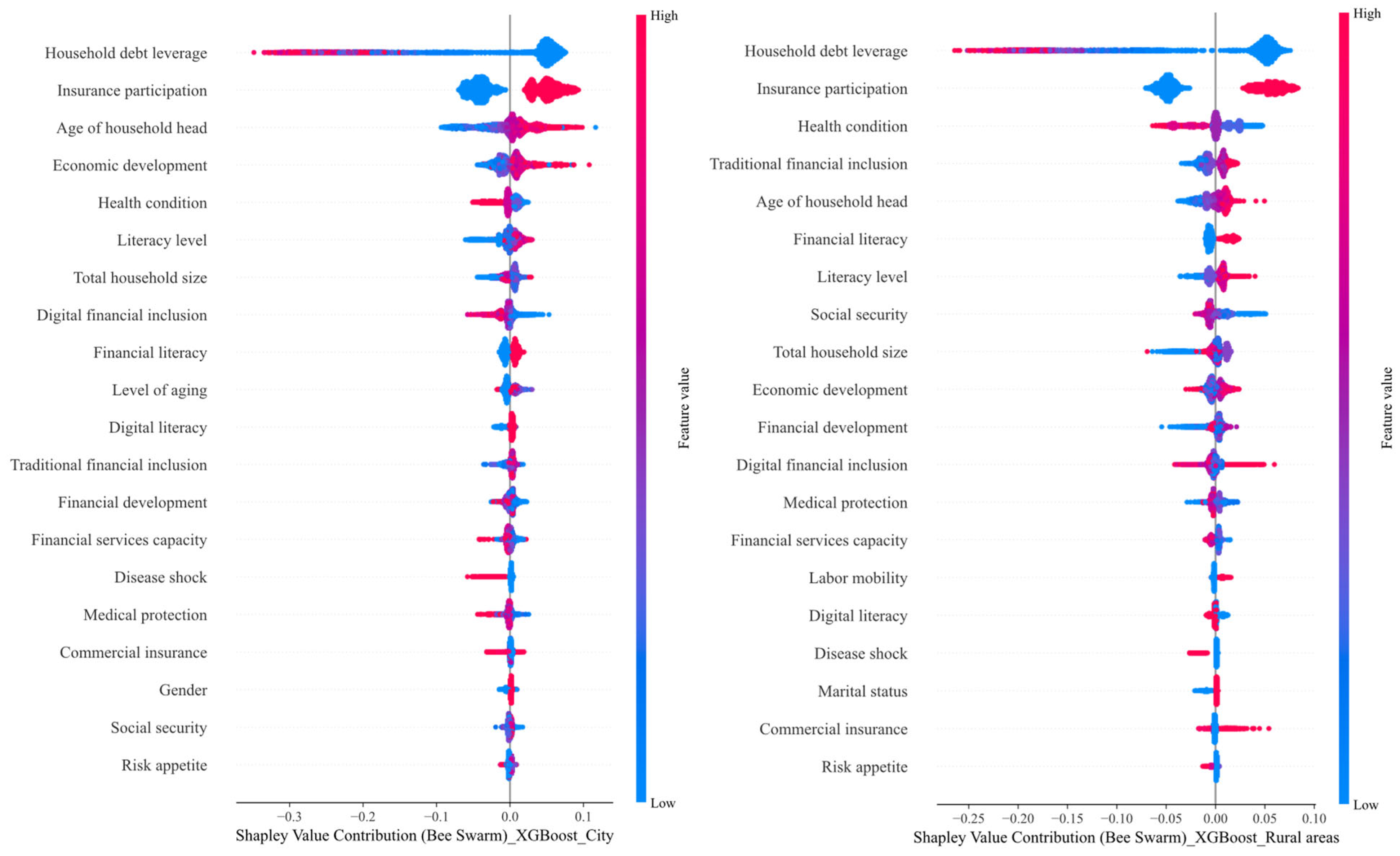
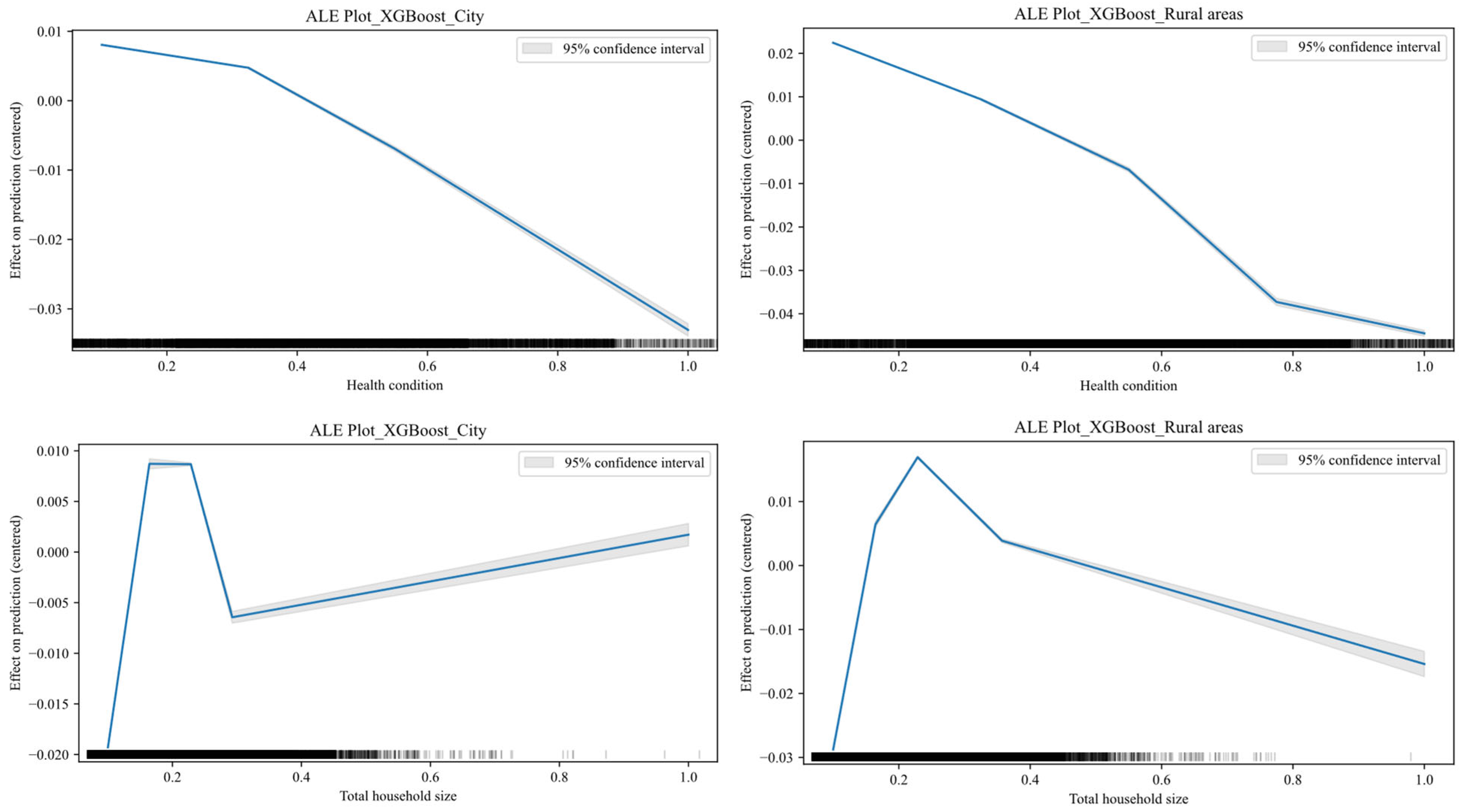
4.5. Analysis on Heterogeneity in Financial Vulnerability Between Urban and Rural Areas

China’s urban-rural dual structure results in a structural mismatch of financial resources between urban and rural areas. Compared with urban areas, finance in rural areas is relatively underdeveloped, and the effective financial demands of rural households cannot be fully met [65,66]. Therefore, financial vulnerability in China may vary in extent between rural and urban households. In order to explore the differences in factors that influence household financial vulnerability between urban and rural households in China, this study divides the samples into urban and rural ones according to their residential information for comparative research.

Table 4. Importance ranking of household characteristic variables in urban and rural areas.

Rank	Urban Family		Rural Family
	Variables	SHAP	Variables	SHAP
1	Household debt leverage	0.0825	Household debt leverage	0.0730
2	Insurance participation	0.0466	Insurance participation	0.0538
3	Age of household head	0.0229	Health condition	0.0159
4	Economic development	0.0127	Total household size	0.0094
5	Literacy level	0.0083	Age of household head	0.0093
6	Health condition	0.0082	Financial literacy	0.0093
7	Financial literacy	0.0078	Economic development	0.0089
8	Digital financial inclusion	0.0068	Social security	0.0087
9	Total household size	0.0067	Literacy level	0.0074
10	Level of aging	0.0067	Digital financial inclusion	0.0061

and Figure 4 present the feature importance rankings and SHAP bee swarm plots of the urban and rural household subsamples, respectively, based on the XGBoost method. The results show that household debt leverage and insurance participation are the most significant feature variables in predicting household financial vulnerability both in urban and rural household samples. In addition, the heterogeneity analysis reveals that, in addition to the aforementioned features, the age of the household head is the most significant feature impacting urban household financial vulnerability, while for rural households, the health condition is the most significant. Furthermore, in the case of urban households, the aging level ranks among the top ten variables influencing financial vulnerability, where an increase in the proportion of the old in households leads to greater household financial vulnerability. For rural households, social security is the key variable, as improvement in rural social security reduces financial vulnerability significantly.

This study further analyses the heterogeneity of health condition and household size features in measuring financial vulnerability in urban and rural households. By comparing the ALE graphs (Figure 5) for health conditions between urban and rural households, it can be observed that for urban households, as physical health deteriorates, their financial margin slowly drops at first, followed by a rapid decline, meaning that household financial vulnerability first increases slowly and then increases rapidly. In contrast, the rate at which the financial vulnerability upon deteriorating physical health in rural households increases is notably higher than in urban households, and the impact is more significant. The root cause lies in the reality that rural households rely more heavily on the health of the household head. In specific, rural household income is mainly dependent on the physical labor of the household head, so a deterioration in the household head’s health directly reduces household income. Moreover, insurance and market mechanisms in rural areas are not developed enough to mitigate this risk. In addition, medical resources are relatively scarce in rural areas, so the cost of medical treatment poses a more severe threat to family finances. Therefore, a deterioration in the health of household heads is a multiple blow from several aspects to rural households, not only impairing their earning power but also imposing additional financial burdens on them. Whereas, in urban areas, the impact is mitigated to some extent by improved social security system and diversified income sources. In the end, it gives rise to disparity in financial vulnerability between urban and rural households.

As is observed in the ALE plot of urban and rural household size, expanding family size causes their financial margin against unanticipated shocks of both urban and rural households to rise and then fall, initially. However, when it reaches a certain threshold, the impact of family size on financial vulnerability is opposite in urban and rural households: for urban households, financial vulnerability decreases as family size increases, while for rural households, financial vulnerability increases as family size grows. The cause of this phenomenon lies in the structural disparities between urban and rural households in terms of income diversification, social security coverage, labor market distinctions, educational resources, family resource division, and the utilization of social support systems. Urban households can spread risks through diversified employment and social insurance of family members to mitigate financial vulnerability. While rural households are constrained by limited land production and employment opportunities, increasing family members may drag down per-head resources and intensify economic pressure. And insufficient social security and the limited social support system in rural areas exacerbate financial vulnerability if household size expands. This also signifies the significant differences in economic resilience and risk-bearing capacity between urban and rural households in face of changing family size.

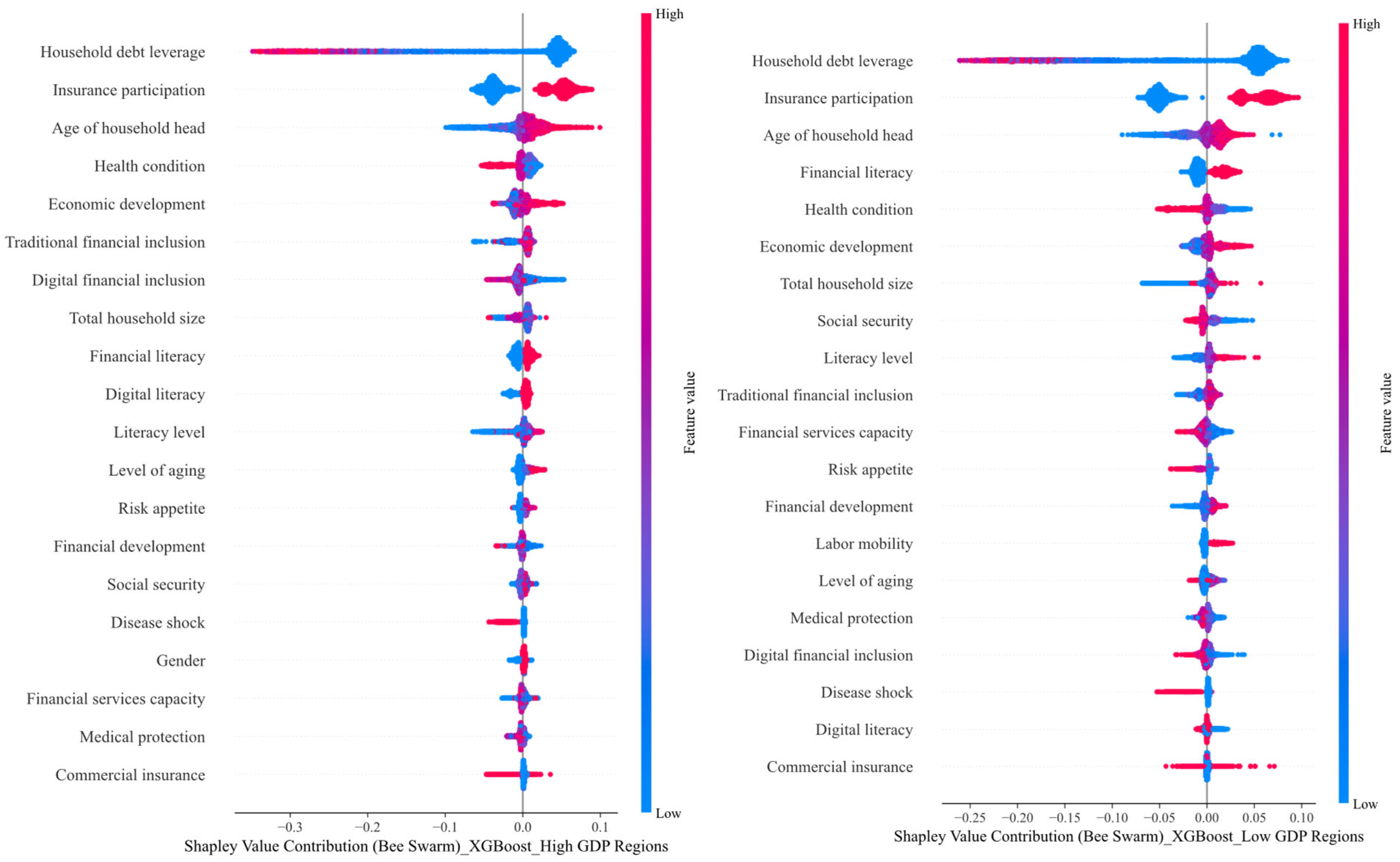
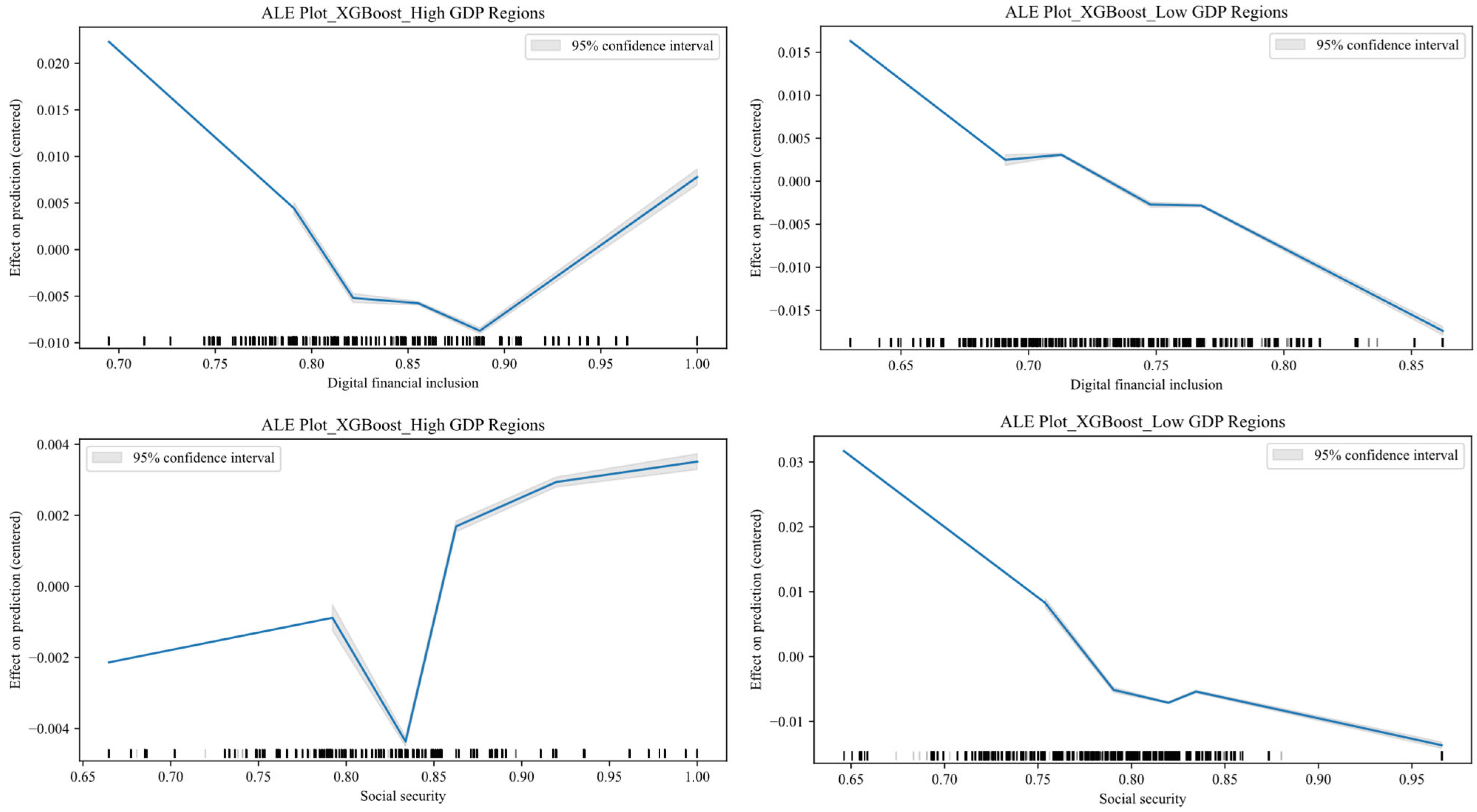
4.6. Heterogeneity Analysis of Household Financial Vulnerability Based on per Capita GDP

Developed and developing regions typically exhibit significant disparities in resident income levels, social security systems, and financial market maturity. These fundamental economic differences profoundly shape the types of risks households face, the resources available to buffer shocks, and financial behavioral patterns, thereby molding distinct characteristics of financial vulnerability and coping strategies across regions. Consequently, this study defines the top 50% of samples by per capita GDP as developed regions and the bottom 50% as developing regions. This classification aims to uncover key heterogeneities in the factors influencing household financial vulnerability across different development stages, providing a basis for formulating targeted policies for different regions.

Table 5. Importance ranking of family characteristic variables in different development levels regions.

Rank	High GDP Regions		Low GDP Regions
	Variables	SHAP	Variables	SHAP
1	Household debt leverage	0.0759	Household debt leverage	0.0799
2	Insurance participation	0.0437	Insurance participation	0.0533
3	Age of household head	0.0178	Age of household head	0.0154
4	Health condition	0.0101	Financial literacy	0.0123
5	Economic development	0.0095	Health condition	0.0111
6	Traditional financial inclusion	0.0085	Economic development	0.0085
7	Digital financial inclusion	0.0083	Total household size	0.0074
8	Total household size	0.0080	Social security	0.0073
9	Financial literacy	0.0076	Literacy level	0.0070
10	Digital literacy	0.0063	Traditional financial inclusion	0.0054

and Figure 6 present the feature importance rankings and SHAP Bee Swarm plots for the high per capita GDP and low per capita GDP sub-samples, derived using the XGBoost method. The heterogeneity analysis reveals that within the high per capita GDP group, digital financial inclusion and digital literacy occupy prominent positions among the features influencing financial vulnerability. The SHAP summary plot for high per capita GDP households indicates that higher digital literacy significantly reduces household financial vulnerability, while the direction of digital financial inclusion’s impact is less certain. Conversely, for low per capita GDP households, social security coverage and educational attainment feature within the top ten influential characteristics. The corresponding SHAP plot shows that increased educational attainment significantly lowers financial vulnerability in this group, whereas higher social security levels exhibit the opposite effect.

To probe deeper into regional differences, this study selected two features with significant yet divergent impacts on household financial vulnerability across regions—digital financial inclusion for high per capita GDP areas and social security for low per capita GDP areas—and analyzed them using ALE plots. Figure 7 demonstrates that as digital financial inclusion develops, the unexpected financial margin (a key indicator of fragility) decreases for households in both high and low per capita GDP regions, suggesting an initial rise in financial vulnerability. However, upon further advancement of digital financial inclusion, fragility continues to rise in low per capita GDP regions but begins to decline in high per capita GDP regions. This pattern resonates with the findings by Waliszewski et al. [67] on the “double-edged sword” effect of LendTech. They argue that while non-bank lending sectors can provide credit services supplementing banks, they also heighten the risk of over-indebtedness. The proliferation of non-bank lending observed here is emblematic of digital financial inclusion development in this study. Once digital financial inclusion matures, supported by stronger market regulation, enhanced financial literacy, and better digital infrastructure, households in high per capita GDP regions develop improved risk management capabilities. This enables them to effectively utilize both bank and non-bank channels for household fund circulation, ultimately reducing financial vulnerability. Conversely, for households in low per capita GDP regions, where financial literacy is generally lower, maturing digital financial inclusion increases the risk of over-indebtedness, deepens household debt risks, and consequently leads to persistently elevated fragility.

The ALE plot for social security indicates that while its relationship with financial vulnerability in high per capita GDP regions is nonlinear, an overall increase in social security coverage reduces fragility. In stark contrast, for low per capita GDP regions, higher social security levels correlate with a consistent rise in household financial vulnerability. In high per capita GDP regions, robust social security systems effectively buffer external shocks, smooth household consumption, and free up resources for productive investment and risk management, thereby systemically lowering vulnerability. In low per capita GDP regions, constrained fiscal capacity results in narrow coverage, low benefit levels, and inefficient social security systems. This inadequate protection can crowd out informal household mutual aid networks and private savings. Many households face increased burdens from inappropriate financing methods, leading to an erosion of actual risk-buffering capacity and consequently higher financial vulnerability.

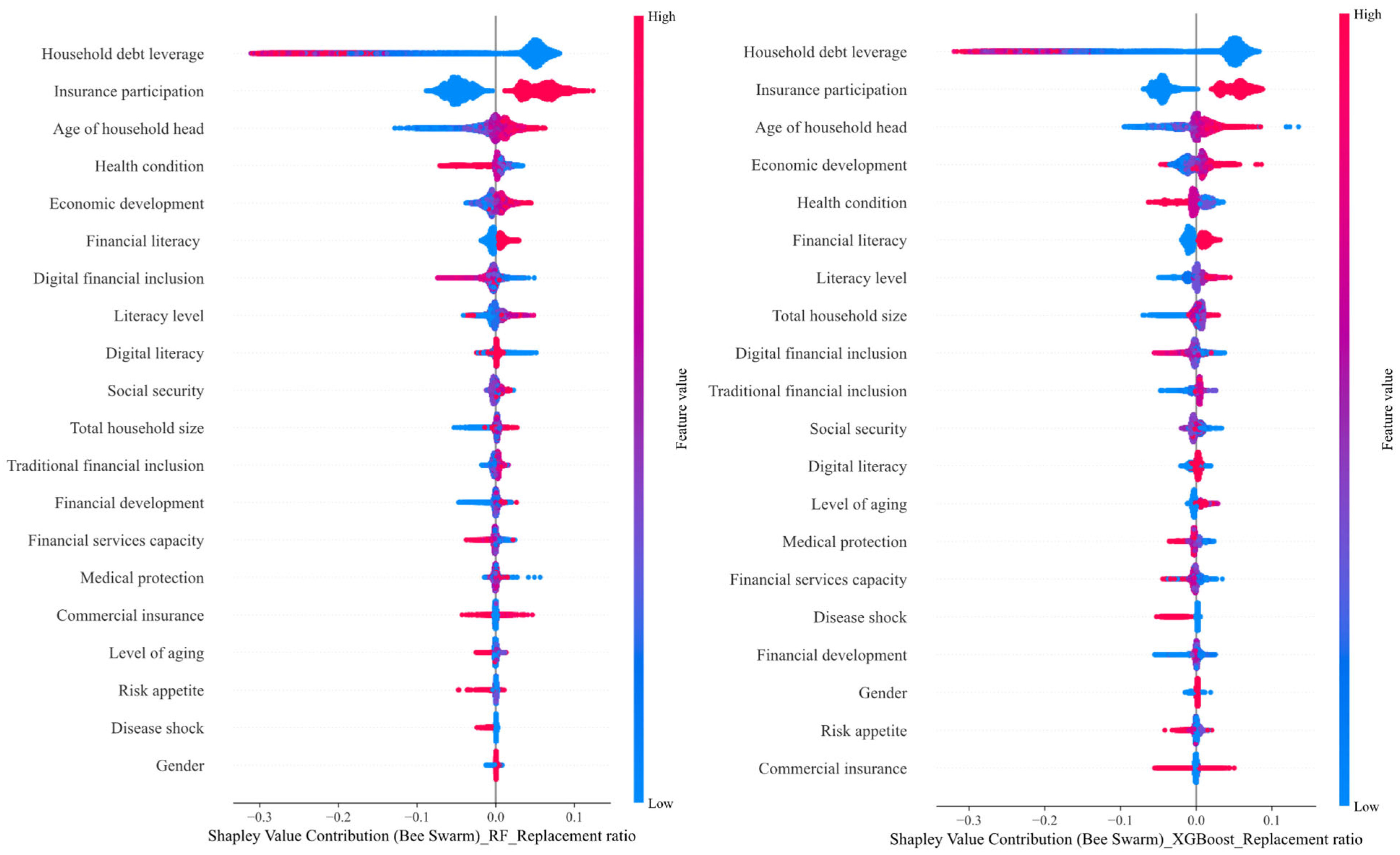
4.7. Robustness Test

This study employs household financial margin against unanticipated shocks as the response variable in the main test. In order to examine the applicability of the research conclusions, this study refers to Chen et al. [68], who measure household financial vulnerability through accumulated household financial risk and risk resistance capacity. In their study, household marginal finance $F{M}_{it}=Y_{it}-L{C}_{it}$ and family financial capacity $C{F}_{it}=(Y_{it}+L{A}_{it})/L{C}_{it}$ are applied as substitute response variables. If the household marginal finance $F{M}_{it}\ge 0$, the household is considered to bear no financial vulnerability, with a value of −1; if $F{M}_{it}<0 \mathit{and} C{F}_{it}\ge 1$, the household is considered to experience low financial vulnerability, with a value of 0; and if $F{M}_{it}<0 \mathit{and} C{F}_{it}<1$, the household is considered to exhibit high financial vulnerability, with a value of 1. The results in Panel A of

Table 6. Robustness test of model prediction performance.

Models	(1) ${\mathit{R}}_{\mathit{I}\mathit{s}}^2$	(2) ${\mathit{R}}_{\mathit{o}\mathit{o}\mathit{s}}^2$	(3) $\mathit{E}\mathit{V}{\mathit{S}}_{\mathit{o}\mathit{o}\mathit{s}}$	(4) $\mathit{M}\mathit{S}{\mathit{E}}_{\mathit{o}\mathit{o}\mathit{s}}$	(5) $\mathit{M}\mathit{A}{\mathit{E}}_{\mathit{o}\mathit{o}\mathit{s}}$	(6) $\mathit{M}\mathit{e}\mathit{d}\mathit{A}{\mathit{E}}_{\mathit{o}\mathit{o}\mathit{s}}$
Panel A Change response variable
MLR	0.0294	0.0297	0.0297	0.7413	0.7792	0.8534
LASSO	0.0288	0.0263	0.0263	0.7517	0.7882	0.8625
DT	0.0621	0.0475	0.0475	0.7277	0.7713	0.8167
RF	0.1662	0.0565	0.0570	0.7279	0.7731	0.7843
GBDT	0.1069	0.0702	0.0702	0.7104	0.7626	0.7987
AdaBoost	0.0346	0.0313	0.0315	0.7473	0.7865	0.8802
XGBoost	0.1009	0.0716	0.0716	0.7093	0.7611	0.7999
Panel B Randomly divide the datasets into a training set and a test set in a 7:3 ratio
MLR	0.0776	0.0771	0.0772	0.0734	0.2600	0.2583
LASSO	0.0740	0.0628	0.0628	0.0749	0.2657	0.2652
DT	0.1985	0.1774	0.1775	0.0655	0.2299	0.2225
RF	0.2600	0.1937	0.1938	0.0644	0.2291	0.2174
GBDT	0.2393	0.2096	0.2097	0.0629	0.2262	0.2161
AdaBoost	0.1703	0.1623	0.1623	0.0669	0.2406	0.2446
XGBoost	0.2456	0.2114	0.2114	0.0628	0.2247	0.2139

show that the conclusions after replacing the response variable are consistent with those of previous main analysis.

To exclude possible output error due to single sample division, this study randomly divides the datasets into training and test sets anew with a 7:3 ratio, and tests if new sample intervals fit the model, with the results shown in Panel B of Table 6 and Figure 8. With newly divided datasets, the predictive ability on household financial vulnerability of ensemble learning methods (i.e., Random Forest, GBDT, and XGBoost) remains significantly greater than that of multiple linear regression. The ranking of feature variable importance based on random forest and XGBoost is consistent with the main test. Therefore, the conclusions of this study are further validated by robust tests.

5. Conclusions and Recommendations

This study, conducted on the basis of the 2017 and 2019 China Household Finance Survey data, represents the distribution of financially vulnerable households across various regions of China. By machine learning (ML), SHapley Additive exPlanations (SHAP), and accumulative local effects (ALE) plot, this paper analyzes the feature variables influencing household financial vulnerability and identifies the most significant one, and summarizes the specific predictive patterns of each variable. Simultaneously, this study conducted a comparative analysis of household financial vulnerability between urban and rural Chinese households, as well as between high and low per capita GDP regions.

Compared with previous studies on household financial vulnerability that examine only a few features under specific theoretical frameworks, this research compares various predictive features impacting household financial vulnerability comprehensively through the ML and SHAP methods. The results show that the proportion of financially vulnerable households is lower in economically developed coastal regions and inland provincial capitals, while the majority of financially vulnerable households are located in medium-sized cities in central and western part of China. In 2019, more than 63% of Chinese households were financially vulnerable, and regions in which the proportion of financially vulnerable households was over 80% covered 20.8% of China. The SHAP method reveals that the financial feature variable of household debt leverage is the most significant in predicting financial vulnerability, with a positive significance of 8.04%. The ALE plots demonstrate the nonlinear relations of household debt leverage, age of household head, health condition, regional economic development and literacy level with financial vulnerability. Heterogeneity analysis reveals that, except for household debt leverage and insurance participation, the key characteristic variables exerting the most pronounced effect on financial fragility differ between urban and rural households: household head age for urban families and physical health status for rural families. Furthermore, digital financial inclusion and social security exert distinct impacts on financial vulnerability, showing significantly stronger effects in high per capita GDP regions and low per capita GDP regions, respectively.

Against the backdrop of significantly rising household financial vulnerability rates in emerging economies, exemplified by China, the findings of this research hold substantial importance for thoroughly identifying key determinants of household financial vulnerability and advancing sustainable household development alongside financial system stability in these nations. These insights can assist government authorities in refining financial policies. Concretely, governments could establish a multi-tiered household debt relief and prevention framework. Through collaboration with financial institutions, they could formulate tiered debt relief programs encompassing measures such as debt restructuring, interest subsidies, and extended repayment periods-particularly targeting low-income and rural households. Simultaneously, governments should enhance rural health security systems and implement comprehensive family support initiatives. This includes promoting rural household health record systems and leveraging big data health analytics, developing tailored health insurance products for rural household heads. Providing premium subsidies (especially for those with chronic conditions) and implementing special medical protection plans are crucial to mitigate disease-induced poverty risks. For instance, partnerships with insurers could yield affordable critical illness coverage specifically for rural household heads. Beyond this, a suite of integrated family support policies could be introduced, including but not limited to: Additional educational grants for large rural families to ensure children’s education remains unaffected by financial constraints; Family-size-adaptive tax incentives to alleviate economic burdens on large households; Family-size-linked social security measures, such as dedicated large-family relief funds to address sudden economic hardships.

However, in this study, although the factors influencing household financial vulnerability in China have been discerned by ML, and the predictive ability and influencing mechanism of each feature are presented by SHAP values and ALE plots, which comes to conclusions never made in previous studies through explanatory modeling, this study cannot test the causality within these conclusions as other research focusing on the predictive ability cannot either. Secondly, although this paper identified 27 characteristics that affect household financial vulnerability, due to the limitations of the dataset, not all characteristic variables were included. It is expected that future research integrates ML methods with causal inference frameworks further. Hence, a model of analyzing counterfactual combinations can be constructed by Difference-in-Differences (DID) on ML to investigate the causal relations between feature variables and response variable, and select other datasets, incorporating more characteristic variables that affect household financial vulnerability into the analysis, thereby deepening the understanding of the factors associated with household financial vulnerability.

References

1. Fernández-López, S.; Álvarez-Espiño, M.; Rey-Ares, L. Financial vulnerability of low-income households: Review of scopus and wos journals and future research agenda. Appl. Econom. Int. Dev. 2024, 24, 153–180. [Google Scholar]
2. Leandro, J.C.; Botelho, D. Consumer over-indebtedness: A review and future research agenda. J. Bus. Res. 2022, 145, 535–551. [Google Scholar] [CrossRef]
3. Acharya, V.; Bhadury, S.; Surti, J. Financial Vulnerability and Risks to Growth in Emerging Markets (No. w27411); National Bureau of Economic Research: Cambridge, UK, 2020; Available online: https://www.nber.org/papers/w27411 (accessed on 23 April 2025).
4. The World Bank. World Development Report 2022: Finance for an Equitable Recovery; The World Bank: Washington, DC, USA, 2022. [Google Scholar]
5. Waxman, A.; Liang, Y.; Li, S.; Barwick, P.J.; Zhao, M. Tightening belts to buy a home: Consumption responses to rising housing prices in urban China. J. Urban Econ. 2020, 115, 103190. [Google Scholar] [CrossRef]
6. Wu, F.; Chen, J.; Pan, F.; Gallent, N.; Zhang, F. Assetization: The Chinese path to housing financialization. Ann. Am. Assoc. Geogr. 2020, 110, 1483–1499. [Google Scholar] [CrossRef]
7. Rothwell, D.W.; Giordono, L.; Stawski, R.S. How much does state context matter in emergency savings? Disentangling the individual and contextual contributions of the financial capability constructs. J. Fam. Econ. Issues 2022, 43, 703–715. [Google Scholar] [CrossRef]
8. Ali, L.; Khan, M.K.N.; Ahmad, H. Financial vulnerability of Pakistani household. J. Fam. Econ. Issues 2020, 41, 572–590. [Google Scholar] [CrossRef]
9. Bettocchi, A.; Giarda, E.; Moriconi, C.; Orsini, F.; Romeo, R. Assessing and predicting financial vulnerability of Italian households: A micro-macro approach. Empirica 2018, 45, 587–605. [Google Scholar] [CrossRef]
10. Gao, H. The effects of financial spatial structure on household financial vulnerability: Evidence from China. PLoS ONE 2024, 19, e0313189. [Google Scholar] [CrossRef]
11. Pan, H.; Yao, L.; Zhang, C.; Zhang, Y.; Gao, Y. Research on financial poverty alleviation aid for increasing the incomes of low-income Chinese farmers. Sustainability 2024, 16, 1057. [Google Scholar] [CrossRef]
12. Lee, C.C.; Jiang, L.; Wen, H. Two aspects of digitalization affecting financial asset allocation: Evidence from China. Emerg. Mark. Financ. Trade 2024, 60, 631–649. [Google Scholar] [CrossRef]
13. Batty, M.; Gibbs, C.; Ippolito, B. Health insurance, medical debt, and financial well-being. Health Econ. 2022, 31, 689–728. [Google Scholar] [CrossRef]
14. Yue, P.; Korkmaz, A.G.; Yin, Z.; Zhou, H. The rise of digital finance: Financial inclusion or debt trap? Finance Res. Lett. 2022, 47, 102604. [Google Scholar] [CrossRef]
15. Ramli, Z.; Nyirop, H.B.A.; Sum, S.M.; Awang, A.H. The impact of financial shock, behavior, and knowledge on the financial vulnerability of single youth. Sustainability 2022, 14, 4836. [Google Scholar] [CrossRef]
16. Zhang, Y.; Wu, Q.; Zhang, T.; Yang, L. Vulnerability and fraud: Evidence from the COVID-19 pandemic. Humanit. Soc. Sci. Commun. 2022, 9, 424. [Google Scholar] [CrossRef]
17. Athey, S. The Impact of Machine Learning on Economics. In The Economics of Artificial Intelligence: An Agenda; University of Chicago Press: Chicago, IL, USA, 2018; pp. 507–552. [Google Scholar]
18. Mullainathan, S.; Spiess, J. Machine learning: An applied econometric approach. J. Econ. Perspect. 2017, 31, 87–106. [Google Scholar] [CrossRef]
19. Minsky, H.P. The financial instability hypothesis: An interpretation of keynes and an alternative to “standard” theory. Challenge 1977, 20, 20–27. [Google Scholar] [CrossRef]
20. Lusardi, A.; Schneider, D.; Tufano, P. Financially Fragile Households: Evidence and Implications (No. w17072); National Bureau of Economic Research: Cambridge, UK, 2011. [Google Scholar]
21. Jappelli, T.; Pagano, M.; Di Maggio, M. Households’ indebtedness and financial vulnerability. J. Financ. Manag. Mark. Inst. 2013, 1, 23–46. [Google Scholar]
22. Lusardi, A.; Tufano, P. Debt literacy, financial experiences, and overindebtedness. J. Pension Econ. Financ. 2015, 14, 332–368. [Google Scholar] [CrossRef]
23. Dang, C.; Chen, X.; Yu, S.; Chen, R.; Yang, Y. Credit ratings of Chinese households using factor scores and K-means clustering method. Int. Rev. Econ. Financ. 2022, 78, 309–320. [Google Scholar] [CrossRef]
24. Noerhidajati, S.; Purwoko, A.B.; Werdaningtyas, H.; Kamil, A.I.; Dartanto, T. Household financial vulnerability in Indonesia: Measurement and determinants. Econ. Model. 2021, 96, 433–444. [Google Scholar] [CrossRef]
25. Kuypers, S.; Marx, I. The truly vulnerable: Integrating wealth into the measurement of poverty and social policy effectiveness. Soc. Indic. Res. 2019, 142, 131–147. [Google Scholar] [CrossRef]
26. Chen, H.L.; Hsu, Y.L.; Lu, C.Y. Revisiting financial vulnerability during the COVID-19 pandemic: Evidence from Taiwan. J. Behav. Exp. Financ. 2024, 44, 100993. [Google Scholar] [CrossRef]
27. Chhatwani, M.; Mishra, S.K. financial vulnerability and financial optimism linkage during COVID-19: Does financial literacy matter? J. Behav. Exp. Econ. 2021, 94, 101751. [Google Scholar] [CrossRef] [PubMed]
28. Kleimeier, S.; Hoffmann, A.O.I.; Broihanne, M.H.; Plotkina, D.; Göritz, A.S. Determinants of individuals’ objective and subjective financial vulnerability during the COVID-19 pandemic. J. Bank. Financ. 2023, 153, 106881. [Google Scholar] [CrossRef]
29. Ampudia, M.; Van Vlokhoven, H.; Żochowski, D. Financial vulnerability of euro area households. J. Financ. Stab. 2016, 27, 250–262. [Google Scholar] [CrossRef]
30. Lusardi, A.; Mitchell, O.S.; Oggero, N. Debt and financial vulnerability on the verge of retirement. J. Money. Credit. Bank 2020, 52, 1005–1034. [Google Scholar] [CrossRef]
31. Daud, S.N.M.; Marzuki, A.; Ahmad, N.; Kefeli, Z. Financial vulnerability and its determinants: Survey evidence from Malaysian households. Emerg. Mark. Financ. Trade 2019, 55, 1991–2003. [Google Scholar] [CrossRef]
32. Kim, H.J.; Lee, D.; Son, J.C.; Son, M.K. Household indebtedness in Korea: Its causes and sustainability. Jpn. World Econ. 2014, 29, 59–76. [Google Scholar] [CrossRef]
33. Kim, K.T.; Xiao, J.J.; Porto, N. Financial inclusion, financial capability and financial vulnerability during COVID-19 pandemic. Int. J. Bank Mark. 2024, 42, 414–436. [Google Scholar] [CrossRef]
34. Korniotis, G.M.; Kumar, A. Do older investors make better investment decisions? Rev. Econ. Stat. 2011, 93, 244–265. [Google Scholar] [CrossRef]
35. Angrisani, M.; Burke, J.; Lusardi, A.; Mottola, G. The evolution of financial literacy over time and its predictive power for financial outcomes: Evidence from longitudinal data. J. Pension Econ. Financ. 2023, 22, 640–657. [Google Scholar] [CrossRef]
36. Hasler, A.; Lusardi, A.; Yagnik, N.; Yakoboski, P. Resilience and wellbeing in the midst of the COVID-19 pandemic: The role of financial literacy. J. Account. Public Policy 2023, 42, 107079. [Google Scholar] [CrossRef]
37. Yusof, S.A. Ethnic disparity in financial vulnerability in Malaysia. Int. J. Soc. Econ. 2019, 46, 31–46. [Google Scholar] [CrossRef]
38. Morudu, P.; Kollamparambil, U. Health shocks, medical insurance and household vulnerability: Evidence from South Africa. PLoS ONE 2020, 15, e0228034. [Google Scholar] [CrossRef] [PubMed]
39. Vo, T.T.; Van, P.H. Can health insurance reduce household vulnerability? Evidence from Vietnam. World Dev. 2019, 124, 104645. [Google Scholar] [CrossRef]
40. Chen, Y.; Deng, Z. Liquidity constraint shock, job search and post match quality—Evidence from rural-to-urban migrants in China. J. Labor Res. 2019, 40, 332–355. [Google Scholar] [CrossRef]
41. García, B.M.; Martín, A.S. Income inequality and household debt as a factor of financial vulnerability in the Spanish economy. Socio. Econ. Rev. 2022, 20, 1425–1447. [Google Scholar] [CrossRef]
42. Lin, Y.; Grace, M.F. Household life cycle protection: Life insurance holdings, financial vulnerability, and portfolio implications. J. Risk Insur. 2007, 74, 141–173. [Google Scholar] [CrossRef]
43. Choudhury, M.S. Poverty, vulnerability and financial inclusion: The context of Bangladesh. J. Politics Adm. 2014, 2, 1–13. [Google Scholar]
44. Lee, C.C.; Lou, R.; Wang, F. Digital financial inclusion and poverty alleviation: Evidence from the sustainable development of China. Econ. Anal. Policy 2023, 77, 418–434. [Google Scholar] [CrossRef]
45. Nikolov, P.; Adelman, A. Do private household transfers to the elderly respond to public pension benefits? Evidence from rural China. J. Econ. Ageing 2019, 14, 100204. [Google Scholar] [CrossRef]
46. Giudici, P.; Spelta, A. Graphical network models for international financial flows. J. Bus. Econ. Stat. 2016, 34, 128–138. [Google Scholar] [CrossRef]
47. Giudici, P.; Parisi, L. Sovereign risk in the Euro area: A multivariate stochastic process approach. Quant. Financ. 2017, 17, 1995–2008. [Google Scholar] [CrossRef]
48. Zhang, L.; Hu, H.; Zhang, D. A credit risk assessment model based on SVM for small and medium enterprises in supply chain finance. Financ. Innov. 2015, 1, 14. [Google Scholar] [CrossRef]
49. Brunetti, M.; Giarda, E.; Torricelli, C. Is financial vulnerability a matter of illiquidity? An appraisal for Italian households. Rev. Income Wealth 2016, 62, 628–649. [Google Scholar] [CrossRef]
50. Kotsiantis, S.B. Decision trees: A recent overview. Artif. Intell.Rev. 2013, 39, 261–283. [Google Scholar] [CrossRef]
51. Cutler, A.; Cutler, D.R.; Stevens, J.R. Random Forests. In Ensemble Machine Learning: Methods and Applications; Zhang, C., Ma, Y., Eds.; Springer: New York, NY, USA, 2012; pp. 157–175. [Google Scholar] [CrossRef]
52. Freund, Y.; Schapire, R.E. A decision-theoretic generalization of on-line learning and an application to boosting. J. Comput. Syst. Sci. 1997, 55, 119–139. [Google Scholar] [CrossRef]
53. Meng, Y.; Yang, N.; Qian, Z.; Zhang, G. What makes an online review more helpful: An interpretation framework using XGBoost and SHAP values. J. Theor. Appl. Electron. Commer. Res. 2020, 16, 466–490. [Google Scholar] [CrossRef]
54. Sagi, O.; Rokach, L. Approximating XGBoost with an interpretable decision tree. Inf. Sci. 2021, 572, 522–542. [Google Scholar] [CrossRef]
55. Bertomeu, J.; Cheynel, E.; Floyd, E.; Pan, W. Using machine learning to detect misstatements. Rev. Account. Stud. 2021, 26, 468–519. [Google Scholar] [CrossRef]
56. Chen, X.I.; Cho, Y.H.; Dou, Y.; Lev, B. Predicting future earnings changes using machine learning and detailed financial data. J. Account. Res. 2022, 60, 467–515. [Google Scholar] [CrossRef]
57. Zhou, L.; Shi, X.; Bao, Y.; Gao, L.; Ma, C. Explainable artificial intelligence for digital finance and consumption upgrading. Financ. Res. Lett. 2023, 58, 104489. [Google Scholar] [CrossRef]
58. Zhou, W.; Zhai, X.; Tan, H. Research on financial fraud prediction model of listed companies based on XGBoost. Quant. Econ. Tech. Econ. Res. 2022, 7, 176–196. [Google Scholar]
59. Apley, D.W.; Zhu, J. Visualizing the effects of predictor variables in black box supervised learning models. J. R. Stat. Soc. B Stat. Methodol. 2020, 82, 1059–1086. [Google Scholar] [CrossRef]
60. Jiang, Y.; Liu, Y. Does financial inclusion help alleviate household poverty and vulnerability in China? PLoS ONE 2022, 17, e0275577. [Google Scholar] [CrossRef]
61. Li, B.; Zhu, T. Debt leverage, financial literacy and household financial vulnerability: An empirical analysis based on the China household tracking survey CFPS 2014. Int. Financ. Stud. 2020, 7, 25–34. [Google Scholar]
62. Seefeldt, K.S. Constant consumption smoothing, limited investments, and few repayments: The role of debt in the financial lives of economically vulnerable families. Soc. Serv. Rev. 2015, 89, 263–300. [Google Scholar] [CrossRef]
63. Abid, A.; Shafiai, M.H.M. Determinants of household financial vulnerability in Malaysia and its effect on low-income groups. J. Emerg. Econ. Islam. Res. 2018, 6, 32–43. [Google Scholar] [CrossRef]
64. Moreno-García, E.; Hernández-Mejía, S.; Núñez, H.F.S. Financial literacy and financial vulnerability in Mexico. Rev. Mex. Econ. Finanz. 2024, 19, 1–21. [Google Scholar] [CrossRef]
65. Beck, T.; Demirgüç-Kunt, A.; Levine, R. Finance, inequality and the poor. J. Econ. Growth 2007, 12, 27–49. [Google Scholar] [CrossRef]
66. Wang, X.; Zhao, Y. The development of digital finance and the difference of financial availability between urban and rural households. Chin. Rural Econ. 2022, 1, 44–60. [Google Scholar]
67. Waliszewski, K.; Cichowicz, E.; Gębski, Ł.; Kliber, F.; Kubiczek, J.; Niedziółka, P.; Solarz, M.; Warchlewska, A. Digital loans and buy now pay later from LendTech versus bank loans in the era of ‘black swans’: Complementarity in the area of consumer financing. Equilibrium. Q. J. Econ. Econ. Policy 2024, 19, 241–278. [Google Scholar] [CrossRef]
68. Chen, C.; Tan, Z.; Liu, S. How does financial literacy affect households’ financial vulnerability? The role of insurance awareness. Int. Rev. Econ. Financ. 2024, 95, 103518. [Google Scholar] [CrossRef]
Figure 1. Distribution of the proportion of financially vulnerable households in China.
Sustainability 17 05523 g001
Figure 2. Top 20 important features based on SHAP values of different methods.
Sustainability 17 05523 g002
Figure 3. Accumulated Local Effects plot of five variables based on XGBoost.
Sustainability 17 05523 g003
Figure 4. Urban and rural household SHAP features based on XGBoost.
Sustainability 17 05523 g004
Figure 5. Accumulated Local Effects plot of health conditions and total household size of urban and rural households based on XGBoost.
Sustainability 17 05523 g005
Figure 6. Different development levels regions SHAP features based on XGBoost.
Sustainability 17 05523 g006
Figure 7. Accumulated Local Effects plot of digital inclusive finance and social security in regions with different levels of development based on XGBoost.
Sustainability 17 05523 g007
Figure 8. Robustness test for the ranking of the importance of characteristic variables.
Sustainability 17 05523 g008