A Sustainable SOH Prediction Model for Lithium-Ion Batteries Based on CPO-ELM-ABKDE with Uncertainty Quantification

Abstract

The battery management system (BMS) is crucial for the efficient operation of batteries, with state of health (SOH) prediction being one of its core functions. Accurate SOH prediction can optimize battery management, enhance utilization and range, and extend battery lifespan. This study proposes an SOH estimation model for lithium-ion batteries that integrates the Crested Porcupine Optimizer (CPO) for parameter optimization, Extreme Learning Machine (ELM) for prediction, and Adaptive Bandwidth Kernel Function Density Estimation (ABKDE) for uncertainty quantification, aiming to enhance the long-term reliability and sustainability of energy storage systems. Health factors (HFs) are extracted by analyzing the charging voltage curves and capacity increment curves of lithium-ion batteries, and their correlation with battery capacity is validated using Pearson and Spearman correlation coefficients. The ELM model is optimized using the CPO algorithm to fine-tune input weights (IWs) and biases (Bs), thereby enhancing prediction performance. Additionally, ABKDE-based probability density estimation is introduced to construct confidence intervals for uncertainty quantification, further improving prediction accuracy and stability. Experiments using the NASA battery aging dataset validate the proposed model. Comparative analysis with different models demonstrates that the CPO-ELM-ABKDE model achieves SOH estimation with a mean absolute error (MAE) and root-mean-square error (RMSE) within 0.65% and 1.08%, respectively, significantly outperforming other approaches.

1. Introduction

With the advancement of industrialization, global energy demand continues to grow. Traditional sources of energy such as coal, oil, and natural gas remain the primary energy sources, but they have also led to energy shortages and environmental pollution [1,2,3,4]. To address these issues, countries are actively promoting energy structure transformation and developing renewable energy sources like solar and wind power to reduce dependence on fossil fuels [5,6].

Electric vehicles, which use clean and renewable electricity, help alleviate energy shortages and environmental pollution, while their electricity costs are lower than gasoline, thereby driving the research and manufacturing of electric vehicles. As the demands for range and cycle life increase, the energy density of lithium batteries continues to rise, but this also brings safety risks. The pursuit of higher energy density in batteries necessitates the incorporation of increased amounts of active material, which correspondingly increases the risk of internal short-circuiting. Additionally, as the usage cycle increases, the battery capacity degrades, and performance declines. To ensure the safety and stability of battery packs, real-time monitoring of the SOH [7] of lithium batteries in the battery BMS [8] becomes crucial.

Currently, research on battery health state estimation can be divided into two categories: model-based methods and data-driven methods. Model-based methods estimate aging characteristic parameters to predict the battery’s health state by establishing electrochemical models [9] and equivalent circuit models [10]. Electrochemical models analyze the aging mechanisms of lithium-ion batteries in depth and construct dynamic high-order differential equations to describe the internal physical and chemical phenomena, such as the pseudo-two-dimensional (P2D) model [11] based on the porous electrode theory. Although electrochemical models have high accuracy, they exhibit a certain level of complexity in practical applications. In particular, when there are many parameters, obtaining precise parameter values becomes challenging. Equivalent circuit methods use the resistance and capacitance in the battery to characterize its dynamic characteristics during operation. Common equivalent circuit models include the Rint model [12], Thevenin model [13], and PNGV model [14]. However, this method mainly relies on the accuracy of the established model during operation and is not suitable for online estimation. Xiong et al. [15] proposed a battery aging state identification method based on an electrochemical model. The P2D model was simplified using finite element analysis and numerical computation and, combined with battery aging data, genetic algorithms optimized the lifespan parameters. The relationship between the degradation process and five aging characteristic parameters was then identified, and a quantitative correlation between the aging characteristic parameters and battery lifespan was established to achieve accurate health state estimation. Lanjan et al. [16] proposed an improved battery aging model based on the diffusion mechanism of the SEI (Solid Electrolyte Interphase) film, optimizing the diffusion equations related to temperature and concentration. The capacity decay rate is affected by the SEI growth rate and gradually decreases over time. The improved model can effectively predict the variation in lithium battery capacity relative to time. He et al. [17] proposed an improved Thevenin model known as the DP (Dual Polarization) model, which optimizes the traditional equivalent circuit model by adding RC elements to simulate electrochemical polarization and concentration polarization. Optimization algorithms are used to identify the model parameters and determine the optimal time constant. The resulting parameters better adapt to changes in the electrochemical state of the battery, which helps assess the battery’s health and aging state. Tian et al. [18] constructed a fractional-order-equivalent circuit model incorporating dispersion effects and proposed a parameter identification method. They compared the prediction accuracy between integer-order and fractional-order models, and then used open-circuit voltage and capacity increment analysis to establish a battery degradation state identification framework, ultimately applying it to SOH estimation.

In contrast, data-driven methods do not require complex physical modeling or the study of electrochemical reactions within the battery. Instead, they simply analyze the features of battery aging cycle data to establish a relationship model between HF and SOH, enabling real-time online estimation of SOH while offering strong scalability and flexibility. Common SOH estimation methods for lithium-ion batteries include Support Vector Machine (SVM) [19,20], Artificial Neural Network (ANN) [21,22], and Extreme Learning Machine (ELM) [23,24]. In SOH estimation for lithium batteries, Support Vector Regression (SVR) can be used to establish a regression relationship between battery performance and health state; however, it requires high-quality data and is not suitable for handling large datasets [25]. Meng et al. [26] proposed a new SOH estimation method based on short-term current pulse testing during the battery aging process. The method utilizes the battery’s terminal voltage response during current pulse testing followed by SVM optimization to select the best feature combination for establishing the optimal SOH estimator. ANN can predict the battery’s health state by analyzing historical data (e.g., charge and discharge curves, temperature, voltage). Through training, ANN extracts key features from the data, which helps accurately estimate the remaining life or health state of the battery [27]. ELM is an efficient machine learning algorithm suitable for regression and classification problems, particularly excelling in SOH estimation. Its advantages include fast training speed, simple structure, avoidance of local optimal solutions, and good generalization ability [28]. Chen et al. [29] proposed a lithium-ion battery SOH estimation model based on ELM optimized by Particle Swarm Optimization (PSO). Battery cycling aging data were collected, and five characteristic variables related to capacity degradation were extracted. Using Grey Relational Analysis (GRA), the relationships between these features and battery capacity were analyzed. Then, an ELM model for capacity estimation was built with model parameters optimized through PSO. Ma et al. [30] proposed a new algorithm called Generalized Learning–Extreme Learning Machine (GL-ELM) for estimating lithium-ion battery capacity and predicting cycle life. The ELM network is first constructed, feature nodes are generated through feature mapping, and enhancement operations are performed to create enhanced nodes. These two types of nodes are combined into a new input layer, enabling the model to quickly acquire effective feature information.

Based on the current research status and the limitations of existing methods, this study conducts an in-depth investigation into data-driven battery state of health (SOH) prediction, focusing on key issues in health feature construction and algorithm design. Specifically, the objectives of this work include the following: firstly, analyzing the battery cycling process to extract representative health indicators and selecting features highly correlated with SOH using both Pearson and Spearman correlation coefficients; secondly, optimizing the parameters of the ELM model using the CPO algorithm to enhance prediction performance; and finally, introducing the ABKDE method to quantify the uncertainty and provide interval estimation of the SOH prediction results, thereby improving the adaptability and robustness of the model across different degradation stages. This study contributes to sustainability by improving the accuracy of battery SOH prediction, which helps extend battery life and reduce resource waste. Better SOH estimation supports the efficient use of batteries in electric vehicles and energy storage systems, lowering environmental impact and promoting clean energy use. The proposed method thus aligns with global efforts toward responsible consumption and sustainable energy development.

2. Lithium Battery Data Analysis and HFs Extraction

2.1. Lithium Battery Data Analysis

The aging dataset used in this study is from the NASA 18650 lithium cobalt oxide battery dataset, with a nominal capacity of 2 Ah and a charge cutoff voltage of 4.2 V. Based on different charge and discharge cycles, voltage, and current, three datasets, B0005, B0007, and B0018, from the NASA battery group were selected for cycling experiments. The capacity degradation curves of the three batteries are shown in Figure 1, and their related parameters are listed in

Table 1. Relevant parameters of battery experiment.

Battery	Charge (A)	Discharge (A)	Cutoff Current (A)	Cutoff Voltage (V)	Discharge Cutoff (V)	Temperature (°C)
B0005	1.5	2.0	0.1	4.2	2.7	24.0
B0007	1.5	2.0	0.1	4.2	2.2	24.0
B0018	1.5	2.0	0.1	4.2	2.5	24.0

. The lithium battery cycling experimental steps are as follows: The three batteries were charged using constant current–constant voltage (CC-CV) charging at 24 °C. A constant current of 1.5 A was applied to charge the lithium batteries to the cutoff voltage of 4.2V. Then, charging was continued at a constant voltage of 4.2 V until the current decreased to 0.02 A [31]. After the batteries were left to rest for half an hour, they were discharged with a constant current of 2.0 A until the voltages of B0005, B0007, and B0018 dropped to 2.7 V, 2.2 V, and 2.5 V, respectively, at which point the discharge was stopped. The above charging and discharging procedures were repeated to accelerate battery aging. The experiments were terminated when the actual capacity of each experimental battery fell below 70% of its initial capacity.

2.2. Health Factor Extraction and Analysis

The battery data obtained from lithium-ion battery state detection equipment cannot directly reflect the battery’s health status. Therefore, measurable external battery parameters (such as current, voltage, etc.) are typically used to discover health factors (HFs) that can express battery degradation, and then, a predictive model is employed for SOH estimation. The internal electrochemical reactions of lithium-ion batteries and external usage conditions affect the capacity degradation process [32]. With repeated use, the battery undergoes aging, which is primarily manifested as a reduction in capacity and an increase in internal resistance. However, capacity and internal resistance are difficult to measure online [33]. Additionally, as shown in Figure 1, capacity degradation exhibits a nonlinear pattern with increasing cycle count, and this nonlinearity significantly affects the accuracy of SOH estimation. Therefore, it is essential to select feature parameters that are correlated with the battery’s SOH.

The charging process of lithium batteries is typically divided into two stages: first is a constant current (CC) charging stage followed by a constant voltage (CV) charging stage. The lithium battery charging voltage curve is shown in Figure 2. In the constant current charging phase, a constant current is applied to the battery until the voltage reaches the set charging voltage limit. After that, it enters the constant voltage charging phase, where the charging current remains constant, and the battery’s charging time mainly depends on the battery’s capacity. Therefore, when the battery’s SOH decreases, meaning the effective capacity reduces, the constant current charging time will also decrease accordingly. As the battery’s capacity degrades, it may take longer to complete charging during the constant voltage phase [34]. As shown in Figure 3, there is a certain correlation between the area enclosed by the constant current–constant voltage (CC–CV) charging time, the X and Y axes, and the capacity degradation. Therefore, the constant current charging time and constant voltage charging time are selected as health features HF1 and HF2 for SOH estimation. HF3 is defined as the area enclosed by the constant current charging time and the X and Y axes, representing the amount of charge delivered during the constant current phase. The size of this area reflects the relationship between the duration of the constant current phase and the battery capacity. As SOH decreases, this area shrinks, indicating the declining capacity of the battery. Hence, the area enclosed by the constant current charging time and the X and Y axes is chosen as HF3 for SOH prediction. The variation trend of HF3 is shown in Figure 4.

The capacity increment (IC) curve can transform the phase changes in the positive and negative electrode materials into peaks on the curve. The area under the peak represents the charge and discharge capacity corresponding to the voltage platform, making it sensitive to capacity variations. Therefore, HFs can be extracted from the capacity increment curve. As shown in Figure 5, the raw IC curve is easily influenced by noise and requires noise reduction before the features of the capacity increment curve can be accurately determined. In this study, Gaussian filtering (GF) is used to process the raw IC curve. The GF method works by applying a weighted average to each pixel of the image, effectively eliminating high-frequency noise and fluctuations in the data. The GF method cleverly balances the accuracy of data processing with practical applicability. This method effectively removes noise, simplifies the processing flow, and provides an efficient and practical solution for feature extraction from the IC curve. The GF-processed IC curve is also shown in Figure 5.

First, feature extraction is performed on the GF-processed IC curve. This study selects the left area of the peak, the right area of the peak, and the area enclosed by the IC curve and the X and Y axes to represent the capacity degradation of the lithium-ion battery. As shown in Figure 6 and Figure 7, with the increasing number of cycles, both the left and right areas of the peak and the area enclosed by the IC curve and the X and Y axes show a downward trend. This trend mirrors the capacity degradation, and thus, these areas can be extracted as HFs. The left area of the peak is designated as HF4, the right area of the peak as HF5, and the area enclosed by the IC curve and the X and Y axes as HF6.

2.3. Correlation Analysis of Health Factors

To further quantify the correlation between the selected HFs and the battery’s SOH, both Pearson and Spearman correlation coefficient analyses are used. Pearson correlation is suitable for linear relationships, while the Spearman correlation coefficient is a non-parametric measure of consistency applicable to all monotonic relationships. At the same time, since the Spearman correlation coefficient may fail to capture the close relationships between variables when the data does not have the properties of ordinal variables, it is important to consider both methods for a more comprehensive analysis.

The Pearson correlation coefficient formula can be expressed as follows:

$$l_p={\displaystyle \frac{E\left(\mathrm{xy}\right)-E\left(x\right)E\left(y\right)}{\sqrt{E{\left(x\right)}^2-E^2\left(x\right)}\sqrt{E{\left(b\right)}^2-E^2\left(b\right)}}}$$

(1)

In the formula, $l_p$ represents the Pearson correlation coefficient, $x=\left(x_1,x_2,\cdots ,x_n\right)$, $y=\left(y_1,y_2,\cdots ,y_n\right)$. They represent the feature values and SOH (state of health) of the lithium-ion battery, respectively. The closer the absolute value of Pearson’s correlation coefficient is to 1, the stronger the correlation between the two variables. A value close to 1 indicates a strong positive correlation, while a value close to −1 indicates a strong negative correlation. If the value is closer to 0, it suggests a weaker or no linear correlation.

$$l_s={\displaystyle \frac{{\displaystyle \sum _{i=1}^n\left(P_i-\overline{P}\right)\left(P_i-\overline{Q}\right)}}{\sqrt{{\displaystyle \sum _{i=1}^n{\displaystyle \sum _{i=1}^n{\left(P_i-\overline{P}\right)}^2{\left(P_i-\overline{Q}\right)}^2}}}}}$$

(2)

In the formula, $l_s$ represents the Spearman correlation coefficient; and the vector $P=\left(P_1,P_2,\cdots ,P_n\right)$. The vector $x$ is transformed into a rank vector by assigning ranks to its elements based on their order. This rank-based representation is used to measure the monotonic relationship between variables, such as in Spearman correlation. The vectors $Q$ and $y$ have the same rank order, meaning their elements are ranked similarly. $\overline{P}$ and $\overline{Q}$ are the averages of $P$ and $Q$, respectively. Spearman is equivalent to the Pearson correlation coefficient between two new rank vectors obtained after converting the original vectors. The closer the absolute value of Spearman is to 1, the stronger the monotonic correlation.

Based on the data in

Table 2. Correlation coefficient analysis of health factors.

Battery		HF1	HF2	HF3	HF4	HF5	HF6
B0005	Pearson	0.9980	−0.9135	0.9989	0.8392	0.9284	0.9951
	Spearman	0.9940	−0.8906	0.9940	0.9237	0.9266	0.9840
B0007	Pearson	0.9980	−0.8845	0.9980	0.9794	0.8702	0.9894
	Spearman	0.9946	−0.8592	0.9946	0.9745	0.8881	0.9787
B0018	Pearson	0.9818	−0.6635	0.9818	0.5385	0.9503	0.9427
	Spearman	0.9644	−0.7575	0.9644	0.7141	0.9732	0.9350

, it can be observed that the absolute values of the correlation coefficients for the six health features (HFs) extracted from batteries B0005 and B0007 are all greater than 0.8, indicating strong correlations. Therefore, these HFs can be used as input features for the SOH estimation model. However, for battery B0018, the Pearson and Spearman correlations of the constant voltage charging time and the left-side area of the IC curve are relatively weak (−0.6635, −0.7575 and 0.5385, 0.7141, respectively). To improve the model accuracy, HF2 and HF4 were excluded, and the remaining highly relevant features were selected as the input for the SOH estimation model of battery B0018.

To evaluate the informativeness and relevance of the features while mitigating redundancy and noise, mutual information (MI) between each HF and the state of health (SOH) was computed, as shown in

Table 3. Mutual information.

Battery	HF1	HF2	HF3	HF4	HF5	HF6
B0005	4.3471	3.8365	4.3471	4.0788	4.0520	4.4447
B0007	4.8161	3.9192	4.8161	4.7876	4.6170	4.9463
B0018	4.4504	3.2995	4.4504	2.9714	4.5987	3.9103

. The results indicate that HF2 and HF4 in battery B0018 exhibit significantly lower MI values (3.2995 and 2.9714, respectively) compared with other features such as HF1, HF3, and HF5, suggesting their limited contribution to SOH prediction. In addition, to further assess multicollinearity among the features, the Variance Inflation Factor (VIF) was applied. The VIF values for HF2 and HF4 were found to be as high as 302.996 and 85.8794, respectively—substantially exceeding the commonly accepted threshold—indicating strong linear dependencies with other features. Such excessive multicollinearity can lead to model instability, reduced interpretability of model parameters, and an increased risk of overfitting, ultimately degrading the model’s predictive performance on the B0018 dataset.

3. Algorithm Principle

3.1. The Algorithm Principle of CPO

CPO is a novel meta-heuristic search algorithm inspired by the defensive mechanisms of CPOs in nature when faced with threats. When encountering danger, CPOs adopt four main defense behaviors: visual sensing, auditory disturbance, olfactory dispersion, and physical confrontation [35]. These defense behaviors are selected based on the severity of the threat, with olfactory and physical attacks being more direct and intense responses, while visual and auditory defenses serve as early detection and warnings. Specifically, the CPO algorithm consists of two main stages: the exploration phase and the exploitation phase. The exploration phase mainly relies on visual and auditory defense behaviors for global search, i.e., finding potential global optimal solutions. This phase has a high degree of randomness, helping the algorithm explore the search space broadly and avoid falling into local optima. In the exploitation phase, the algorithm shifts to using olfactory and physical attack behaviors for local search. This phase focuses on deeply mining potential high-quality solutions and further optimizing the solution quality through more refined local search. First, the candidate solutions in each search space are initialized:

$$\stackrel{\rightharpoonup }{E_i}=\stackrel{\rightharpoonup }{L}+\stackrel{\rightharpoonup }{r}\times \left(\stackrel{\rightharpoonup }{U}-\stackrel{\rightharpoonup }{L}\right),i=1,2,\dots ,N,$$

(3)

Here, $N$ represents the population size during the optimization process, $\stackrel{\rightharpoonup }{E_i}$ is the $i$-th candidate solution in the search space, $\stackrel{\rightharpoonup }{L}$ and $\stackrel{\rightharpoonup }{U}$ represent the lower and upper bounds of the exploration range, and $\stackrel{\rightharpoonup }{r}$ is a vector initialized randomly between 0 and 1. The initial population is represented as follows:

$$E=\left[\begin{array}{c}{E}_1\\ E_2\\ ⋮\\ E_N\end{array}\right]=\left[\begin{array}{cccc}{e}_{1,1}& e_{1,2}& \dots & e_{1,m}\\ e_{2.1}& e_{2,2}& \dots & e_{2m}\\ ⋮& ⋮& ⋮& ⋮\\ e_{N,1}& e_{N,2}& \dots & e_{N,m}\end{array}\right],$$

(4)

Here, $e_{N,m}$ represents the position of the $N$-th candidate solution as $m$, $N$ is the number of candidate solutions, and $m$ represents the dimensionality of the optimization problem.

3.2. Cyclic Population Reduction Technique

This study uses a cyclic population reduction technique to periodically reduce the population size, which not only accelerates the optimization convergence but also prevents falling into local minima [36]. It enhances convergence by removing some individuals and ensures that individuals are reintroduced when necessary to maintain population diversity. The mathematical model of this method can be represented by Formula (5), where $T$ denotes the iteration count, $t$ represents the current cycle count, $T_{\max }$ is the maximum iteration count, and $M_{\min }$ is the minimum number of individuals in the population.

$$M=M_{\min }+\left(N-M_{\min }\right)\times \left(1-\left({\displaystyle \frac{t\%\frac{T_{\max }}{T}}{\frac{T_{\max }}{T}}}\right)\right),$$

(5)

3.3. The Four Strategies of CPO

These strategies in CPO consist of four independent search domains, each corresponding to a specific defense zone of CPO. The first two strategies of CPO belong to the exploration phase and are based on the visual and auditory strategies of CPO. When a predator is within the reasonable range of sight, these two defensive strategies will be activated. The four defense strategies of CPO are briefly illustrated in Figure 8.

3.3.1. The First Defense Behavior

When the CPO detects a predator approaching, it responds to the threat by stirring its feathers. The predator will then exhibit two types of behavior: The first, when the predator perceives the threat level from the prey as low or the prey’s evasive behavior is insufficient to prevent an attack, the predator will choose to approach the prey. At this point, the CPO will perform a local search between the prey and predator, focusing on the neighborhood area to accelerate convergence. The second behavior occurs when the predator perceives the prey’s defensive behavior as a threat, causing it to retreat and move away from the prey. In this case, the CPO will search in a more distant area, promoting exploration of the global search space and increasing the possibility of escaping local optima.

These two behaviors are mathematically modeled by the following formula:

$$\stackrel{\rightharpoonup }{{e_i}^{t+1}}=\stackrel{\rightharpoonup }{{e_i}^t}+{\tau }_1\times \left|2\times {\tau }_2\times \stackrel{\rightharpoonup }{{e^t}_{CP}}-\stackrel{\rightharpoonup }{{Y_i}^t}\right|,$$

(6)

Here, $\stackrel{\rightharpoonup }{{e^t}_{CP}}$ is the optimal solution for function evaluation $t$, $\stackrel{\rightharpoonup }{{Y_i}^t}$ is the position of the predator during iteration, ${\tau }_1$ is a random number based on a normal distribution, and ${\tau }_2$ is a random value in the range [0, 1] [0, 1]. The mathematical formula for generating $\stackrel{\rightharpoonup }{{Y_i}^t}$ is

$$\stackrel{\rightharpoonup }{{y_i}^t}={\displaystyle \frac{\stackrel{\rightharpoonup }{{e_i}^t}+\stackrel{\rightharpoonup }{{e_r}^t}}{2}},$$

(7)

where $r$ represents a randomly selected number from the range [1, N], which also corresponds to the position of $\stackrel{\rightharpoonup }{{e_r}^t}$ within the solutions in [1, N].

3.3.2. The Second Defensive Behavior

In this strategy, the CPO emits sound to create a noise that threatens the predator. Depending on the proximity of the predator, the intensity of the CPO’s sound increases. Additionally, the predator’s behavior can be to approach, move away, or remain stationary. These phenomena can be described by the following formula:

$$\stackrel{\rightharpoonup }{{e_i}^{t+1}}=\left(1-\stackrel{\rightharpoonup }{U_1}\right)\times \stackrel{\rightharpoonup }{{e_i}^t}+\stackrel{\rightharpoonup }{U_1}\times \left(\stackrel{\rightharpoonup }{Y}+{\tau }_3\times \left(\stackrel{\rightharpoonup }{{e_{r1}}^t}-\stackrel{\rightharpoonup }{{e_{r2}}^t}\right)\right)$$

(8)

where $r_1$ and $r_2$ are two random integers selected from the range [1, N], and ${\tau }_3$ is a random value generated within the interval [0, 1].

3.3.3. The Third Defense Behavior

In this strategy, the CPO releases a foul odor that spreads in its surrounding area, preventing the predator from approaching. The mathematical formula for this behavior is

$$\overrightarrow{{e_i}^{t+1}}=\left(1-\overrightarrow{U_1}\right)\times \overrightarrow{{e_i}^t}+\overrightarrow{U_1}\times \left(\overrightarrow{{e_{r_1}}^t}+{S_i}^t\times \left(\overrightarrow{{e_{r_2}}^t}-\overrightarrow{{e_{r_3}}^t}\right)-{\tau }_3\times \overrightarrow{\delta }\times {\gamma }_t\times {S_i}^t\right)$$

(9)

where $r_3$ is a random number between [1, N], $\delta$ is the parameter used to control the search direction, $\overrightarrow{{e_i}^t}$ is the position in the iteration, ${\gamma }_t$ is the definition of the defense factor in Equation (10), ${\tau }_3$ is a random value between [0, 1], and ${S_t}^i$ is the odor diffusion factor. The formula is as follows:

$$\overrightarrow{\delta }=\left\{\begin{array}{c}1,\overrightarrow{rand}\le 0.5\\ -1,Else\end{array}\right.$$

(10)

$${\gamma }_t=2\times rand\times {\left(1-{\displaystyle \frac{t}{t_{\max }}}\right)}^{{\displaystyle \frac{t}{t_{\max }}}}$$

(11)

$${S_t}^i=\exp \left({\displaystyle \frac{f\left({e_t}^i\right)}{{\displaystyle \sum _{k=1}^{N}f\left({e_t}^k\right)+\epsilon }}}\right)$$

(12)

3.3.4. The Fourth Defensive Behavior

When the CPO faces a predator, it uses its sharp spines as a final defense. When the predator tries to attack, the CPO quickly adjusts its body posture and counterattacks with its spines. We can convert this into a mathematical model as follows:

$$\overrightarrow{{e_i}^{t+1}}=\overrightarrow{{e_{CP}}^t}+\left(\alpha \left(1-{\tau }_4\right)+{\tau }_4\right)\times \left(\delta \times \overrightarrow{{e_{CP}}^t}-\overrightarrow{{e_i}^t}\right)-{\tau }_5\times \delta \times {\gamma }_t\times \overrightarrow{{F_i}^t},$$

(13)

$$\overrightarrow{{F_i}^t}=\overrightarrow{{\tau }_6}\times {\displaystyle \frac{m_i\times \left(\overrightarrow{{v_i}^{t+1}}-\overrightarrow{{v_i}^t}\right)}{\Delta t}},$$

(14)

$$m_i=e^{{\displaystyle \frac{f\left(\overrightarrow{{e_i}^t}\right)}{{\displaystyle \sum _{k=1}^{N}f\left(\overrightarrow{{e_k}^t}\right)+\epsilon }}}},$$

(15)

$$\overrightarrow{{v_i}^{t+1}}=\overrightarrow{{e_r}^t},$$

(16)

$$\overrightarrow{{v_i}^t}=\overrightarrow{{e_r}^t},$$

(17)

In this, the $\alpha$ parameter is the convergence speed factor, and ${\tau }_4$ is a random value within the interval [0, 1]. The vector $\overrightarrow{{F_i}^t}$ represents the average force exerted by the CPO on the $i$-th predator, $m_i$ is the mass of the $i$-th predator during the iteration, and $f\left(·\right)$ represents the objective function. $\overrightarrow{{v_i}^{t+1}}$ is the final speed of the $i$-th predator in the next iteration, and a random solution is selected based on the current solution to represent the final speed of the $i$-th predator. $\overrightarrow{{v_i}^t}$ represents the initial speed of the $i$-th predator during the iteration. $\Delta t$ represents the current iteration count, and the $\overrightarrow{{\tau }_6}$ vector is composed of random values generated within the interval [0, 1].

3.4. The Principle of ELM

ELM is an efficient supervised learning algorithm primarily designed for classification and regression tasks. It was proposed by Guang-Bin Huang et al. [37] in 2004 and is based on a single hidden layer feedforward neural network (SLFN). The key feature of ELM is its simple and efficient training process, which differentiates it from traditional neural networks that rely on complex iterative optimization. ELM randomly initializes the weights and biases of the hidden layer and directly solves the output layer weights using the least squares method in a single step. This significantly reduces training time, simplifies the learning process, and avoids the issue of becoming trapped in local minima, thereby enhancing the model’s generalization ability. Due to its high computational efficiency, simplicity, and strong generalization performance, ELM has demonstrated outstanding performance in various machine learning tasks, particularly when applied to large-scale datasets.

Assuming the training set is $\left(V_j,z_j\right)$, $j=1,2,3,4,\dots ,N$, where $V_j$ represents the input samples, $z_j$ represents the corresponding target outputs, and $N$ is the number of samples. Given a training sample with $L$ hidden nodes and an activation function $g\left(·\right)$ in an SLFN, the output of the training sample can be expressed as follows:

$${\displaystyle \sum _{i=1}^L{\beta }_i}{g}_i(V_j)={\displaystyle \sum _{i=1}^L{\beta }_i}g(W_i\times V_j+b_i)=z_j,$$

(18)

$L$ represents the number of hidden layer nodes, ${\beta }_i$ is the weight vector from the $i$-th hidden node to the output layer, $g\left(·\right)$ is the activation function of the hidden node (such as Sigmoid, RBF, etc.), $W_i$ is the weight vector from the input layer to the $i$-th hidden node (randomly generated), $b_i$ is the bias of the $i$-th hidden node (randomly generated), $V_j$ is the input feature vector of the $j$-th training sample, and $z_j$ is the target output of the $j$-th sample.

The linear Equation (18) can be expressed in matrix form as in Equation (19), where $H$ is the hidden layer output matrix, $Z$ is the training data target matrix, and $\beta$ is the output weight matrix.

$$H\beta =Z$$

(19)

$$H=\left[\begin{array}{c}h(V_1)\\ ⋮\\ h(V_n)\end{array}\right]=\left[\begin{array}{cccc}{h}_1(V_1)& h_2(V_1)& \dots & h_L(V_1)\\ ⋮& ⋮& ⋮& ⋮\\ h_1(V_n)& h_2(V_1)& \dots & h_L(V_1)\end{array}\right]$$

(20)

$$Z=\left[\begin{array}{c}{z_1}^T\\ ⋮\\ {z_N}^T\end{array}\right]=\left[\begin{array}{ccc}{z}_{11}& \dots & z_{1m}\\ ⋮& ⋮& ⋮\\ z_{N1}& \dots & z_{Nm}\end{array}\right]$$

(21)

3.5. ABKDE Principle

ABKDE is an improved method of the traditional KDE. Compared with the traditional KDE, the greatest advantage of ABKDE lies in its ability to adaptively adjust the bandwidth according to the local density of the data, allowing it to more accurately capture complex distribution patterns. This capability enhances its effectiveness in modeling intricate degradation trends and improves prediction accuracy at the end of battery life. By avoiding over- or under-smoothing, ABKDE is particularly well suited for SOH prediction, which often involves nonlinear characteristics. In extreme degradation scenarios or multimodal distribution cases, the predictive distributions generated by ABKDE better reflect the underlying physical processes. As a result, it provides more reliable and interpretable confidence interval outputs, significantly improving the safety and decision-support capabilities of battery management systems in practical applications. The core idea of ABKDE is to adjust the bandwidth for each data point adaptively based on the local data density [38]. A smaller bandwidth is used in regions with higher density to improve estimation accuracy, while a larger bandwidth is used in regions with lower density to smooth the estimation results. In this way, ABKDE can more flexibly and accurately describe the probability density function, especially showing better estimation results in non-uniform data distributions. In this study, a Gaussian kernel function is chosen as the kernel function because it can effectively reduce noise interference through smoothing and provide continuous and smooth probability density estimation. This method can more accurately reflect the data distribution characteristics, especially in scenarios in which local density changes significantly, showing high estimation accuracy. The kernel density calculation formula used to estimate the local loss function is as follows:

$$f(x)={\displaystyle \frac{1}{Nh}}{\displaystyle \sum _{i=1}^{N}K(\frac{x-x_i}{h})},$$

(22)

In the formula, $h$ represents the bandwidth, and $K(·)$ is the Gaussian kernel function that assigns weights to each sample point. The formula for the Gaussian kernel function is as follows:

$$K(x)={\displaystyle \frac{1}{\sqrt{2\pi }}}{e}^{-{\displaystyle \frac{x^2}{2}}},$$

(23)

Since the selection of the bandwidth parameter $h$ directly affects the smoothness of the kernel density estimation results and the ability to capture the data characteristics, it is necessary to use optimization strategies to determine the optimal bandwidth. By iteratively adjusting the bandwidth, the accuracy of the kernel density estimation can be improved, thus more accurately reflecting the underlying distribution characteristics of the data. To obtain the optimal bandwidth parameter, this study selects the “GSS (Golden Section Search)” method, which is used to find the optimal solution (usually the minimum) of a target function within a specified interval. The core idea is to gradually reduce the search interval with the fewest iterations using the golden ratio (approximately 1.618), thereby quickly converging to the optimal solution. The GSS method begins with an initial parameter range, systematically narrowing the search space to precisely locate the best bandwidth value, ensuring the smoothness of the kernel density estimation and the accurate capture of data characteristics. $\phi$ represents the golden ratio, and assuming a and b are the initial boundaries of the search interval (usually set to very small and very large values), two internal points, $p_1$ and $p_2$, are calculated in each iteration:

$$p_1=b-{\displaystyle \frac{b-a}{\phi }},$$

(24)

$$p_2=a+{\displaystyle \frac{b-a}{\phi }},$$

(25)

The upper and lower limits of the interval [$p_1,p_2$] are determined using the Bootstrap method [39]. The Bootstrap method generates multiple datasets through random sampling with replacement, with the sample size determined by a Poisson distribution to accommodate the potential counting characteristics or sparsity of the data. Each sample set undergoes local bandwidth optimization and kernel density estimation to compute the probability density function. This process is repeated multiple times to obtain the probability density functions of various sample sets. The final upper and lower limits of the interval provide the confidence interval information for the probability density function estimation, thus supporting statistical inference of the estimated probability density function.

3.6. CPO-ELM-ABKDE Framework for Lithium-Ion Battery State of Health Prediction

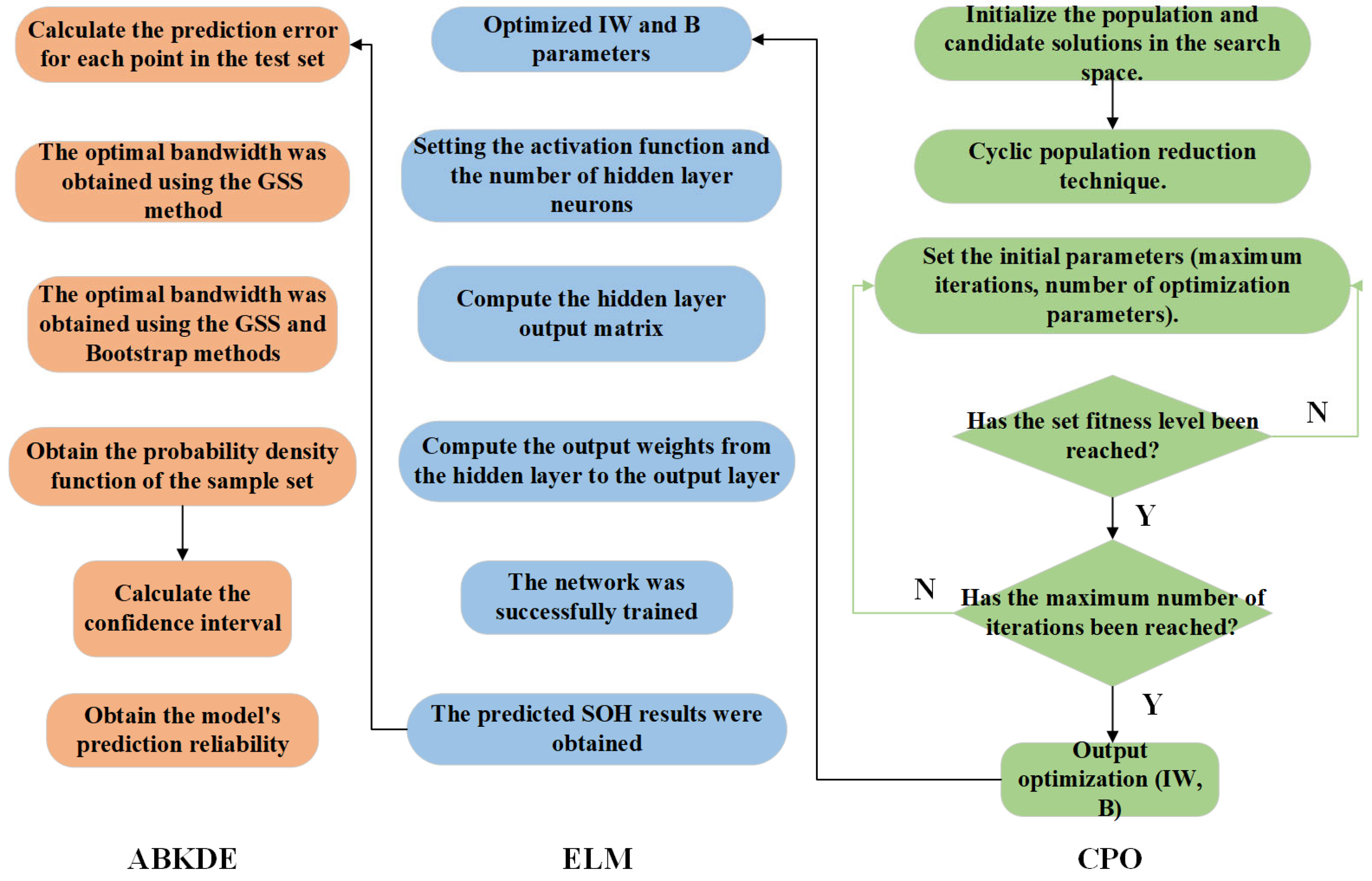
The SOH prediction and uncertainty quantification process based on the CPO-ELM-ABKDE model is shown in Figure 9. In this study, the parameter settings of the CPO algorithm are as follows: the population size is set to 30, and the maximum number of iterations is set to 90. These settings are primarily based on the recommended parameter ranges in the original CPO paper. To further verify their suitability, preliminary comparison experiments were conducted under different parameter combinations. The results indicate that the current configuration achieves a favorable balance between prediction accuracy and computational efficiency.

The overall process can be divided into three main parts, from right to left, CPO optimization, ELM training and prediction, and confidence interval calculation. In the initial stage of CPO optimization, to ensure the coverage of the search space, the algorithm is initialized, the initial population is generated, and candidate solutions are selected within the search space. Then, during the iterative process of the algorithm, CPO adopts a cyclic population reduction technique, gradually eliminating individuals with low fitness to ensure the population converges to a better solution. The maximum number of iterations and the number of optimization parameters need to be set to ensure the algorithm completes the search within a reasonable computational time. In each iteration, the CPO algorithm calculates the fitness of the current population and updates the current optimal solution, gradually approaching the optimal parameter combination. When the population reaches the set fitness level, the optimization process terminates. Otherwise, the iterations continue until the maximum iteration count is reached. Finally, the CPO optimization part outputs the optimized IW and B, providing the optimal parameters for the subsequent ELM training.

Next, the parameters of the hidden layer of the ELM model are set, including the selection of the activation function type and the determination of the number of hidden layer neurons to ensure the network has sufficient learning capability. Then, the input data is passed through the IW and B, and after activation function transformation, the output of the hidden layer is generated. Subsequently, the connection weights from the hidden layer to the output layer are calculated, and the least squares method is used to solve it, allowing the model to quickly fit the data distribution.

In the confidence interval calculation part, the ABKDE method is introduced to analyze the uncertainty of the ELM’s prediction results. First, the prediction error for each data point in the test set is calculated as the basis for the subsequent uncertainty quantification. Then, the GSS and Bootstrap methods are combined to optimize the bandwidth parameter to improve the accuracy of the confidence interval estimation. Based on the optimized bandwidth, the probability density function of the prediction errors is calculated to obtain the probability distribution of the sample set. Using the obtained probability density function, the confidence interval is calculated to quantify the uncertainty range of SOH prediction.

3.7. Evaluation Metrics of the Prediction Model

Since the estimation of lithium-ion battery capacity is essentially a regression problem, the goal is to predict a continuous output value (i.e., battery capacity) through input features (such as voltage, current, etc.). Therefore, it is necessary to choose evaluation metrics suitable for regression tasks. Commonly used metrics in regression model performance evaluation include MAE (mean absolute error) and RMSE (root-mean-square error).

$$MAE={\displaystyle \frac{1}{N}}{\displaystyle \sum _{i=1}^N\left|D_1-D_2\right|},$$

(26)

$$RMSE=\sqrt{{\displaystyle \frac{1}{N}}{\displaystyle \sum _{i=1}^N{\left|D_1-D_2\right|}^2}},$$

(27)

where $D_1$ is the actual battery capacity, $D_2$ is the predicted battery capacity, and $N$ is the number of cycles.

4. Experimental Results and Comparative Analysis

4.1. Verify the Effectiveness and Accuracy of the Algorithm

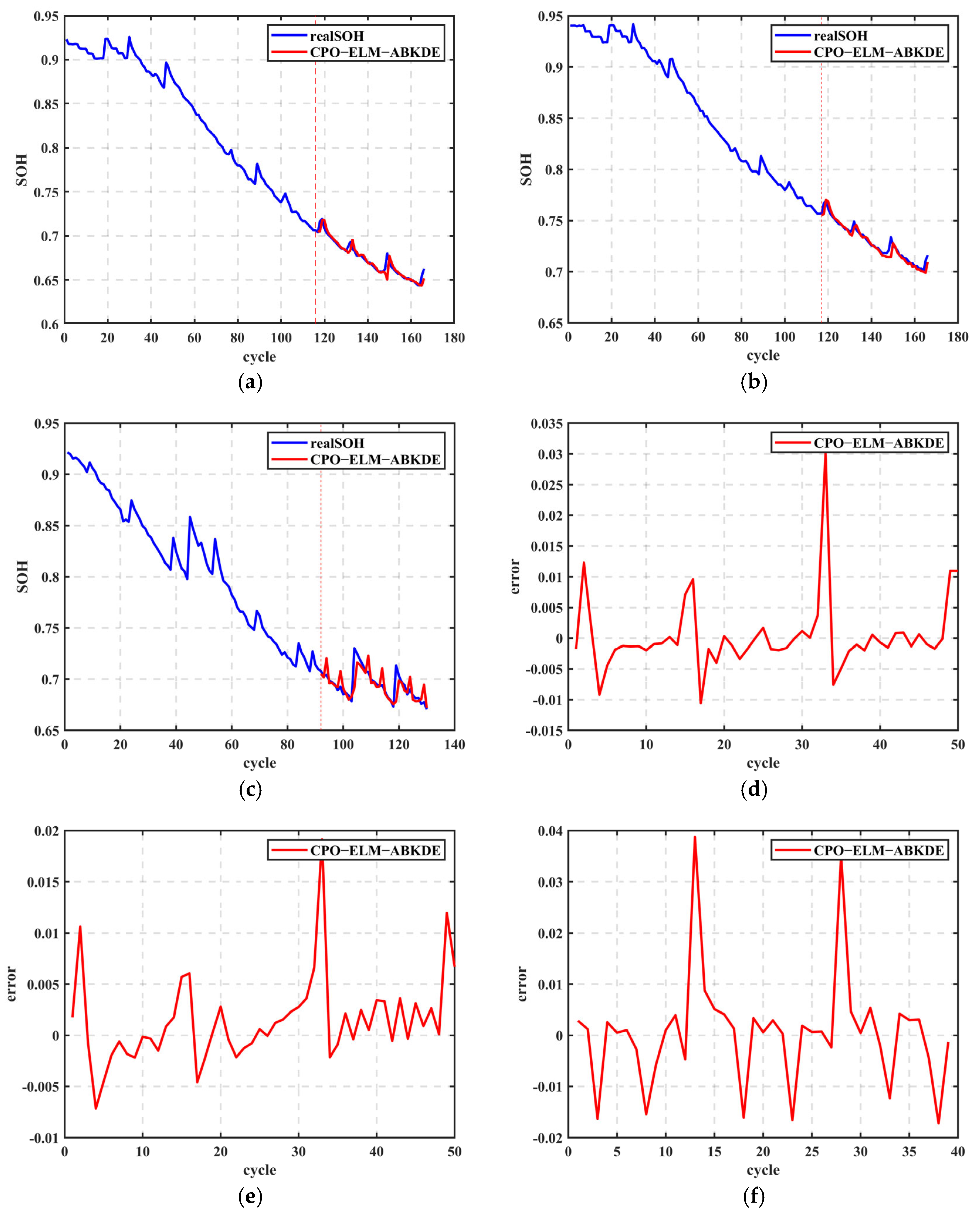
In this study, the SOH of lithium-ion batteries was predicted and analyzed using the CPO-ELM-ABKDE model. First, 70% of the battery data was selected for model training to establish the SOH prediction model. As shown in Figure 10a–c, the model accurately fits the SOH variation trends of batteries B0005, B0007, and B0018. In Figure 10a, the SOH of battery B0005 gradually decreases with cycling, and the CPO-ELM-ABKDE predicted values align closely with the actual values. In Figure 10b, the SOH decline trend of battery B0007 is similarly captured with high accuracy by the model. In Figure 10c, the SOH of battery B0018 exhibits a complex pattern of initial decline, followed by fluctuation, and then further decline. The model still effectively tracks this trend. Moreover, error analysis further validates the model’s accuracy. Figure 10d–f show the prediction error curves for B0005, B0007, and B0018 batteries. In Figure 10d, the error for B0005 fluctuates between −0.015 and 0.035, while in Figure 10e, the error for B0007 lies between −0.01 and 0.02, and in Figure 10f, the error for B0018 is slightly larger but still within the range of −0.02 to 0.04. This indicates that CPO-ELM-ABKDE exhibits good prediction capability and stability. The absence of significant fluctuations in the error further demonstrates the model’s adaptability to different battery degradation modes. 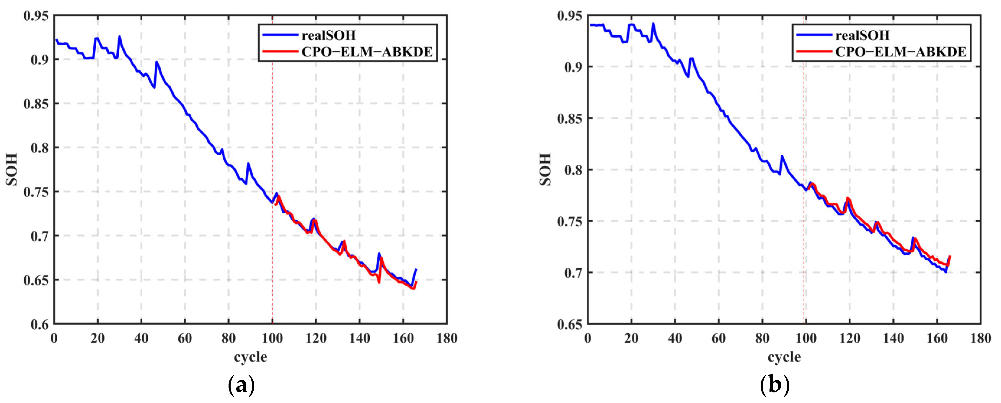Figure 11 shows that when the training set is reduced to 60%, the model’s prediction curve still closely matches the actual value curve. For example, in Figure 11a–c, the SOH predictions for the B0005, B0007, and B0018 batteries remain tightly aligned with the actual values. The corresponding error curves in Figure 11d–f show a slight increase in error, but it remains within a reasonable range. This verifies that the CPO-ELM-ABKDE model maintains high prediction accuracy and stability even with a reduced training set. Even with fewer samples, the model can still effectively capture the SOH change trends, providing accurate battery health state predictions through multi-level optimization and adaptive adjustments.

Table 4. CPO-ELM-ABKDE model prediction results with a 70% dataset.

Battery	MAE	RMSE
B0005	0.0034	0.0061
B0007	0.0029	0.0045
B0018	0.0065	0.0108

shows that when the training set comprises 70% of the data, the CPO-ELM-ABKDE model exhibits excellent stability in SOH prediction for the three battery groups. The MAE ranges from 0.29% to 0.65%, and the RMSE ranges from 0.45% to 1.08%. The absence of significant fluctuations in the error further highlights the model’s adaptability and robustness across different battery samples. This low error level strongly demonstrates the model’s ability to capture SOH variation trends, providing reliable support for accurate battery health assessment.

Table 5. Prediction results of the CPO-ELM-ABKDE model with a 60% dataset.

Battery	MAE	RMSE
B0005	0.0038	0.0063
B0007	0.0044	0.0049
B0018	0.0086	0.0117

shows that when the training set is reduced to 60%, the RMSE and MAE values for batteries B0005, B0007, and B0018 slightly increase, but the prediction accuracy remains high, with MAE ranging from 0.38% to 0.86% and RMSE ranging from 0.49% to 1.17%. The increase in error is controllable. This further validates the excellent performance and stability of the CPO-ELM-ABKDE model in SOH prediction, even with reduced training samples. The model still effectively learns the battery degradation characteristics and maintains high-accuracy predictions.

4.2. Quantifying Prediction Uncertainty

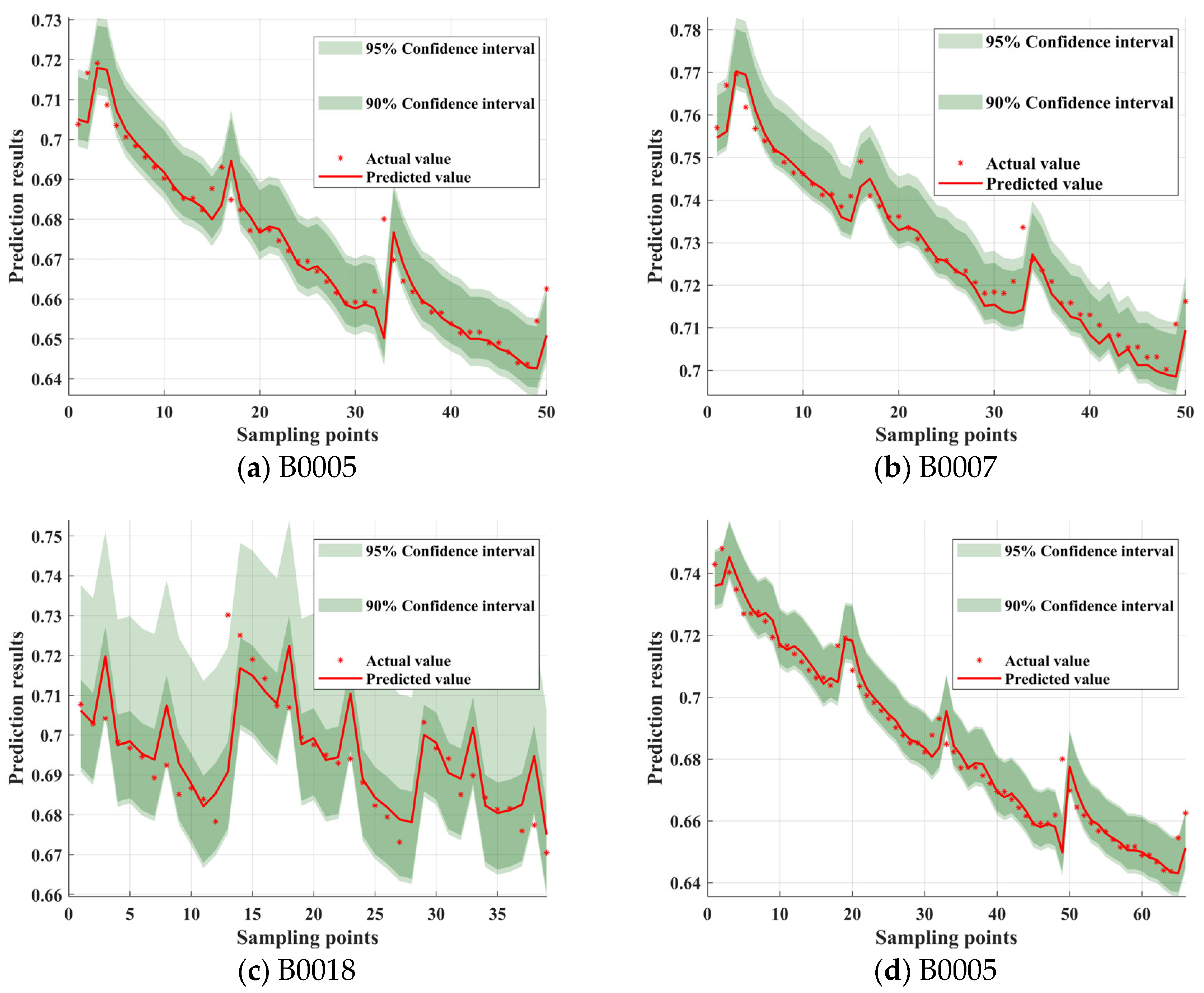
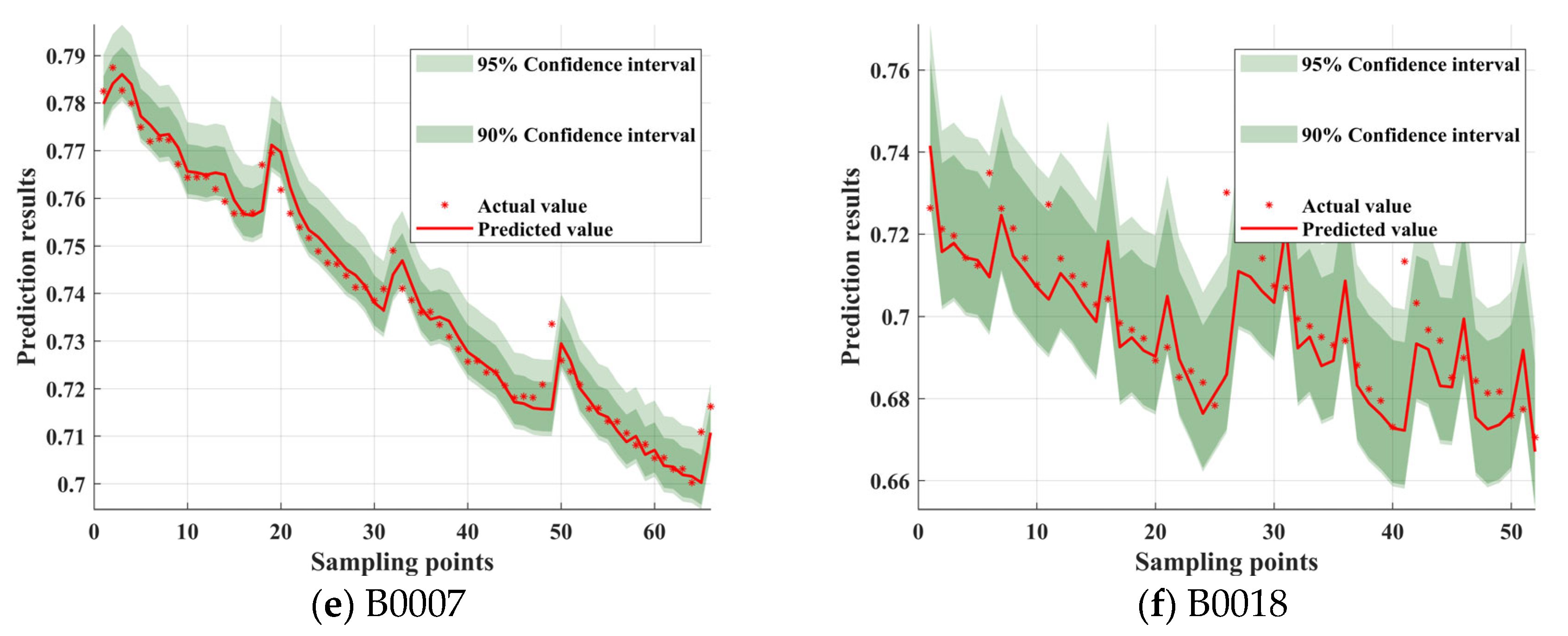
As seen in Figure 12, the model’s predicted values closely match the actual values. From the trends in the different subgraphs, it can be observed that the width of the confidence interval is not fixed but varies with the fluctuations in the data. In regions where SOH changes steadily, such as some descending segments of B0005 and B0007, the confidence interval is narrower, indicating stable predictions with low uncertainty. However, in regions with sharp SOH fluctuations, such as local abrupt points in B0018 and B0005, the confidence interval increases significantly, reflecting the model’s adaptability to high-uncertainty data. During the later stages of rapid SOH decline, the prediction interval width slightly increases, indicating that the model may face higher uncertainty at low SOH levels. This adaptive adjustment characteristic of the interval shows that CPO-ELM-ABKDE, combined with uncertainty quantification, can dynamically adjust the prediction interval based on data features, improving the model’s robustness and reliability.

The confidence interval width is not fixed but varies with data fluctuations. In regions where SOH changes smoothly (e.g., certain descending segments of B0005 and B0007), the confidence interval is narrow, reflecting low uncertainty. In regions where SOH fluctuates significantly (e.g., local spikes in B0018), the confidence interval widens significantly, demonstrating the model’s ability to adapt to high uncertainty. During the rapid SOH decline in the later stages, the prediction interval width slightly increases, indicating higher uncertainty at low SOH levels. This self-adjusting characteristic indicates that the CPO-ELM-ABKDE model incorporates an uncertainty quantification mechanism, dynamically adjusting the prediction interval based on data characteristics, thereby improving the model’s robustness and reliability. The 90% and 95% confidence intervals in Figure 12 show that most actual SOH values fall within the prediction intervals, indicating the model’s excellent coverage at high confidence levels. This is of great significance for battery health management. At the 95% confidence level, the model can be used for battery life early warning, ensuring that the predicted SOH interval covers the actual values, reducing the risk of prematurely or unnecessarily replacing the battery. At the 90% confidence level, the prediction interval is narrower, suitable for daily battery maintenance, providing more accurate SOH estimates and optimizing charge–discharge strategies. In summary, Figure 12 comprehensively demonstrates the prediction accuracy of the CPO-ELM-ABKDE model and the adaptability of the confidence intervals under different SOH variation patterns, providing reliable support for battery health assessment.

In real-world scenarios, this has significant implications for decision making in fields such as finance, engineering, and climate modeling. For instance, in financial forecasting, a wider confidence interval (as observed in B0005) indicates higher uncertainty, suggesting that investment decisions should be approached with caution. Conversely, a narrower interval (as in B0007) reflects higher reliability, enabling more confident planning. Occasional instances where actual values fall outside the predicted intervals (e.g., B0018) highlight the model’s limitations and underscore the need for continuous refinement to improve predictive accuracy in practical applications.

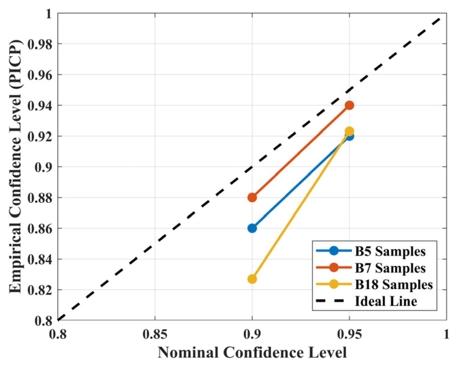
To further validate the statistical effectiveness of the confidence intervals constructed by the ABKDE method, experiments were conducted on three battery datasets—B0005, B0007, and B0018. At different confidence levels, the proportion of the true SOH values falling within the predicted intervals, i.e., the Prediction Interval Coverage Probability (PICP), was calculated. The confidence interval calibration curves were plotted as shown in Figure 13. It can be observed from the figure that all three datasets closely follow the ideal line in terms of overall trend. Under the 95% confidence interval, the empirical coverage rates for B0005, B0007, and B0018 were 92%, 93.5%, and 91.6%, respectively. Under the 90% confidence interval, the empirical coverage rates were 86%, 88%, and 85% for B0005, B0007, and B0018, respectively. These results are highly consistent with the nominal confidence levels. This indicates that the constructed “90%” and “95%” confidence intervals are indeed capable of covering the actual SOH values at rates close to the expected levels in the experiments, demonstrating good statistical interpretability. These results further validate the accuracy and reliability of the CPO-ELM-ABKDE model in uncertainty modeling, showing that ABKDE not only adapts to local fluctuations but also maintains consistency in actual confidence levels, thereby offering strong practical value in battery SOH prediction tasks. Based on the results in

Table 6. p-value calculation.

Battery	Nominal	Empirical	p-Value
B0005	0.95	0.920	0.1786
B0005	0.90	0.860	0.1187
B0007	0.95	0.935	0.3094
B0007	0.90	0.880	0.4142
B0018	0.95	0.916	0.1786
B0018	0.90	0.850	0.0716

, all p-values are greater than the commonly used significance level of 0.05, indicating that the deviations between the actual coverage and the nominal confidence level are not statistically significant. Therefore, the coverage rates are consistent with expectations.

4.3. Comparison of CPO-ELM-ABKDE with Other Models’ Prediction Results

To demonstrate the superiority of the CPO-ELM-ABKDE model in estimating the SOH of lithium batteries, comparisons were made with the ELM, KELM, and DBO-SVR models. The maximum number of iterations, population size, and the number of hidden layer nodes for each model were set to the same conditions. These models were then used to estimate the health status of three lithium batteries, and the estimation curves and errors for these batteries are shown in Figure 14. Panels (a–c) display the SOH prediction results for batteries B0005, B0007, and B0018, respectively, comparing the performance of the ELM, KELM, DBO-SVR, and CPO-ELM-ABKDE models.

By analyzing the SOH curves, the advantages of the CPO-ELM-ABKDE model become clear. In contrast, the ELM, KELM, and DBO-SVR models exhibit larger prediction errors, with overall prediction values being higher than the actual SOH, resulting in less-accurate predictions. The error curves shown in panels (d–f) further confirm the advantages of the CPO-ELM-ABKDE model. As seen, the errors in CPO-ELM-ABKDE remain within a smaller range, with smoother fluctuations and smaller amplitudes compared with ELM and DBO-SVR, demonstrating its good stability. Particularly during the later stages of battery degradation, the error in CPO-ELM-ABKDE is significantly smaller than those in the other models, indicating its strong generalization capability across different life stages. Overall, the CPO-ELM-ABKDE model, by integrating adaptive kernel density estimation and swarm intelligence algorithms, greatly enhances prediction accuracy, stability, and robustness, providing a more reliable and efficient solution for battery SOH prediction.

From the data in

Table 7. SOH prediction errors of different battery models.

	B0005		B0007		B0018
Model	RMSE	MAE	RMSE	MAE	RMSE	MAE	Average Runtime
ELM	0.0258	0.0232	0.0236	0.0212	0.0239	0.0176	0.15 s
KELM	0.0135	0.0124	0.0154	0.0136	0.0126	0.0110	0.5 s
DBO-SVR	0.0077	0.0068	0.0093	0.0072	0.0122	0.0099	1.5 s
CPO-ELM-ABKDE	0.0061	0.0034	0.0045	0.0029	0.0108	0.0065	3 s

, it is clear that the RMSE and MAE values differ among the models for different battery datasets. The CPO-ELM-ABKDE model shows the lowest errors, indicating the best SOH prediction performance. The ELM model consistently exhibits the highest RMSE and MAE across all datasets, indicating larger prediction errors and weaker stability. KELM, compared with ELM, shows significant improvement, especially for the B0005 and B0007 datasets, where both RMSE and MAE are substantially reduced, but it still does not reach optimal performance. The DBO-SVR model further reduces errors compared with KELM, suggesting an improvement in SOH prediction accuracy. However, its prediction errors are still higher than those of CPO-ELM-ABKDE. For example, in the B0005 dataset, the CPO-ELM-ABKDE model’s RMSE is only 0.0061, and the MAE is 0.0034, reducing RMSE and MAE by 20.78% and 50%, respectively, compared with DBO-SVR’s 0.0077 and 0.0068. This decreasing trend is similarly significant for the B0007 and B0018 datasets, further demonstrating that the CPO-ELM-ABKDE model is superior in prediction accuracy and more reliable in stability.

The CPO-ELM-ABKDE model demonstrated the lowest RMSE and MAE across all datasets (B0005, B0007, and B0018). All experiments were conducted on a laptop equipped with a 13th Gen Intel^® Core™ i7-13700H processor and 16 GB of RAM. The datasets B0005 and B0007 each contain 166 samples, while B0018 contains 130 samples, and 70% of each dataset was used for training. Although this model exhibited relatively longer computation times (averaging 3 s), its high prediction accuracy suggests a better balance between precision and computational load. Among the models compared, ELM had the shortest computation time (average of 0.15 s); however, its prediction errors were significantly higher. KELM achieved faster computation than CPO-ELM-ABKDE (approximately 0.5 s on average), yet it still lagged behind in terms of error reduction. DBO-SVR required a longer computation time (average of 1.5 s), slower than both ELM and KELM, but yielded better predictive performance than either of them. Despite its relatively longer runtime, the CPO-ELM-ABKDE model’s enhanced accuracy may render it more appealing for real-time applications, particularly in scenarios requiring high precision, such as battery health monitoring and lifecycle prediction.

In order to validate the robustness and reliability of the performance improvements achieved by the CPO-ELM-ABKDE model over baseline models, statistical significance testing was conducted. Using the B0005 dataset as a case study, the MAE and RMSE values obtained from 10 independent runs of the CPO-ELM-ABKDE model were compared with those of ELM, KELM, and DBO-SVR using paired t-tests. This approach ensures fairness and consistency by evaluating differences in prediction accuracy under identical experimental conditions. As shown in

Table 8. The t-test for the model.

Model	p-Value (MAE)	p-Value (RMSE)
ELM	1.5390 × 10−16	2.4963 × 10−20
KELM	2.4963 × 10−20	1.6864 × 10−16
DBO-SVR	2.5455 × 10−9	1.6378 × 10−10

, all p-values related to the comparisons of MAE and RMSE are significantly lower than the conventional threshold of 0.05, indicating that the observed improvements from CPO-ELM-ABKDE are not due to random fluctuations. These statistically significant results confirm the superior predictive capability of the proposed model and demonstrate that its performance enhancements are consistent and reproducible.

4.4. Verifying the Generalizability of the CPO-ELM-ABKDE Model

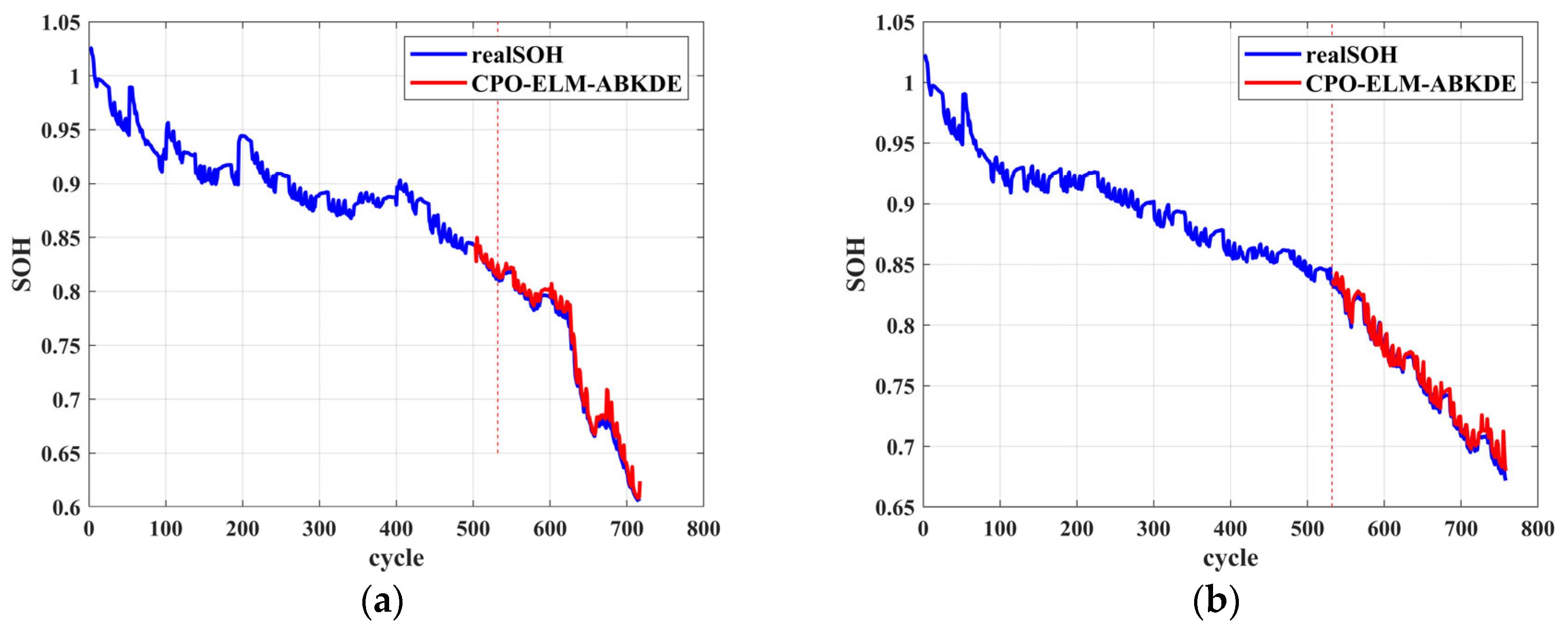
The effectiveness of the CPO-ELM-ABKDE model in battery degradation prediction was verified through the analysis of NASA-provided datasets for batteries B0005, B0007, and B0018. To further verify the generalizability of the CPO-ELM-ABKDE model, the CS2-35 and CS2-37 battery datasets from the University of Maryland were used for prediction. The Maryland battery datasets are widely utilized in battery degradation studies. These datasets record the capacity-fading process of batteries under specific charge–discharge conditions and include SOH data over multiple cycles. Using the same health features as selected for the NASA datasets and without modifying the structural parameters of the model, the SOH predictions were obtained using the CPO-ELM-ABKDE model and then compared with the actual SOH values.

As shown in Figure 15, the prediction curves of the CPO-ELM-ABKDE model closely follow the actual SOH degradation trend. For the CS2-37 battery, although the degradation pattern is similar to that of CS2-35, the degradation rate is slightly different. The SOH of CS2-37 begins to decline rapidly around the 400th cycle, and the CPO-ELM-ABKDE model is still able to accurately predict this change, demonstrating its adaptability to different degradation behaviors.

To quantitatively evaluate the model’s prediction performance, RMSE and MAE were used as metrics.

Table 9. Prediction errors of the CPO-ELM-ABKDE model on the Maryland battery dataset.

Battery	MAE	RMSE
CS2-35	0.0051	0.0067
CS2-37	0.0048	0.0062

presents the prediction error results for the CS2-35 and CS2-37 batteries. The MAE values for both batteries are less than 0.51%, and the RMSE values are less than 0.67%. These error levels indicate that the CPO-ELM-ABKDE model achieves high prediction accuracy on both datasets, fully validating the accuracy and robustness of the proposed model. According to references [40,41],

Table 10. Comparison of RMSEs between CPO-ELM-ABKDE and Transformer on the NASA dataset.

	CPO-ELM-ABKDE	Transform
Battery	RMSE	RMSE
B0005	0.0061	0.0098
B0007	0.0045	0.0173
B0018	0.0108	0.0320

and

Table 11. Comparison of RMSEs between CPO-ELM-ABKDE and Transformer on the CALCE dataset.

	CPO-ELM-ABKDE	Transform
Battery	RMSE	RMSE
CS2-35	0.0067	0.0104
CS2-37	0.0062	0.0075

were derived, which show that the RMSE of the CPO-ELM-ABKDE model is significantly better than that of the Transformer model across five different battery datasets (B0005, B0007, B0018, CS2-35, and CS2-37). For example, on the B0007 battery, the RMSE of CPO-ELM-ABKDE is 0.0045, while the Transformer’s RMSE is 0.0173; on CS2-35, the RMSE of CPO-ELM-ABKDE is 0.0067, while the Transformer’s RMSE is 0.0104. These results demonstrate that the proposed method offers higher prediction accuracy and stronger generalization ability in the SOH prediction task.

To further evaluate the robustness of the model, the B0005 dataset was used as the training set and the B0007 dataset as the testing set, resulting in an MAE of 0.0075 and an RMSE of 0.0092. In the reverse setup, where B0007 served as the training set and B0005 as the testing set, the model achieved an MAE of 0.0133 and an RMSE of 0.0138. These results confirm that the model exhibits strong generalization capability across different batteries, even when trained and tested on independent datasets.

5. Conclusions

In response to the issue of SOH prediction accuracy for lithium-ion batteries, this study proposed an SOH estimation method based on the CPO-ELM-ABKDE model. The following conclusions were drawn based on the NASA dataset:

• HF is extracted from the charging voltage curve and IC curve, and the correlation between HF and capacity/SOH is analyzed using Pearson and Spearman correlation theories, with HF that has a small correlation with capacity being excluded.
• The traditional ELM randomly generates IW and B, leading to unstable prediction performance. The CPO algorithm is introduced to optimize IW and B, improving ELM’s prediction ability and stability.
• Since ELM can give only a fixed prediction value and cannot provide prediction uncertainty, ABKDE is introduced to quantify prediction uncertainty, allowing the prediction interval to adaptively adjust according to data characteristics and enhancing model stability.
• Through experiments with different battery aging datasets, the CPO-ELM-ABKDE model’s prediction performance significantly outperforms other methods, with RMSE and MAE both below 0.86% and 1.17%, respectively.

The experimental results indicate that the CPO-ELM-ABKDE model demonstrates robust stability and predictive capability across multiple battery aging datasets, suggesting its potential adaptability to various SOH degradation patterns. The use of CPO contributes to improved model performance by adaptively optimizing network parameters according to battery characteristics, while the integration of ABKDE enhances the robustness of SOH predictions by estimating confidence intervals. However, the model’s generalization ability still requires further validation when applied to more complex or atypical degradation scenarios. With the rapid development of electric vehicles, battery health management has become increasingly critical. The CPO-ELM-ABKDE model shows promise for real-time SOH monitoring, enabling early prediction of battery degradation, thus extending battery lifespan and improving driving range and safety. In grid energy storage systems, this model can be employed to monitor battery health, support adaptive usage strategies, and facilitate timely replacement of degraded batteries, thereby enhancing system reliability and operational efficiency. By supporting the extension of battery life and enabling proactive maintenance strategies, the proposed method contributes to reducing electronic waste and conserving critical raw materials, which aligns with key goals of environmental sustainability and circular economy principles. It also promotes the efficient utilization of renewable energy systems by improving energy storage reliability, thereby supporting long-term sustainable energy transitions.

From an implementation perspective, although CPO and ELM theoretically offer strong optimization and prediction capabilities, computational efficiency and response time are critical factors for real-time applications in large-scale battery management systems. As the volume of battery data increases, the computational complexity of the CPO algorithm may become a bottleneck. Therefore, in practical deployment, it may be necessary to incorporate hardware acceleration or adopt more efficient optimization strategies—such as parallel or distributed computing—to enhance real-time prediction performance. While ABKDE provides valuable uncertainty quantification for the prediction results, it may fail to fully capture all uncertainties under extreme conditions such as highly imbalanced datasets or abrupt fluctuations in battery behavior, thereby affecting the reliability of the predictions. Consequently, the model requires regular updates and adjustments during real-world applications to accommodate potential environmental changes and newly emerging degradation patterns.

Although the CPO-ELM-ABKDE model performs well in SOH prediction, it has some limitations. It relies on high-quality charging data, which may be affected by sampling errors in practice. The CPO and ABKDE steps increase training time, limiting real-time deployment. External factors like temperature are not considered, and the model depends on large amounts of labeled SOH data, which are hard to obtain. Due to the limited availability of high-quality, multi-temperature cycling data in public datasets at this stage, this work is restricted to ambient temperature data. Future work may focus on introducing multimodal features, optimizing the model, and applying transfer learning to improve adaptability and online application.

Future research can further explore the following areas: discovering more efficient parameter optimization strategies to reduce computational costs and improve the real-time prediction capability of the model and studying more advanced uncertainty quantification methods to further enhance prediction reliability and adaptability.