Geospatial Analysis of Urban Warming: A Remote Sensing and GIS-Based Investigation of Winter Land Surface Temperature and Biophysical Composition in Rajshahi City, Bangladesh

Abstract

This study investigates urban warming in Rajshahi City, Bangladesh, by examining changes in land surface temperature (LST) from 1990 to 2023 and exploring its relationship with key biophysical factors. LST was derived from Landsat thermal imagery, and both spatial and temporal variations were analyzed using Geographic Information Systems (GIS). Key biophysical indices, including Normalized Difference Vegetation Index (NDVI), Normalized Difference Built-up Index (NDBI), Normalized Difference Water Index (NDWI), Normalized Difference Moisture Index (NDMI), and Normalized Difference Bareness Soil Index (NDBSI), were calculated using corresponding Landsat satellite sensors, and they evaluated the impact of LULC types (vegetation, water, soil, and built-up areas) on thermal variations. LULC was derived following the Support Vector Machine classification technique. The Urban Thermal Field Variance Index (UTFVI) was employed to assess surface urban heat island (SUHI) effects, warming conditions, ecological stress, and thermal comfort zones. Spatial trend and hotspot analyses of LST change were performed using spatial trend analysis and the Getis-Ord Gi* statistic, respectively. Linear regression analysis examined the relationship between LST and biophysical indices. Results show that winter mean LST increased by 2.66 °C during the 33-year period, with maximum LST rising by 4.29 °C. The most significant warming occurred in central-northern, central-western, and south-eastern zones. The rise in LST and the growing intensity of SUHI effects are largely due to urban growth, especially where green spaces and water bodies have been replaced by impervious surfaces. Hotspot analysis identified clusters of high-temperature zones, while UTFVI analysis confirmed a marked expansion of strong heat island conditions, especially in central urban areas. Linear regression results showed notable links between LST and key biophysical variables, where higher LST values were commonly linked to greater built-up density and declines in vegetation cover and surface water. Overall, the results highlight the need for better urban planning approaches such as increasing green cover, using permeable materials, and adopting strategies that can adapt to climate impacts. This study presents a framework for analyzing urban climate dynamics that can be adapted to other rapidly growing cities, aiding efforts to promote sustainable development and build urban resilience.

1. Introduction

Air and surface temperature patterns in urban areas often differ from those of rural settings, largely due to changing patterns in land use and land cover (LULC). Such variations play a crucial role in influencing the urban climate. As cities expand, the natural landscape is replaced with roads, buildings, and other impervious surfaces, altering the local climate and energy balance [1,2,3]. The dominance of these anthropogenic surfaces alters energy balance and local climate, significantly impacting both land surface temperature and air temperature. The urban climate is shaped by the built environment of the city and differs notably from surrounding rural areas due to surface modifications and human activities. Urbanization, coupled with large-scale alterations in surface and atmospheric properties, contributes to a measurable rise in urban temperatures. Recent studies suggest that many cities are experiencing warming at rates up to twice or more the global average (0.20 °C per decade), often due to reduced vegetation and increased energy use [4,5,6]. For example, Phoenix (USA) has seen a temperature rise of about 0.86 °C per decade, while Shanghai (China) warms at roughly 0.37 °C per decade due to rapid urbanization. In western Sydney, the rate is around 0.65 °C per decade. On a broader scale, megacities across Asia have experienced average warming rates of 0.69 °C per decade [4,5,6,7,8]. These trends highlight the intensifying impact of urban heat driven by reduced vegetation and increased energy use. During winter, the urban heat island effect often intensifies as vegetation cover decreases and human-generated heat becomes a larger contributor to local warming. Cities such as Beijing, New York, and London have documented temperature differences of 3–5 °C compared to nearby rural areas [4,5,6,7]. In the United States, urban air temperatures have been found to exceed those of nearby natural land cover by up to 5.6 °C, with New York showing differences above 5 °C [8]. These differences in surface temperature, known as the surface urban heat island (SUHI) effect, can influence energy demand, air pollution, and thermal stress in city environments [9,10,11,12,13,14,15]. LST, measured by satellites or ground sensors, is a key metric used to analyze heat patterns across urban areas. The measure indicates the temperature of the land’s exterior layer, covering vegetation, soil, urban structures, and various surface elements [16,17]. Remote sensing technologies enable LST estimation by capturing infrared radiation emitted by surface materials [18,19], making it an indispensable tool for analyzing urban thermal dynamics and supporting climate-resilient planning.

Monitoring LST is essential not only for understanding urban heat but also for modeling broader climate-related processes, especially as they relate to land changes, particularly concerning warming trends and the greenhouse effect. Understanding and tracking urban climate change are essential for comprehending the broader urban environment, given the intricate spatial and temporal variations inherent within urban areas [20]. Recent research has placed a significant emphasis on observing and monitoring LST and SUHI effects across diverse landscapes, owing to their profound impacts on local weather and climate patterns, particularly within urban settings [21,22,23,24,25]. However, accessing comprehensive historical climate data, including temperature, precipitation, and humidity, remains challenging, especially in developing countries like Bangladesh, where large-scale and time series observational datasets are scarce. Given the limitations in observed data availability, LST emerges as a potent proxy for monitoring urban climate change, as historical spatial data of LST can be readily obtained from thermal sensors aboard satellites such as Landsat, the Moderate Resolution Imaging Spectroradiometer (MODIS), the National Oceanic and Atmospheric Administration (NOAA), and the Television Infrared Observation Satellite (TIROS) [26,27]. Sensors like the Landsat Thematic Mapper (TM), the Enhanced Thematic Mapper Plus (ETM+), and the Operational Land Imager (OLI) are widely utilized for exploring LST dynamics and assessing their associations with other urban components [28]. The significance of LST transcends mere climate monitoring; it also plays a pivotal role in regulating the energy and water balance within a given area, thus exerting influence over its local climate. Advances in remote sensing technologies and analytical methodologies enable the effective calculation of LST, facilitating its monitoring over extended periods [29]. Consequently, continuous monitoring of LST through remote sensing offers crucial insights into urban climate change conditions and the surface physical properties that drive various environmental processes [30,31].

Urban expansion induces variations in LST, resulting in elevated temperatures in specific locations known as the SUHI effect. LST dynamics have been extensively scrutinized across numerous cities worldwide, with a wealth of studies documenting these phenomena over recent decades [21,32,33,34,35,36,37,38,39,40,41]. Pioneering investigations into SUHI, utilizing satellite-derived LST data, were conducted by the authors of [42] to examine temperature patterns along the mid-Atlantic coast. Subsequently, Refs. [43,44] utilized NOAA data to identify urban heat island (UHI) effects. Since then, a plethora of studies have delved into SUHI and LST patterns, leveraging data collected from a variety of remote sensing sources, such as satellite systems, aerial platforms, and ground-based monitoring devices [38,45,46,47]. In contemporary research, Landsat sensor data have emerged as a cornerstone for analyzing SUHI patterns, urban LST dynamics, and elucidating the interplay between LST and LULC [41,46]. Similarly, studies focusing on spatio-temporal analyses of LST using remote sensing thermal data in Bangladeshi cities have surfaced, predominantly utilizing Landsat satellite data to examine LULC changes and LST patterns, given the significant transformations in urban landscapes [25,40,47,48,49,50,51,52,53,54]. Despite these efforts, studies investigating LST and SUHI as pivotal climate parameters for monitoring urban climate change and discerning the influence of biophysical parameters on such changes, particularly in Bangladeshi cities, remain sparse [25,47,48]. The escalating impact of urban heat has spurred heightened interest among researchers and urban planners, fueled by extensive infrastructural and economic growth in urban areas. However, the scientific understanding and comprehensive analysis of urban thermal phenomena and related climate changes remain limited [55]. In particular, studies focusing on LST variations and warming dynamics during the winter season are scarce. Yet, investigating winter warming is critical for gaining a holistic understanding of urban ecological processes and environmental conditions. The rise in urban winter temperatures has become an increasingly pressing issue in the context of climate change, largely driven by the UHI effect. In densely built environments, impervious surfaces absorb and retain heat, causing winter temperatures in cities to be noticeably higher than in nearby rural areas. This warming trend not only alters local climatic conditions but also disrupts ecological stability within urban ecosystems. One notable consequence is the shortening of the winter season, a pattern now evident in many tropical cities. Warmer winters also create favorable conditions for the year-round survival of pests and the spread of disease vectors, while posing challenges to urban vegetation and wildlife. In the broader framework of climate change, this phenomenon underscores the critical need for climate-responsive urban planning, the integration of green infrastructure, and the promotion of adaptive strategies to reduce heat stress and enhance the resilience and livability of cities.

Therefore, this study underscores the importance of LST and SUHI as critical phenomena for monitoring urban climate change, particularly within the context of urban warming scenarios in winter and in response to biophysical compositions, focusing on the Rajshahi metropolis. Particularly, the aim is to analyze LST alongside biophysical components for urban warming change and SUHI dynamics, primarily utilizing satellite remotely sensed data. Also, this study seeks to enhance the comprehension of urban warming processes and research findings-based planning for long-term urban sustainability by highlighting these critical phenomena. This investigation focuses on achieving the following specific aims: (i) examine the nature of urban warming through changes in LST from 1990 to 2023; (ii) identify the spatio-temporal patterns of LST within the city area; (iii) analyze the spatial relationship between LST and selected biophysical indices over time; and (iv) detect spatial trends and hotspots of LST changes. These objectives were achieved by quantifying LST, analyzing warming scenarios, investigating LULC changes, assessing multiple biophysical indices, and detecting spatial trends and hotspots. The uniqueness of the present study lies in its inclusive exploration of the spatio-temporal patterns of urban warming and changing patterns in Rajshahi City, focusing on recent LST dynamics and related phenomena, which have not been previously studied in the area. By analyzing urban warming through changes in LST and finding its relationship with important biophysical urban components, this study indicates the significance of proper planning to maintain adequate green spaces and surface water features and to adopt climate-adaptive urban strategies. The approach and analytical framework of this study are transferable to other urban areas in developing countries to support effective urban planning aimed at mitigating the adverse impacts of warming and promoting sustainable urban development.

2. Data Used and Methods

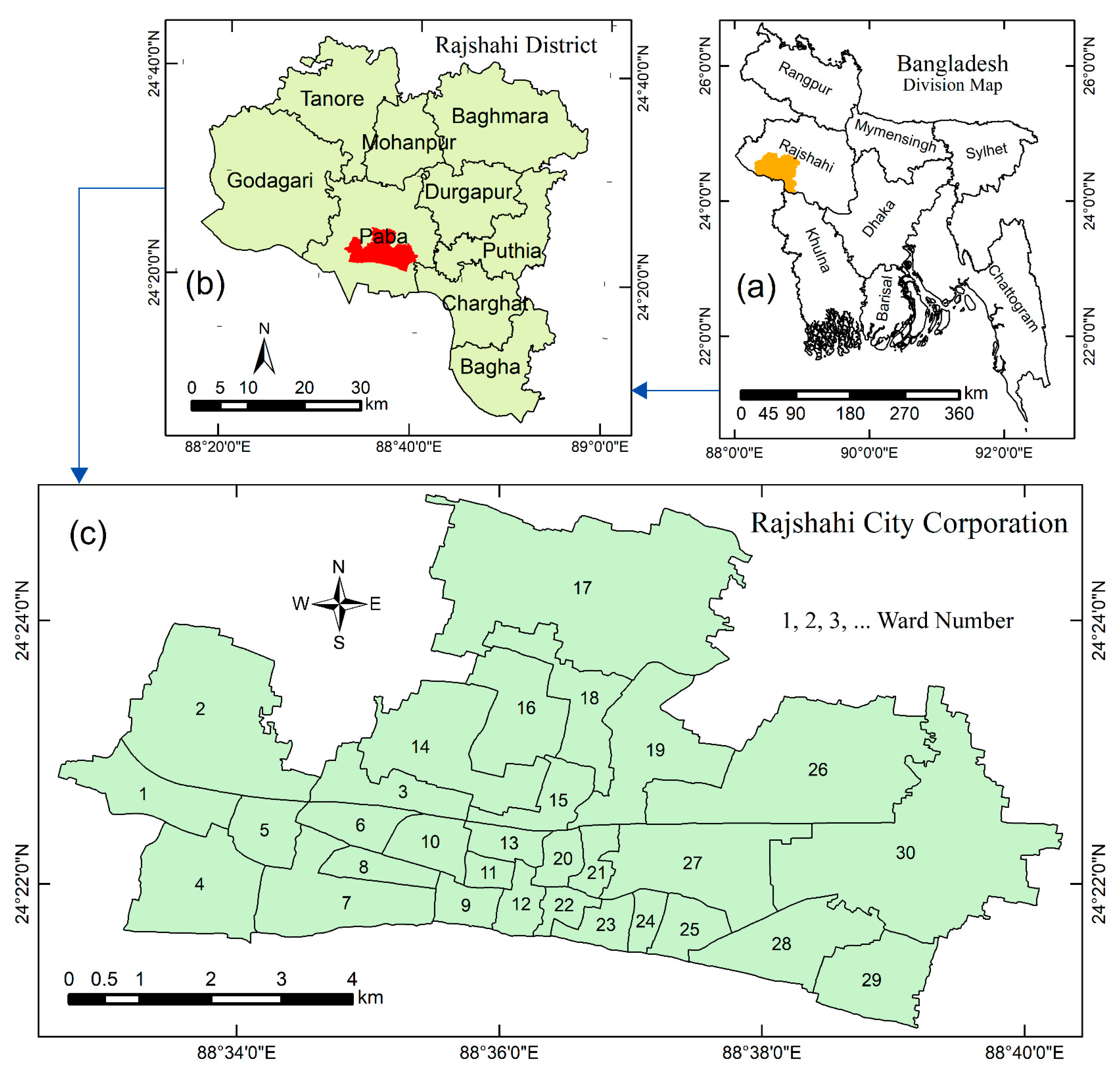
2.1. Study Area

Rajshahi City Corporation (RCC), situated in the north-west region of Bangladesh, is designated as the focal area of the present research endeavor. Encompassing an area of 48 km², the city is strategically positioned between the latitude and longitude 24°12′ to 24°42′ N and 88°15′ to 88°50′ E, respectively [56] [Figure 1]. Because of vast urban growth and urbanization during the last few decades and to know the LST pattern, this city was purposely selected. Serving as a divisional headquarters, RCC comprises 30 administrative wards. The city is nestled along the banks of the Padma River amidst verdant landscapes and fertile plains. The climate of the city is tropical monsoon, featuring an average annual temperature of 24.5 °C and rainfall measuring 1448 mm per year. In winter, temperature ranges from 9 °C to 30 °C with almost no rainfall in this season. Furthermore, the region experiences significant variability in annual rainfall patterns, a factor that can potentially exacerbate temperature fluctuations in the area [57,58,59]. It is important to note that the study area is not prone to flooding, and the analysis was conducted for the month of November, which typically experiences very little to no rainfall. Therefore, the influence of precipitation or flood-related effects on LST during the study period is considered negligible. As a divisional headquarters, Rajshahi has undergone accelerated urban growth in recent decades, becoming home to approximately one million inhabitants. The population has exhibited an annual growth rate of 2.88% from 1990 to 2022, as reported by Bangladesh Bureau of Statistics [56]. This urban development has noticeably altered the city’s landscape, with open and agricultural lands being converted into built-up areas, thereby impacting the urban climate. The unchecked growth and unrestricted development of built-up areas, along with the reduction in urban green spaces, water bodies, fallow lands, and croplands, have adversely affected the city’s environmental quality and overall resilience, particularly leading to warming trends in urban areas [59]. Consequently, detailed information on urban climate dynamics, particularly surface temperature variations and associated biophysical compositions, is indispensable for informed city development and sustainable expansion efforts. The present study is meticulously designed to analyze the dynamics of land surface temperature, the level of urban warming, and its geospatial patterns over the period spanning 1990 to 2023 in the Rajshahi City Corporation of Bangladesh, aiming to shed light on the evolving urban climate dynamics and contribute to informed decision-making processes for the city’s sustainable future.

2.2. Data Used

To extract and analyze the LST of the study area, Landsat TM, ETM+ and OLI sensors’ multispectral images were acquired for the years 1990, 2000, 2010, and 2023. The details of the remote sensing datasets are presented in

Table 1. Details of satellite datasets.

Sensor	Sensor	Data Level	Date	Band Used	Radiometric Resolution	Spatial Resolution
Landsat 5	TM	Level 1	14 November 1990 and 5 November 2010	Blue (b1) Green (b2) Red (b3) NIR (b4) SWIR-1 (b5) Thermal (b6) SWIR-2 (b7)	0.45–0.52 µm 0.52–0.60 µm 0.63–0.69 µm 0.76–0.90 µm 1.55–1.75 µm 10.40–12.50 µm 2.08–2.35 µm	30 30 30 30 30 120 (30) * 30
Landsat 7	ETM+	Level 1	17 November 2000	Blue (b1) Green (b2) Red (b3) NIR (b4) SWIR-1 (b5) Thermal (b6) SWIR-2 (b7)	0.45–0.52 µm 0.52–0.60 µm 0.63–0.69 µm 0.76–0.90 µm 1.55–1.75 µm 10.40–12.50 µm 2.08–2.35 µm	30 30 30 30 30 120 (30) * 30
Landsat 8	OLI	Level 1	3 November 2023	blue (b2) Green (b3) Red (b4) NIR (b5) SWIR-1 (b6) SWIR-2 (b7) TIRS-1 (b10)	0.45–0.51 µm 0.53–0.59 µm 0.64–0.67 µm 0.85–0.88 µm 1.57–1.65 µm 2.11–2.29 µm 10.6–11.19 µm	30 30 30 30 30 30 100 (30) *

* Resampled to 30 m.

. All data were sourced from the United States Geological Survey (USGS) and downloaded using the GloVis portal (http://glovis.usgs.gov (accessed on 10 September 2024)). Additionally, other spatial data, including city boundaries, ward boundaries, and field data, were obtained from the Rajshahi City Corporation office, the Center for Environment and Geographic Information Services (CEGIS), and the Local Government Engineering Department (LGED), collected using Global Positioning System (GPS) and observation techniques for the study. For spatial analysis, datasets were resampled to a 30 m resolution using ArcGIS 10.6.1.

2.3. Methods

2.3.1. Pre-Processing of Landsat Data

Geometrically corrected Level-1 Landsat imagery was utilized and further processed to enhance the accuracy of the analysis. As the initial step in pre-processing, atmospheric correction was applied to all visible bands using the Dark Object Subtraction (DOS) technique. This image-based method, developed by [60], is extensively applied in remote sensing to mitigate the effects of atmospheric scattering, particularly haze, by estimating and subtracting the path radiance component. However, Albedo, which influences land surface temperature by affecting the amount of solar radiation absorbed or reflected by the surface, is implicitly accounted for through the surface reflectance data obtained using the DOS technique. The DOS method assumes that certain surface features, such as deep-water bodies or shadowed areas, have near-zero reflectance in the visible spectrum. By identifying the darkest pixels in each band, the atmospheric path radiance is estimated and subtracted from all pixels in that band. DOS is favored for its simplicity, ease of application, and independence from in situ atmospheric measurements. It is a widely accepted approach within the geospatial community for correcting light scattering effects [61]. In this study, the DOS module of the ENVI 5.1 image processing software was employed for atmospheric correction. For LST calculations, we followed the methodology outlined in the Landsat User Guide, which recommends using Digital Number (DN) values and converting them to radiance for the radiometric correction of the thermal bands [62]. The detailed procedure is discussed in the following section. The DOS method is not well-suited for thermal bands, and alternative atmospheric correction techniques—such as the Radiative Transfer Equation—require numerous input parameters, making accurate correction of thermal data more complex. Given that the study area features relatively flat terrain and the Landsat imagery was acquired during the dry winter season, typically associated with lower atmospheric water vapor, atmospheric interference in the thermal infrared bands is hence expected to be minimal [63,64]. Therefore, we adopted the methodology recommended by [62], which has been commonly used in earlier studies to estimate LST in diverse geographic settings [25,29,30,31,36,37,38,51,54,65]. In this study, atmospherically corrected imagery was used to derive surface emissivity and other biophysical indices. Incorporating surface emissivity into LST calculations is essential, as it corrects for the radiative transfer between the Earth’s surface and the satellite sensor, thereby enhancing the accuracy of temperature estimates. Further details on the LST computation from thermal data are provided in the following section.

2.3.2. Retrieval of LST from Thermal Landsat TM and ETM+ Images (for 1990, 2000, and 2010)

To compute LST using Landsat TM, ETM+, and OLI data for the years 1990, 2000, 2010, and 2023, the following five steps were employed:

• Step 1: Convert DN (Digital Number) Value to Radiance ($L_{\mathsf{\lambda }}$)

In this step, the digital number (DN) values from the Landsat data were converted into spectral radiance. For Landsat TM and ETM+, spectral radiance was calculated using Equation (1) [62], while for Landsat OLI, Equation (2) [66] was used.

$$L_{\mathsf{\lambda }}={\displaystyle \frac{\left(L_{max \mathsf{\lambda }}-L_{min \mathsf{\lambda }}\right)}{\left(Q_{cal max}-Q_{cal min}\right)}}\times \left(Q_{cal}-Q_{cal min}\right)+L_{min\mathsf{\lambda }}$$

(1)

where $L_{\lambda }$ = spectral radiance (watts/(m² × sr × μm) [watts per square meter per steradian per micrometer], $L_{max \lambda }$ = radiance maximum for the thermal band, $L_{min \lambda }$= radiance minimum for thermal band, $Q_{cal}$= DN value of the thermal band (Band 6 for Landsat TM 5 and ETM⁺), $Q_{cal max}$= the maximum quantized calibrated pixel value of the thermal band, and $Q_{cal min}$= the minimum quantized calibrated pixel value of the thermal band. $L_{min \lambda }$, $Q_{cal max}$, and $Q_{cal min}$ values can be found in the metadata file.

$$L_{\mathsf{\lambda }}={MSF}_{\mathsf{\lambda }}\times Q_{cal}+{ASF}_{\mathsf{\lambda }}-O_i$$

(2)

where $L_{\lambda }$ = spectral radiance (watts/(m² × sr × μm) [Watts per square meter per steradian per micrometer], ${MSF}_{\lambda }$ = radiance multiplicative scaling factor for the band (RADIENCE_MULTI_BAND_10), ${ASF}_{\lambda }$= radiance additive scaling factor for the band (RADIENCE_ADD_BAND_10), $Q_{cal}$= DN value of the thermal band (here Band 10), and $O_i$= correction value (0.29) for Band 10 of Landsat OLI [67,68]. ${MSF}_{\lambda }$ and ${ASF}_{\lambda }$ values can be found in the metadata file.

• Step 2: Convert Radiance to At-sensor Brightness Temperature (°C) (${\mathsf{\tau }}_{\mathit{c}}$)

Here, to change radiance to At-sensor Brightness Temperature in degrees Celsius, Equation (3) was applied [65,68,69,70].

$${\mathsf{\tau }}_c={\displaystyle \frac{k_2}{Ln\left(\frac{k_1}{L_{\mathsf{\lambda }}}+1\right)}}-273.15$$

(3)

where ${\tau }_c$ = At-sensor Brightness Temperature, in °C, $k_1$= pre-launch calibration thermal constants for the band (K1_CONSTANT_BAND_6 for TM and ETM+ and K1_CONSTANT_BAND_10 for OLI, obtained from the metadata), $k_2$= pre-launch calibration thermal constants for the band (K2_CONSTANT_BAND_6 for TM and ETM+ and K2_CONSTANT_BAND_10 for OLI, obtained from the metadata), and $L_{\lambda }$= spectral radiance.

• Step 3: Calculation of NDVI and Proportion of Vegetation ($P_v$) for Emissivity Correction

An emissivity correction is crucial for accurately deriving LST from the remotely sensed data, such as Landsat, as highlighted in the studies [27,65,71]. The calculation of the NDVI holds significance because it enables the determination of vegetation proportion ($P_v$), which is closely linked with NDVI, and subsequently influences surface emissivity ($\mathsf{\epsilon }$), as established by [30,68]. Therefore, NDVI and NDVI-based PV were computed using atmospherically corrected Landsat data (surface reflectance) and Equations (4) and (5), respectively.

$$NDVI={\displaystyle \frac{b_{NIR}-b_{RED}}{b_{NIR}+b_{RED}}}$$

(4)

where $NDVI$ represents the Normalized Difference Vegetation Index; $b_{NIR}$ and $b_{RED}$ denote the surface reflectance of the near-infrared band (Band 4 for TM and ETM+, Band 5 for OLI) and red band (Band 3 for TM and ETM+, Band 4 for OLI), respectively. Afterwards, using the minimum NDVI (${NDVI}_{min}$), and maximum NDVI (${NDVI}_{max}$) values observed across the entire scene, the proportion of vegetation ($P_v$) was calculated using Equation (7) [59,72,73].

$$P_v={\left({\displaystyle \frac{NDVI-{NDVI}_{min}}{{NDVI}_{max}-{NDVI}_{min}}}\right)}^2$$

(5)

• Step 4: Estimation of Emissivity (ε)

Here, surface emissivity is computed utilizing the vegetation proportion ($P_v$) and Equation (6) [68,72]. Surface emissivity represents an intrinsic characteristic of the land, facilitating the conversion of surface heat energy into radiant energy.

$$\mathsf{\epsilon }=0.004\times P_v+0.986$$

(6)

where $\mathsf{\epsilon }$ represents surface emissivity and $P_v$ denotes the proportion of vegetation.

• Step 5: LST in Degrees Celsius ($\mathsf{\theta }$)

Finally, the retrieval of LST, specifically the emissivity-corrected LST (θ), is accomplished by computing Equation (7).

$$\mathsf{\theta }={\displaystyle \frac{{\mathsf{\tau }}_c}{\left[1+\left(\mathsf{\lambda }\times \frac{{\mathsf{\tau }}_c}{\mathsf{\rho }}\right)\times Ln\left(\mathsf{\epsilon }\right)\right]}}$$

(7)

where $\mathsf{\theta }$ = LST in degrees Celsius (°C), ${\tau }_c$= At-sensor Brightness Temperature, in °C, $\lambda$ = wavelength (emitted radiance, $\lambda$= 11.45 for TM/ETM+ and 10.985 for OLI thermal band), $\mathsf{\epsilon }$ = surface emissivity, ρ = 1.438 × 10⁻² m. K = 14,388, since $\rho =h{\displaystyle \frac{c}{\sigma }}$, $h$ is Plank’s constant (6.626 × 10⁻³⁴ J s), $\sigma$ is the Boltzmann Constant (1.38 × 10⁻²³ J/K), and $c$ is the velocity of light (2.988 × 10⁸ m/s) [68].

2.3.3. Urban Thermal Field Variance Index (UTFVI)

To comprehend the incidence of the UHI phenomenon and its impact on urban climate and to evaluate the ecological aspects of UHI zones in the area, the UTFVI was assessed using Equation (8) [74,75]. Subsequently, the UTFVI was categorized into five classes to represent surface urban heat island (SUHI) intensity, heat distribution, ecological evaluation index (EEI), and urban thermal comfort zones in the area, in accordance with

Table 2. UTFVI value range for UHI, ecological evaluation, and thermal comfort.

UTFVI	Urban Heat Island (UHI) Phenomenon/Heat Distribution	Ecological Evaluation Index (EEI)/Thermal Comfort
≤0.005	None/Weak	Excellent/Good
0.005–0.01	Middle	Normal
0.01–0.015	Strong	Bad
0.015–0.02	Stronger	Worse
≥0.02	Strongest	Worst

[76,77,78].

$$UTFVI={\displaystyle \frac{{LST}_x-{LST}_{\overline{x}}}{{LST}_{\overline{x}}}}$$

(8)

where $UTFVI$ represents the Urban Thermal Field Variance Index, ${LST}_x$ is the LST in degrees Celsius (°C), and ${LST}_{\overline{x}}$ is the mean LST in (°C) observed across the entire scene.

2.3.4. LULC and Biophysical Compositions

In this research, LULC data were derived from Landsat satellite imagery through a digital image classification approach. The pre-processing stage involved geometric correction of the images using accurately distributed ground control points (GCPs), ensuring a root mean square error (RMSE) below 0.15. The corrected images were resampled to match the sensor’s pixel resolution, employing the Universal Transverse Mercator (UTM) coordinate system, the nearest neighbor resampling method, and polynomial transformation. Image classification was carried out using the Support Vector Machine (SVM) algorithm, as outlined in references [79,80]. SVM is a supervised machine learning method that enables the system to learn patterns from data autonomously. The classification process emphasizes support vectors—the key training samples located near the decision boundaries of the SVM model—which are essential for identifying the optimal separating hyperplane and disregarding less critical samples [80]. Training and validation sites were created based on the standard SVM classification workflow. The classification employed four LULC categories: vegetation, water bodies, built-up areas, and bare land, integrating field-verified reference data for accuracy. A radial basis function (RBF) kernel was selected for the SVM due to its strong performance in handling complex, nonlinear data distributions [81]. Comprehensive explanations of the mathematical foundations of the SVM and RBF kernel are available in [82,83]. For the LULC classification task, the ‘Train Support Vector Machine Classifier’ tool within ArcGIS 10.6 was used with the prepared training dataset. Model accuracy was assessed by comparing the resulting maps against an independent validation dataset and constructing an error matrix to evaluate classification performance.

Furthermore, in this study, to find the relationship of LST with biophysical compositions, NDVI, NDBI, NDWI, NDMI, and NDBSI were calculated using Equations (4), (9), (10), (11) and (12), respectively. All of these indices were derived using atmospherically corrected Landsat data (surface reflectance).

$$NDBI={\displaystyle \frac{b_{SWIR1}-b_{NIR}}{b_{SWIR1}+b_{NIR}}}$$

(9)

where $NDBI$ represents the Normalized Difference Built-up Index and $b_{SWIR1}$ and $b_{NIR}$ denote the shortwave-infrared and near-infrared bands, respectively [84,85,86].

$$NDWI={\displaystyle \frac{b_{GREEN}-b_{NIR}}{b_{GREEN}+b_{NIR}}}$$

(10)

where $NDWI$ represents the Normalized Difference Water Index and $b_{GREEN}$ and $b_{NIR}$ denote the green and near-infrared bands, respectively [45,84].

$$NDMI={\displaystyle \frac{b_{NIR}-b_{SWIR1}}{b_{NIR}+b_{SWIR1}}}$$

(11)

where $NDMI$ represents the Normalized Difference Moisture Index [87].

$$NDBSI={\displaystyle \frac{\left(b_{SWIR2}+b_{RED}\right)-(b_{NIR}+b_{BLUE})}{\left(b_{SWIR2}+b_{RED}\right)+(b_{NIR}+b_{BLUE})}}$$

(12)

where $NDBSI$ represents the Normalized Difference Bare Soil Index and $b_{SWIR2}$, $b_{BLUE}$, and $b_{RED}$ denote the shortwave-infrared-2, blue, and red bands, respectively [49,73].

2.3.5. Spatial Trend and Hotspot Analysis of LST Change

To comprehensively examine the spatial dynamics of LST and urban climate change, we conducted both spatial trend analysis and hotspot analysis to discern patterns of change. Spatial trend analysis was performed using the Land Change Modeler (LCM) integrated within TerrSet 2020. The trend analysis module of LCM identifies both change-prone and stable regions, assigning numerical values—1 for change and 0 for stability—to enable accurate quantitative assessment. To illustrate spatial change patterns between two time points, the model produced a best-fit polynomial trend surface, following the approach detailed in [59,88]. Specifically, a 7th-order surface trend was applied to capture and analyze the spatial trend of change among various LST classes. Conversely, we also conducted a hotspot analysis to identify significant changes within LST classes. Leveraging the Spatial Getis-Ord Gi* (G-i-star) technique pioneered by [89], we pinpointed clusters of high and low values denoting significant hotspots. The results of the spatial G-i-star analysis, based on z-scores and p-values, revealed clusters of high-value spatial clustering, indicated by high z-scores and low p-values, signifying hotspots of change, and vice versa [59,90]. The G-i-star statistics, expressed through Equations (13-15), provided a quantitative measure of spatial clustering. For hotspot mapping of LST changes, ArcGIS (version 10.6; Environmental Systems Research Institute, Inc., California, USA) was employed, ensuring precise visualization and analysis of the identified hotspots.

$$G_i^{\ast }={\displaystyle \frac{{\sum }_{j=1}^n{w}_{i,j}{x}_j-\overline{X}{\sum }_{j=1}^n{w}_{i,j}}{S\sqrt{\frac{\left[{n{\sum }_{j=1}^n{w}_{i,j}^2-\left({\sum }_{j=1}^n{w}_{i,j}\right)}^2\right]}{n-1}}}}$$

(13)

$$\overline{X}={\displaystyle \frac{{\sum }_{j=1}^n{x}_j}{n}}$$

(14)

$$S=\sqrt{{\displaystyle \frac{{\sum }_{j=1}^n{x}_j^2}{n}}-{\left(\overline{X}\right)}^2}$$

(15)

where $x_j$ represents the attribute value of feature $j,$ $w_{i, j}$ is the spatial weight between feature $i$ and $j$, and $n$ is the total number of features.

3. Results

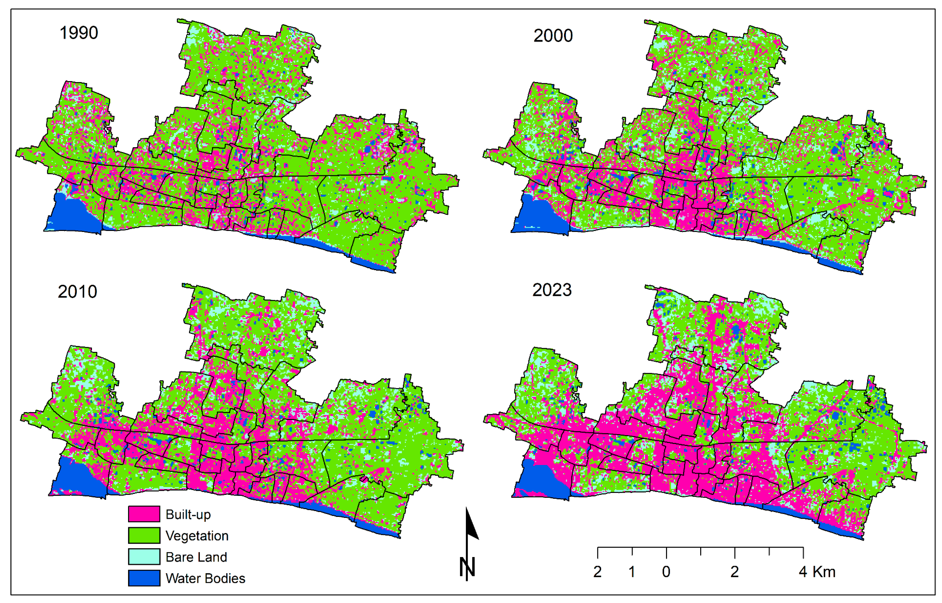
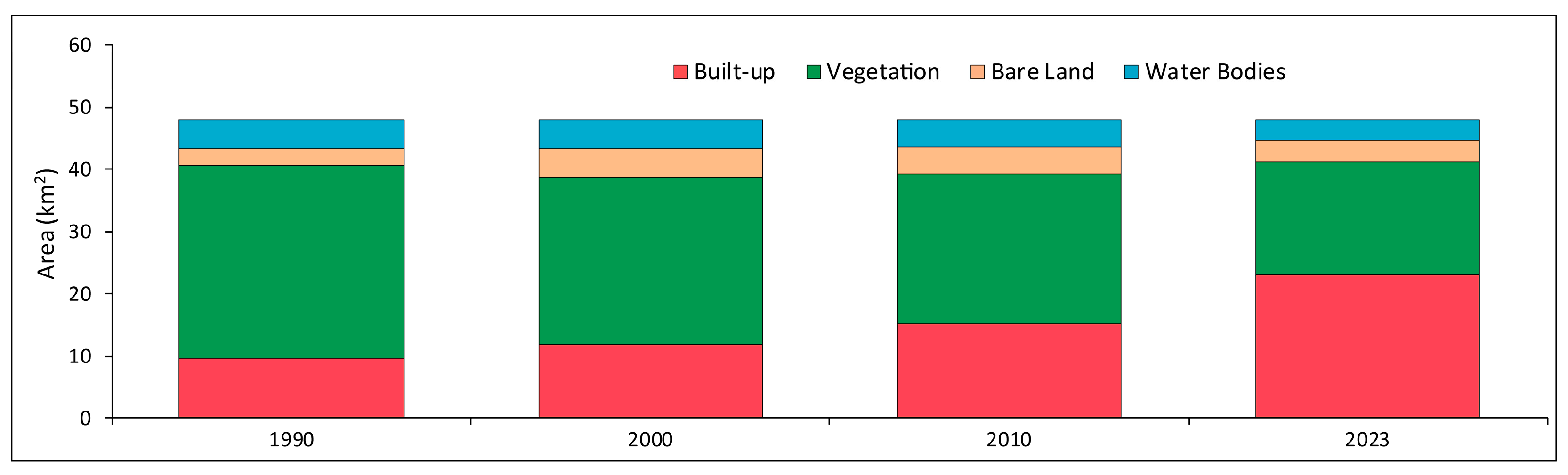
3.1. Land Use/Land Cover (LULC): Pattern and Changes

Figure 2 and Figure 3 illustrate the spatial distribution and temporal changes in LULC patterns over the study period. From Figure 2, it is evident that the most significant expansion of built-up areas occurred in the central, northern, central-western, south-eastern, and southern parts of the study area. The statistical analysis presented in Figure 3 indicates substantial LULC changes between 1990 and 2023. During this period, built-up areas expanded markedly from 9.73 km² to 22.99 km², reflecting rapid urban growth. In contrast, vegetation cover experienced a notable decline of 12.48 km², indicating a shift from natural to developed land uses. Bare land showed minor fluctuations in area, with a slight overall increase of 0.66 km², while water bodies decreased by 1.44 km², suggesting pressure on natural water resources. Overall, the built-up area increased by approximately 28%, whereas vegetated and water-covered areas decreased by 26% and 3%, respectively, over the 33-year period.

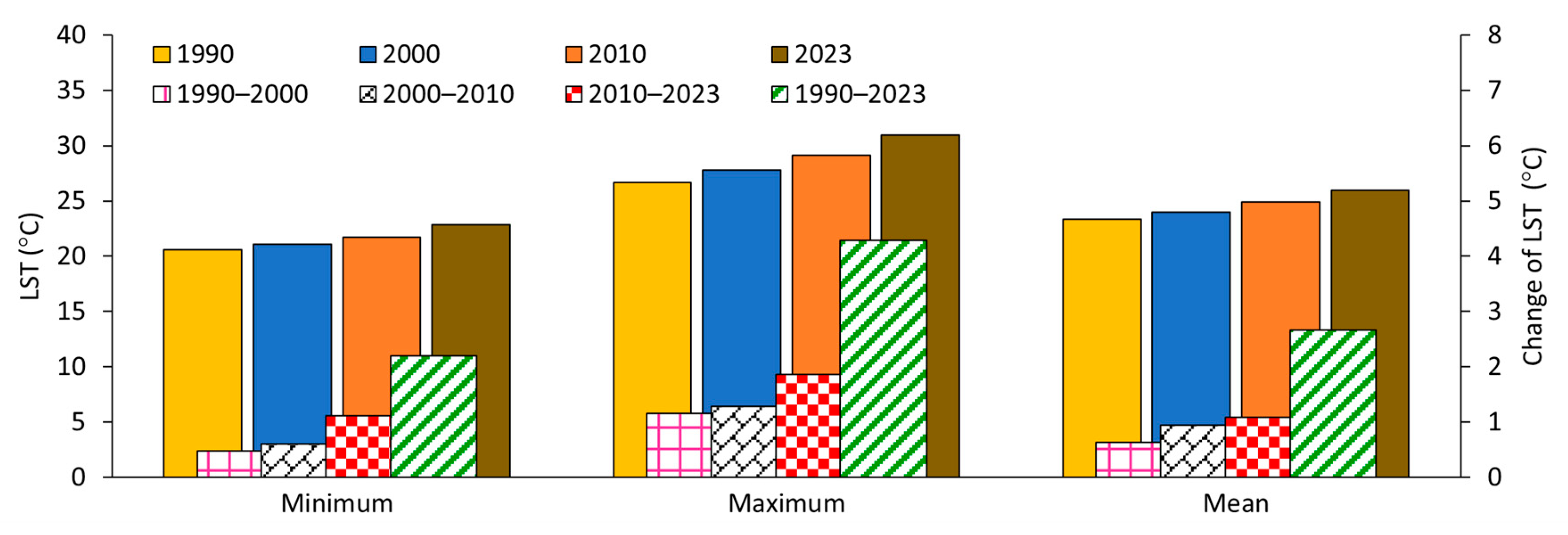
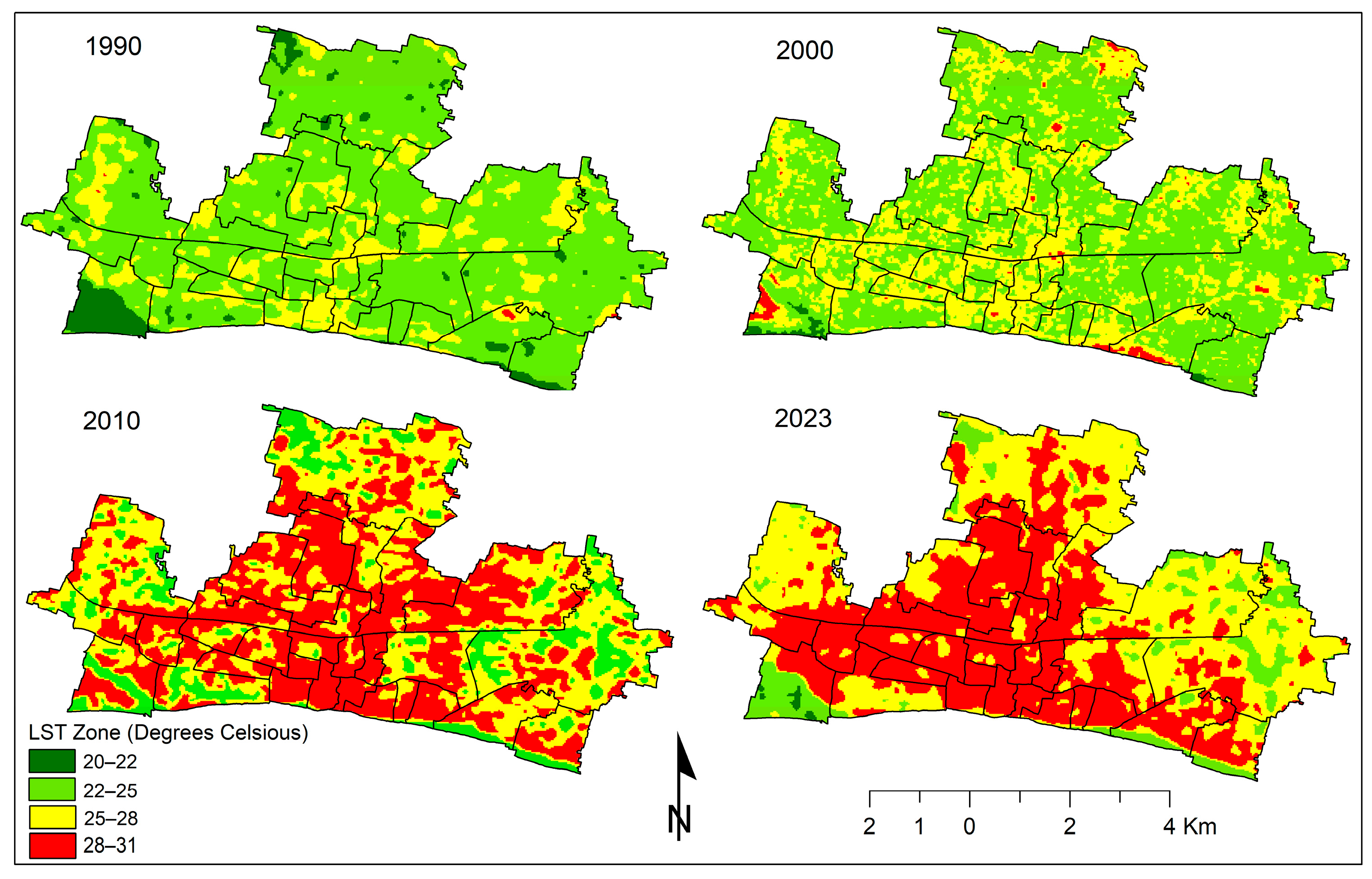
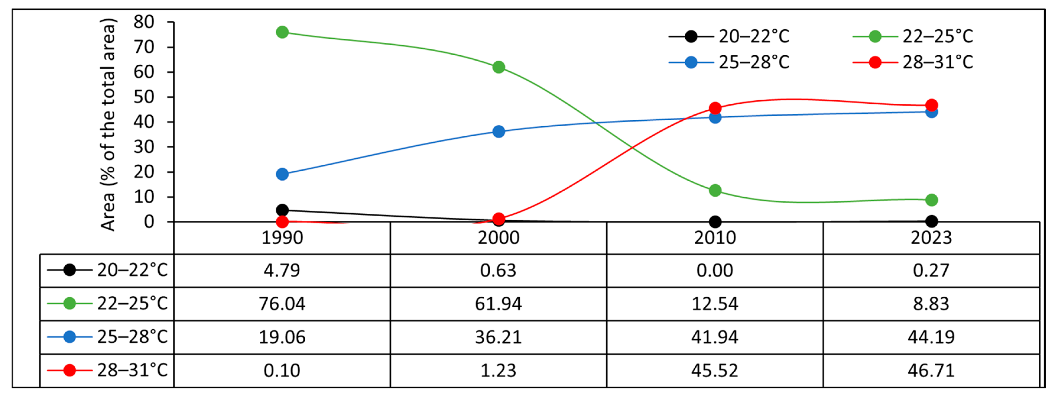
3.2. Urban Climate: LST Distribution and Dynamics

This study investigated the pattern of urban warming in the RCC area by analyzing LST using Landsat thermal imagery. Key LST metrics—including minimum, maximum, and mean values—were derived and are presented in

Table 3. Minimum, maximum, and mean LST and their changing patterns in RCC.

LST (°C)	Year				Change (°C)
	1990	2000	2010	2023	1990–2000	2000–2010	2010–2023	1990–2023
Minimum	20.62	21.10	21.70	22.82	0.48	0.60	1.12	2.20
Maximum	26.67	27.82	29.10	30.96	1.15	1.28	1.86	4.29
Mean	23.32	23.95	24.90	25.98	0.63	0.95	1.08	2.66

. The findings show a progressive rise in mean LST: from 23.32 °C in 1990 to 23.95 °C in 2000, 24.90 °C in 2010, and reaching 25.98 °C in 2023. This corresponds to mean LST increases of 0.63 °C (1990–2000), 0.95 °C (2000–2010), and 1.08 °C (2010–2023) and a total increase of 2.66 °C over the full 1990–2023 period. On average, the mean temperature rose by approximately 0.08 °C per year over these 33 years. Additionally, LST values ranged between 20.62 °C and 26.37 °C in 1990, 21.10 °C and 27.82 °C in 2000, 21.70 °C and 29.10 °C in 2010, and 22.82 °C and 30.96 °C in 2023 (Table 3 and Figure 4). Both the minimum and maximum LST values increased from 1990 to 2023. The minimum LST increased by 0.48 °C, 0.60 °C, 1.12 °C, and 2.20 °C, while the maximum LST increased by 1.15 °C, 1.28 °C, 1.86 °C, and 4.29 °C between the periods 1990–2000, 2000–2010, 2010–2023, and 1990–2023, respectively. These findings indicate a significant increase in maximum temperatures, which has contributed to the overall rise in mean temperatures in the area (Figure 4).

To analyze and interpret the spatial distribution of and temporal changes in land surface temperature (LST), we categorized LST values into four zones: 20–22 °C, 22–25 °C, 25–28 °C, and 28–31 °C (Figure 5). The spatial patterns of these zones over time reveal that the higher temperature ranges have increasingly concentrated in the central, western, and south-central parts of the city in recent decades (Figure 5). Figure 6 illustrates that from 1990 to 2023, there was a sharp change in LST distribution and levels of LST increased, particularly in the central and western parts of the city. Figure 4 denotes that in 1990 and 2000, the largest proportion of the city area, 36.50% and 29.73%, respectively, fell within the 22–25 °C LST zone. However, in 2010 and 2023, the majority of the area (20–22.50% of the total area) was within the 25–28 °C and 28–31 °C LST zones. During these years, a small proportion of the total area (≤ 6%) remained in the 20–22 °C and 22–25 °C zones. Furthermore, Figure 6 shows that the area within the 25–28 °C and 28–31 °C LST zones increased sharply from 2000 onward, while the area within the 22–25 °C zone decreased significantly during the same period. This indicates a notable shift, with a large proportion of the area originally under the 22–25 °C zone transitioning to higher-LST zones, namely, 25–28 °C and 28–31 °C.

To gain a clear understanding of the changing patterns of LST zones and the warming trend over time, the gain and loss areas of LST for each zone were analyzed between specific years. Figure 7 illustrates the conversion patterns of LST zones, highlighting areas of gain and loss. The analysis reveals a significant loss in the 22–25 °C LST zone between 1990–2000 and 2000–2010, accounting for 23.33% (11.20 km²) and 52.33% (25.12 km²) of the total area, respectively. In contrast, there was a notable increase in the areas of the 25–28 °C and 28–31 °C LST zones during 2000–2010 and 2010–2023, representing 75.40% (35.19 km²) and 34.75% (16.68 km²) of the total area, respectively. Overall, from 1990 to 2023, a large portion of the area under the 22–25 °C LST zone decreased by 71.25% (34.20 km²), while the areas under the 25–28 °C and 28–31 °C LST zones increased significantly, covering 83.10% (39.89 km²) of the total area. During this period, LST increased in about 87% of the total area. These findings indicate an overall warming trend in the urban area, primarily due to the transformation of low-LST zones to higher-LST zones (Figure 7).

To determine the level of LST increase and the spatial pattern of warming in the area, the spatial distribution of increasing LST patterns was analyzed, and the results are shown in Figure 8 and

Table 4. Spatial increasing patterns of LST.

Increase in LST (°C)	1990–2000		2000–2010		2010–2023		1990–2023
	Area (km2)	%	Area (km2)	%	Area (km2)	%	Area (km2)	%
<1	33.67	70.15	3.95	8.23	43.35	90.31	9.62	20.04
1–2	12.40	25.83	19.44	40.50	4.53	9.44	17.03	35.48
2–3	1.25	2.60	21.08	43.92	0.04	0.08	16.80	35.00
>3	0.68	1.42	3.53	7.35	0.08	0.17	4.55	9.48
Total	48.00	100.00	48.00	100.00	48.00	100.00	48.00	100.00

. Table 4 shows that during 1990–2000, most of the area (70.15%) experienced an increase of less than 1 °C, while another 25.83% of the area saw a 1–2 °C increase in LST. The spatial distribution of LST increases during this period exhibited a pepper-and-salt pattern, indicating an insignificant warming trend (Figure 8). In contrast, a significant change in LST increase was observed between 2000 and 2010. During this period, 40.50% and 43.92% of the total area experienced a 1–2 °C and 2–3 °C increase in LST, respectively, and 7.35% of the total area saw an increase of more than 3 °C. These statistics indicate that from 2000 to 2010, LST increased by 1–3 °C in about 84.42% of the total area, with some areas experiencing an increase of more than 3 °C (Table 4). The spatial pattern of LST increase reveals that areas with a 2–3 °C and more than 3 °C increase were concentrated in the central, north-eastern, and northern parts of the city, while areas with a 1–2 °C increase were spread throughout the city (Figure 8). On the other hand, during 2010–2023, a much smaller increase in LST was observed, with about 90.31% of the total area experiencing an increase of less than 1 °C and 9.44% of the area seeing a 1–2 °C increase. The slower increase in LST from 2010 to 2023, compared to the 2000–2010 period, can be attributed to changes in land use and urbanization patterns. During 2010–2023, vegetation and water bodies in the fringe areas of the city were gradually converted into paved surfaces. However, these fringe areas exhibited less compact urban development, characterized by lower building density and more open spaces. This less intensive urbanization likely mitigated the rate of LST increase, as the sparse development allowed for better heat dissipation compared to the rapid and dense urbanization observed in the earlier period. The analysis of the increasing pattern of LST between 1990 and 2023 reveals a concerning trend. Over the past 33 years, urban land surface temperature increased by 1–3 °C in 70.48% of the total area, with 9.48% of the total area experiencing an increase of more than 3 °C. The spatial distribution of LST increase from 1990 to 2023 clearly highlights that the central-northern, central part of the western zone, and south-eastern parts of the city experienced an increase of more than 3 °C. Meanwhile, the central, northern, western, and central-southern parts of the city experienced a 2–3 °C increase in LST (Figure 8). These findings indicate a dramatic increase in LST over the past three decades, with a particularly significant rise observed during 2000–2010 in the city area.

To analyze the micro-level urban climate, particularly the distribution and dynamics of urban LST, we examined the LST distribution at the Ward level, which is the basic urban administrative unit of the city. This analysis included the minimum, maximum, mean, and the range (minimum–maximum difference) of LST. The Ward-wise LST distribution showed fluctuations; however, in 1990 and 2000, both minimum and maximum LST were relatively steady. In contrast, a sharp increase in both minimum and maximum LST was observed across all wards in 2010 and 2023 (Figure 9). The average LST distribution in each ward also indicated a continuous increase in LST over the study period (Figure 9c). Figure 9a,b further reveal that the highest increases in minimum temperature occurred in Wards 20, 21, and 22, while the highest increases in maximum temperature were observed in Wards 4, 19, and 26. Conversely, the lowest minimum LST levels were found in Wards 4, 7, 25, 28, and 29, and the lowest maximum LST levels were in Wards 1, 5, 6, 8, 11, 24, and 29 (Figure 9a,b). The differences between minimum and maximum LST showed the following variations: 1.73 to 5.61 in 1990, 2.53 to 7.53 in 2000, 1.82 to 9.26 in 2010, and 1.69 to 5.52 in 2023. Both the lowest and highest variations decreased over time, and a low variation between minimum and maximum LST was observed in most wards, particularly those that are located in the central parts of the city (Figure 9d). This reflects thermal discomfort in these areas. The primary cause of these changes is the reduction in green and blue spaces due to uncontrolled and unplanned urban growth. As urban expansion extended outward from the city center, green and blue spaces in the urban fringe areas continually decreased. To improve the city’s climatic conditions, proper city planning and the implementation of greening policies are essential. These measures should aim to increase green areas or at least maintain them at steady levels for better urban climate management.

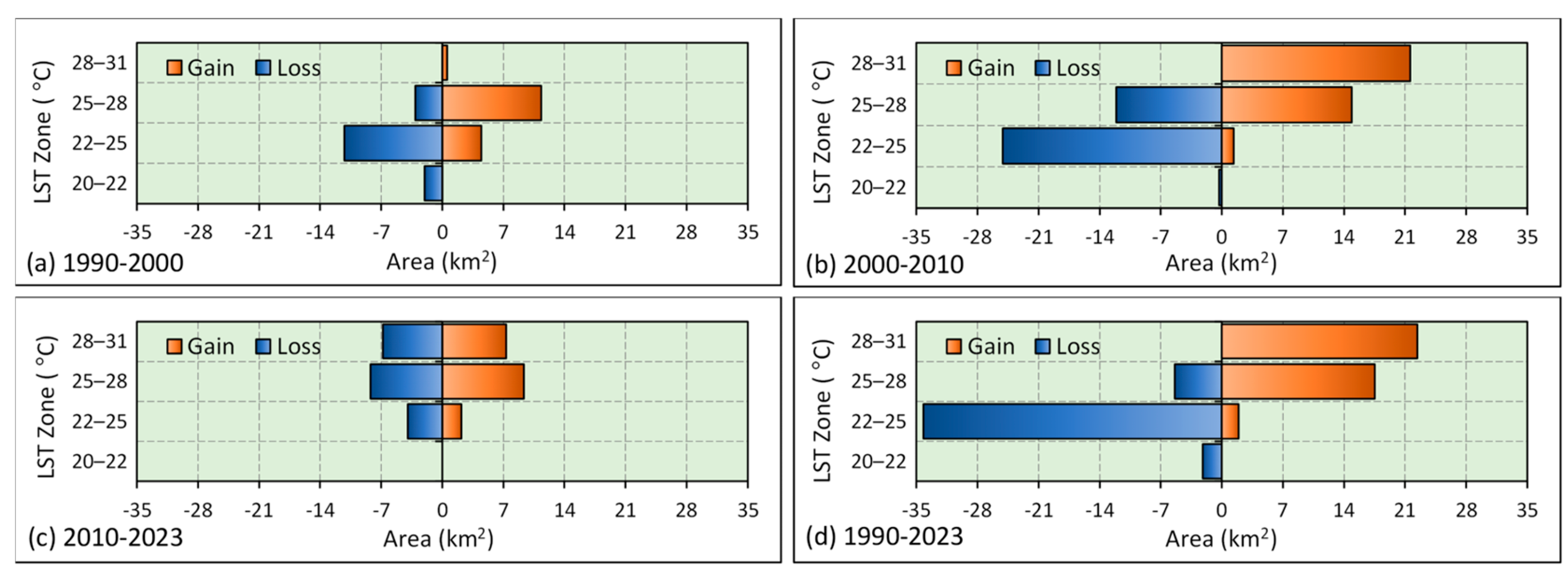
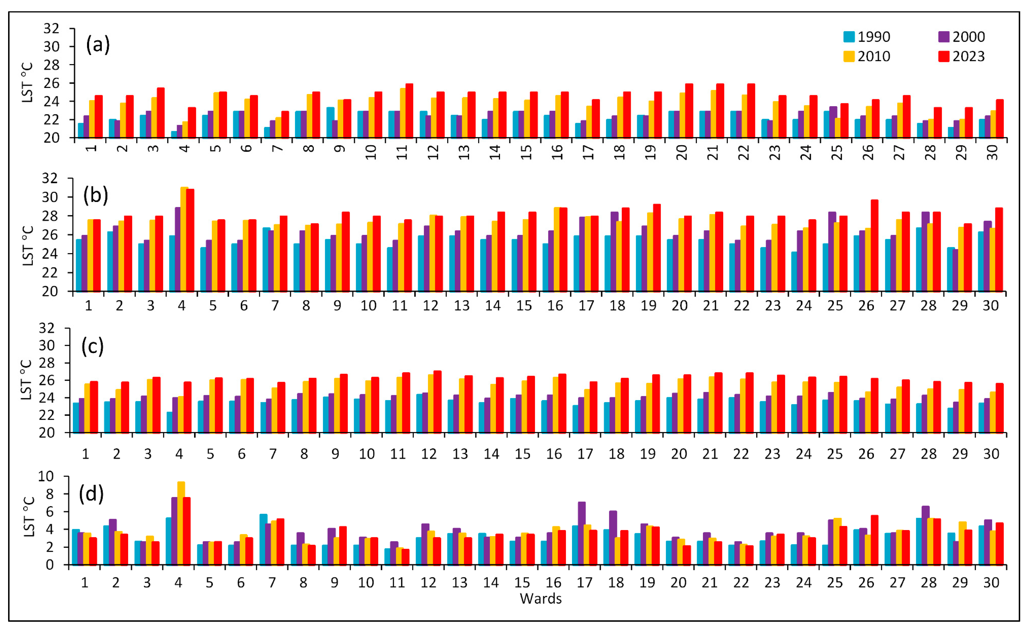
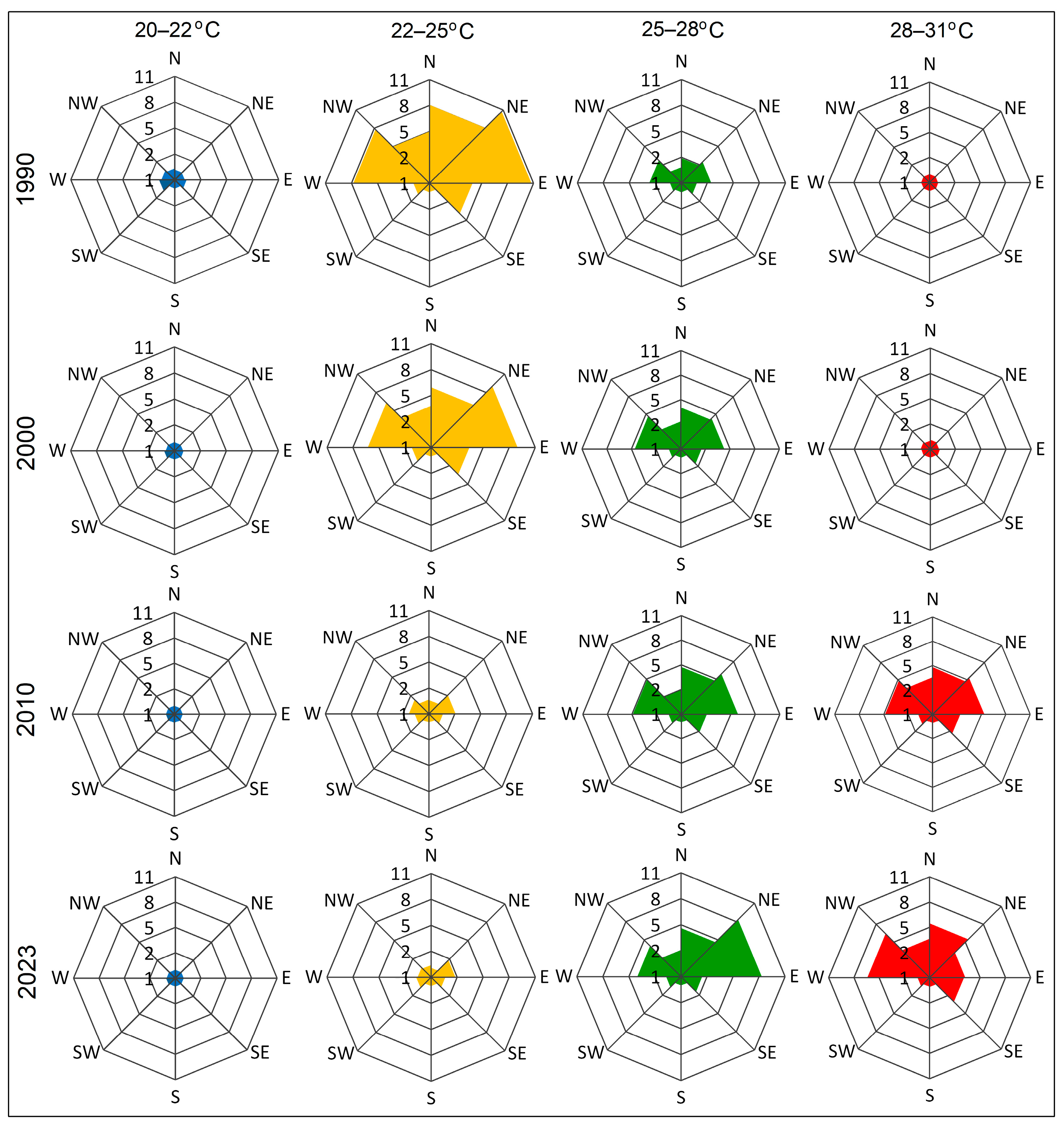
3.3. Zonal and Directional Analysis of LST

To determine the zonal and directional changes in LST, a combined directional and zonal study was conducted. This study analyzed LST changes across different LST zones by considering eight quadrants, each at a 45° angle from the city center, serving as the reference point for directional analysis (Figure 10). This combined zonal and directional analysis measures the directional change in LST zones, helping to establish spatial relationships between the LST zones and their dynamics relative to the city center [91]. Over the last 33 years, the highest area reduction in the 22–25 °C LST zone was observed in the NEE direction at a rate of 27.12 ha y⁻¹. From 1990 to 2023, the second and third highest area reductions were found in the NNE and NWW directions, at rates of 24.27 and 21.97 ha y⁻¹, respectively, for the 22–25 °C LST zone. A significant reduction in the area of the 22–25 °C LST zone was also found towards the SEE direction during this period (Figure 10). In contrast, from 1990 to 2023 the highest area increase was noted in the NWW and NNE parts of the city at rates of 19.39 and 16.58 ha y⁻¹, respectively, for the 28–31 °C LST zone. The NEE direction saw an increase of 17.70 ha per year for the 25–28 °C LST zone during the period 1990–2023 (Figure 10). A remarkable increase in the 28–31 °C LST zone was also observed in the NNW direction at a rate of 11.06 ha y⁻¹.

Figure 10 further reveals that between 1990 and 2000, the highest proportion of the city area was under the 22–25 °C LST zone, predominantly in the NEE, NNE, NWW, and NNW directions. By 2010 and 2023, an insignificant amount of the area remained under the 22–25 °C LST zone in all directions from the city center. Conversely, the area under the 25–28 °C LST zone increased gradually from 1990 to 2023, with a higher rate of increase in the NEE, NNE, and NWW directions, particularly in 2010 and 2023. The 28–31 °C LST zone (the warmest zone) saw a notable increase only in 2010 and 2023, concentrated in all directions from the city center except the south and south-west. The mighty river Padma, flowing in the southern part of the city, acted as a barrier to urban expansion, resulting in a lower increase in LST in this region. The directional analysis indicates that areas with low-LST zones, particularly the 22–25 °C range, were converted to higher-LST zones (25–28 °C and 28–31 °C) from 1990 to 2023. This conversion began primarily around 2000, with significant increases observed in 2010 and 2023. Notably, substantial growth in areas with higher LST was seen in the north, north-east, north-west, and south-east directions of the study region (Figure 10). These findings indicate the warming of the urban climate in the study area, primarily in recent decades. Rapid urban expansion, suitable land for settlement, an increase in road networks and infrastructure development, rising land values, and rapid population growth have exerted tremendous pressure on the city area, facilitating mobility and urban expansion and causing an increase in LST.

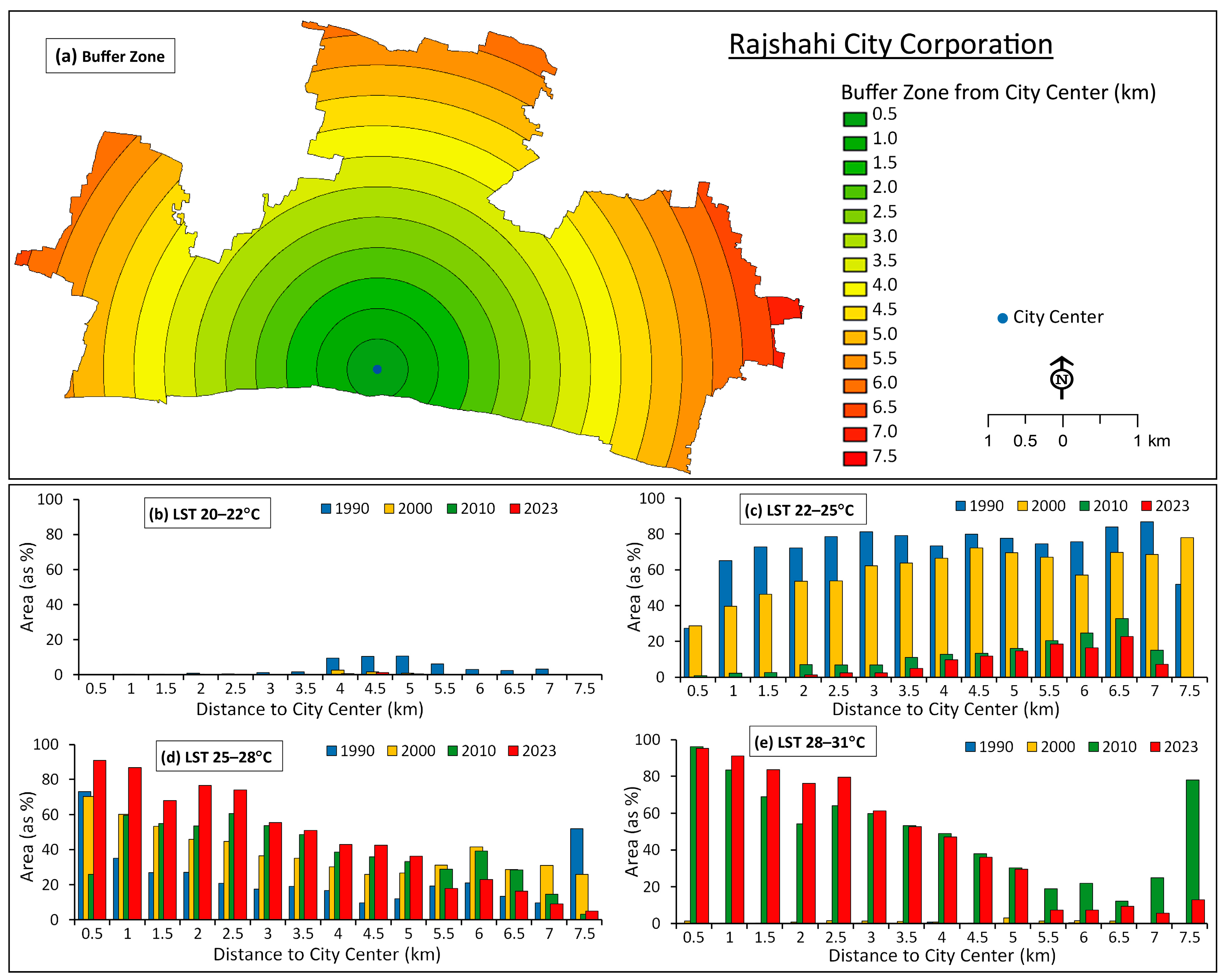
3.4. Urban–Rural Gradient of LST

The urban–rural gradient approach is utilized to examine the spatio-temporal variation of environmental variables in relation to distance within a city [85,92]. This gradient encompasses a range of conditions and characteristics, transitioning from highly concentrated urban hubs to low-density rural regions, including variations in population density, infrastructure development, economic activities, lifestyles, and environmental conditions. In this study, we apply this approach to analyze the spatial dynamics of LST at specific intervals from the city center to the rural periphery, investigating how it changes across the urban landscape [92]. The urban–rural gradient for LST shows how surface temperatures vary from urban center to rural peripheries. Urban areas, characterized by dense infrastructure, concrete, and asphalt, tend to have higher LST because of the urban heat island effect. This effect occurs due to buildings and roads absorbing and retaining heat, less vegetation, and more human activities, leading to higher daytime temperatures than in rural areas. As you move along the gradient towards suburban and rural areas, the LST gradually decreases.

To determine the pattern of LST concerning the urban–rural gradient, we measured and analyzed the areas within different LST zones using 0.5 km interval buffer zones from the city center (Figure 11a). We examined changes in the areas under various LST zones across the urban–rural gradient for the years 1990, 2000, 2010, and 2023. The results are presented in Figure 11b–e. The figure shows that the area distribution under the 20–22 °C LST zone (cooler zone) was relative to the distance from the city center, and in all the selected study years, less than 11% of each buffer area fell within this zone, with no specific pattern (Figure 11b). For the 22–25 °C LST zone, in 1990 and 2000, the area was relatively small near the city center and gradually increased towards the city periphery. However, in 2010 and 2023, both near the city center and farther from it, very small proportions of each buffer area were under this LST zone (Figure 11c). Overall, the urban–rural gradient pattern of the area under the 22–25 °C LST zone indicates that it was more dominant in 1990 and 2000, whereas in 2010 and 2023, very small areas were under this LST zone near the city center (Figure 11c). The distribution of area under the LST zones 25–28 °C and 28–31 °C from the city center to the periphery clearly shows that in 2010 and 2023, the areas dramatically increased (occupying about 60–90% of each buffer zone area) near the city center compared to the periphery (Figure 11d,e). Interestingly, for the area distribution of the 28–31 °C LST zone, in 1990 and 2000, very negligible areas were under this zone throughout the city center to the periphery. However, in 2010 and 2023, a significant amount of area fell under this zone near the city (Figure 11e). These patterns likely represent the expansion of built-up areas in the city’s core and the greater presence of vegetation near its outskirts.

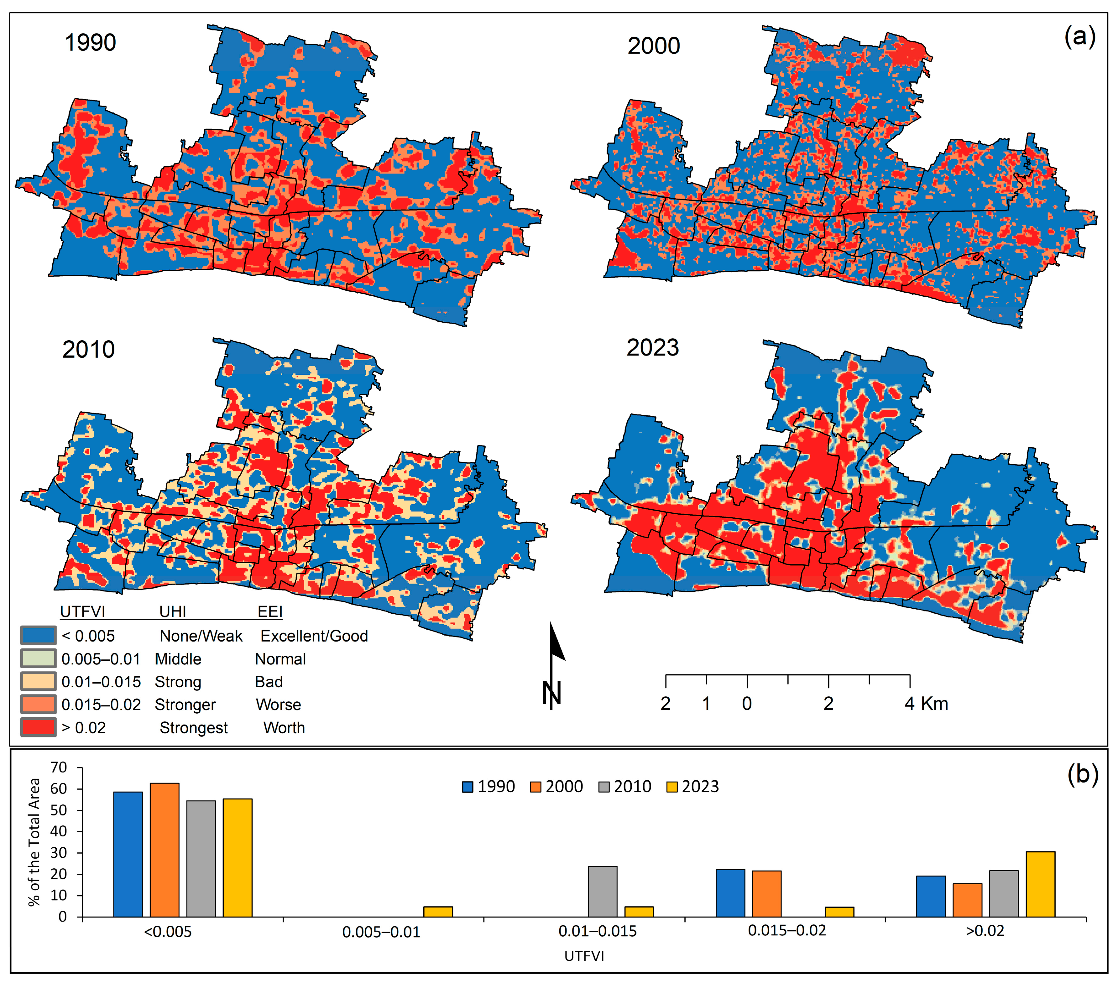
3.5. Spatio-Temporal Variation of Surface Urban Heat Island Intensity Using UTFVI

The Urban Thermal Field Variance Index (UTFVI) is a measure used to assess the intensity and distribution of urban heat islands (UHIs) within a city. It evaluates the variation in land surface temperature (LST) to identify areas with notable thermal anomalies, typically caused by dense infrastructure, limited vegetation, and high levels of human activity. By calculating the UTFVI, researchers can identify hotspots of warming, which are often associated with negative environmental and health impacts. With the increasing effects of climate change, the UTFVI becomes even more important as cities are likely to face more intense and frequent heatwaves, making it crucial to understand and mitigate UHI effects.

In this study, the UTFVI was derived from LST data, classified, and analyzed to quantitatively explain the UHI effect in the study area. A classified UTFVI offers a clear spatio-temporal indication of the condition of environment and thermal comfort in the city (Figure 12). Figure 12a illustrates the spatial pattern of UTFVI distribution in the RCC area over four different years from 1990 to 2023. The study detected changes in UHI intensity over the years, corresponding with the evolution of several thermal comfort categories in the region. By analyzing the UTFVI, it was found that 58.56%, 62.67%, 54.48%, and 55.35% of the total area in 1990, 2000, 2010, and 2023, respectively, fell under the none/weak level of UHI and good/excellent level of ecological condition, indicating these areas as thermal comfort zones (

Table 5. UTFVI, UHI phenomenon, and ecological conditions.

UTFVI	Area (km2)				% of the Total Area				Urban Heat Island Phenomenon (UHI)	Ecological Evaluation Index (EEI)
	1990	2000	2010	2023	1990	2000	2010	2023
≤0.005	28.11	30.09	26.15	26.57	58.56	62.67	54.48	55.35	None/Weak	Excellent/Good
0.005–0.01	-	-	-	2.27	-	-	-	4.73	Middle	Normal
0.01–0.015	-	-	11.40	2.24	-	-	23.75	4.67	Strong	Bad
0.015–0.02	10.69	10.39	-	2.22	22.27	21.65	-	4.63	Stronger	Worse
≥0.02	9.20	7.53	10.44	14.70	19.17	15.69	21.77	30.63	Strongest	Worst
Total	48	48	48	48	100	100	100	100	-	-

and Figure 12b). In all analyzed years, the area under the middle and strong levels of UHI, corresponding to normal and poor ecological conditions, was very low. However, in 2010 and 2023, the area under the stronger and strongest levels of UHI, indicating worse ecological conditions, showed an increasing trend, with the notably worst condition observed in 2023. This highlights a thermal discomfort zone affected by heat stress in 2023 (Table 5 and Figure 12b). Over the past 33 years, 11.46% of the city area has transitioned into the strongest level of UHI, reflecting a significantly worse ecological condition compared to the strongest UHI level in 1990. Moreover, the evolving pattern of the UTFVI reveals a warming trend in the city, especially in the central, central-western, and central-northern regions (Figure 12a). This trend correlates with increased urban development, particularly the expansion of paved areas, resulting in these regions becoming increasingly unfavorable due to heightened thermal discomfort.

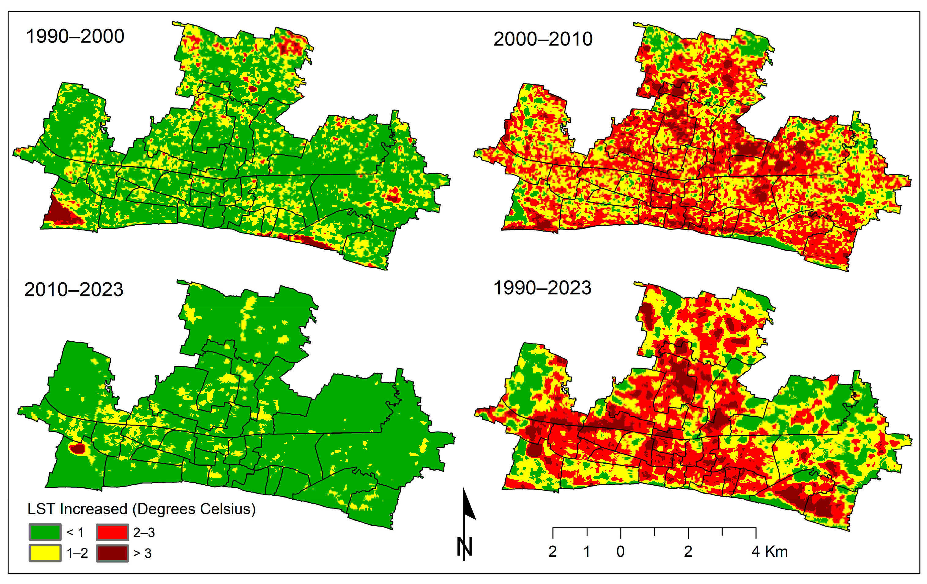
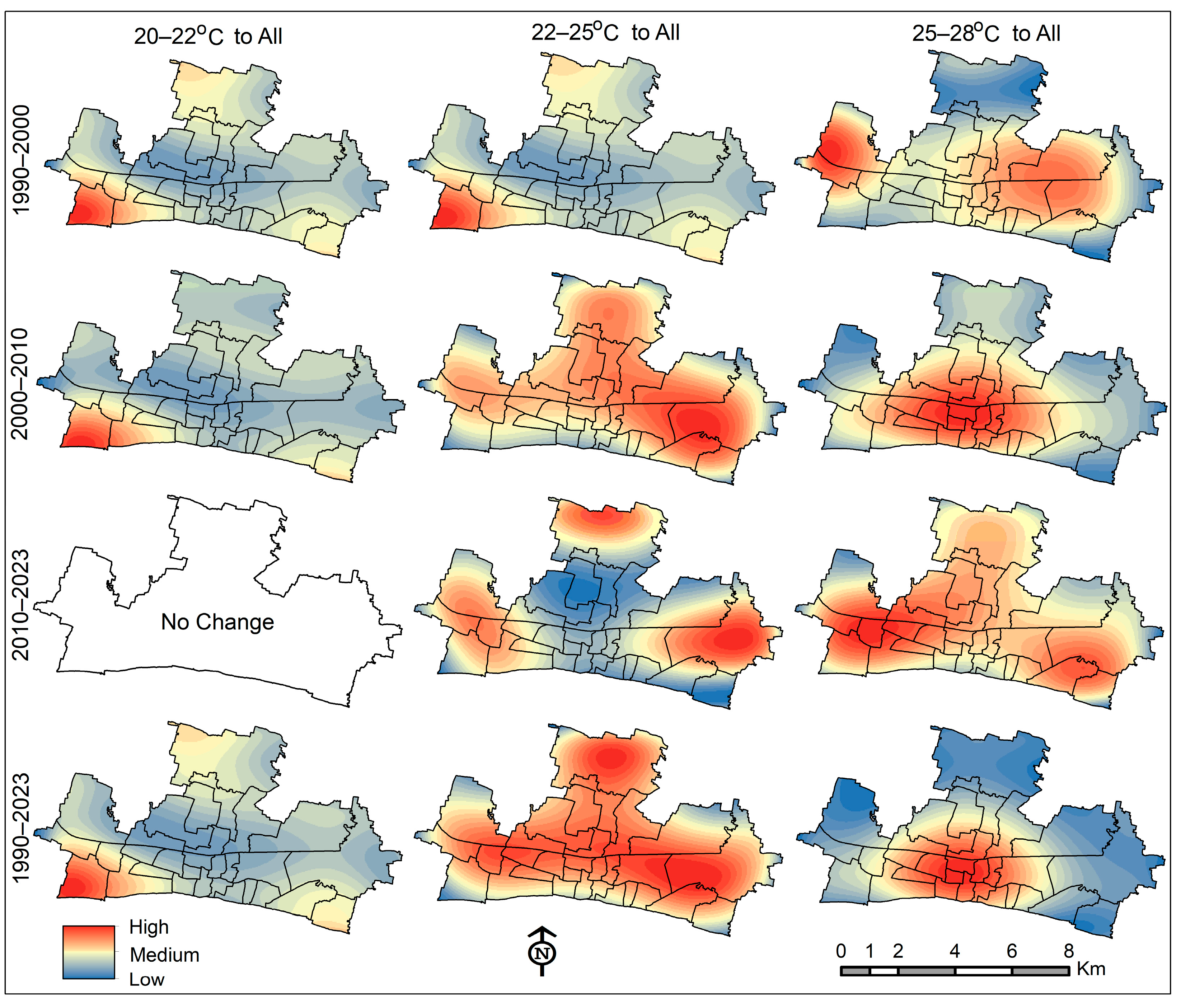
3.6. Spatial Trend of LST Change

This analysis examines the spatial trends in land surface temperature (LST) changes across different zones from 1990 to 2023. The periods analyzed include 1990–2000, 2000–2010, 2010–2023, and the entire period from 1990 to 2023. The spatial trend analysis, as depicted in Figure 13, provides insight into the patterns of temperature changes and simplifies the trend of these changes [93]. During these periods, the changes in LST from 20–22 °C to other levels were generally not significant, with trends mostly ranging from low to medium (Figure 13). In contrast, the trends in LST changes from 22–25 °C to other levels were more pronounced. From 1990 to 2000 and 2000 to 2010, significant increases were observed, especially in the central, northern, central-western, and eastern parts of the city. This trend continued from 2010 to 2023, extending notably towards the northern, eastern, and western areas of the city. Over the entire period from 1990 to 2023, the spatial pattern of LST changes from 22–25 °C to other levels indicated that temperature increases predominantly occurred in the central, western, northern, and south-eastern parts of the city. The increase in LST began in the central areas and gradually spread towards the western, northern, and eastern regions (Figure 13).

For LST changes from 25–28 °C to other levels, high trends were observed in the central-eastern and western parts of the city from 1990 to 2000. In the period from 2000 to 2010, this high trend was concentrated in the central part of the city (Figure 13). However, from 2010 to 2023, the high changing trends were primarily located in the south-eastern and south-western parts of the city. Overall, from 1990 to 2023, the most extreme LST increases were concentrated in the central part of the city (Figure 13). Finally, the trend analysis of LST zones reveals that the central, northern, western, and south-eastern parts of the city have experienced significant increases in LST, making them more vulnerable in terms of eco-urban structure and urban thermal comfort. This vulnerability is largely due to urban development, the reduction in vegetation, and the loss of water bodies in these areas. For sustainable urban development and improved urban thermal comfort, it is crucial to prioritize these areas for restoration efforts. This includes reintroducing greenery, protecting existing green and blue spaces, and possibly expanding water bodies to mitigate the effects of rising land surface temperatures.

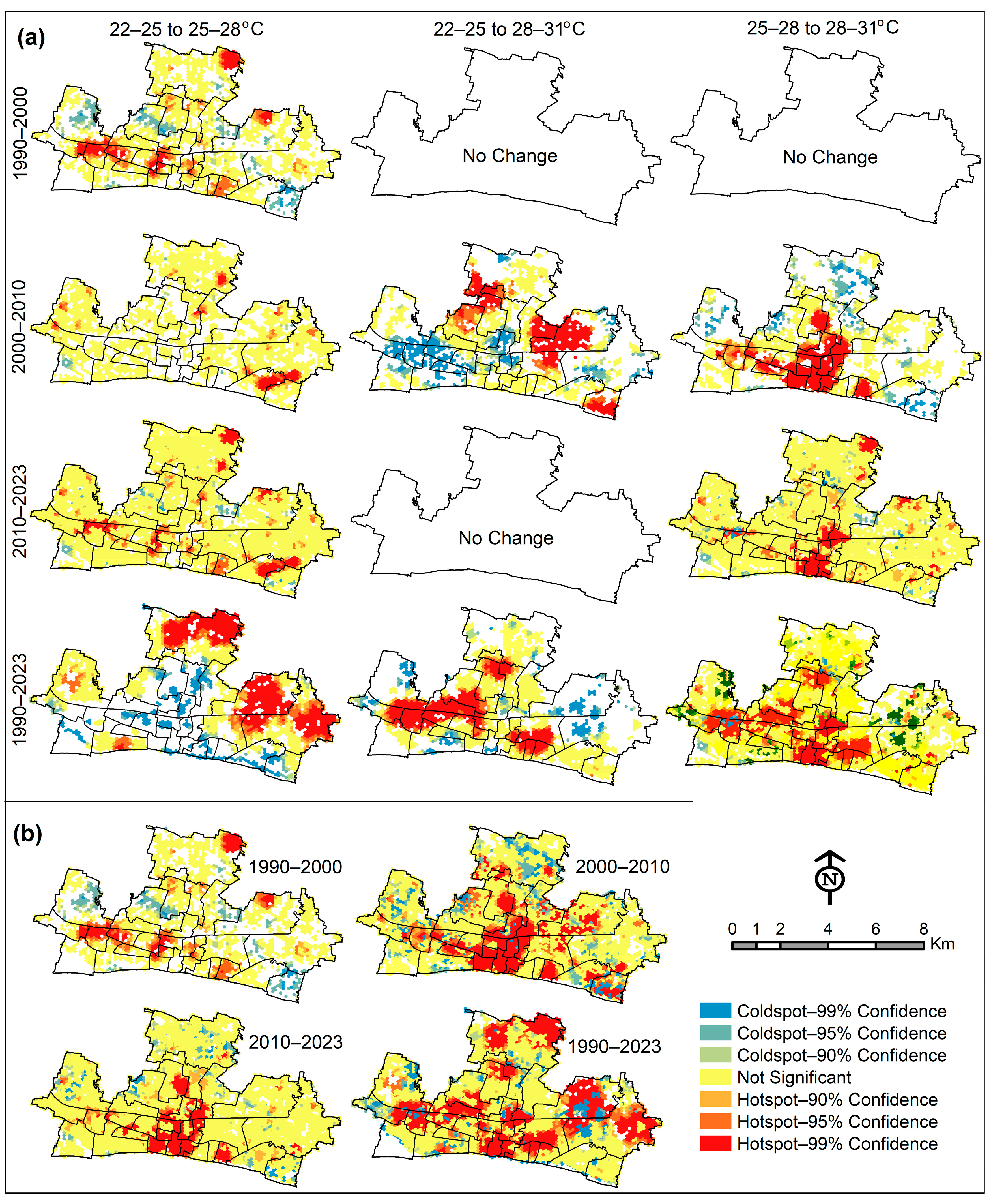
3.7. Hotspot Analysis of LST Change

To identify significant hotspots of LST changes across different zones, a hotspot analysis was executed using Getis-Ord Gi* (G-i-star) statistics. Specifically, we analyzed hotspots for the changes in LST zones of 22–25 °C to 25–28 °C, 22–25 °C to 28–31 °C, and 25–28 °C to 28–31 °C. As shown in Figure 14, for the LST change from 22–25 °C to 25–28 °C, hotspots with a 99% confidence level were observed sparsely distributed across the city, with only a few patches identified during the periods 1990–2000, 2000–2010, and 2010–2023. Overall, significant hotspots for this LST change during 1990–2023 were mainly distributed in the northern and north-eastern parts of the city (Figure 14a). During 2000–2010, hotspots for the LST change from 22–25 °C to 28–31 °C were predominantly observed in the north-western and north-eastern parts of the city. For the extreme LST change from 25–28 °C to 28–31 °C, hotspots with a 99% confidence level were concentrated in the central, central-southern, and, to some extent, central-western parts of the city (Figure 14a). In addition to analyzing the zonal distribution of LST hotspots, we also examined the hotspots based on all LST zones combined. The observed spatial patterns of LST change hotspots are presented in Figure 14b. The figure illustrates the evolving pattern of these hotspots over time. From 1990 to 2000, only a few significant hotspot patches were identified. However, during 2000–2010 and 2010–2023, significant LST change hotspots became more concentrated in the central, central-southern, and central-northern parts of the city. Considering the entire period from 1990 to 2023, significant hotspot areas of LST change were identified as compact patches in the central, eastern, northern, and central-western parts of the city (Figure 14b). This indicates significant warming in these areas over time.

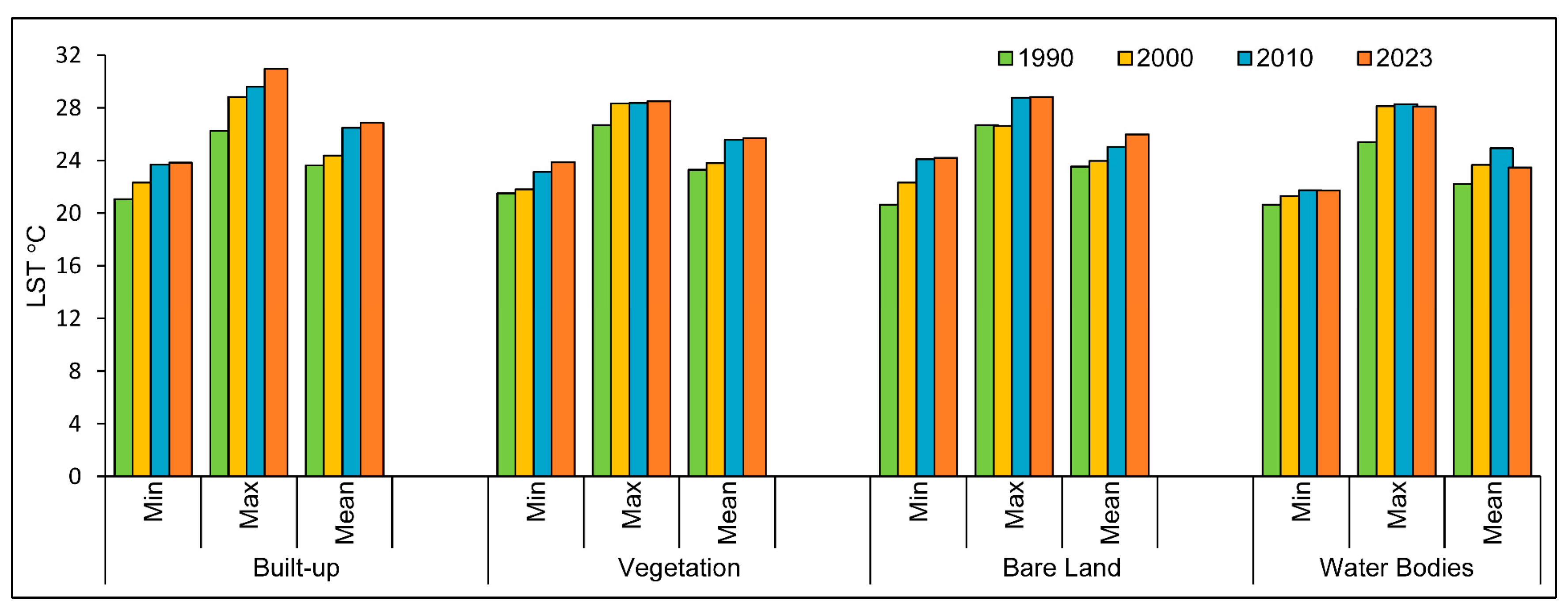
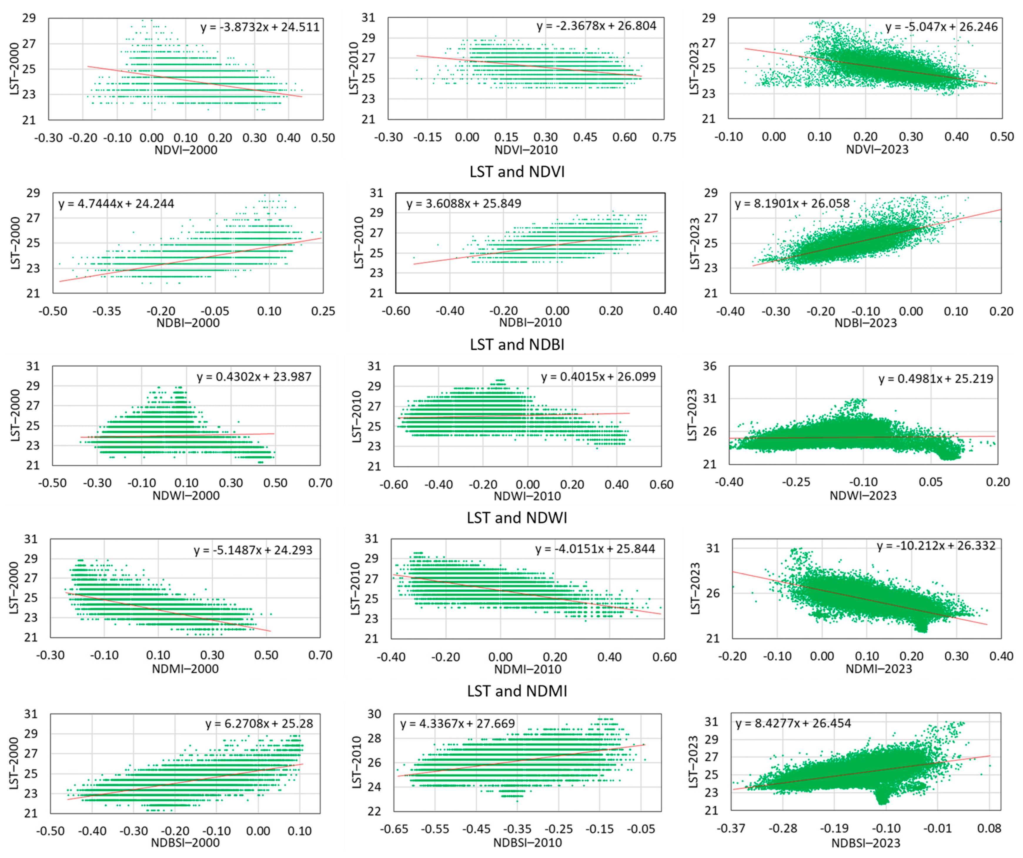
3.8. Relationship Between LST, LULC, and Biophysical Component

While the analysis of LST changes, trends, and hotspots provides valuable insights, understanding the relationship between LST variations, LULC, and key biophysical urban components is crucial for identifying the drivers of LST increase. In urban areas, the spatial dynamics of LST are strongly influenced by the eco-environment and landscape structure. Major factors affecting LST include the extent of built-up areas, vegetation cover, presence of water bodies, bare soil exposure, and soil moisture levels. To explore these relationships, we analyzed the spatial patterns of LST increase alongside LULC distribution (Figure 15) and conducted correlation and regression analyses to examine the associations between LST and several critical biophysical variables (Figure 16). Figure 15 reveals that LST is highest in built-up and bare land areas and has increased more rapidly in these zones compared to vegetated regions and water bodies. The expansion of built-up areas between 1990 and 2023 (Figure 3) significantly contributed to local warming, with average surface temperatures rising from 23.64 °C to 26.85 °C, an increase of 3.21 °C. A significant portion of this rise (2.43 °C) is linked to the loss of vegetation cover, which formerly helped moderate surface temperatures. The reduction in water bodies during this period also contributed to a smaller but notable increase of 1.25 °C. Overall, the study period saw an average surface temperature rise of 2.66 °C, highlighting the substantial impact of urbanization and LULC changes on the local climate. On the other hand, Figure 16 illustrates a strong positive correlation between LST and both the NDBI and the NDBSI, indicating that built-up areas and bare soil are major contributors to elevated surface temperatures. In contrast, LST shows a significant negative correlation with the NDVI and the NDMI, reflecting the cooling effects of vegetation and soil moisture. An insignificant positive relationship is observed between LST and the NDWI. These findings emphasize that low levels of vegetation, soil moisture, and surface water, combined with high proportions of impervious surfaces and exposed soil, substantially contribute to LST increases. In essence, areas lacking greenery, moisture, and water exhibit higher surface temperatures, and ongoing declines in these components exacerbate the warming trend. Conversely, the expansion of built-up and bare areas correlates strongly with higher LST, reinforcing the role of urbanization and landscape transformation in driving local temperature increases.

4. Discussion

Land surface temperature is an important phenomenon, with its dynamics playing a strong role in understanding urban climate patterns and the impacts of urbanization. The findings contribute meaningful understanding into the winter LST dynamics in Rajshahi City, Bangladesh, using Landsat data and GIS technology for the years 1990, 2000, 2010, and 2023. The findings indicate that LST has shown a marked increase during the 33-year study period, with the mean LST rising by approximately 2.66 °C (0.08 °C per year) from 1990 to 2023. Specifically, the minimum and maximum LST increased by 2.20 °C and 4.29 °C, respectively, during this period, highlighting a pronounced trend in the maximum LST increase during the study period. This indicates a faster warming of the LST in the city, primarily due to the noticeable rise in maximum LST over the past three decades. Similar trends, i.e., rises in LST, have been observed in various South Asian cities and other parts of the world [24,51,58,75,85,94,95]. For instance, studies have shown significant LST increases in cities such as Dhaka and Chattogram in Bangladesh. In Dhaka, the mean LST increased by about 7.6 °C from 1989 to 2009 [51], while in Chattogram, Ref. [75] reported a 9.60 °C increase in mean LST over the last 30 years. Ref. [50] also found a 6.5 °C increase in mean LST in Chattogram during the period 1998–2018. In Bogra, the mean LST increased by 0.62 °C from 2001 to 2020 [49], and in Khulna, the mean LST rose by 5.54 °C in urban areas and 4.14 °C in suburban areas during the period 1998–2018 [96]. The variation in LST increases across different cities can be attributed to regional weather patterns, levels of urban development, population growth rates, and land use patterns. However, all these studies consistently indicate an overall increase in LST in urban areas over time. Moreover, similar findings of LST increases have been reported in other parts of the world [21,37,78,92], underscoring the global relevance of this issue. This study’s results align with these broader trends, emphasizing the need for further research and policy measures to address the impacts of rising LST in urban environments. Moreover, the 2.66 °C rise in temperature over 33 years (0.80 per decade) is significantly higher than the global average increase of about 0.2–0.3 °C per decade, according to the IPCC [9]. In cities like Rajshahi, local factors such as rapid urban growth, loss of vegetation, and more paved surfaces are likely speeding up this warming. This highlights the importance of city-specific strategies to reduce the impacts.

During the study period, the spatial patterns of LST increases were analyzed in Rajshahi City. The central-northern, central part of the western zone, and south-eastern parts of the city experienced an increase of more than 3 °C. Additionally, the central, northern, western, and central-southern parts of the city experienced a 2–3 °C increase in LST (Figure 8). These dramatic increases in high-LST areas account for about 45% of the total study area, primarily due to the transformation of 22–25 °C LST zones into 25–28 °C and 28–31 °C LST zones (Figure 7), indicating an overall warming trend in the urban area. Areas experiencing winter LST increases of ≥3 °C may face significant environmental, social, and economic consequences. Such warming can alter local microclimates, reduce seasonal cooling relief, and contribute to thermal discomfort, thereby diminishing urban livability and increasing the risk of heat-related stress. According to [97], if the LST is between 27 and 29 °C, the greater part of the community in that area is expected to feel discomfort, and if it is between 29 and 31 °C, the total inhabitants are likely to feel uneasy. Therefore, the LST zones of 25–28 °C and 28–31 °C, where LST has increased by 3 °C or more, can be identified as discomfort thermal zones of the city. These areas have shifted from lower to higher risk levels over time, which correlates with the increase in the built-up area and contraction in the vegetated area. Additionally, due to similar circumstances, Wards 19, 20, 21, 22, and 26, which are primarily located in the central part, can be identified as vulnerable to rising LST and increased thermal discomfort. Particular focus should be given to these wards for effective management. Several cities across low- and middle-income countries have observed that local warming has increased due to urbanization, resulting in deteriorated urban thermal comfort alongside the rise in LST [98].

Rising temperature in urban areas is influenced by changes in LULC, particularly the expansion of built-up areas and the reduction in water bodies. In Rajshahi City, the built-up area dramatically increased from 9.73 km² in 1990 to 22.99 km² in 2023, a gain of 13.26 km² (Figure 3 and Figure 7). The most significant increases in built-up areas occurred in the central, southern, and western parts of the city (Figure 5), which correspond to areas with a 3 °C or greater rise in LST (Figure 8). Consequently, the highest LST increases were observed in the wards located in these parts of the city (Figure 9). LST distribution by LULC classes shows that LST is higher in built-up and bare land areas and has increased more rapidly compared to vegetated areas and water bodies (Figure 15). Built-up areas, dominated by impervious surfaces, absorb and emit solar radiation quickly, leading to higher temperatures [58]. In contrast, vegetation absorbs most of the solar radiation and acts as an intercepting surface, reflecting very little radiation. Water bodies have similar properties. The increase in built-up areas at the expense of vegetation and water has contributed notably to rising LST in Rajshahi. It is worth noting, however, that this analysis emphasizes surface temperatures and does not include air temperature, which also plays a key role in urban heat dynamics. Additionally, sensible heat represents only one element contributing to surface energy dynamics. The role of latent heat, which includes the effects of evaporation and transpiration, should also be considered to gain a more inclusive sense of the warming in the area. These factors present opportunities for further research and could serve as valuable directions for future studies. The highest increases in LST were observed in areas where land use changed from vegetated and water areas to built-up areas. Area under vegetation and water play a crucial role in controlling temperature in urban areas. To reduce LST, maintaining a good proportion of vegetation and water bodies is essential.

Again, zonal and directional analysis in this study reveals that low-LST zones progressively transformed into higher-LST zones over time, with significant increases observed in 2010 and 2023. Notably, higher LST was concentrated in the northern, north-eastern, north-western, and south-eastern areas of the city. This rise in LST can be attributed to rapid urban expansion and population growth in these regions. The transformation of non-urban areas into urban zones indicates that greater urbanization is closely linked to higher LST. Since the rate of urban conversion was highest near the city center, these areas experienced the most significant rise in LST over the study period. Consequently, LST gradually decreased along the gradient from the city center toward suburban and rural areas. The spatial distribution of high-LST zones from the city center to the periphery (urban–rural gradient) over time shows that the concentration of high-LST areas increased closer to the city center, particularly in recent decades. These LST patterns also reflect changes in land use, characterized by dense urban development in the city center and higher levels of vegetation in the outer zones. Both factors significantly contribute to LST distribution and urban warming. The findings from this zonal and urban–rural gradient analysis of LST changes offer valuable insights for urban planning. They can support climate resilience strategies, improve public health and urban thermal comfort, and promote the development of green infrastructure and sustainable practices to mitigate heat stress within urban areas.

In urban areas, the dynamics of LST, particularly its spatial patterns, largely depend on the urban eco-environment and landscape. The connection between LST change and biophysical urban components reveals a strong positive relationship between LST and the NDBI and the NDBSI. Conversely, an inverse relationship was found between LST and both the NDVI and the NDMI. Thus, low levels of greenery, soil moisture, and water bodies, along with high levels of impervious surfaces and bare soil, remarkably contribute to rising LST. The findings of this study and the observed associations between LST and selected biophysical components are consistent with several previous studies. For instance, Ref. [99] found a sharp increase in extremely high-temperature zones over time, largely due to the decline in agricultural lands and water bodies, which were gradually replaced by construction areas. Similarly, Ref. [47] observed that built-up areas exhibited the highest mean LST, followed by bare soil and vegetation. Ref. [100] noted significant increases in LST within urban areas, particularly in paved regions, while [101] confirmed that the expansion of built-up areas contributed to a rise in LST over time. Furthermore, Ref. [102] identified a positive correlation between NDBI, NDBSI, and LST, whereas NDVI and NDWI were inversely related to LST. This suggests that a higher presence of water bodies, healthy vegetation cover, ample open spaces, and reduced concrete surfaces are crucial for maintaining lower LST in urban environments.

Moreover, urban climate change, as reflected in the UTFVI, reveals a significant increase in urban heat island intensity as categorized by the strongest UHI over the past three decades. This UHI zone was increased by 11.46% of the total area, indicating a critical ecological deterioration and a concerning warming trend in LST, particularly in the central, central-western, and central-northern parts. These regions correspond to areas of rapid urban development, characterized by the expansion of paved surfaces, which exacerbate thermal discomfort and make these areas increasingly unfavorable for living conditions. Urbanization alters the local climate by replacing natural surfaces with impervious ones, leading to increased heat absorption and reduced evapotranspiration. This change contributes to higher local temperatures and exacerbates the UHI effect. Refs. [48,78,103,104] highlighted that the gradual increase in LST contributes to the intensification of UHI. UTFVI levels tend to be higher in areas that are significantly warmer than their surroundings. These studies also emphasized the notable impacts of elevated UTFVI, including adverse effects on local wind patterns, humidity, air quality, and overall comfort levels, which indirectly result in economic losses. Furthermore, Ref. [78] observed a mutual linkage between the UTFVI microclimate thermal zones and urban land cover patterns. Areas with vegetation cover corresponded to optimal microclimates (UTFVI < 0.01), whereas thermal discomfort zones (UTFVI > 0.01) were associated with impervious surfaces. Furthermore, through spatial trends and hotspot analysis of LST changes, we observed that over the past 33 years, LST has predominantly increased in the central, western, northern, and south-eastern parts. The rise in LST initially began in the central areas and gradually expanded towards the western, northern, and eastern regions. Significant LST hotspots during this period were identified as compact clusters in the central, eastern, northern, and central-western parts. These findings highlight remarkable warming in these areas over time, designating them as zones of heightened thermal discomfort. Therefore, proactive measures are necessary to mitigate urban heat island effects, foster sustainable urban development, and enhance the overall quality of life in urban areas.

5. Conclusions

This study examined urban climate dynamics in Rajshahi City, Bangladesh, focusing on land surface temperature (LST) changes and heat island intensity in relation to selected biophysical compositions over the period 1990 to 2023. Using Landsat thermal data and GIS techniques, LST changes were analyzed geospatially. The results revealed a significant increase in urban LST during this period, with the mean LST rising by 2.66 °C (0.08 °C per year), accompanied by increases of 2.20 °C in minimum LST and 4.29 °C in maximum LST. These findings indicate a pronounced warming trend in the urban area. The geospatial analysis highlighted that areas in the central-northern, central-western, and south-eastern parts of the city saw LST rises exceeding 3 °C, accounting for approximately 10% of the total area. while another 35% saw increases of 2–3 °C, encompassing regions in the central, northern, western, and central-southern parts. This alarming rise in LST has resulted in expanding thermal discomfort zones, posing significant environmental and public health risks. Furthermore, the observed LST increases (>2.0 °C) in these urban zones have already surpassed the United Nations Framework Convention on Climate Change (UNFCCC) aim to cap temperature increases below the 2.0 °C threshold [105]. Hence, this evidence reinforces the call for resilient urban design and heat mitigation measures to manage the growing threat of urban warming. The primary driver of this warming is rapid urban development and expansion, which has transformed areas under vegetation and water bodies into impervious surfaces, intensifying the UHI effect. This was validated by a strong positive correlation between LST and indices such as the NDBI and NDBSI and a strong negative correlation between LST and the NDVI, NDWI, and NDMI. The results highlight that reductions in green and blue spaces, coupled with expanded paved surfaces, directly contribute to increased urban temperatures. If this trend persists, further reductions in green and blue spaces, coupled with an increase in paved areas, will likely result in even greater urban warming in the future.

The spatial analysis of LST changes revealed that higher LST areas corresponded to regions of intense urbanization, with a growing concentration of high-LST zones near the city center in recent decades. This aligns with the transformation of land uses in central areas, where non-urban land has been replaced by built-up infrastructure, in contrast to the peripheral zones. The UTFVI further highlighted the expansion of strong UHI effects, spanning around a third of the urban landscape, primarily clustered in the core, central-western, and central-northern regions. The UTFVI and UHI analyses serve as vital tools for urban planners, aiding in the strategy development to mitigate LST impacts and encourage sustainable urban expansion. Moreover, hotspot analysis identified compact clusters of LST in central, eastern, northern, and central-western areas, marking zones of significant thermal discomfort and ecological vulnerability. These findings reinforce the urgent need for climate-responsive urban planning. Preserving vegetation, enhancing water bodies, promoting permeable surfaces, and adopting climate-adaptive urban design are essential for mitigating heat stress. The integration of Landsat and GIS in this study also provides a scalable framework for analyzing urban thermal patterns in other rapidly urbanizing regions. However, it is important to note that this study relied on single-date thermal satellite data due to the limited availability of consistent, high-resolution thermal imagery over extended time periods. This constraint represents a limitation of the dataset. Nevertheless, the adopted approach remains methodologically sound and is widely supported in the literature [31,100,101]. Future studies could strengthen the analysis by incorporating multi-temporal or seasonal data as they become more readily available. Finally, to mitigate UHI effects and urban warming, it is crucial to prioritize urban greening initiatives, incorporate permeable surfaces, and adopt climate-resilient urban designs. Regular monitoring of LST and UHI patterns using satellite data, along with fostering community engagement in green infrastructure projects, is essential for creating sustainable urban environments. Rajshahi City Corporation (RCC) has recently initiated the ‘Zero Soil Project’, aimed at reducing bare soil and converting it to vegetation to combat UHI impacts and improve the city’s ecological conditions. By addressing the challenges identified in this study and implementing the recommended strategies, Rajshahi City can alleviate the urbanization-induced climate stress and move toward a more resilient and sustainable cityscape. Furthermore, combating urban climate change on an international scale requires collaborative efforts to share best practices, improve technological accessibility, and promote green infrastructure globally. Policies emphasizing sustainable urban development, coupled with continuous monitoring and global knowledge exchange, can help cities worldwide adapt to and mitigate the effects of urban climate change, fostering more resilient and livable urban landscapes.

References

1. Abulibdeh, A. Analysis of urban heat island characteristics and mitigation strategies for eight arid and semi-arid gulf region cities. Environ. Earth Sci. 2021, 80, 259. [Google Scholar] [CrossRef] [PubMed]
2. Halder, B.; Bandyopadhyay, J.; Banik, P. Monitoring the effect of urban development on urban heat island based on remote sensing and geo-spatial approach in Kolkata and adjacent areas, India. Sustain. Cities Soc. 2021, 74, 103186. [Google Scholar] [CrossRef]
3. Sarif, M.O.; Ranagalage, M.; Gupta, R.; Murayama, Y. Monitoring urbanization induced surface urban cool island formation in a South Asian megacity: A case study of Bengaluru India (1989–2019). Front. Ecol. Evol. 2022, 10, 1–17. [Google Scholar] [CrossRef]
4. Kalnay, E.; Cai, M. Impact of urbanization and land-use change on climate. Nature 2003, 423, 528–531. [Google Scholar] [CrossRef]
5. Ren, G.; Zhou, Y.; Chu, Z.; Zhou, J.; Zhang, A.; Guo, J. Implications of temporal change in urban heat island intensity observed at Beijing and Wuhan stations. Geophys. Res. Lett. 2007, 34, 1–5. [Google Scholar] [CrossRef]
6. Zhou, D.; Zhang, L.; Hao, L.; Sun, G.; Liu, Y.; Zhu, C. Spatiotemporal trends of urban heat island effect along the urban development intensity gradient in China. Sci. Total Environ. 2016, 544, 617–626. [Google Scholar] [CrossRef]
7. Yang, J.; Wang, Y.; Zhang, Y.; Wang, Z. Modulation of Wintertime Canopy Urban Heat Island (CUHI) Intensity in Beijing by Synoptic Weather Pattern in Planetary Boundary Layer. J. Geophys. Res. Atmos. 2022, 127, e2021JD035988. [Google Scholar] [CrossRef]
8. Xian, G.Z. Monitoring and assessing urban heat island variations and effects in the United States. U.S. Geol. Surv. Fact Sheet 2021, 2021–3031, 2. [Google Scholar] [CrossRef]
9. IPCC. Climate Change 2021: The Physical Science Basis; Contribution of Working Group I to the Sixth Assessment Report of the Intergovernmental Panel on Climate Change; Masson-Delmotte, V., Zhai, P., Pirani, A., Connors, S.L., Péan, C., Berger, S., Caud, N., Chen, Y., Goldfarb, L., Gomis, M.I., et al., Eds.; Cambridge University Press: Cambridge, UK, 2021. [Google Scholar] [CrossRef]
10. Walsh, S. A Summary of Climate Averages for Ireland: 1981–2010. In Climatological Note 2012; No.14; Met Éireann: Dublin, Ireland, 2012. [Google Scholar]
11. Rahman, M.R.; Lateh, H. Climate change in Bangladesh: A spatio-temporal analysis and simulation of recent temperature and rainfall data using GIS and time series analysis model. Theor. Appl. Climatol. 2017, 128, 27–41. [Google Scholar] [CrossRef]
12. Lu, D.; Weng, Q. Use of impervious surface in urban land use classification. Remote Sens. Environ. 2006, 102, 146–160. [Google Scholar] [CrossRef]
13. Sarrat, C.; Lemonsu, A.; Masson, V.; Guedalia, D. Impact of urban heat island on regional atmospheric pollution. Atmos. Environ. 2006, 40, 1743–1758. [Google Scholar] [CrossRef]
14. Ramamurthy, P.; Bou-Zeid, E. Heatwaves and urban heat islands: A comparative analysis of multiple cities. J. Geophys. Res. Atmos. 2017, 122, 168–178. [Google Scholar] [CrossRef]
15. Zhou, D.; Xiao, J.; Bonafoni, S.; Berger, C.; Deilami, K.; Zhou, Y.; Frolking, S.; Yao, R.; Qiao, Z.; Sobrino, J.A. Satellite remote sensing of surface urban heat islands: Progress, challenges, and perspectives. Remote Sens. 2019, 11, 48. [Google Scholar] [CrossRef]
16. Becker, F.; Li, Z.L. Towards a local split window method over land surfaces. Int. J. Remote Sens. 1990, 11, 369–393. [Google Scholar] [CrossRef]
17. Rajeshwari, A.; Mani, N. Estimation of land surface temperature of Dindigul district using Landsat 8 data. Int. J. Res. Eng. Technol. 2014, 3, 122–126. [Google Scholar]
18. Norman, J.M.; Becker, F. Terminology in thermal infrared remote sensing of natural surfaces. Remote Sens. Rev. 1995, 12, 159–173. [Google Scholar] [CrossRef]
19. Voogt, J.A.; Oke, T.R. Thermal remote sensing of urban climates. Remote Sens. Environ. 2003, 86, 370–384. [Google Scholar] [CrossRef]
20. Dos Santos, S.; Adams, E.A.; Neville, G.; Wada, Y.; de Sherbinin, A.; Mullin Bernhardt, E.; Adamo, S.B. Urban growth and water access in sub-Saharan Africa: Progress, challenges, and emerging research directions. Sci. Total Environ. 2017, 607, 497–508. [Google Scholar] [CrossRef]
21. Zhou, D.; Zhao, S.; Liu, S.; Zhang, L.; Zhu, C. Surface urban heat island in China’s 32 major cities: Spatial patterns and drivers. Remote Sens. Environ. 2014, 152, 51–61. [Google Scholar] [CrossRef]
22. Lazzarini, M.; Molini, A.; Marpu, P.R.; Ouarda, T.B.; Ghedira, H. Urban climate modifcations in hot desert cities: The role of land cover, local climate, and seasonality. Geophys. Res. Lett. 2015, 42, 9980–9989. [Google Scholar] [CrossRef]
23. Peng, J.; Liu, Q.; Xu, Z.; Lyu, D.; Du, Y.; Qiao, R.; Wu, J. How to effectively mitigate urban heat island effect? A perspective of water body patch size threshold. Landsc. Urban Plan. 2020, 202, 103873. [Google Scholar] [CrossRef]
24. Das, D.N.; Chakraborti, S.; Saha, G.; Banerjee, A.; Singh, D. Analysing the dynamic relationship of land surface temperature and landuse pattern: A city level analysis of two climatic regions in India. City Environ. Interact. 2021, 8, 100046. [Google Scholar] [CrossRef]
25. Uddin, A.S.M.; Khan, N.; Islam, A.R.M.; Kamruzzaman, M.; Shahid, S. Changes in urbanization and urban heat island effect in Dhaka city. Theoret. Appl. Climatol. 2022, 147, 891–907. [Google Scholar] [CrossRef]
26. Soliman, A.; Duguay, C.; Saunders, W.; Hachem, S. Pan-arctic land surface temperature from MODIS and AATSR: Product development and intercomparison. Remote Sens. 2012, 4, 3833–3856. [Google Scholar] [CrossRef]
27. Rasul, A.; Balzter, H.; Smith, C. Spatial variation of the daytime Surface Urban Cool Island during the dry season in Erbil, Iraqi Kurdistan, from Landsat 8. Urban Clim. 2015, 14, 176–186. [Google Scholar] [CrossRef]
28. Ukwattage, N.; Dayawansa, N.D.K. Urban heat islands and the energy demand: An analysis for Colombo city of Sri Lanka using thermal remote sensing data. Int. J. Remote Sens. GIS 2012, 1, 124–131. [Google Scholar]
29. Sresto, M.A.; Siddika, S.; Fattah, M.A.; Morshed, S.R.; Morshed, M.M. A GIS and remote sensing approach for measuring summer-winter variation of land use and land cover indices and surface temperature in Dhaka district, Bangladesh. Heliyon 2022, 8, e10309. [Google Scholar] [CrossRef]
30. Weng, Q.; Lu, D.; Schubring, J. Estimation of land surface temperature—vegetation abundance relationship for urban heat island studies. Remote Sens. Environ. 2004, 89, 467–483. [Google Scholar] [CrossRef]
31. Ishola, K.A.; Okogbue, E.C.; Adeyeri, O.E. Dynamics of surface urban biophysical compositions and its impact on land surface thermal field. Model. Earth Syst. Environ. 2016, 2, 1–20. [Google Scholar] [CrossRef]
32. Carlson, T.N.; Dodd, J.K.; Benjamin, S.G.; Cooper, J.M. Satellite estimation of surface energy balance, moisture availability and thermal inertia. J. Appl. Meteorol. 1981, 20, 67–87. [Google Scholar] [CrossRef]
33. Roth, M.; Oke, T.R.; Emery, W.J. Satellite-derived urban heat islands from 3 coastal cities and the utilization of such data in urban climatology. Int. J. Remote Sens. 1989, 10, 1699–1720. [Google Scholar] [CrossRef]
34. Aniello, C.; Morgan, K.; Busbey, A.; Newland, L. Mapping micro-urban heat islands using Landsat TM and a GIS. Comput. Geosci. 1995, 21, 965–969. [Google Scholar] [CrossRef]
35. Lo, C.P.; Quattrochi, D.A. Land-use and land-cover change, urban heat island phenomenon, and health implications: A remote sensing approach. Photogramm. Eng. Remote Sens. 2003, 69, 1053–1063. [Google Scholar] [CrossRef]
36. Sobrino, J.A.; Jiménez-Muñoz, J.C.; Paolini, L. Land surface temperature retrievalfrom LANDSAT TM 5. Remote Sens. Environ. 2004, 90, 434–440. [Google Scholar] [CrossRef]
37. Tan, J.; Zheng, Y.; Tang, X.; Guo, C.; Li, L.; Song, G.; Zhen, X.; Yuan, D.; Kalkstein, A.J.; Li, F. The urban heat island and its impact on heat waves and human health in Shanghai. Int. J. Biometeorol. 2010, 54, 75–84. [Google Scholar] [CrossRef]
38. Veena, K.; Parammasivam, K.M.; Venkatesh, T.N. Urban Heat Island studies: Current status in India and a comparison with the international studies. J. Earth Syst. Sci. 2020, 129, 1–15. [Google Scholar] [CrossRef]
39. Kotharkar, R.; Bagade, A.; Singh, P.R. A systematic approach for urban heat island mitigation strategies in critical local climate zones of an Indian city. Urban Clim. 2020, 34, 100701. [Google Scholar] [CrossRef]
40. Abrar, R.; Sarkar, S.K.; Nishtha, K.T.; Talukdar, S.; Rahman, A.; Islam, A.R.M.T.; Mosavi, A. Assessing the spatial mapping of heat vulnerability under Urban Heat Island (UHI) Effect in the Dhaka metropolitan area. Sustainability 2022, 14, 4945. [Google Scholar] [CrossRef]
41. Bala, S.; Dar, S.N. Dynamics of land use land cover and its impact on land surface temperature: A study of Faridabad District, India. GeoJournal 2024, 89, 30. [Google Scholar] [CrossRef]
42. Rao, P. Remote sensing of urban heat islands from an environmental satellite. Bull. Am. Meteorol. Soc. 1972, 53, 647. [Google Scholar]
43. Matson, M.; Mcclain, E.P.; McGinnis, D.F., Jr.; Pritchard, J.A. Satellite detection of urban heat islands. Mon. Weather Rev. 1978, 106, 1725–1734. [Google Scholar] [CrossRef]
44. Price, J.C. Assessment of the urban heat island effect through the use of satellite data. Mon. Weather Rev. 1979, 107, 1554–1557. [Google Scholar] [CrossRef]
45. Ashok, A.; Rani, H.P.; Jayakumar, K.V. Monitoring of dynamic wetland changes using NDVI and NDWI based Landsat imagery. Remote Sens. Appl. Soc. Environ. 2021, 23, 100547. [Google Scholar] [CrossRef]
46. Kummari, R.; Allu, P.K.R.; Mesapam, S.; Allu, A.R.; Vinakallu, B.; Ankam, B.P. Effect of LULC Changes on Land Surface Temperature. In Developments and Applications of Geomatics; Mesapam, S., Ohri, A., Sridhar, V., Tripathi, N.K., Eds.; DEVA 2022. Lecture Notes in Civil Engineering; Springer: Singapore, 2024; Volume 450. [Google Scholar] [CrossRef]
47. Ullah, S.; Qiao, X.; Abbas, M. Addressing the impact of land use land cover changes on land surface temperature using machine learning algorithms. Sci. Rep. 2024, 14, 18746. [Google Scholar] [CrossRef]
48. Nuruzzaman, M. Urban heat island: Causes, effects and mitigation measures—A review. Int. J. Environ. Monit. Anal. 2015, 3, 67–73. [Google Scholar] [CrossRef]
49. Abir, F.A.; Ahmmed, S.; Sarker, S.H.; Fahim, A.U. Thermal and ecological assessment based on land surface temperature and quantifying multivariate controlling factors in Bogura, Bangladesh. Heliyon 2021, 7, e08012. [Google Scholar] [CrossRef]
50. Gazi, M.Y.; Rahman, M.Z.; Uddin, M.M.; Rahman, F.M.A. Spatio-temporal dynamic land cover changes and their impacts on the urban thermal environment in the Chittagong metropolitan area, Bangladesh. GeoJournal 2021, 86, 2119–2134. [Google Scholar] [CrossRef]
51. Ahmed, B.; Kamruzzaman, M.; Zhu, X.; Rahman, M.S.; Choi, K. Simulating Land Cover Changes and Their Impacts on Land Surface Temperature in Dhaka, Bangladesh. Remote Sens. 2013, 5, 5969–5998. [Google Scholar] [CrossRef]
52. Begum, M.S.; Bala, S.K.; Islam, A.K.M.S.; Islam, G.M.T.; Roy, D. An Analysis of Spatio-Temporal Trends of Land Surface Temperature in the Dhaka Metropolitan Area by Applying Land sat Images. J. Geogr. Inf. Syst. 2021, 13, 538–560. [Google Scholar] [CrossRef]
53. Akter, T.; Gazi, M.Y.; Mia, M.B. Assessment of Land Cover Dynamics, Land Surface Temperature, and Heat Island Growth in Northwestern Bangladesh Using Satellite Imagery. Environ. Process. 2021, 8, 661–690. [Google Scholar] [CrossRef]
54. Salam, M.; Islam, M.K.; Jahan, I.; Chowdhury, M.A. Assessing the impacts of vegetation loss and land surface temperature on Surface Urban Heat Island (SUHI) in Gazipur District, Bangladesh. Comput. Urban Sci. 2024, 4, 24. [Google Scholar] [CrossRef]
55. Cilek, M.U.; Cilek, A. Analyses of land surface temperature (LST) variability among local climate zones (LCZs) comparing Landsat-8 and ENVI-met model data. Sustain. Cities Soc. 2021, 69, 102877. [Google Scholar] [CrossRef]
56. Bangladesh Bureau of Statistics (BBS). Statistical Yearbook Bangladesh-2019; Bangladesh Bureau of Statistics (BBS), Statistics & Informatics Division (SID), Ministry of Planning, Government of the People’s Republic of Bangladesh: Dhaka, Bangladesh, 2020. [Google Scholar]
57. Bangladesh Bureau of Statistics (BBS). District Statistics, Rajshahi; Ministry of Planning, Government of the People’s Republic of Bangladesh, Bangladesh Bureau of Statistics: Dhaka, Bangladesh, 2013. [Google Scholar]
58. Kafy, A.A.; Rahman, M.S.; Faisal, A.A.; Hasan, M.M.; Islam, M. Modelling future land use land cover changes and their impacts on land surface temperatures in Rajshahi, Bangladesh. Rem. Sens. Appl. Soci. Environ. 2020, 18, 100314. [Google Scholar] [CrossRef]
59. Rahman, M.R.; Rahman, A. Urban Green and Blue Spaces Dynamics—A Geospatial Analysis Using Remote Sensing, Machine Learning and Landscape Metrics in Rajshahi Metropolitan City, Bangladesh. In Advancements in Urban Environmental Studies. GIScience and Geo-Environmental Modelling; Rahman, A., Sen Roy, S., Talukdar, S., Shahfahad, Eds.; Springer: Cham, Switzerland, 2023. [Google Scholar] [CrossRef]
60. Chavez, P.S., Jr. An Improved Dark-Object Subtraction Technique for Atmospheric Scattering Correction of Multispectral Data. Remote Sens. Environ. 1988, 24, 459–479. [Google Scholar] [CrossRef]
61. Song, C.; Woodcock, C.E.; Seto, K.C.; Lenney, M.P.; Macomber, S.A. Classification and Change Detection Using Landsat TM Data: When and How to Correct Atmospheric Effects? Remote Sens. Environ. 2001, 75, 230–244. [Google Scholar] [CrossRef]
62. USGS. U.S. Geological Survey, Landsat 7 Science Data Users Handbook; U.S. Department of the Interior: Reston, VA, USA, 2019. Available online: https://www.usgs.gov (accessed on 15 December 2024).
63. Jiménez-Muñoz, J.C.; Sobrino, J.A.; Skoković, D.; Mattar, C.; Cristóbal, J. Land Surface Temperature Retrieval Methods from Landsat-8 Thermal Infrared Sensor Data. IEEE Geosci. Remote Sens. Lett. 2014, 11, 1840–1843. [Google Scholar] [CrossRef]
64. Tardy, B.; Labérenne, M.; Lagacherie, P.; Dedieu, G. A Software Tool for Atmospheric Correction and Land Surface Temperature Retrieval from Landsat Thermal Data Accounting for the Spatial Variability of the Atmosphere. Remote Sens. 2016, 8, 696. [Google Scholar] [CrossRef]
65. Debnath, M.; Poddar, I.; Saha, A.; Islam, N.; Roy, R. Analysis of land surface temperature and its correlation with urban, water, vegetation, and surface indices in the Siliguri Urban Agglomeration area of the Himalayan foothill region. Geomat. Nat. Hazards Risk 2025, 16, 2470393. [Google Scholar] [CrossRef]
66. Landsat 8 (L8) Data Users Handbook; Version 5.0; U.S. Geological Survey: Sioux Falls, SD, USA, 2019. Available online: https://www.usgs.gov/media/files/landsat-8-data-users-handbook (accessed on 15 December 2024).
67. Barsi, J.A.; Schott, J.R.; Hook, S.J.; Raqueno, N.G.; Markham, B.L.; Radocinski, R.G. Landsat-8 thermal Infrared Sensor (TIRS) Vicarious Radiometric Calibration. Remote Sens. 2014, 6, 11607–11626. [Google Scholar] [CrossRef]
68. Avdan, U.; Jovanovska, G. Algorithm for Automated Mapping of Land Surface Temperature Using LANDSAT 8 Satellite Data. J. Sens. 2016, 2016, 1480307. [Google Scholar] [CrossRef]
69. Xu, H.Q.; Chen, B.Q. Remote sensing of the urban heat island and its changes in Xiamen City of SE China. J. Environ. Sci. 2004, 16, 276–281. [Google Scholar]
70. USGS. (U.S. Geological Survey). 2013. Available online: https://www.usgs.gov/landsat-missions (accessed on 20 December 2024).
71. Srivastava, P.; Majumdar, T.; Bhattacharya, A.K. Surface temperature estimation in Singhbhum Shear Zone of India using Landsat-7 ETM thermal infrared data. Adv. Space Res. 2009, 43, 1563–1574. [Google Scholar] [CrossRef]
72. Roy, D.P.; Wulde, M.A.; Loveland, T.R.; Woodcock, C.E.; Allen, R.G.; Anderson, M.C.; Kennedy, R. Landsat-8: Science and product vision for terrestrial global change research. Remote Sens. Environ. 2014, 145, 154–172. [Google Scholar] [CrossRef]
73. Diek, S.; Fornallaz, F.; Schaepman, M.E.; De Jong, R. Barest pixel composite for agricultural areas using Landsat time series. Remote Sens. 2017, 9, 1245. [Google Scholar] [CrossRef]
74. Zhang, Y. Land surface temperature retrieval from CBERS-02 IRMSS thermal infrared data and its applications in quantitative analysis of urban heat island effect. J. Remote Sens. 2006, 10, 789–797. [Google Scholar]
75. Naim, M.N.H.; Kafy, A.-A. Assessment of urban thermal field variance index and defining the relationship between land cover and surface temperature in Chattogram city: A remote sensing and statistical approach. Environ. Challeng. 2021, 4, 100107. [Google Scholar] [CrossRef]
76. Li, G.; Lu, D.; Moran, E.; Hetrick, S. Mapping impervious surface area in the Brazilian Amazon using Landsat Imagery. GIScience Remote Sens. 2013, 50, 172–183. [Google Scholar] [CrossRef]
77. Sharma, R.; Pradhan, L.; Kumari, M.; Bhattacharya, P. Assessing urban heat islands and thermal comfort in Noida City using geospatial technology. Urban Climate 2021, 35, 100751. [Google Scholar] [CrossRef]
78. Tesfamariam, S.; Govindu, V.; Uncha, A. Spatio-temporal analysis of urban heat island (UHI) and its effect on urban ecology: The case of Mekelle city, Northern Ethiopia. Heliyon 2023, 9, e13098. [Google Scholar] [CrossRef]
79. Kranjcic, N.; Medak, D.; Zupan, R.; Rezo, M. Machine learning methods for classification of the green infrastructure in city areas. ISPRS Int. J. Geo-Inf. 2019, 8, 463. [Google Scholar] [CrossRef]
80. Brown, M.; Lewis, H.G.; Gunn, S.R. Linear spectral mixture models and support vector machines for remote sensing. IEEE Trans. Geosci. Remote Sens. 2003, 38, 2346–2360. [Google Scholar] [CrossRef]
81. Kia, M.B.; Pirasteh, S.; Pradhan, B.; Mahmud, A.R.; Sulaiman, W.N.A.; Moradi, A. An artificial neural network model for flood simulation using GIS: Johor River Basin, Malaysia. Environ. Earth Sci. 2012, 67, 251–264. [Google Scholar] [CrossRef]
82. Wang, Z.; Liu, Q.; Liu, Y. Mapping Landslide Susceptibility Using Machine Learning Algorithms and GIS: A Case Study in Shexian County, Anhui Province, China. Symmetry 2020, 12, 1954. [Google Scholar] [CrossRef]
83. He, Y.; Ma, D.; Xiong, J.; Cheng, W.; Ji, H.; Wang, N.; Guo, L.; Duan, Y.; Liu, J.; Yang, G. Flash flood vulnerability assessment of roads in China based on support vector machine. Geocarto Int. 2021, 37, 6141–6164. [Google Scholar] [CrossRef]
84. Ibrahim, G.R.F. Urban land use land cover changes and their effect on land surface temperature: Case study using Dohuk City in the Kurdistan region of Iraq. Climate 2017, 5, 13. [Google Scholar] [CrossRef]
85. Ranagalage, M.; Dmslb, D.; Murayama, Y.; Zhang, X.; Estoque, R.C.; Enc, P.; Morimoto, T. Quantifying surface urban heat island formation in the world heritage tropical mountain city of Sri Lanka. ISPRS Int. J. Geo-Inf. 2018, 7, 341. [Google Scholar] [CrossRef]
86. Zheng, Y.; Tang, L.; Wang, H. An improved approach for monitoring urban built-up areas by combining NP P-VIIRS night-time light, NDVI, NDWI, and NDBI. J. Clean. Prod. 2021, 328, 129488. [Google Scholar] [CrossRef]
87. Renard, F.; Alonso, L.; Fitts, Y.; Hadjiosif, A.; Comby, J. Evaluation of the Effect of Urban Redevelopment on Surface Urban Heat Islands. Remote Sens. 2019, 11, 299. [Google Scholar] [CrossRef]
88. Rahman, M.R.; Saha, S.K. Spatial dynamics of cropland and cropping pattern change analysis using Landsat TM and IRS P6 LISS III satellite images with GIS. Geospat. Inf. Sci. 2009, 12, 123–134. [Google Scholar] [CrossRef]
89. Getis, A.; Ord, J.K. The analysis of spatial association by use of distance statistics. Geogr. Anal. 1992, 24, 189–206. [Google Scholar] [CrossRef]
90. Rahman, M.R.; Islam, A.H.M.H.; Islam, M.N. Geospatial modelling on the spread and dynamics of 154-day outbreak of the novel coronavirus (COVID-19) pandemic in Bangladesh towards vulnerability zoning and management approaches. Model. Earth Syst. Environ. 2021, 7, 2059–2087. [Google Scholar] [CrossRef] [PubMed]
91. Zhang, Y.; Wang, X.; Balzter, H.; Qiu, B.; Cheng, J. Directional and Zonal Analysis of Urban Thermal Environmental Change in Fuzhou as an Indicator of Urban Landscape Transformation. J. Remote Sens. 2019, 11, 2810. [Google Scholar] [CrossRef]
92. Rousta, I.; Sarif, M.O.; Gupta, R.D.; Olafsson, H.; Ranagalage, M.; Murayama, Y.; Zhang, H.; Mushore, T.D. Spatiotemporal Analysis of Land Use/Land Cover and Its Effects on Surface Urban Heat Island Using Landsat Data: A Case Study of Metropolitan City Tehran (1988–2018). Sustainability 2018, 10, 4433. [Google Scholar] [CrossRef]
93. Eastman, J.R. TerrSet 2020 User’s Manual; Clark Labs, Clark University: Worcester, MA, USA, 2020. [Google Scholar]
94. Hua, A.K.; Ping, O.W. The influence of land-use/land-cover changes on land surface temperature: A case study of Kuala Lumpur metropolitan city. Eur. J. Remote Sens. 2018, 51, 1049–1069. [Google Scholar] [CrossRef]
95. Shahfahad; Bindajam, A.A.; Naikoo, M.W.; Horo, J.P.; Mallick, J.; Rihan, M.; Malcoti, M.D.; Talukdar, S.; Rahman, R.; Rahman, A. Response of soil moisture and vegetation conditions in seasonal variation of land surface temperature and surface urban heat island intensity in sub-tropical semi-arid cities. Theor. Appl. Climatol. 2023, 153, 367–395. [Google Scholar] [CrossRef]
96. Fattah, M.A.; Morshed, S.R.; Morshed, S.Y. Multi-layer perceptron-Markov chain-based artificial neural network for modelling future land-specific carbon emission pattern and its influences on surface temperature. SN Appl. Sci. 2021, 3, 359. [Google Scholar] [CrossRef]
97. Giannaros, T.M.; Melas, D.; Daglis, I.A.; Keramitsoglou, I. Development of an operational modeling system for urban heat islands: An application to Athens, Greece. Nat. Hazards Earth Syst. Sci. 2014, 14, 347–358. [Google Scholar] [CrossRef]
98. Shu, Y.; Zou, K.; Li, G.; Yan, Q.; Zhang, S.; Zhang, W.; Liang, Y.; Xu, W. Evaluation of Urban Thermal Comfort and Its Relationship with Land Use/Land Cover Change: A Case Study of Three Urban Agglomerations, China. Land 2022, 11, 2140. [Google Scholar] [CrossRef]
99. Liu, P.; Liu, C.; Li, Q. Effects of landscape pattern on land surface temperature in Nanchang, China. Sci. Rep. 2024, 14, 3832. [Google Scholar] [CrossRef]
100. Alkaraki, K.F.; Hazaymeh, K.; Al-Tarawneh, O.M.; Jawarneh, R.N. Deep learning-based modeling of land use/land cover changes impact on land surface temperature in Greater Amman Municipality, Jordan (1980–2030). GeoJournal 2024, 89, 170. [Google Scholar] [CrossRef]
101. Javaid, K.; Ghafoor, G.Z.; Sharif, F.; Shahid, M.G.; Shahzad, L.; Ghafoor, N.; Hayyat, M.U.; Farhan, M. Spatio-temporal analysis of land use land cover change and its impact on land surface temperature of Sialkot City, Pakistan. Sci. Rep. 2023, 13, 22166. [Google Scholar] [CrossRef] [PubMed]
102. Tiwari, A.K.; Kanchan, R. Analytical study on the relationship among land surface temperature, land use/land cover and spectral indices using geospatial techniques. Discov. Environ. 2024, 2, 1. [Google Scholar] [CrossRef]
103. Huang, J.; Wang, R.; Li, F.; Yang, W.; Zhou, C.; Jin, J.; Shi, Y. Simulation of thermal effects due to different amounts of urban vegetation within the built-up area of Beijing, China. Int. J. Sustain. Dev. World Ecol. 2009, 16, 67–76. [Google Scholar] [CrossRef]
104. Mohajerani, A.; Bakaric, J.; Jeffrey-Bailey, T. The urban heat island effect, its causes, and mitigation, with reference to the thermal properties of asphalt concrete. J. Environ. Manag. 2017, 197, 522–538. [Google Scholar] [CrossRef]
105. UNFCCC. The Copenhagen Accord of 18 Dec 2009, 2/CP.15. In Proceedings of the 15th Session of the Conference of the Parties to the United Nations Framework Convention on Climate Change, Copenhagen, Denmark, 7–18 December 2009. [Google Scholar]
Figure 1. Study area—administrative boundary of Rajshahi City Corporation. (a) District location in Country map; (b) Study area location in district map and (c) administrative boundary of the study area (Rajshahi City Corporation).
Sustainability 17 05107 g001
Figure 2. Spatio-temporal pattern of land use/land cover of RCC.
Sustainability 17 05107 g002
Figure 3. Changing patterns of land use/land cover.
Sustainability 17 05107 g003
Figure 4. LST and change in LST in RCC (solid bar represents year-wise LST. Patterned bar represents change in LST).
Sustainability 17 05107 g004
Figure 5. Spatial patterns of LST zones (°C).
Sustainability 17 05107 g005
Figure 6. LST zone-wise area distribution (% of the total area).
Sustainability 17 05107 g006
Figure 7. Changing patterns (gain and loss) of LST zone areas over different time periods: (a) 1990–2000, (b) 2000–2010, (c) 2010–2023, and (d) overall change from 1990 to 2023. Each bar represents the area gained or lost (in km2) within specific LST zones.
Sustainability 17 05107 g007
Figure 8. Spatial patterns of LST increase in the study area.
Sustainability 17 05107 g008
Figure 9. Ward-wise LST distribution: (a) min LST; (b) max LST; (c) mean LST; and (d) min–max LST difference.
Sustainability 17 05107 g009
Figure 10. Zonal and directional change in LST (area in km2) over time.
Sustainability 17 05107 g010
Figure 11. Area distribution by LST zones’ distance from city center. (a) showing distance from the city center; (b)–(e) area distribution under LST 20–22 °C, 22–25 °C, 25–28 °C, and 28–31 °C zones’, respectively from city center.
Sustainability 17 05107 g011
Figure 12. Spatial pattern of UTFVI in RCC. (a) spatio-temporal pattern of UTFVI; (b) statistics of different UTFVI zones’.
Sustainability 17 05107 g012
Figure 13. Spatial trends in the changes in LST zones. For the ‘20–22 °C to All’ category, no change in LST was observed during the 2010–2013 period.
Sustainability 17 05107 g013
Figure 14. Hotspots of LST change: (a) zone-based hotspot; (b) all category-based hotspot.
Sustainability 17 05107 g014
Figure 15. LST distribution (min, max, and mean in °C) based on biophysical classes (LULC).
Sustainability 17 05107 g015
Figure 16. Relationship between LST and biophysical components. LST in °C.
Sustainability 17 05107 g016