Abstract
This study explores the nuanced relationship between biodiversity and sovereign credit ratings, underscoring the link between environmental sustainability and economic resilience. As credit rating methodologies increasingly incorporate Environmental, Social, and Governance (ESG) dimensions alongside traditional macroeconomic indicators, biodiversity has emerged as a vital factor influencing sovereign creditworthiness. Drawing on a panel dataset of 62 countries—representing 91% of the global GDP and 81% of the world’s greenhouse gas emissions—from 2001 to 2021, the research utilizes advanced econometric techniques, including the panel Generalized Method of Moments (GMM) and panel quantile regression. The GMM analysis indicates that higher biodiversity levels are generally associated with a decline in credit ratings. However, the quantile regression provides a more differentiated view, revealing that biodiversity’s impact varies by a country’s existing credit standing. Specifically, nations with lower credit ratings tend to benefit from richer biodiversity, while countries with higher credit ratings show a modest negative association—reflecting structural and institutional differences. Robustness checks confirm these results, highlighting the relevance of biodiversity indicators such as the Red List Index in credit evaluations. The findings support the integration of biodiversity into sovereign risk assessments to enhance the alignment of financial systems with long-term ecological and economic sustainability goals.
1. Introduction
Rating agencies such as S&P Global, Moody’s, and Fitch define credibility as one’s ability to fulfill its liabilities. These agencies develop a methodology to measure how credible an organization is and manage the risks involved with the purpose of presenting transparent results to their users. Hence, a country’s credibility is estimated through several variables like economic, social, and political indicators, called sovereign credit ratings [1,2,3].
The agencies may present a well-established methodology, but these are often criticized by scholars for not being transparent enough or not considering important variables. Regarded as one of the reference guides in the literature, Cantor and Packer [4] predict ratings by using indicators of GDP, GDP per capita, inflation, government debt, government expenditure, gross capital formation, savings, and trade openness. Similar variables are used in the studies by Afonso [5], Mellios and Paget-Blanc [6], and Bissoondoyal-Bheenick [7]. Eventually, these variables become the starting point of credit rating analyses.
Over the years, more economic variables have been introduced to the methodology used. Be that as it may, recent ratings are more focused on environmental, social, and governance (ESG) indicators. The importance of these factors is further explained by S&P [1], Moody’s [8], and Fitch [3] who aim to estimate a country’s real credibility by accounting for its resources. Though rating agencies started to incorporate ESG indicators into their methodologies in some way, the criticism tended to continue. Accordingly, the latest studies focus on the relationship between sovereign credit ratings and ESG factors. For instance, Beirne et al. [9] drew attention to these critics by stating that factors such as exposure to climate change affect credit ratings negatively.
The environmental dimension of credit ratings consists of several factors related to energy, water, waste, pollutants, and climate [10,11]. Whether these factors are analyzed as a group or individually, one prominent factor considered is biodiversity. While the research on the environment is more inclusive, from CO2 emissions to natural resources, biodiversity focuses mainly on conserving natural ecosystems, hence allowing a more elaborate analysis of the subject. In this manner, Barbier and Bulte [12] emphasize how the literature evolved from trade and agriculture to more comprehensive issues such as biodiversity. One of the early studies on the subject came from Polasky et al. [13] who investigated the relationship between trade and biodiversity. More recently, Dalheimer et al. [14] established a relationship between production and biodiversity. These studies are rather prominent since they establish a connection between biodiversity and economic variables.
Life on Land, one of the United Nations’ (UN) sustainable development goals about conservation, also draws extra attention to biodiversity by stating how it is one of the significant crises besides climate change and pollution [15]. Similarly, the World Wild Fund (WWF) considers biodiversity as variable forms of life ranging from animals to bacteria and lays emphasis on not challenging the status quo since survival depends on the things nature presents [16]. Since economic theory already considers natural resources as one of the main factors in production, the importance of including nature-related variables in rating agencies’ methodologies has increased.
Production, on the other hand, does not always guarantee a rise in the wealth of a nation. Achieving economic prosperity despite natural loss may have far-reaching consequences. Hence, understanding the relationship between sovereign credit ratings and biodiversity through further analyses is important. Figure 1 illustrates the average credit ratings given by S&P Global, Moody’s, and Fitch.
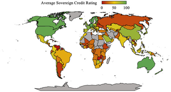
Figure 1.
Average sovereign credit ratings.
In Figure 1, green represents a higher rating, yellow represents a medium-level rating, and red represents non-investment grades.
Accordingly, Figure 2 illustrates the Biodiversity & Habitat Index by the Yale Center for Environmental Law and Policy (YCELP).
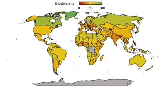
Figure 2.
Biodiversity Index.
Figure 2 shows the Biodiversity & Habitat Index by the Yale Center for Environmental Law and Policy (YCELP). Similar to Figure 1, higher scores are represented by green, while yellow represents medium scores. The lowest scores are represented by red.
Interpreting Figure 1 and Figure 2 presents diverging outcomes. While it is expected that a higher credit rating accompanies a higher level of biodiversity, it is not always the case. For instance, a country with a high credit rating does not always have a high biodiversity level, such as the cases of the USA and Australia. These countries have a medium level of biodiversity. Similarly, countries with low credit ratings such as Russia and Venezuela may be represented by high biodiversity. Thus, the research question of this study is whether consider biodiversity is a direct indicator of credit ratings. Accordingly, in our hypothesis, even if the results seem to be contradicting, biodiversity is considered to affect credit ratings adversely in accordance with the recent literature.
The aim of this study is to reveal the relationship between sovereign credit ratings and biodiversity since biodiversity is considered an important ESG credit factor. Following the recent literature, the article focuses on the impact of biodiversity on sovereign credit ratings as an accurate determinant. This study consists of six sections structured as follows: the second part presents a summary of the literature review; the third section briefly describes the data and methodology; the fourth section provides the empirical results and discussion; the fifth part of the study displays a robustness check of analyses; and lastly, the sixth section reports the conclusions and policy recommendations.
2. Literature Review
Sovereign economic assessments of the big three credit rating agencies show similarity in their frameworks according to the methodologies they use. This similarity can also be seen in the indicators chosen, such as GDP, GDP per capita, inflation, government debt, government expenditure, gross capital formation, savings, and trade openness [1,2,3]. This pattern can also be seen in the literature since these indicators are suggested to represent ratings significantly [4]. In the meantime, environmental awareness and sustainability approaches have induced new implementations, thus resulting in a shift in the literature accordingly. The shift can also be seen in rating agencies since environmental considerations were mentioned first and later included with subdimensions [1,3,8]. Hence, the literature review first focuses on the determinants of sovereign credit ratings to constitute a theoretical framework. The second part of the literature discusses the relationship between the determinants of ratings and the environment. The last part of the literature review investigates the relationship between the abovementioned variables and biodiversity.
2.1. Traditional Determinants of Sovereign Credit Ratings
Evaluating a country’s creditworthiness has been a challenging subject since determining valid economic indicators includes its own difficulties. In this manner, the research by Cantor and Packer [4] (p. 40) is substantial. The study’s approach is to use a more direct assessment technique than the rating agencies by considering only economic factors such as per capita income, GDP growth, inflation, fiscal balance, external budget, external debt, and dummy variables besides ratings. Similarly, Afonso [5] (p. 61) used per capita GDP, inflation, GDP growth, debt to exports ratio, and budget balance into account, in addition to development levels and default histories of countries. Further research by Afonso et al. [17] (p. 6) provided a similar estimation technique. The research considers GDP per capita, GDP growth, inflation, government debt, government balance, external debt, and current account similar to Cantor and Packer [4], but also suggests unemployment and reserves as indicators of sovereign credit ratings.
Mellios and Paget-Blanc [6] (p. 373) also examined the determinants of credit ratings. Their study used indicators of economy, money and banking, government finance, exchange rate, trade openness, external assets and liabilities, income, demographics, and society. Bissoondoyal-Bheenick [7] (p. 255) also measured the credit ratings by GNP per capita, inflation, financial balance, government debt, real exchange rate, foreign reserve, exports, unemployment, unit labor cost, current account, and foreign debt. Nonetheless, the models used in both analyses resemble the studies by Cantor and Packer [4] and Afonso [5].
Variables such as GDP growth, GDP per capita, inflation, fiscal balance, reserves, export, savings, gross domestic capital formation, and current account were also used in the process of investigating the sovereign credit ratings by Altenkirch [18] (p. 466). Another research study by Takawira and Mwamba [19] (p. 283) considered exchange rates, interest rates, debt-to-income ratio, unemployment, GDP growth, inflation, foreign debt, BoP, and current account balance as variables of credit ratings. Hereby, the literature may challenge the methodologies of rating agencies, and the use of similar determinants can also be seen. In this manner, these variables should be examined not only for their significance levels but also for how established they are.
2.2. Integration of ESG Indicators into Credit Ratings
While economic variables help in foreseeing and determining sovereign credit ratings, they do not take environmental awareness into account. Pineau et al. [20] (p. 3) used data similar to those in the aforementioned literature, in addition to environmental variables. CO2 emissions, agricultural land, food production index, agriculture, forest area, and depletion in natural resources were chosen to represent environmental effects. Another study by Klusak et al. [21] (p. 5954) investigated the relationship between sovereign credit risk (CDS) and the environment. Although the analysis used credit default swaps instead of credit ratings, the variables they used showed similarities. The environmental protection index by Yale University was also included in the analyses, which includes the effects of air quality, health, water, biodiversity, climate and energy, water, forests, fisheries, and agriculture. The study investigated the impact of the environment as a whole on sovereign risks by using CDS.
Research on credit ratings and the environment vary. For instance, Sun et al. [22] analyzed the relationship between credit ratings and the climate. This study used variables similar to Cantor and Packer [4] and Afonso [5] by exploring how ratings are related to climate risk. The results indicated that climate risk impacts credit ratings negatively. Anand et al. [23] conducted similar research on ESG factors and sovereign credit risk, although their study used CDS spread over credit ratings to determine sovereign credibility. Nevertheless, their study suggested that ESG factors are significant in credit ratings. Moreover, Hill Clarvis et al. [24] tried to establish a relationship between sovereign credit ratings and the environment, which was found to be significant in both the long term and the short term.
The importance of environmental factors on the economy can be seen in further research such as Dasgupta et al. [25] and Han and Cheng [26]. These studies revealed the significance of the environment on common goals. Dasgupta et al. [25] discussed the importance of the sustainable development goals of the United Nations within the scope of the ecological footprint. Their study revealed how sustainability is important for maintaining the global GDP per capita, which is a determinant in credit rating methodologies. Moreover, Han and Cheng [26] analyzed the effects of Paris Agreement Commitments on financial management and suggested a significant relationship between financial stability and the environment. Additionally, Byrne and Vitenu-Sackey [27] argued that climate risk is related to the macroeconomy by indicating that global risks are more substantial than country-specific ones. Lastly, Witajewski-Baltvilks and Fischer [28] focused on the spillover effect of using environmentally friendly technologies, while Eskander and Fankhauser [29] investigated the link between CO2 emissions and climate regulations. Contradicting expectations, the findings of the latter suggested no direct legislative impact. These studies may not be directly related to credit ratings, but they imply macroeconomic results. Overall, the relationship between ESG factors and credit ratings has been a popular subject in the literature.
2.3. Role of Biodiversity in Economic and Financial Modeling
ESG factors may be well integrated into the credit ratings, but recent literature has shown a shift toward environmental implications on sovereign credit ratings. Since credit rating agencies also mention environmental factors as indicators, research on the relationship between environmental variables and sovereign credit ratings is also significant. One notable variable that can be considered is biodiversity, with many related studies. For instance, Agarwala et al. [30] (p. 7) discussed why biodiversity plays a noticeable role in investment decisions. The consideration of biodiversity in credit ratings is credited to the economic implications of nature and the inability to identify all the risks that can result in losses. Similarly, Barbier [31] (p. 68) implied how global trade can be affected by biodiversity loss with respect to international agreements. The study suggests a worldwide increase in biodiversity, which is beneficial to all income levels. Accordingly, Chaudhary and Brooks [32] (p. 184) stated that biodiversity is linked to global trade and that the impacts of biodiversity are also carried with it. Another research study by Lenzen et al. [33] tackled the issue in developing nations by emphasizing the importance of research on biodiversity rather than remote pollution causes.
Studies related to biodiversity and international trade can be expanded. Li et al. [34], Morton et al. [35], Ortiz et al. [36], and Youm et al. [37] implemented comparable issues in their investigations. While Li et al. [34] (p. 5) approached the issue using the Red List of Threatened Species database as an indicator of biodiversity, Morton et al. [35] analyzed how wildlife trade influences biodiversity. The studies by Ortiz et al. [36] and Youm et al. [37] correlate with Li et al. [34] and Morton et al. [35] by interpreting the relationship between biodiversity and international trade. Consequently, the recent literature is paving the way for further research.
Biodiversity can also be linked to financial issues. Hutchinson and Lucey [38] present an integrative approach to the literature by stating the importance of biodiversity challenges. Anyango-van Zwieten [39] (p. 30) also addressed the issue by expressing the importance of allocating financial funds, while Arlaud et al. [40] (p. 88) stated that investments in biodiversity can strengthen financial outcomes. Karolyi and Tobin-de la Puente [41] (pp. 231–249) provided further insights into the significance of biodiversity loss and the accompanying risks involved with it. Hence, these studies suggest an in-depth analysis of the issue.
Further research on biodiversity and finance has been augmented in recent years. For instance, Oktaviani et al. [42] investigated how biodiversity can be enriched through various financial solutions. In addition, Githiru et al. [43] drew attention to the lack of funds for protecting biodiversity, while Nedopil et al. [44] emphasized the importance of potential risks to biodiversity related to the destructive results of financial applications. Similar research can be seen in the studies by Seidl et al. [45], Seidl et al. [46], and Wilson [47] where biodiversity investments, biodiversity credits, and sustainable finance applications were the main focus, respectively. Furthermore, Nedopil [48] drew attention to the impact of biodiversity on financial decision-making processes, whereas Phelps et al. [49] indicated the importance of balancing conservation and financial risks. Since the risks involved can be measured by a country’s creditworthiness, Semet, et al. [50] revealed how governance and social indicators are related to credit ratings, but environmental variables are not truly represented by credit rating agencies.
Evaluating a country’s creditworthiness has been a challenging subject since determining valid economic indicators includes its own difficulties. In this manner, the research by Cantor and Packer [4] (p. 40) is substantial. Their approach was to use a more direct assessment technique than the rating agencies by considering only economic factors such as per capita income, GDP growth, inflation, fiscal balance, external budget, external debt, and dummy variables, in addition to ratings. Similarly, Afonso [5] (p. 61) took per capita GDP, inflation, GDP growth, debt-to-exports ratio, and budget balance into account, in addition to the development levels and default histories of countries. Another research study by Afonso et al. [17] (p. 6) provided a similar estimation technique. Their research considered GDP per capita, GDP growth, inflation, government debt, government balance, external debt, and current accounts, similar to Cantor and Packer [4], but also suggested unemployment and reserves as indicators of sovereign credit ratings.
The literature on the subject reveals the importance of a detailed analysis of credit ratings. Rather than focusing on economic factors only, ESG factors should also be included in the analysis. A more in-depth analysis can fill the gap in the literature by using subdimensions. Thus, this study focuses on the relationship between sovereign credit ratings and biodiversity.
3. Materials and Methods
3.1. Data Specification
The literature reveals that structural changes, such as gross domestic product, per capita income, consumer price index, gross debt stocks, final consumption expenditure, capital formation, savings, and trade openness, affect sovereign credit ratings [4]. Therefore, this paper examines whether biodiversity impacts sovereign credit ratings more severely as it is regarded as the main determinant of countries’ economic development and sustainability. The biodiversity index evaluates national efforts to conserve natural ecosystems and the full spectrum of biological diversity within a country’s territory. It is composed of twelve distinct indicators: the protection of marine biodiversity, the safeguarding of key marine and coastal habitats, marine conservation initiatives, the protected areas representativeness index, the Species Habitat Index, the Species Protection Index, the conservation of terrestrial biomes, terrestrial biodiversity preservation, management effectiveness of protected areas, the extent of agricultural activities within conservation zones, the Red List Index, and the bioclimatic ecosystem resilience index. Notably, the Red List Index functions as a subcomponent of the broader biodiversity index, estimating species’ extinction risk by assigning weights based on the proportion of their range that falls within a specific national or regional boundary. These two environmental sustainability metrics were chosen due to their integrative scope, encompassing various other ecological indicators such as forest cover and species richness. Accordingly, following the recent literature, this article focuses on the impact of biodiversity on sovereign credit ratings as an accurate determinant of sovereign credit ratings [30]. While the prominence of Environmental, Social, and Governance (ESG) factors for countries has surged in recent years, issues concerning environmental protection have been a subject of debate since the early 2000s [51]. Accordingly, this study utilized annual datasets sourced from ten distinct sources spanning from 2001 to 2021 for the variables under investigation. The dataset contains the variables of sovereign credit ratings, gross domestic product, per capita income, consumer price index, gross debt stocks, final consumption expenditure, capital formation, savings, trade openness, biodiversity index, and the Red List Index. Data for S&P, MOODY’S, and FITCH credit ratings were sourced from the Trading Economics and Country economy databases. Macroeconomic indicators—including gross domestic product, consumer price index, general government final consumption, gross capital formation, gross savings, and trade openness—were extracted from the World Bank database. Additionally, information on general government gross debt was obtained from the International Monetary Fund (IMF). Biodiversity-related indicators were retrieved from the Yale Center for Environmental Law and Policy (YCELP), while data on the Red List Index were accessed through the Organisation for Economic Co-operation and Development (OECD) database. Table 1 provides the descriptions, measurement units, and data sources for the variables used in the econometric models.

Table 1.
Definitions and sources of variables.
This study examines a global sample of 62 countries, accounting for 91% of the world’s GDP and 81% of the world’s greenhouse gas emissions, to derive policy implications related to biodiversity. The selection of these countries was based on their environmental quality and pollution levels, encompassing a mix of developing, developed, and least-developed economies. Furthermore, these 62 nations represent a significant portion of the global economy, collectively producing 91% of the world’s gross domestic product and 81% of the world’s greenhouse gas emissions.
In the literature, sovereign credit ratings are often indexed by a 20-point or a 60-point scale. Those who only consider investment grades use the first method. A more in-depth analysis to include the ratings’ outlook can be conducted by the second method, but it lacks representing ratings’ watches. This study differs from the general literature by using a 100-point scale to address sovereign credit ratings given by S&P Global, Moody’s, and Fitch. Even though there are 20 levels for each investment grade, outlooks and watches are also included for better estimations. Positive, stable, or negative outlooks are given by the agencies when the determinants are explanatory in the ratings; in other words, when the economic situation is from a known source. When the economic situations are from an unknown source, the ratings include positive or negative watches. Therefore, 20 levels of grades are combined with 5 levels of outlooks and watches, represented by a 100-point scale. The sovereign credit rating index is given in Table A3.
3.2. Empirical Model
This paper focuses on biodiversity as a determinant of sovereign credit ratings. Similar to Cantor and Packer [4], the control variables are GDP, GDP per capita, consumer price index, general government gross debt, general government final consumption expenditure, gross capital formation, gross savings, and trade openness. GDP represents the size of countries’ economies. GDP per capita (GDPpc) reflects the influence of economic growth and income levels on sovereign credit ratings. CPI tracks the temporal variation in the overall price levels of goods and services commonly purchased for consumption. DEBT refers to the total debt that all institutions and organizations under the direct or indirect control of the state are obliged to pay to the world outside the public sector as of a certain period. Purchasing goods and services by governments to directly meet the individual or social needs of society is measured by general government final consumption expenditure. CAPITAL shows the investments made in the country during a certain period. SAVINGS determines the economy’s capacity to create new capital. OPENNESS demonstrates how liberal or strict the policies are that countries apply in their commercial relations with the outside world. The research variable BIODIVERSITY is selected according to the research of Agarwala et al. [30], which suggests adjusting creditworthiness according to biodiversity changes.
Leveraging these variables, we develop an econometric framework grounded in Equations (1)–(3) to evaluate the influence of biodiversity on sovereign credit ratings, as detailed below:
In this context, i and t denote country and time, respectively. The stochastic component is represented by ε, while the coefficients , , , , , , , , and capture the long-term elasticities of the variables in the equations. Furthermore, the models utilized for robustness analysis are outlined below in Equations (4)–(6).
In accordance with the research model hypothesis, biodiversity is anticipated to adversely influence credit ratings, with its effects potentially shifting in either direction as national credit evaluations evolve [1,2,3]. Nevertheless, the association between biodiversity and credit ratings is projected to manifest both positive and negative dimensions, attributable to the varied methodological approaches employed by different credit rating agencies.
3.3. Dynamic Panel GMM Approach
Cyclical fluctuations, natural disasters, economic crises, and conflicts that occur in the global system affect the economic outlook of countries directly. Since the OLS estimator makes estimations based on the averages of the variables, its use for heterogeneous data may mislead the estimation results. Therefore, the paper employs a panel two-step system GMM approach developed by Arellano and Bover [52], and panel quantile regression models for heterogeneous data were implemented to analyze the linear effect of the GDP, GDP per capita, consumer price index, general government gross debt, general government final consumption expenditure, gross capital formation, gross savings, trade openness, biodiversity, and Red List Index on sovereign credit ratings in 62 countries that constitute 91% of the world’s GDP and 81% of the world’s greenhouse gas emissions as a global sample.
Given that the dataset in this study contains more cross-sectional observations (N) than time series observations (t), the most suitable method to apply is the Generalized Method of Moments (GMM) [53]. The dynamic panel GMM approach is selected because it addresses issues of endogeneity, autocorrelation, and heteroscedasticity effectively [54] The GMM approach was revealed in the studies of Anderson and Hsiao [55], Arellano and Bond [56], Arellano and Bover [52], and Blundell and Bond [57]. Anderson and Hsiao [55] and Arellano and Bond [56] produced the GMM first-differences estimator, which applies a differencing approach to fix endogeneity. The GMM first-differences estimator has a limitation due to the removal of previous data points from the current ones, which can exacerbate gaps in unbalanced datasets. In contrast, the System GMM estimator proposed by Blundell and Bond [57] and Arellano and Bover [52] addresses this issue by using orthogonal deviations, which eliminates the average of the variable’s future observations, providing a more balanced approach. Considering this information, the System GMM estimator is used in this paper. The System GMM estimator put forward by Arellano and Bover [52] and Blundell and Bond [57] is based on the following regression model (7)–(12):
where β represents the coefficients, X represents the control variables (GDP, GDPpc, CPI, DEBT, EXPEND, CAPITAL, SAVING, and OPENNESS), τ represents a lag order, and ε represents the two-way disturbance term.
3.4. Panel Quantile Regression
Various econometric techniques are common for examining panel data. Most of the existing papers have used traditional methods to discover the factors affecting sovereign credit ratings, but these approaches have conditional expectations regarding the dependent variable and fail to reveal the correct results [58]. Binder and Coad [59] argued that conventional regression methods might produce inaccurate estimates of significant coefficients or fail to identify key relationships, as they primarily emphasize mean effects. Moreover, the relationships among the variables are difficult to determine distinctly at different quantiles (i.e., to perform differently across countries with different levels of sovereign credit ratings) due to the enormous heterogeneity in the global panel. Alternatively, the influence of biodiversity and related variables is likely to differ across nations depending on their sovereign credit rating. Therefore, in this paper, the panel quantile regression model proposed by Koenker and Bassett [60] is employed to examine the effects of gross domestic product, per capita income, consumer price index, gross debt stocks, final consumption expenditure, capital formation, savings, trade openness, and biodiversity on sovereign credit ratings in the global panel. The econometric model is presented as follows to perform the quantile function of the panel data (13):
where is the quantile of the dependent variable, is the vector of the independent variables, is the quantile, and is the regression parameter of the th quantile. The panel quantile estimates in this paper can be specified as (14)–(16):
where , , and are the conditional quantile (th) of the dependent variable, while denotes the vector of explanatory variables for country i in year t at quantile τ. The coefficient β corresponds to the slopes of the explanatory variables for the specified quantile τ.
4. Empirical Results and Discussion
4.1. Preliminary Analysis
Table 2 presents the descriptive statistics for the variables used in the research model. These statistics are analyzed to assess the normality of the data. The summary results confirm that the data are normally distributed and free of outliers. Consistent with these findings, none of the variables show deviations from a normal distribution. The appropriate estimator is crucial for evaluating both the cross-sectional dependence and slope homogeneity in panel data analysis. Given the increasing interconnectedness of countries within highly globalized economies, considering cross-sectional dependence and heterogeneity is essential in the analyses of panel data studies. These analyses investigate the presence of cross-sectional dependence and heterogeneity among the countries represented in the model. To evaluate cross-sectional dependence, the Breusch–Pagan LM test [61], the Pesaran scaled LM test [62], and the Pesaran CD test [62] are employed. The findings presented in Table A1 reveal a statistically significant rejection of the null hypothesis, indicating the existence of cross-sectional dependence among the countries. In other words, the p-value for all models was statistically significant at the 1% level (p < 0.01). This suggests that economic shocks in any of the 62 nations, collectively representing 91% of the global GDP and 81% of the world’s greenhouse gas emissions, have implications for others. Furthermore, the outcomes of slope homogeneity tests, as proposed by Swamy [63] and Pesaran and Yamagata [64], are also detailed in Table A1. These results highlight the inclusion of country-specific effects within the models.
Table 2.
Preliminary statistics.
Table A2 presents the results of the first-generation unit root tests conducted by Im et al. [65] and Breitung [66]. These tests, however, do not account for cross-sectional dependence in the data. To address this limitation, the second-generation unit root test proposed by Pesaran [67] is also applied, with the corresponding results included in Table A2. These tests evaluate the stationarity of the series. The findings indicate that while the variables exhibit a unit root at their levels [I(0)], they become stationary after taking the first differences [I(1)], particularly under the second-generation tests that incorporate cross-sectional dependence.
4.2. Empirical Results
Various studies have applied different estimators to examine the relationships between sovereign credit ratings and macroeconomic variables by using different objectives and data types. For instance, while Cantor and Packer [4] made use of multiple regression analysis, Kaminsky and Schmukler [68] and Kräussl [69] benefited from panel regressions in addition to case studies. DOLS was used by Badr and Elkhadrawi [70] and OLS dynamic panel data were used by Montes and de Oliveira [71]. In this study, an effective estimation method is necessary to accomplish our objective. In order to estimate the dynamic panel model, Generalized Method of Moments (GMM) estimators developed by Arellano and Bover [52] and Blundell and Bond [57] are employed. Specifically, the system GMM estimator introduced by Blundell and Bond [57] is used, as it is considered more efficient for panel data involving a large number of cross-sectional units (62 countries) over a relatively short time span (21 years) [72] (p. 7).
After the preliminary analyses, the panel GMM estimation of econometric models is performed. The explained panel GMM model results in this paper are shown as the findings from the System GMM model. According to the diagnostic tests, the results state that there is no first-order autocorrelation (AR1) and second-order autocorrelation (AR2) [56]. The Hansen J-test for instrument validity provided strong statistical evidence supporting the validity and robustness of the instruments used (p > 0.05). This outcome is reflected in the inability to reject the over-identifying restrictions. We apply the system GMM model in this paper to address the limitations of other estimation models.
The findings of the GMM estimation in Table 3 demonstrate significant positive effects of the first lag of S&P, FITCH, and MOODYS on the current S&P, FITCH, and MOODYS in the panel. The Systems GMM model results indicate that an increase in the first lags of S&P, FITCH, and MOODYS by 1% causes an increment in the current S&P, FITCH, and MOODYS by 0.56%, 0.8%, and 0.78%, respectively. In this regard, past positive values of S&P, FITCH, and MOODYS increase S&P, FITCH, and MOODYS in the future. The findings also present that GDP is negatively linked to sovereign credit ratings in these countries. An increase in GDP by 1% causes S&P, FITCH, and MOODYS to decrease by 0.7%, 0.59%, and 0.64%, respectively. The results also suggest that S&P improves with an increment in GDP per capita. In particular, a 1% increase in GDPpc ensures a 0.2% increment in the S&P. However, the consumer price index in these countries is observed to have a significant negative effect on sovereign credit ratings. An increase in CPI by a unit causes S&P, FITCH, and MOODYS to decrease by 0.07%, 0.05%, and 0.06%, respectively. Likewise, the relationship between government gross debt and sovereign credit ratings shows that a unit increase in DEBT will lead to a decline of 0.15%, 0.06%, and 0.06% in S&P, FITCH, and MOODYS, respectively. Moreover, government final consumption expenditure is observed to have a positive effect on sovereign credit ratings. In this regard, a rise in EXPEND by 1% causes S&P, FITCH, and MOODYS to increase by 0.41%, 0.18%, and 0.3%, respectively. In addition, a significant positive effect on sovereign credit ratings by gross capital formation is determined. An increment in CAPITAL in these countries by 1% causes S&P, FITCH, and MOODYS to rise by 0.25%, 0.28%, and 0.27%, respectively. Furthermore, gross savings and trade openness are confirmed to ensure a significant positive effect on sovereign credit ratings. An increase in SAVING in these countries by a unit causes S&P, FITCH, and MOODYS to increase by 0.11%, 0.11%, and 0.1%, respectively, while a rise in OPENNESS by a unit causes S&P, FITCH, and MOODYS to increase 0.32%, 0.36%, and 0.24%, respectively. The paper aims to reveal the effects of biodiversity on sovereign credit ratings. As a result of the GMM estimation, biodiversity’s negative effect on credit scores is determined. In this direction, a unit increase in BIODIVERSITY causes a decrease in S&P, FITCH, and MOODYS by 0.23%, 0.07%, and 0.05%, respectively.
Table 3.
Panel GMM estimation results.
Table 4 presents the outcomes of the panel quantile regression analysis, examining the impact of macroeconomic variables and biodiversity on sovereign credit ratings across a global panel of 62 countries. The results are shown for various percentiles of the distribution (5th, 10th, 20th, 90th, and 95th) of each dependent variable. According to the results in Table 4 with the panel quantile regression model, GDP, CPI, and DEBT significantly and negatively affect sovereign credit ratings across all quantiles, while GDPpc, EXPEND, CAPITAL, SAVING, and OPENNESS significantly and positively impact sovereign credit ratings across all quantiles. On the other hand, BIODIVERSITY has both significant positive and negative impacts on sovereign credit ratings in different quantiles, similar to revelations made by Bartelmus [73] and Christie et al. [74]. BIODIVERSITY significantly and positively affects S&P, FITCH, and MOODYS until the 40th, 50th, and 50th quantiles, respectively, whereas it significantly and negatively impacts S&P and MOODYS in the 60th–70th and 70th–90th quantiles, respectively. In addition, BIODIVERSITY has significant positive effects on S&P in the 90th–95th quantiles. These empirical findings are in line with many established studies such as Cantor and Packer [4] and Afonso et al. [17] regarding long-term sovereign credit ratings. The results are also valuable considering the suggestions made by Nedopil [44] and Phelps et al. [49] on biodiversity and financial risks. The introduction of BIODIVERSITY as a determinant of sovereign credit ratings fills the gap in the literature suggested by Semet et al. [50].
Table 4.
Panel quantile regression results.
A summary of the coefficient signs of the panel quantile regression is demonstrated in Table 5. Overall, this paper reveals that GDP is negative at low, middle, and high quantiles, while GDPpc is positive in all quantiles. In addition, CPI and DEBT are negative in all quantiles, whereas EXPEND, CAPITAL, SAVING, and OPENNESS are positive at low, middle, and high quantiles. Moreover, BIODIVERSITY is positive in the lower quantiles while being both negative and positive in the middle and high quantiles. These findings suggest that as nations become more economically advanced, they tend to achieve higher credit scores, likely because environmental considerations are often sidelined amid intense industrial production and commercial activity. Economies heavily dependent on natural resources often exhibit limited structural transformation, alongside patterns of unsustainable and inequitable growth. Following the recent commodity boom, the critical challenge for both developed and developing nations has been how to leverage resource-based revenues to foster economic expansion, diversification, and inclusive, sustainable development—without compromising biodiversity. In this regard, resource-rich countries have increasingly encountered what is referred to as the “resource curse”, whereby rapid industrialization and reliance on extractive sectors transform natural wealth into an economic liability [75]. This dynamic has been particularly evident in nations striving for elevated growth rates and favorable credit ratings. As such, industrializing economies with strong credit profiles must prioritize harmonizing biodiversity conservation with their development agendas to ensure long-term ecological and economic resilience.
Table 5.
Summary of quantile regression results.
The finding that biodiversity has a negative relationship with sovereign credit ratings in higher quantiles runs counter to expectations and suggests the need to investigate underlying institutional and economic factors in highly rated countries. These countries typically have well-developed service and industrial sectors, where biodiversity-dependent industries—such as agriculture, forestry, or tourism—contribute minimally to the overall output. As a result, biodiversity is often underrepresented in fiscal assessments. Additionally, advanced economies may prioritize infrastructure growth and resource-intensive development, leading to greater biodiversity loss. Ironically, their strong institutions and fiscal tools can support activities that degrade ecosystems for short-term economic gain. This suggests a systemic undervaluation of ecological assets, pointing to a disconnect between biodiversity’s real importance and how it is reflected in financial evaluation frameworks.
5. Robustness Check
The robustness of our findings is verified using panel GMM estimation and the panel quantile regression approach, as shown in Table 6 and Table 7, with the inclusion of our robustness variable. For the 62 countries that constitute 91% of the world’s GDP and 81% of the world’s greenhouse gas emissions, our results reveal that GDPpc, EXPEND, CAPITAL, SAVING, and OPENNESS significantly and positively impact sovereign credit ratings. On the other hand, GDP, CPI, DEBT, and REDLIST decrease the sovereign credit ratings of the 62 countries that constitute 91% of the world’s GDP and 81% of the world’s greenhouse gas emissions. The biodiversity variables in this paper, which are primary and robust research variables such as BIODIVERSITY and REDLIST, decrease sovereign credit ratings.
Table 6.
Robustness check of panel GMM estimation results.
Table 7.
Robustness check of panel quantile regression results.
The robustness check results of the panel GMM estimation show that increases in economic welfare, government final consumption expenditure, gross capital formation, gross savings, and trade openness affect sovereign credit ratings positively for the 62 countries constituting 91% of the world’s GDP and 81% of the world’s greenhouse gas emissions. In contrast, an increase in economic growth, inflation, and government gross debt reduces the sovereign credit ratings according to the robustness check results. Moreover, the Red List Index in these countries negatively affects sovereign credit ratings in line with panel GMM test results.
Table 7 presents the robustness results from panel quantile regression analyses, where REDLIST is used as the research variable. According to the robustness test results, GDP, CPI, and DEBT have negative and statistically significant effects on credit ratings across all quantiles, while GDPpc, EXPEND, CAPITAL, SAVING, and OPENNESS show statistically significant and positive effects in the 62 countries that constitute 91% of the world’s GDP and 81% of the world’s greenhouse gas emissions. According to the robustness analysis, REDLIST has statistically significant and positive effects on S&P between the 50th and 80th quantiles and yet exhibits a negative and significant effect at the 95th quantile. Furthermore, REDLIST positively and significantly influences FITCH between the 30th and 60th quantiles but has a negative and significant impact at the 95th quantile. Additionally, REDLIST has a statistically significant and positive impact on MOODYS between the 20th and 50th quantiles, while a negative and significant effect is observed at the 80th quantile. The robustness check findings are consistent with prior analyses, suggesting that when the emphasis on environmental and biodiversity factors increases, sovereign credit ratings tend to improve in countries with low to medium grades. Conversely, in countries with high grades, increased emphasis on environmental and biodiversity factors correlates with a decrease in sovereign credit ratings.
Despite the robustness of the empirical strategy and the use of comprehensive cross-country data, this study is subject to several limitations that should be acknowledged. First, the analysis relies on proxy indicators to quantify biodiversity and related ecological variables. While indices such as the Red List Index and the Species Habitat Index are widely recognized, they may not fully capture the multidimensional nature of biodiversity or localized ecological nuances. Second, potential measurement errors in both biodiversity metrics and macroeconomic variables may introduce bias, particularly in countries with limited data availability or inconsistent reporting standards. Third, although the use of the panel Generalized Method of Moments (GMM) estimator helps address endogeneity concerns, such as reverse causality and omitted variable bias, endogeneity cannot be entirely ruled out due to the complex interactions between environmental conditions and sovereign credit dynamics. Lastly, while this study identifies statistically significant relationships, care must be taken in interpreting the practical relevance of these effects, particularly when considering heterogeneity across countries and over time. Future research could benefit from higher-resolution data, dynamic ecological modeling, and case-specific analyses to complement and deepen the insights presented here.
6. Conclusions and Policy Recommendation
As international competitiveness intensifies, countries have increasingly focused on enhancing their sovereign credit ratings through high levels of economic growth and industrialization. However, rapid industrialization has significant impacts on ecological balance. This article analyzes the effects of macroeconomic variables and biodiversity on sovereign credit ratings over the period of 2001 to 2021. To achieve this, we employ panel GMM and panel quantile regression analyses on data from the 62 countries that constitute 91% of the world’s GDP and 81% of the world’s greenhouse gas emissions.
The results of the panel GMM analyses indicate that countries’ per capita income, expenditures, capital accumulation, savings, and trade openness positively influence credit ratings, similar to the findings of Cantor and Packer [4]. However, economic growth impacts credit ratings negatively, in line with the research of Block and Vaaler [76] and Montes and de Oliveira [71]. Inflation and debt levels are also found to negatively affect credit ratings, resembling research by Badr and Elkhadrawi [70]. Additionally, an increase in countries’ biodiversity levels has a negative impact on credit ratings. The empirical findings for the Red List Index, considered an additional indicator of biodiversity, are consistent with the results for the biodiversity index in the baseline research model. Developing approaches that account for environmental impacts alongside economic development is expected to yield results in line with expectations, where both biodiversity and the Red List Index negatively influence credit ratings for the 62 countries that constitute 91% of the world’s GDP and 81% of the world’s greenhouse gas emissions.
The panel quantile regression results in our study reveal that per capita income, expenditures, capital accumulation, savings, and trade openness have a positive impact on sovereign credit ratings across all quantiles. Conversely, economic growth, inflation, and debt levels negatively affect sovereign credit ratings across all quantiles. Additionally, biodiversity has a negative effect on sovereign credit ratings at medium and high quantiles. The robustness analyses indicate that the Red List Index also has a negative impact on sovereign credit ratings at higher quantiles. The findings from the panel quantile regression suggest that efforts to improve ratings in an environmentally sensitive manner by countries with high sovereign credit ratings may lead to negative impacts on those ratings. Thus, it is crucial to consider environmental factors, such as biodiversity, in sovereign credit rating assessments. The results can be considered valuable since the findings are in line with the studies focusing on environmental impacts such as Dasgupta et al. [25] and Byrne and Vitenu-Sackey [27]. The findings also confirm the suggestions of Agarwala et al. (2022) [30] and Barbier [31] on biodiversity and nature loss. Finally, Hutchinson and Lucey [38], Arlaud et al. [40], and Oktaviani et al. [42] have all stated the impact of biodiversity on financial issues, which increases the value added to the literature with the results of this study.
The findings from the analyses in this article provide the first evidence of the impact of biodiversity and the Red List Index on sovereign credit ratings across these 62 countries that constitute 91% of the world’s GDP and 81% of the world’s greenhouse gas emissions. In other words, our paper demonstrates how environmental factors, such as biodiversity, can have a significant impact on sovereign credit ratings alongside other macroeconomic variables. Additionally, our paper supports previous studies in the literature that examine the effects of economic growth, per capita income, inflation, debt levels, expenditures, capital accumulation, savings, and trade openness on sovereign credit ratings [17,18]. Furthermore, empirical results indicate that environmental factors have significant effects on sovereign credit ratings, corroborating prior findings [30].
The results of the econometric forecasts present the expected signs of the determinants of sovereign credit ratings found in the literature. In addition, the findings from the panel quantile regression analysis reveal that the effects of environmental factors on sovereign credit ratings vary according to the credit rating levels of countries. This paper suggests that as countries’ sovereign credit ratings increase, the influence of environmental factors shifts in a negative direction. Therefore, this paper contributes to the discussion on the relationship between sovereign credit ratings and environmental factors conducted by Sun et al. [22], Anand et al. [23], and Hill Clarvis et al. [24].
This paper identifies the main determinants of credit ratings for the 62 countries that constitute 91% of the world’s GDP and 81% of the world’s greenhouse gas emissions. Investment-grade countries, which have higher credit ratings, would receive lower ratings if environmental factors were taken into account. In contrast, speculative-grade countries, with lower credit ratings, could achieve higher ratings by considering environmental factors. Furthermore, higher economic growth and credit ratings are indicative of environmental issues. In this regard, international public opinion and organizations can exert pressure on these countries and credit agencies to consider environmental factors, potentially limiting environmental degradation and ensuring more realistic credit ratings.
The analysis reveals that nations with low credit ratings are more likely to secure increased multilateral support or environmental grants, which can enhance their environmental protection budgets and ultimately bolster biodiversity. Consequently, rather than attaining elevated credit ratings as a byproduct of improved biodiversity, countries with lower ratings might leverage international assistance to achieve biodiversity gains. Nonetheless, the occurrence of warfare or natural disasters can simultaneously degrade environmental conditions, thereby reducing biodiversity and undermining financial stability, which in turn may lead to diminished credit ratings. These concurrent shocks could establish a positive correlation through both direct and indirect channels. Moreover, developed countries with high credit ratings might continue extracting natural resources intensively or rapidly industrializing, inadvertently harming biodiversity. In such cases, abundant capital from high credit ratings coupled with intensified resource use can inflate production volumes, thereby complicating the straightforward relationship between biodiversity loss and declining credit ratings.
This paper also highlights, as pointed out by Pineau et al. [20] and Klusak et al. [21], that giving greater weight to environmental factors in the calculation of countries’ sovereign credit ratings could contribute to a more sustainable environment. However, this largely depends on the collective will of developed countries with higher sovereign credit ratings. In the coming years, increased discussions on reducing environmental degradation and the impact of environmental factors on countries’ sovereign credit ratings are expected. Therefore, updates should be made to the methods used in calculating sovereign credit ratings and the variables that influence these ratings. Biodiversity evaluation relies on integrated indices that reflect species richness, ecological variety, and genetic variation, often analyzed alongside spatial and temporal patterns. These assessments typically draw on three categories of indicators: species-level metrics, ecosystem-level indicators, and environmental pressure variables. Among species-level measures, key indices such as the Red List Index (RLI), Species Habitat Index (SHI), and Species Protection Index (SPI) are relevant for informing sovereign credit assessments. The RLI monitors changes in extinction risk across multiple taxa, the SHI quantifies habitat condition and spatial availability over time, and the SPI assesses the degree of species range coverage within protected areas. Complementing these, ecosystem-based indicators such as the protected areas representativeness index (PARI), terrestrial and marine biome representation (TMBR), and the bioclimatic ecosystem resilience index (BERI) offer further insight. PARI gauges how effectively protected areas capture a nation’s ecosystem diversity, TMBR evaluates biome-specific conservation performance, and BERI models an ecosystem’s potential to maintain biodiversity under future climate scenarios. Additionally, indicators of anthropogenic pressure—such as land conversion, the expansion of agricultural frontiers, pollution levels, and rates of natural resource exploitation—serve as critical contextual variables in biodiversity analysis and can meaningfully inform sovereign credit rating frameworks by highlighting underlying environmental risks. Biodiversity indicators can function as predictive markers of long-term economic resilience and sustainable development trajectories. Integrating ecological indicators into sovereign credit evaluations is both a responsible approach to environmental stewardship and a vital component in maintaining sustainable financial systems in the long term.
Policy differentiation based on sovereign credit ratings offers a strategic pathway for aligning biodiversity objectives with national economic conditions. Countries with high credit ratings typically benefit from robust institutions, stable fiscal environments, and mature regulatory systems. These attributes position them well to integrate biodiversity considerations into fiscal and financial policies. Strategies may include the issuance of green or biodiversity-linked bonds tied to verifiable conservation outcomes and the incorporation of biodiversity metrics into national budgeting frameworks. Furthermore, such countries can enhance their role in global environmental governance by expanding international biodiversity finance commitments, facilitating technology transfers, and supporting biodiversity initiatives in low-income regions through multilateral climate and conservation mechanisms. Strengthening private sector accountability is also critical in high-credit contexts. Mandating biodiversity-related disclosures within environmental, social, and governance (ESG) reporting standards can drive corporate responsibility and transparency in natural capital use. Conversely, countries with lower credit ratings—often constrained by limited fiscal capacity and greater reliance on natural resource extraction—require targeted, cost-effective policy frameworks. These should emphasize institutional strengthening, particularly through governance reforms that integrate biodiversity into spatial planning and development strategies. Promoting nature-based solutions that deliver multiple benefits—for climate adaptation, water security, and community livelihoods—can offer substantial returns at lower costs. Inclusive, participatory governance involving local and Indigenous communities is essential for ensuring the legitimacy, effectiveness, and long-term sustainability of biodiversity actions. In summary, tailoring biodiversity policy to a country’s credit profile allows for the reconciliation of ecological priorities with economic and institutional realities. A rigorous, evidence-based policy architecture ensures that both high- and low-rated nations can effectively contribute to global biodiversity targets while enhancing their resilience to environmental and economic shocks. Embedding biodiversity into sovereign financial systems is not only vital for ecological preservation but also fundamental to sustainable economic development.
Moreover, countries investing in sustainability will gain a comparative advantage in the global economy in the future. For instance, studies like Dasgupta et al. [25] draw attention to UN sustainable development goals, while Han and Cheng [26] pay attention to the effects of Paris Agreement Commitments on financial management. While countries may strive to maintain high sovereign credit ratings to achieve economic and commercial objectives, this focus could ultimately lead to the disruption of ecological balance through environmental degradation. Emphasizing the potential benefits of incorporating environmental considerations into sovereign credit rating evaluations—and conducting separate regression analyses for developed and developing nations—can offer critical insights for shaping future policy. This approach may contribute significantly to mitigating climate change and curbing environmental degradation, while also enhancing the understanding of how environmental risks influence macroeconomic and financial stability.
Author Contributions
Conceptualization, M.K.İ.; methodology, A.Ş.; software, A.Ş. and M.K.İ.; validation, A.Ş.; formal analysis, A.Ş. and M.K.İ.; investigation, A.Ş. and M.K.İ.; resources, M.K.İ.; data curation, A.Ş.; writing—original draft, A.Ş. and M.K.İ.; writing—review and editing, M.K.İ.; visualization, A.Ş. and M.K.İ.; supervision, A.Ş. and M.K.İ.; project administration, A.Ş. and M.K.İ. All authors have read and agreed to the published version of the manuscript.
Funding
This research received no external funding.
Institutional Review Board Statement
Not applicable.
Informed Consent Statement
Not applicable.
Data Availability Statement
The raw data supporting the conclusions of this article will be made available by the authors upon request.
Acknowledgments
The authors would like to thank the anonymous referees for their constructive comments.
Conflicts of Interest
The authors declare no conflicts of interest.
Appendix A
Table A1.
Cross-sectional dependence and homogeneity tests.
Table A1.
Cross-sectional dependence and homogeneity tests.
| Test | Equation (1) | Equation (2) | Equation (3) |
|---|---|---|---|
| CDBP | 9792.049 *** | 9896.843 *** | 9937.228 *** |
| CDLM | 128.477 *** | 130.181 *** | 130.837 *** |
| CD | 29.548 *** | 22.663 *** | 44.009 *** |
| 9.941 *** | 12.149 *** | 9.013 *** | |
| adj | 14.406 *** | 17.606 *** | 13.061 *** |
| Swamy’s Test | 52,203.52 *** | 62,457.51 *** | 45,377.62 *** |
Note: *** indicate significance at 1% level.
Table A2.
First- and second-generation unit root test results.
Table A2.
First- and second-generation unit root test results.
| Variables | First-Generation Unit Root Test | Second-Generation Unit Root Test | ||||
|---|---|---|---|---|---|---|
| Im, Pesaran, and Shin | Breitung | PESCADF | ||||
| Intercept | Intercept and Trend | Intercept | Intercept and Trend | Intercept | Intercept and Trend | |
| Level | ||||||
| S&P | −2.073 *** | −0.332 | 1.569 | 4.168 | −1.641 | −2.061 |
| MOODYS | −7.497 *** | −3.376 *** | 2.468 | 5.021 | −1.586 | −1.758 |
| FITCH | −3.816 *** | −0.024 | 1.8543 | 5.052 | −1.336 | −1.756 |
| GDP | −2.558 *** | 0.116 | 15.496 | 4.899 | −1.674 | −1.396 |
| GDPpc | −2.431 *** | −2.662 *** | 11.862 | 3.103 | −1.736 | −1.585 |
| CPI | 1.787 | 4.875 | 21.252 | 8.194 | −1.642 | −1.251 |
| DEBT | 1.505 | 2.061 | 3.528 | 4.149 | −1.569 | −1.557 |
| EXPEND | 6.594 | 1.825 | 19.091 | 7.283 | −1.637 | −1.859 |
| CAPITAL | −2.295 ** | −1.611 * | 4.421 | 1.168 | −1.635 | −1.553 |
| SAVINGS | −5.683 *** | −0.942 | 7.928 | 2.237 | −1.937 * | −2.302 |
| OPENNESS | −1.146 | −3.682 *** | 0.167 | −2.319 *** | −1.527 | −2.027 |
| BIODIVERSITY | −11.906 *** | −19.699 *** | 9.331 | 3.538 | −1.371 | −2.129 |
| REDLIST | 7.989 | −58.051 *** | 18.356 | 3.774 | −1.542 | −1.781 |
| First Difference | ||||||
| S&P | −15.328 *** | −13.709 *** | −9.717 *** | −10.339 *** | −2.361 *** | −2.731 *** |
| MOODYS | −20.528 *** | −16.106 *** | −6.387 *** | −6.451 *** | −2.149 *** | −2.574 *** |
| FITCH | −14.768 *** | −14.003 *** | −10.807 *** | −9.501 *** | −2.113 *** | −3.474 *** |
| GDP | −20.079 *** | −18.958 *** | −16.872 *** | −5.335 *** | −3.085 *** | −3.095 *** |
| GDPpc | −20.759 *** | −18.196 *** | −16.609 *** | −5.538 *** | −3.081 *** | −3.113 *** |
| CPI | −11.912 *** | −10.477 *** | −7.591 *** | −4.053 *** | −2.155 *** | −2.894 *** |
| DEBT | −15.017 *** | −12.555 *** | −12.806 *** | −5.679 *** | −3.264 *** | −3.325 *** |
| EXPEND | −13.641 *** | −11.844 *** | −11.468 *** | −6.671 *** | −2.253 *** | −3.593 *** |
| CAPITAL | −20.776 *** | −17.285 *** | −15.814 *** | −9.866 *** | −2.515 *** | −2.987 *** |
| SAVINGS | −17.984 *** | −15.337 *** | −16.281 *** | −9.942 *** | −2.734 *** | −2.882 *** |
| OPENNESS | −23.487 *** | −19.474 *** | −15.601 *** | −6.696 *** | −2.567 *** | −2.626 *** |
| BIODIVERSITY | −24.192 *** | −29.719 *** | −11.148 *** | −9.959 *** | −3.131 *** | −3.108 *** |
| REDLIST | −106.31 *** | −23.618 *** | −14.661 *** | −14.767 *** | −3.269 *** | −3.491 *** |
Note: ***, ** and * indicate significance at 1%, 5% and 10% levels, respectively.
Table A3.
Sovereign credit rating index.
Table A3.
Sovereign credit rating index.
| S&P Global | Moody’s | Fitch | Index | ||
| INVESTMENT | Prime | AAA | Aaa | AAA | 100 |
| High Grade | AA+ | Aa1 | AA+ | 95 | |
| AA | Aa2 | AA | 90 | ||
| AA− | Aa3 | AA− | 85 | ||
| Upper Medium Grade | A+ | A1 | A+ | 80 | |
| A | A2 | A | 75 | ||
| A− | A3 | A− | 70 | ||
| Lower Medium Grade | BBB+ | Baa1 | BBB+ | 65 | |
| BBB | Baa2 | BBB | 60 | ||
| BBB− | Baa3 | BBB− | 55 | ||
| SPECULATIVE | Non-Investment Grade Speculative | BB+ | Ba1 | BB+ | 50 |
| BB | Ba2 | BB | 45 | ||
| BB− | Ba3 | BB− | 40 | ||
| Highly Speculative | B+ | B1 | B+ | 35 | |
| B | B2 | B | 30 | ||
| B− | B3 | B− | 25 | ||
| Substantial Risks | CCC+ | Caa1 | CCC+ | 20 | |
| CCC | Caa2 | CCC | 15 | ||
| CCC− | Caa3 | CCC− | 10 | ||
| Extremely Speculative | CC | Ca | CC | 5 | |
| JUNK | Near Default | C | C | 2 | |
| Default | SD | C | RD | 1 | |
| D | D | 1 | |||
Table A4.
Sovereign credit rating index for outlook and watches.
Table A4.
Sovereign credit rating index for outlook and watches.
| Positive outlook | 2 |
| Positive watch | 1 |
| Stable | 0 |
| Negative watch | −1 |
| Negative | −2 |
References
- S&P Global. Criteria|Governments|Sovereigns: Sovereign Rating Methodology. 2017. Available online: https://disclosure.spglobal.com/ratings/en/regulatory/article/-/view/sourceId/10221157 (accessed on 1 December 2024).
- Moody’s. Rating Methodology. 2022. Available online: https://ratings.moodys.com/api/rmc-documents/395819 (accessed on 1 December 2024).
- Fitch. Sovereign Rating Criteria. 2024. Available online: https://www.fitchratings.com/research/sovereigns/sovereign-rating-criteria-24-10-2024 (accessed on 1 December 2024).
- Cantor, R.; Packer, F. Determinants and Impact of Sovereign Credit Ratings. Econ. Policy Rev. 1996, 37–54. Available online: https://www.newyorkfed.org/research/epr/96v02n2/9610cant.html (accessed on 1 December 2024).
- Afonso, A. Understanding the Determinants of Sovereign Debt Ratings: Evidence for the Two Leading Agencies. J. Econ. Financ. 2003, 27, 56–74. [Google Scholar] [CrossRef]
- Mellios, C.; Paget-Blanc, E. Which Factors Determine Sovereign Credit Ratings? Eur. J. Financ. 2006, 12, 361–377. [Google Scholar] [CrossRef]
- Bissoondoyal-Bheenick, E. An Analysis of the Determinants of Sovereign Ratings. Glob. Financ. J. 2005, 15, 251–280. [Google Scholar] [CrossRef]
- Moody’s. ESG. 2022. Available online: https://ratings.moodys.io/integration-of-esg-into-credit-risk (accessed on 1 December 2024).
- Beirne, J.; Renzhi, N.; Volz, U. Feeling the Heat: Climate Risks and the Cost of Sovereign Borrowing. Int. Rev. Econ. Financ. 2021, 76, 920–936. [Google Scholar] [CrossRef]
- S&P Global. ESG Scores and Raw Data. 2025. Available online: https://www.spglobal.com/esg/solutions/esg-scores-data?utm_source=google&utm_medium=cpc&utm_campaign=ESG_Solutions_Search&utm_term=esg%20ranking&utm_content=534418150449&gclid=CjwKCAjwk43ABhBIEiwAvvMEB0QTd9vcmwjHGWxdtUBMnroBwE3-miIfTUwIlZZnkJtd8jI9Hez9-xoCeNAQAvD_BwE&gad_source=1&gbraid=0AAAAACkHZ0-VKmdy6VsiuER89z0lZq-7j (accessed on 1 December 2024).
- S&P Global. General Criteria: Environmental, Social, and Governance Principles in Credit Ratings. 2021. Available online: https://disclosure.spglobal.com/ratings/pt/regulatory/article/-/view/sourceId/12085396 (accessed on 1 December 2024).
- Barbier, E.B.; Bulte, E.H. Introduction to the Symposium on Trade, Renewable Resources and Biodiversity. J. Environ. Econ. Manag. 2004, 48, 883–890. [Google Scholar] [CrossRef][Green Version]
- Polasky, S.; Costello, C.; McAusland, C. On Trade, Land-Use, and Biodiversity. J. Environ. Econ. Manag. 2004, 48, 911–925. [Google Scholar] [CrossRef]
- Dalheimer, B.; Parikoglou, I.; Brambach, F.; Yanita, M.; Kreft, H.; Brümmer, B. On the Palm Oil-Biodiversity Trade-Off: Environmental Performance of Smallholder Producers. J. Environ. Econ. Manag. 2024, 125, 102975. [Google Scholar] [CrossRef]
- United Nations. Biodiversity. 2024. Available online: https://www.un.org/sustainabledevelopment/biodiversity/ (accessed on 15 December 2024).
- World Wild Fund. What is Biodiversity? 2024. Available online: https://www.worldwildlife.org/pages/what-is-biodiversity (accessed on 1 December 2024).
- Afonso, A.; Gomes, P.; Rother, P. Short-and Long-Run Determinants of Sovereign Debt Credit Ratings. Int. J. Financ. Econ. 2011, 16, 1–15. [Google Scholar] [CrossRef]
- Altenkirch, C. The Determinants of Sovereign Credit Ratings: A New Empirical Approach. S. Afr. J. Econ. 2005, 73, 462–473. [Google Scholar] [CrossRef]
- Takawira, O.; Mwamba, W.M. Determinants of Sovereign Credit Ratings: An Application of the Naïve Bayes Classifier. Eurasian J. Econ. Financ. 2020, 8, 279–299. [Google Scholar] [CrossRef]
- Pineau, E.; Le, P.; Estran, R. Importance of ESG Factors in Sovereign Credit Ratings. Financ. Res. Lett. 2022, 49, 102966. [Google Scholar] [CrossRef]
- Klusak, P.; Agarwala, M.; Burke, M.; Kraemer, M.; Mohaddes, K. Rising Temperatures, Falling Ratings: The Effect of Climate Change on Sovereign Creditworthiness. Manag. Sci. 2023, 69, 7468–7491. [Google Scholar] [CrossRef]
- Sun, X.; Shen, Y.; Guo, K.; Ji, Q. Sovereign Ratings Change Under Climate Risks. Res. Int. Bus. Financ. 2023, 66, 102040. [Google Scholar] [CrossRef]
- Anand, A.; Vanpée, R.; Lončarski, I. Sustainability and Sovereign Credit Risk. Int. Rev. Financ. Anal. 2023, 86, 102494. [Google Scholar] [CrossRef]
- Hill Clarvis, M.; Halle, M.; Mulder, I.; Yarime, M. Towards a New Framework to Account for Environmental Risk in Sovereign Credit Risk Analysis. J. Sustain. Financ. Investig. 2014, 4, 147–160. [Google Scholar] [CrossRef]
- Dasgupta, P.; Dasgupta, A.; Barrett, S. Population, Ecological Footprint and the Sustainable Development Goals. Environ. Resour. Econ. 2023, 84, 659–675. [Google Scholar] [CrossRef]
- Han, X.; Cheng, Y. Drivers of Bilateral Climate Finance Aid: The Roles of Paris Agreement Commitments, Public Governance, and Multilateral Institutions. Environ. Resour. Econ. 2023, 85, 783–821. [Google Scholar] [CrossRef]
- Byrne, J.P.; Vitenu-Sackey, P.A. The Macroeconomic Impact of Global and Country-Specific Climate Risk. Environ. Resour. Econ. 2024, 87, 655–682. [Google Scholar] [CrossRef]
- Witajewski-Baltvilks, J.; Fischer, C. Green Innovation and Economic Growth in a North–South Model. Environ. Resour. Econ. 2023, 85, 615–648. [Google Scholar] [CrossRef]
- Eskander, S.M.; Fankhauser, S. The Impact of Climate Legislation on Trade-Related Carbon Emissions 1996–2018. Environ. Resour. Econ. 2023, 85, 167–194. [Google Scholar] [CrossRef]
- Agarwala, M.; Burke, M.; Klusak, P.; Kraemer, M.; Volz, U. Nature Loss and Sovereign Credit Ratings 2022. Available online: https://aefresearch.site.hw.ac.uk/wp-content/uploads/sites/63/2024/09/WP_202409.pdf (accessed on 1 December 2024).
- Barbier, E.B. Biodiversity, Trade and International Agreements. J. Econ. Stud. 2000, 27, 55–74. [Google Scholar] [CrossRef]
- Chaudhary, A.; Brooks, T.M. National Consumption and Global Trade Impacts on Biodiversity. World Dev. 2019, 121, 178–187. [Google Scholar] [CrossRef]
- Lenzen, M.; Moran, D.; Kanemoto, K.; Foran, B.; Lobefaro, L.; Geschke, A. International Trade Drives Biodiversity Threats in Developing Nations. Nature 2012, 486, 109–112. [Google Scholar] [CrossRef]
- Li, X.; Chen, S.; Wang, S. Economic Growth, Government Efficiency, and Biodiversity Loss: An International Trade Perspective. Environ. Dev. Sustain. 2024, 26, 30901–30927. [Google Scholar] [CrossRef]
- Morton, O.; Scheffers, B.R.; Haugaasen, T.; Edwards, D.P. Impacts of Wildlife Trade on Terrestrial Biodiversity. Nat. Ecol. Evol. 2021, 5, 540–548. [Google Scholar] [CrossRef]
- Ortiz, A.M.D.; Outhwaite, C.L.; Dalin, C.; Newbold, T. A Review of the Interactions Between Biodiversity, Agriculture, Climate Change, and International Trade: Research And Policy Priorities. One Earth 2021, 4, 88–101. [Google Scholar] [CrossRef]
- Youm, O.; Vayssières, J.F.; Togola, A.; Robertson, S.P.; Nwilene, F.E. International Trade and Exotic Pests: The Risks for Biodiversity and African Economies. Outlook Agric. 2011, 40, 59–70. [Google Scholar] [CrossRef]
- Hutchinson, M.C.; Lucey, B. A Bibliometric and Systemic Literature Review of Biodiversity Finance. Financ. Res. Lett. 2024, 64, 105377. [Google Scholar] [CrossRef]
- Anyango-van Zwieten, N. Topical Themes in Biodiversity Financing. J. Integr. Environ. Sci. 2021, 18, 19–35. [Google Scholar] [CrossRef]
- Arlaud, M.; Cumming, T.; Dickie, I.; Flores, M.; van den Heuvel, O.; Meyers, D.; Riva, M.; Seidl, A.; Trinidad, A. The Biodiversity Finance Initiative: An Approach to Identify and Implement Biodiversity-Centered Finance Solutions for Sustainable Development. In Towards a Sustainable Bioeconomy: Principles, Challenges and Perspectives; Springer: Cham, Switzerland, 2018; pp. 77–98. [Google Scholar]
- Karolyi, G.A.; Tobin-de la Puente, J. Biodiversity Finance: A Call for Research into Financing Nature. Financ. Manag. 2023, 52, 231–251. [Google Scholar] [CrossRef]
- Oktaviani, Y.; Rangkuti, K.; Surya, A.P.P.; Puspita, A. Financial Solutions for Biodiversity in Contributing to the Economic Development in Indonesia. E3S Web Conf. 2018, 74, 01007. [Google Scholar] [CrossRef]
- Githiru, M.; King, M.W.; Bauche, P.; Simon, C.; Boles, J.; Rindt, C.; Victurine, R. Should Biodiversity Offsets Help Finance Underfunded Protected Areas? Biol. Conserv. 2015, 191, 819–826. [Google Scholar] [CrossRef]
- Nedopil, C.; Yue, M.; Hughes, A.C. Are Debt-For-Nature Swaps Scalable: Which Nature, How Much Debt, and Who Pays? Ambio 2024, 53, 63–78. [Google Scholar] [CrossRef]
- Seidl, A.; Cumming, T.; Arlaud, M.; Crossett, C.; van den Heuvel, O. Investing in the Wealth of Nature Through Biodiversity and Ecosystem Service Finance Solutions. Ecosyst. Serv. 2024, 66, 101601. [Google Scholar] [CrossRef]
- Seidl, A.; Mulungu, K.; Arlaud, M.; van den Heuvel, O.; Riva, M. Finance for Nature: A Global Estimate of Public Biodiversity Investments. Ecosyst. Serv. 2020, 46, 101216. [Google Scholar] [CrossRef]
- Wilson, C. Why Should Sustainable Finance Be Given Priority? Lessons from Pollution and Biodiversity Degradation. Account. Res. J. 2010, 23, 267–280. [Google Scholar] [CrossRef]
- Nedopil, C. Integrating Biodiversity into Financial Decision-Making: Challenges and Four Principles. Bus. Strategy Environ. 2023, 32, 1619–1633. [Google Scholar] [CrossRef]
- Phelps, J.; Webb, E.L.; Koh, L.P. Risky Business: An Uncertain Future for Biodiversity Conservation Finance Through REDD+. Conserv. Lett. 2011, 4, 88–94. [Google Scholar] [CrossRef]
- Semet, R.; Roncalli, T.; Stagnol, L. ESG and Sovereign Risk: What is Priced in by the Bond Market and Credit Rating Agencies? SSRN 2021. Available online: https://ssrn.com/abstract=3940945 (accessed on 1 December 2024).
- Adler, J.H. Free & Green: A New Approach to Environmental Protection. Harv. J. Law Public Policy 2000, 24, 653. Available online: https://heinonline.org/HOL/LandingPage?handle=hein.journals/hjlpp24&div=43&id=&page= (accessed on 15 December 2024).
- Arellano, M.; Bover, O. Another Look at the Instrumental Variable Estimation of Error-Components Models. J. Econom. 1995, 68, 29–51. [Google Scholar] [CrossRef]
- Deka, A.; Cavusoglu, B. Examining the Role of Renewable Energy on the Foreign Exchange Rate of the OECD Economies with Dynamic Panel GMM and Bayesian VAR Model. SN Bus. Econ. 2022, 2, 1–19. [Google Scholar] [CrossRef]
- Banga, C.; Deka, A.; Kilic, H.; Ozturen, A.; Ozdeser, H. The Role of Clean Energy in the Development of Sustainable Tourism: Does Renewable Energy Use Help Mitigate Environmental Pollution? A Panel Data Analysis. Environ. Sci. Pollut. Res. 2022, 29, 59363–59373. [Google Scholar] [CrossRef]
- Anderson, T.W.; Hsiao, C. Formulation and Estimation of Dynamic Models Using Panel Data. J. Econom. 1982, 18, 47–82. [Google Scholar] [CrossRef]
- Arellano, M.; Bond, S. Some Tests of Specification for Panel Data: Monte Carlo Evidence and an Application to Employment Equations. Rev. Econ. Stud. 1991, 58, 277–297. [Google Scholar] [CrossRef]
- Blundell, R.; Bond, S. Initial Conditions and Moment Restrictions In Dynamic Panel Data Models. J. Econom. 1998, 87, 115–143. [Google Scholar] [CrossRef]
- Wang, S.; Zeng, J.; Liu, X. Examining the Multiple Impacts of Technological Progress on CO2 Emissions in China: A Panel Quantile Regression Approach. Renew. Sustain. Energy Rev. 2019, 103, 140–150. [Google Scholar] [CrossRef]
- Binder, M.; Coad, A. From Average Joe’s Happiness to Miserable Jane and Cheerful John: Using Quantile Regressions to Analyze the Full Subjective Well-Being Distribution. J. Econ. Behav. Organ. 2011, 79, 275–290. [Google Scholar] [CrossRef]
- Koenker, R.; Bassett, G. Regression Quantiles. Econometrica 1978, 46, 33–50. [Google Scholar] [CrossRef]
- Breusch, T.S.; Pagan, A.R. The Lagrange Multiplier Test and Its Applications to Model Specification in Econometrics. Rev. Econ. Stud. 1980, 47, 239–253. [Google Scholar] [CrossRef]
- Pesaran, M.H. General Diagnostic Tests for Cross Section Dependence in Panels. IZA Discussion Paper No. 1240. 2004. Available online: https://repec.iza.org/dp1240.pdf (accessed on 15 December 2024).
- Swamy, P.A.V.B. Efficient Inference in a Random Coefficient Regression Model. Econometrica 1970, 38, 311–323. [Google Scholar] [CrossRef]
- Pesaran, M.H.; Yamagata, T. Testing Slope Homogeneity in Large Panels. J. Econom. 2008, 142, 50–93. [Google Scholar] [CrossRef]
- Im, K.; Pesaran, M.H.; Shin, Y. Testing for Unit Roots in Heterogeneous Panels. J. Econom. 2003, 115, 53–74. [Google Scholar] [CrossRef]
- Breitung, J. The Local Power of Some Unit Root Tests for Panel Data. In Advances in Econometrics, Volume 15: Nonstationary Panels, Panel Cointegration, and Dynamic Panels; Baltagi, B.H., Ed.; JAI Press: Amsterdam, The Netherlands, 2000; pp. 161–178. [Google Scholar]
- Pesaran, M.H. A Simple Panel Unit Root Test in The Presence of Cross-Section Dependence. J. Appl. Econom. 2007, 22, 265–312. [Google Scholar] [CrossRef]
- Kaminsky, G.; Schmukler, S.L. Emerging Market Instability: Do Sovereign Ratings Affect Country Risk and Stock Returns? World Bank Econ. Rev. 2002, 16, 171–195. [Google Scholar] [CrossRef]
- Kräussl, R. Do Credit Rating Agencies Add to the Dynamics of Emerging Market Crises? J. Financ. Stab. 2005, 1, 355–385. [Google Scholar] [CrossRef]
- Badr, O.M.; El-khadrawi, A.F. Macroeconomic Variables, Government Effectiveness and Sovereign Credit Rating: A Case of Egypt. Appl. Econ. Financ. 2016, 3, 29–36. [Google Scholar] [CrossRef]
- Montes, G.; de Oliveira, D. Beyond the Macroeconomic Determinants of Sovereign Credit Ratings in Developing Economies: A Panel Data Analysis Considering Different Dimensions. 2019. Available online: https://www.anpec.org.br/encontro/2015/submissao/files_I/i4-4bb778240c44a3de16bb2e82fd73a4a4.pdf (accessed on 1 December 2024).
- Njifen, I.; Anemann, A. Military Expenditures and Human Capital Development in Sub-Saharan Africa: A System GMM Approach. Dev. Stud. Res. 2023, 10, 2163678. [Google Scholar] [CrossRef]
- Bartelmus, P. The Cost of Natural Capital Consumption: Accounting for a Sustainable World Economy. Ecol. Econ. 2009, 68, 1850–1857. [Google Scholar] [CrossRef]
- Christie, M.; Hanley, N.; Warren, J.; Murphy, K.; Wright, R.; Hyde, T. Valuing the Diversity of Biodiversity. Ecol. Econ. 2006, 58, 304–317. [Google Scholar] [CrossRef]
- Murshed, S.M.; Serino, L.A. The Pattern of Specialization and Economic Growth: The Resource Curse Hypothesis Revisited. Struct. Change Econ. Dyn. 2011, 22, 151–161. [Google Scholar] [CrossRef]
- Block, S.A.; Vaaler, P.M. The Price of Democracy: Sovereign Risk Ratings, Bond Spreads and Political Business Cycles in Developing Countries. J. Int. Money Financ. 2004, 23, 917–946. [Google Scholar] [CrossRef]
Disclaimer/Publisher’s Note: The statements, opinions and data contained in all publications are solely those of the individual author(s) and contributor(s) and not of MDPI and/or the editor(s). MDPI and/or the editor(s) disclaim responsibility for any injury to people or property resulting from any ideas, methods, instructions or products referred to in the content. |
© 2025 by the authors. Licensee MDPI, Basel, Switzerland. This article is an open access article distributed under the terms and conditions of the Creative Commons Attribution (CC BY) license (https://creativecommons.org/licenses/by/4.0/).