Abstract
As an important component of sustainable development and energy transition, wind power is rapidly rising. This paper selects the time series of historical wind power as features and establishes a lightweight prediction model called a broad random forest model (BRF). The proposed model fully uses the feature representation ability of the broad learning system (BLS) and the fast computational speed of random forest (RF). To begin, the example sets are created with a sliding window for the wind power series. Then, the processed data are input into the BLS module. The feature-expansion function of BLS is fully utilized to generate mapped features and enhanced features. These two types of features are reconstructed to obtain a new sample set. Next, the RF model is established for the new sample set to make predictions. The prediction results of all decision trees are superimposed, and their average value is taken as the final prediction result. Finally, the predicted results of BRF are compared with other mainstream machine learning and deep learning methods. The experimental results show that the proposed model has the best predictive performance on the wind power datasets, with an improvement of 0.22% in R2 at least.
1. Introduction
As human society transitions into the industrial era, the emissions of greenhouse gases, primarily carbon dioxide, have surged, resulting in global warming. In confronting the escalating climate crisis, sovereign states have institutionalized graduated decarbonization frameworks, strategically aligning industrial modernization initiatives with accelerated clean energy transitions to promote the sustainable development of energy [1,2]. As a significant source of renewable clean energy, wind energy generation is independent of other energy sources [3,4]. This characteristic enables wind energy to mitigate price risks while lowering environmental expenses effectively. Moreover, the extensive geographical distribution of wind energy generation significantly enhances the flexibility and reliability of energy supply. Given these unique advantages, the rapid advancement of large-scale development and the utilization of wind energy has become a common choice among countries worldwide [5,6]. Establishing a new sustainable power system based on renewable energy sources such as wind power is a key approach for fostering energy transition and meeting carbon peak and neutrality targets [7,8,9].
As wind energy generation becomes increasingly prevalent worldwide, the associated industrial chain is continuously improving and expanding, resulting in a vast and efficient industrial ecosystem. The expansion of wind energy infrastructure will accelerate smart grid modernization, leveraging AI-driven optimization to enhance grid resilience and enable precision energy distribution across power networks [10,11]. In light of energy restrictions and rising demand, the wind power industry has a significant growth potential [12,13,14]. Enhancing wind power prediction precision through advanced predictive analytics serves as a critical enabler for grid resilience, providing operational intelligence for optimized generation scheduling and dynamic balancing of sustainable outputs [15,16,17].
With the advancement of artificial intelligence, an increasing number of machine learning models are being applied to wind power forecasting. For instance, Du et al. [18] first combined the theoretical approaches of data space and deep learning to construct the 3DTCN-CBAM-LSTM model based on the integrated consideration of spatial and temporal correlations of regional field clusters in the data space. Yu et al. [19] proposed a special end-to-end model architecture combined with wavelet decomposition in matrix form and recurrent neural networks, which involved the gated recurrent units network (GRU). In order to better capture the bidirectional information dependency, Barjasteh et al. [20] utilized a combination of discrete wavelet transform (DWT) and bidirectional long short-term memory (BiLSTM) to predict short-term and long-term dependencies in wind speed data efficiently. Besides that, Liu et al. [21] combined an encoder-decoder with a BiGRU time series modeling and feature–temporal attention (FT-Attention) to improve the accuracy of wind power prediction. Hou et al. [22] proposed a novel spatiotemporal multi-step wind power forecasting method using a multi-graph, neural network-assisted dual-domain Transformer.
To reduce model complexity, Qiu et al. [23] and Zhang et al. [24] introduced the broad learning systems (BLS). Hu et al. [25] used chaotic time series phase space reconstruction, followed by the application of BLS for short-term wind speed prediction. Additionally, random forest (RF) is widely employed due to its high predictive accuracy and short computation time. Liu et al. [26] developed an integrated model, named GCMs-RF-FA, for long-term wind energy resources prediction through incorporating multiple global climate models. Zhang et al. [27] proposed a novel approach that combines a multi-network deep ensemble model with random forest (RF) in the second layer for wind power prediction.
Although recurrent neural networks such as LSTM and GRU can effectively capture nonlinear features, their complex structures result in longer model run times. The flattened structure of BLS can effectively reduce the model complexity and overcome the problem of excessive training time brought about by deep learning. At the same time, in the case of incremental input, BLS only needs to train the newly added nodes and does not require retraining the entire network. Moreover, the parallel computing of RF can improve the training speed and enhances the anti-interference ability of the model. In light of this, this study proposes the broad random forest (BRF) model by combining BLS with RF and applies it to wind power prediction.
The main contributions of this study are as follows.
- (a)
- A novel integrated predictor, called BRF, is designed for wind power by amalgamating BLS and RF. Unlike the previous simple combination of multiple models, BRF combines the advantages of BLS and RF organically, thus forming a novel predictor. In the entire model, only the feature-expansion function of BLS is utilized, enabling BRF to fit nonlinear relationships effectively.
- (b)
- To verify the prediction performance of the proposed model, this paper conducts comprehensive experiments on two wind farm datasets and compares it with nine benchmark models. The experimental results show that the proposed model has a higher prediction accuracy.
The rest of this paper is organized as follows. The second section introduces the relevant methods and principles for constructing the integrated model. Section 3 provides the detailed procedure and overall framework of the BRF model. In Section 4, the datasets’ descriptions and parameter settings are given. The experimental results are compared and analyzed in Section 5. The last section summarizes the paper and provides an outlook for future research.
2. Materials and Principles
This section clarifies the fundamental principles necessary for this paper, including broad learning system (BLS) and random forest (RF).
2.1. Broad Learning System
The architecture of the broad learning system (BLS) is relatively straightforward. It primarily consists of feature nodes, enhancement nodes, and output weights. Feature nodes are utilized for extracting features from the input data, while enhancement nodes further process these features. This hierarchical structure facilitates a more intuitive construction and comprehension of the model [28]. Compared to certain deep neural networks, such as GRU and BiLSTM, the training process of BLS is more efficient. It does not require the complex backpropagation needed by deep neural networks to update a large number of parameters. After establishing feature nodes and enhancement nodes, the BLS can quickly compute output weights through simple pseudoinverse operations, significantly reducing training time.
The core of BLS lies in augmenting the input features of the sample set, and this process is easy to implement by the mapping layer and the enhancement layer [29]. Initially, the input feature matrix and the output feature matrix are created by standardizing the features of N training samples, where the dimensions of the original input and output features are denoted as and respectively. The augmentation process of BLS is expounded as follows.
- (a)
- At the mapping layer, the feature matrix X is mapped to p feature nodeswhere and are respectively random weights matrix and bias matrix of the i-th feature nodes, has the same row vector , and is an activation function. The calculation complexity at this moment is , where is denoted as the number of mapped feature nodes in a single group.
- (b)
- Let be the mapped feature matrix. Based on this matrix, we similarly generate q enhancement nodeswhere and are random weights matrix and bias matrix of the j-th enhancement nodes, has the same row vector , and is the activation function of the enhancement layer. The calculation complexity of this stage is , where refers to the number of enhanced feature nodes in a single group. All enhancement nodes constitute another feature matrix .
- (c)
- The BLS model can be represented as a linear systemwhere is the connecting weight matrix for the broad structure. The optimal connection matrix can be obtained by the least squares technique [30]. Assume that . The calculation complexity of this step is
The total time complexity of BLS is the sum of the time complexities of each stage, expressed as .
In practical applications, data distribution may change over time. A prominent advantage of BLS is that it can swiftly update models to accommodate these changes. Due to its relatively straightforward training process, the model can be promptly retrained or fine-tuned when new data are introduced or when there is a shift in data distribution, ensuring the prediction performance of BLS is maintained.
2.2. Random Forest
Random forest (RF) is an ensemble learning algorithm that makes predictions by constructing multiple decision trees and aggregating their outcomes [31]. By integrating several weak learners, RF leverages the diverse characteristics learned from each tree, enabling it to capture complex nonlinear relationships within the data [32]. A single decision tree is susceptible to minor fluctuations in data, resulting in unstable predictions characterized by high variance. In contrast, RF mitigates this issue by averaging the outcomes of multiple decision trees, effectively reducing the variance of predictions and enhancing both stability and accuracy. Regarding RF, it facilitates highly parallel training operations for multiple decision trees. The detailed process of RF is described in the following.
- (a)
- According to the bootstrap technique, we generate M sample sets , where consists of N samples.
- (b)
- When constructing a decision tree on , we select l () input features randomly for each node, and the optimal feature is chosen from these l features for splitting, where .
- (c)
- In the aforementioned manner, M trees are separately grown without pruning, and the resulting random forest is formed.
The randomness of RF manifests the following two aspects. The samples are selected randomly to generate a sample set, and the features subset is constructed by randomly selecting the original input features.
As the dimensionality of samples increases, traditional machine learning algorithms may be adversely affected by the curse of dimensionality, resulting in a significant decline in model performance. RF alleviates this issue by randomly selecting subsets of features during the training process to construct decision trees. Even in the worst-case scenario, the computational complexity of the random forest is only . Therefore, the model learns effectively in high-dimensional spaces without over-relying on all high-dimensional features, thereby circumventing the curse of dimensionality.
3. Composition of the Proposed Model
This section introduces the proposed BRF and its prediction process in detail. Specifically, an integrated predictor, BRF, is created by combining BLS and RF.
3.1. Broad Random Forest
Leveraging the advantages of BLS and RF, this paper develops a broad random forest (BRF) model. Initially, feature augmentation is performed using BLS, followed by prediction using RF, with the detailed modelling process outlined below.
For the sample feature matrix, BLS is utilized to reconstruct the features. Firstly, convolution operation is performed on X, and the feature matrix Z is constructed using the activation function from the mapping layer. Then, Z undergoes further convolution, and the enhanced feature matrix H is generated through the activation function from the enhancement layer. The overall feature matrix is obtained. Afterwards, we train M decision trees utilizing the augmented input features and the original output features, therefore deriving the final RF model.
Compared to the original sample, the newly mapped and enhanced sample matrix better represents the nonlinear relationships between input features and output features. Consequently, the BLS successfully uncovers the fundamental complex relationships of the original features, improving the prediction performance of the RF. Figure 1 shows the framework for the proposed BRF model. For the m-th sample set generated by the bootstrap method, let be the input and output feature matrices selected randomly from and Y, be the associated prediction results, and the decision function, .
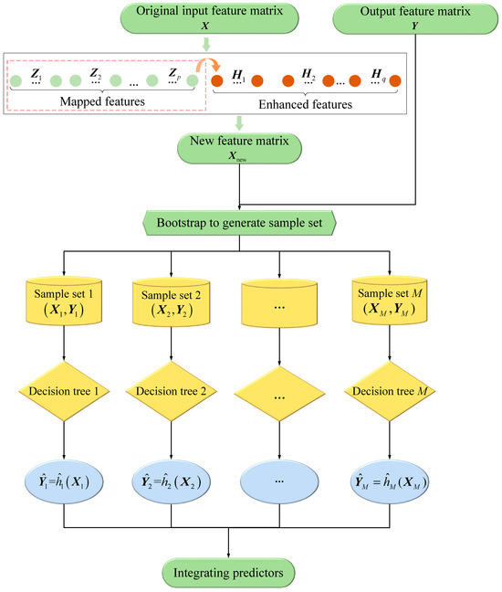
Figure 1.
The framework of BRF.
The overall calculation complexity of BRF is the sum of the complexity of feature expansion and RF, namely . The calculation complexity of the activation function is ignored.
3.2. Prediction Process
The BRF model is applied to the prediction of wind power, as illustrated in Figure 2. Specifically, the wind power prediction process is primarily divided into the following four steps.
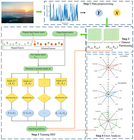
Figure 2.
Flowchart of the proposed BRF model.
- (a)
- Data preprocessing. This involves the identification and replacement of outliers, the imputation of missing values, and the normalization of the dataset.
- (b)
- Dataset partitioning. The sliding window approach is used to create training and test sets from preprocessed data.
- (c)
- Model training. The input features of the training sets are mapped and enhanced by using BLS, and the RF is trained on the new input features and the original output features.
- (d)
- Model evaluation. The BRF model is subjected to three error assessments on the test sets.
Once trained, the BRF model is used to predict the input features of the test samples. Initially, the mapping layer is employed to generate the mapping vector , where . Subsequently, the vector is enhanced to obtain the enhancement vector , where . Finally, the new features are input into the RF, resulting in the final predicted value through integration
where is denoted as the finally prediction results and refers to the prediction feature.
3.3. Comparison with Existing Work
During the process of establishing the BRF, we reviewed a variety of machine learning models to testify to the advantages of proposed model. At the same time, we also found that many existing models are relevant to our work. This subsection focuses on making a comparative explanation with relevant work.
Zhou [33] et al. explored the possibility of building deep models based on non-differentiable modules, such as decision trees, and proposed an approach that generates a deep forest holding these characteristics, named gcForest. This model adopts a cascaded structure and learns the feature information of the input feature vector through a random forest. After processing, the information is passed to the next layer. In order to enhance the generalization ability of the model, multiple different types of random forests are selected for each layer. The gcForest is derived from deep learning methods and improves the computational efficiency on the basis of deep learning. Due to multiple cross-validations, it still has a relatively high computational complexity. Therefore, this model is more suitable for classification problems rather than the wind power prediction problem discussed in this paper.
Zhan [34] et al. proposed a machine learning model for COVID-19 prediction based on the BLS. They first leveraged RF to screen out the key features and then developed a random-forest-bagging BLS (RF-Bagging-BLS) approach to forecast the trend of the COVID-19 pandemic. In this model, the RF is used to select the importance of features so as to enhance the predictive ability of the BLS. The differences between RF-Bagging-BLS and our BRF are mainly reflected in the following two aspects: (a) In BRF, the function of RF is to conduct integrated prediction rather than feature screening; (b) RF-Bagging-BLS is applicable to multivariate prediction.
Wan [35] et al. proposed a broad random forest-based multi-output soft sensor modeling method based on the idea of an attention mechanism derived from the concept of broad learning systems. While BRF is likewise constructed in [35], their methodology diverges completely from our framework. In [35], the construction of BRF is mainly completed by embedding the RF into each module of the BLS. At the feature mapping layer, feature enhancement layer, and incremental learning layer, the main function of the RF is to cooperate with the RMSE to calculate the weights. Its main architecture relies on the BLS, and only the weight calculation in the BLS is replaced with the RF to make it more objective.
However, the construction process of the BRF in this paper realizes the integration of the BLS and the RF. The key distinctions between literature [35] and our work are summarized below: (a) For the BRF proposed in this paper, the weights of the last layer are not calculated; that is, the least squares method is not used. (b) In our framework, the RF aims to predict the new dataset constructed by BLS, rather than calculating the weights. (c) The method in [35] is applicable to multivariate prediction. The construction manners of these two types of BRF are completely different, and their applications also vary greatly, so there is no comparability between them.
4. Case Study
This section presents the origins and fundamental details of the two datasets and lists parameter configurations for the models. It also delineates the assessment measures required for the experimental outcomes.
4.1. Datasets Description and Parameters Configuration
This study conducts experiments on two datasets, labeled as Dataset 1 and Dataset 2. Dataset 1 contains wind power data from Hebei Province in China for May 2018 with a sampling interval of 10 min, whereas Dataset 2 contains data from Galicia in Spain for July 2018 with a sampling period of 5 min. The two datasets were measured units of kW.
To improve data consistency, we preprocess the historical wind power series. Firstly, the outliers in the original power sequence are found using the concept. The missing and anomalous values are then corrected using a piecewise linear interpolation technique. Finally, the processed sequence is normalized within the range of 0 to 1 to mitigate the dimensional effect.
The basic statistical information of two investigated datasets is shown in Table 1, where , and represent the first, second, and third quartiles, respectively. Max, Min, Mean, and Std represent the maximum value, minimum value, mean value, and standard deviation of the data. Afterwards, each dataset is split into a training set and a test set by an 8:2 ratio.

Table 1.
Basic statistical information of two wind power datasets.
For comparison purposes, Table 2 provides the specific parameter settings of several single models including BLS, RF, extremely randomized trees (ERT), Transformer, LSTM, and SVM. The BLS module in the BRF model has the same parameter settings as single BLS. For common parameters, GRU, BiLSTM, and BiGRU have the same settings as LSTM. In SVM, the radial basis kernel is chosen as the kernel function, where tuning parameter controls the width of the function.
Table 2.
Parameter settings of single models.
4.2. Evaluation Metrics
For a one-step prediction task, we consider the following three error-evaluation metrics on the test set with n samples. These evaluation metrics are mean absolute error (MAE), root mean square error (RMSE), and coefficient of determination (R2). Their calculation formulas are as follows
where and represent respectively the actual value and the predicted value for the i-th test sample, and denotes the average of actual values.
5. Experimental Results and Analysis
5.1. Comparison and Analysis of One-Step Prediction Results
To verify the effectiveness of the proposed BRF, nine other models are developed to compare their prediction performance on two datasets. All compared models are comprised of RF, BLS, SVM, ERT, LSTM, GRU, BiLSTM, BiGRU, and Transformer.
For the aforementioned 10 models, Table 3 and Table 4 present three evaluation metrics on two datasets. As shown in Table 3, the MAE, RMSE, and R2 values of the proposed model are 134.3293 kW, 241.2171 kW, and 0.9650 on the first dataset, representing improvements of at least 3.43%, 0.94%, and 0.22% over the other 9 models. Table 4 further shows that BRF retains the best predictive accuracy on Dataset 2, with MAE, RMSE, and showing improvements of at least 3.80%, 3.34%, and 0.44%.
Table 3.
Prediction performance comparison on Dataset 1.
Table 4.
Prediction performance comparison on Dataset 2.
Due to the limited characteristics of wind power data, traditional machine learning models such as SVM, LSTM, and GRU struggle to adequately capture the nonlinear features, resulting in suboptimal forecasting performance. The BLS model enhances and maps’ existing features, effectively representing the nonlinear characteristics of the original wind power series. In contrast, the RF model randomly selects features and employs multiple decision trees in parallel, increasing operational efficiency. Among BRF, BLS, and RF, the BRF outperforms the other two models by 0.22% and 0.44% in on Dataset 1. In Dataset 2, the BRF shows improvements of 0.40% and 0.65% over BLS and RF, respectively. Consequently, the BRF achieves superior predictive performance.
5.2. Visualization of One-Step Prediction Results
The previous subsection compares three error-evaluation metrics presented in tabular form. In this subsection, we will provide a visual comparison of the prediction results. Figure 3 and Figure 4 illustrate the prediction curves of all models across two datasets, respectively.
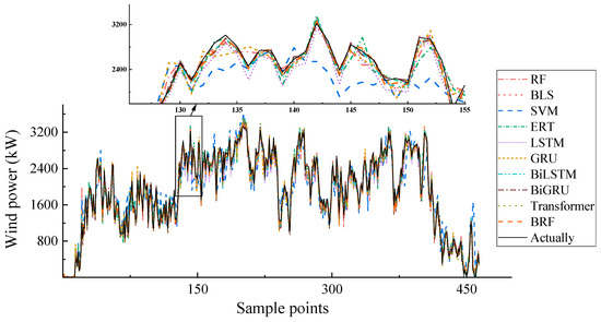
Figure 3.
Prediction results comparison on Dataset 1.
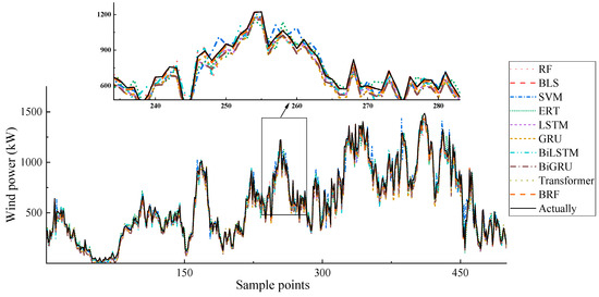
Figure 4.
Prediction results comparison on Dataset 2.
As can be seen from the figures, the predicted values of the BRF are closest to the actual values. Especially at the extreme points, the predicted values of the BRF are almost the same as the actual values. This proves that the BRF has the best prediction performance and also has good stability at the peak values.
5.3. Time Efficiency Comparison
This subsection evaluates the time efficiency of all models during the training phase for two wind power datasets. Table 5 and Table 6 present the training duration of ten models across both datasets. Figure 5 and Figure 6 visually compare the training times through histograms for two datasets and reports the average time for the 10 models.
Table 5.
Training time comparison on Dataset 1 (in seconds).
Table 6.
Training time comparison on Dataset 2 (in seconds).
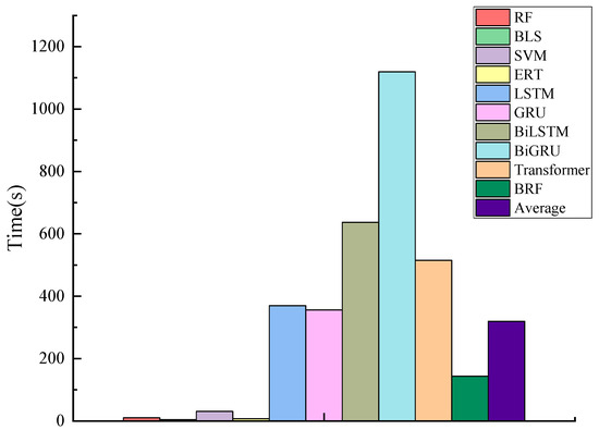
Figure 5.
Training time comparison on Dataset 1.
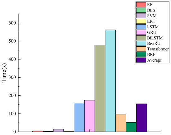
Figure 6.
Training time comparison on Dataset 2.
By observing the two tables and figures, it can be seen that both the BLS and RF models significantly enhance computational efficiency in comparison to deep learning models (i.e., GRU, LSTM, BiGRU, BiLSTM, and Transformer). This evidence implies that the architectures of BLS and RF can effectively reduce the time complexity of the models.
In summary, the time efficiency of this subsection validates that the training time required by the proposed model is significantly less than that of deep learning models and the average.
5.4. Comparison and Analysis of Multi-Step Prediction Results
Multi-step recursive forecasting is a prediction method based on the recursive mechanism of time series. Its core idea is to iteratively use the previous step’s prediction result of the model as the input for subsequent predictions and gradually generate multi-step future predicted values. The advantages of this method are mainly reflected in the following aspects. Firstly, the model architecture is lightweight. Only a single-step prediction model is required to achieve multi-step prediction, avoiding the problem of parameter inflation in complex multi-output structures. Secondly, it can dynamically adapt to the evolution of time series. By gradually updating the input features through the recursive mechanism, it can capture the non-stationarity and dynamic dependence of time series. Thirdly, it has the ability of online updating, which is suitable for streaming data scenarios, and can correct prediction errors through real-time feedback. Fourthly, it has high computational efficiency. Compared with direct multi-step forecasting, which requires independent modeling for each prediction step, the shared parameter design of recursive forecasting significantly reduces the computational complexity.
To validate the capability of BRF in capturing data characteristics over the long term, the following will conduct multi-step forecasting experiments on two datasets, including 2-step, 4-step, 6-step, and 8-step predictions. In order to understand clearly the stability of BRF, we have also selected the top four models in terms of prediction accuracy to conduct multi-step predictions. Specifically, the models for multi-step forecasting experiments include BRF, Transformer, BLS, and BiLSTM. The prediction results are shown in Table 7, Table 8, Table 9 and Table 10. Taking the of Dataset 2 as an example, the 8-step predictions of the four models have decreased 18.49%, 19.08%, 19.47%, and 19.34%, respectively, compared with the 1-step predictions. This indicates that when performing multi-step predictions, BRF has higher stability and a smaller decline. At the same time, after multi-step predictions, the prediction accuracy of BRF is still higher than that of the other three models.
Table 7.
Multi-step prediction results of the proposed BRF.
Table 8.
Multi-step prediction results of the proposed Transformer.
Table 9.
Multi-step prediction results of the proposed BLS.
Table 10.
Multi-step prediction results of the proposed BiLSTM.
It is evident that in multi-step prediction, the BRF continues to demonstrate strong predictive performance, yielding reliable outcomes that enhance the stability of the prediction system and exhibit commendable robustness.
6. Conclusions
To enhance the accuracy of wind power prediction, this paper introduces a lightweight machine learning model, namely the broad random forest (BRF). This model initially applies a broad learning system (BLS) to map and enhance existing features, and then employs random forest (RF) for prediction based on the reconstructed features. The BLS module demonstrates higher computational efficiency during the training process. Concretely speaking, its network architecture lacks the complex gradient calculations and parameter update procedures associated with the backpropagation algorithm found in deep neural networks, resulting in significantly reduced training times. Furthermore, the RF module has great prediction accuracy and good interference resistance, giving the proposed model the benefit of both high precision and robust stability. Experiments conducted on two real datasets show that the predictive performance of BRF significantly surpasses other models.
Future research could also delve into the combination of different machine learning algorithms with BRF. For instance, hybridizing BRF with neural network might bring about synergetic effects. LSTM has a remarkable ability to capture long-term dependencies in time series data, which could complement the strengths of BRF in handling complex nonlinear relationships. By integrating these two algorithms, it is possible to better analyze the sequential nature of wind power data. However, this model also has certain limitations. For example, it cannot accurately select the optimal parameter settings. In the future, it can be combined with intelligent optimization algorithms to make the parameter selection more optimal and the model accuracy higher.
In addition, the use of more comprehensive and accurate data sources should be emphasized. Instead of solely relying on historical wind power generation data, incorporating meteorological data from multiple reliable sources, such as high-resolution numerical weather prediction models, could provide a more complete picture of the factors influencing wind power. This would enable a more in-depth understanding of the complex interactions between various meteorological elements and wind power generation, thus facilitating the development of more accurate prediction models.
As a core enabling element of the new power system, wind power forecasting technology has reconstructed the sustainable paradigm for the development of renewable energy through a multi-dimensional collaborative mechanism. At the system operation level, by means of time-series feature decoupling and a probabilistic forecasting framework, it effectively resolves the contradiction between the randomness of wind power and the rigid scheduling of the power grid, laying a technical foundation for the grid connection of a high proportion of renewable energy. At the level of technological innovation, the integrated application of meteorological mode decomposition and deep reinforcement learning accelerates the digitalization process of energy. Under the triple constraints of energy security, economic feasibility, and environmental sustainability, it opens up a Pareto-optimal path for the high-quality development of clean energy.
Author Contributions
Writing—original draft preparation, Y.C.; writing—review and editing, J.S. All authors have read and agreed to the published version of the manuscript.
Funding
Independent Research and Development project of State Key Laboratory of Green Building (LSZZ-Y202414).
Institutional Review Board Statement
Not applicable.
Informed Consent Statement
Not applicable.
Data Availability Statement
Data are unavailable due to privacy or ethical restrictions.
Conflicts of Interest
The authors declare no conflicts of interest.
References
- Qiu, H.; Shi, K.; Wang, R.; Zhang, L.; Liu, X.; Cheng, X. A novel temporal–spatial graph neural network for wind power forecasting considering blockage effects. Renew. Energy 2024, 227, 120499. [Google Scholar] [CrossRef]
- Peng, X.; Li, Y.; Tsung, F. A graph attention network with spatio-temporal wind propagation graph for wind power ramp events prediction. Renew. Energy 2024, 236, 121280. [Google Scholar] [CrossRef]
- Bashir, T.; Wang, H.; Tahir, M.; Zhang, Y. Wind and solar power forecasting based on hybrid CNN-ABiLSTM, CNN-transformer-MLP models. Renew. Energy 2025, 239, 122055. [Google Scholar] [CrossRef]
- Deng, J.; Xiao, Z.; Zhao, Q.; Zhan, J.; Tao, J.; Liu, M.; Song, D. Wind turbine short-term power forecasting method based on hybrid probabilistic neural network. Energy 2024, 313, 134042. [Google Scholar] [CrossRef]
- Ge, C.; Yan, J.; Zhang, H.; Li, Y.; Wang, H.; Liu, Y. Joint short-term power forecasting of hydro-wind-photovoltaic considering spatiotemporal delay of weather processes. Renew. Energy 2024, 237, 121679. [Google Scholar] [CrossRef]
- Li, J.; Jia, L.; Zhou, C. Probability density function based adaptive ensemble learning with global convergence for wind power prediction. Energy 2024, 312, 133573. [Google Scholar] [CrossRef]
- Wang, D.; Yang, M.; Zhang, W.; Ma, C.; Su, X. Short-term power prediction method of wind farm cluster based on deep spatiotemporal correlation mining. Appl. Energy 2024, 380, 125102. [Google Scholar] [CrossRef]
- Yang, M.; Guo, Y.; Huang, T.; Fan, F.; Ma, C.; Fang, G. Wind farm cluster power prediction based on graph deviation attention network with learnable graph structure and dynamic error correction during load peak and valley periods. Energy 2024, 312, 133645. [Google Scholar] [CrossRef]
- Zhu, Y.; Liu, Y.; Wang, N.; Zhang, Z.; Li, Y. Real-time error compensation transfer learning with echo state networks for enhanced wind power prediction. Appl. Energy 2025, 379, 124893. [Google Scholar] [CrossRef]
- Lu, P.; Yang, J.; Ye, L.; Zhang, N.; Wang, Y.; Di, J.; Gao, Z.; Wang, C.; Liu, M. A novel adaptively combined model based on induced ordered weighted averaging for wind power forecasting. Renew. Energy 2024, 226, 120350. [Google Scholar] [CrossRef]
- Camal, S.; Girard, R.; Fortin, M.; Touron, A.; Dubus, L. A conditional and regularized approach for large-scale spatiotemporal wind power forecasting. Sustain. Energy Technol. Assess. 2024, 65, 103743. [Google Scholar] [CrossRef]
- Arooj, Q. FedWindT: Federated learning assisted transformer architecture for collaborative and secure wind power forecasting in diverse conditions. Energy 2024, 309, 133072. [Google Scholar] [CrossRef]
- Zhao, Y.; Zhao, Y.; Liao, H.; Pan, S.; Zheng, Y. Interpreting LASSO regression model by feature space matching analysis for spatio-temporal correlation based wind power forecasting. Appl. Energy 2025, 380, 124954. [Google Scholar] [CrossRef]
- Wang, Y.; Zhao, K.; Hao, Y.; Yao, Y. Short-term wind power prediction using a novel model based on butterfly optimization algorithm-variational mode decomposition-long short-term memory. Appl. Energy 2024, 366, 123313. [Google Scholar] [CrossRef]
- Chen, J.; Fu, X.; Zhang, L.; Shen, H.; Wu, J. A novel offshore wind power prediction model based on TCN-DANet-sparse transformer and considering spatio-temporal coupling in multiple wind farms. Energy 2024, 308, 132899. [Google Scholar] [CrossRef]
- Yang, Y.; Wang, Z.; Zhao, S.; Zhou, H.; Wu, J. Robust autoregressive bidirectional gated recurrent units model for short-term power forecasting. Eng. Appl. Artif. Intell. 2024, 138, 109453. [Google Scholar] [CrossRef]
- Yu, M.; Tao, B.; Li, X.; Liu, Z.; Xiong, W. Local and long-range convolutional LSTM network: A novel multi-step wind speed prediction approach for modeling local and long-range spatial correlations based on ConvLSTM. Eng. Appl. Artif. Intell. 2023, 130, 107613. [Google Scholar] [CrossRef]
- Du, R.; Chen, H.; Yu, M.; Li, W.; Niu, D.; Wang, K.; Zhang, Z. 3DTCN-CBAM-LSTM short-term power multi-step prediction model for offshore wind power based on data space and multi-field cluster spatio-temporal correlation. Appl. Energy 2024, 376, 124169. [Google Scholar] [CrossRef]
- Yu, C.; Li, Y.; Chen, Q.; Lai, X.; Zhao, L. Matrix-based wavelet transformation embedded in recurrent neural networks for wind speed prediction. Appl. Energy 2022, 324, 119692. [Google Scholar] [CrossRef]
- Barjasteh, A.; Ghafouri, S.H.; Hashemi, M. A hybrid model based on discrete wavelet transform (DWT) and bidirectional recurrent neural networks for wind speed prediction. Eng. Appl. Artif. Intell. 2024, 127, 107340. [Google Scholar] [CrossRef]
- Liu, L.; Liu, J.; Ye, Y.; Liu, H.; Chen, K.; Li, D.; Dong, X.; Sun, M. Ultra-short-term wind power forecasting based on deep Bayesian model with uncertainty. Renew. Energy 2023, 205, 598–607. [Google Scholar] [CrossRef]
- Hou, G.; Li, Q.; Huang, C. Spatiotemporal forecasting using multi-graph neural network assisted dual domain transformer for wind power. Energy Convers. Manag. 2025, 325, 119393. [Google Scholar] [CrossRef]
- Qiu, L.; Ma, W.; Feng, X.; Dai, J.; Dong, Y.; Duan, J.; Chen, B. A hybrid PV cluster power prediction model using BLS with GMCC and error correction via RVM considering an improved statistical upscaling technique. Appl. Energy 2024, 359, 122719. [Google Scholar] [CrossRef]
- Zhang, L.; Zhu, J.; Zhang, D.; Liu, Y. An incremental photovoltaic power prediction method considering concept drift and privacy protection. Appl. Energy 2023, 351, 121919. [Google Scholar] [CrossRef]
- Hu, S.; Xu, X.; Li, M.; Shi, P.; Li, R.; Wang, S. Incremental forecaster using C–C algorithm to phase space reconstruction and broad learning network for short-term wind speed prediction. Eng. Appl. Artif. Intell. 2024, 128, 107461. [Google Scholar] [CrossRef]
- Liu, Y.; Li, Y.; Huang, G.; Lv, J.; Zhai, X.; Li, Y.; Zhou, B. Development of an integrated model on the basis of GCMs-RF-FA for predicting wind energy resources under climate change impact: A case study of Jing-Jin-Ji region in China. Renew. Energy 2023, 219, 119547. [Google Scholar] [CrossRef]
- Zhang, C.; Tao, Z.; Xiong, J.; Qian, S.; Fu, Y.; Ji, J.; Nazir, M.S.; Peng, T. Research and application of a novel weight-based evolutionary ensemble model using principal component analysis for wind power prediction. Renew. Energy 2024, 232, 121085. [Google Scholar] [CrossRef]
- Zheng, Y.; Chen, B.; Wang, S.; Wang, W. Broad learning system based on maximum correntropy criterion. IEEE Trans. Neural Networks Learn. Syst. 2021, 32, 3083–3097. [Google Scholar] [CrossRef]
- Deng, Z.; Chan, S.H.; Chen, Q.; Liu, H.; Zhang, L.; Zhou, K.; Tong, S.; Fu, Z. Efficient degradation prediction of PEMFCs using ELM-AE based on fuzzy extension broad learning system. Appl. Energy 2023, 331, 120385. [Google Scholar] [CrossRef]
- Chu, F.; Liang, T.; Chen, C.L.P.; Wang, X.; Ma, X. Compact broad learning system based on fused lasso and smooth lasso. IEEE Trans. Cybern. 2024, 54, 435–448. [Google Scholar] [CrossRef]
- Delgado-Panadero, Á.; Benítez-Andrades, J.A.; García-Ordás, M.T. A generalized decision tree ensemble based on the neural networks architecture: Distributed gradient boosting forest (DGBF). Appl. Intell. 2023, 53, 22991–23003. [Google Scholar] [CrossRef]
- Du, P.; Gong, X.; Han, B.; Zhao, X. Carbon-neutral potential analysis of urban power grid: A multi-stage decision model based on RF-DEMATEL and RF-MARCOS. Expert Syst. Appl. 2023, 234, 121026. [Google Scholar] [CrossRef]
- Zhou, Z.H.; Feng, J. Deep forest. Natl. Sci. Rev. 2019, 6, 74–86. [Google Scholar] [CrossRef] [PubMed]
- Zhan, C.; Zheng, Y.; Zhang, H.; Wen, Q. Random-forest-bagging broad learning system with applications for COVID-19 pandemic. IEEE Internet Things J. 2021, 8, 15906–15918. [Google Scholar] [CrossRef]
- Wan, Y.; Liu, D.; Ren, J.-C. A modeling method of wide random forest multi-output soft sensor with attention mechanism for quality prediction of complex industrial processes. Adv. Eng. Inform. 2024, 59, 102255. [Google Scholar] [CrossRef]
Disclaimer/Publisher’s Note: The statements, opinions and data contained in all publications are solely those of the individual author(s) and contributor(s) and not of MDPI and/or the editor(s). MDPI and/or the editor(s) disclaim responsibility for any injury to people or property resulting from any ideas, methods, instructions or products referred to in the content. |
© 2025 by the authors. Licensee MDPI, Basel, Switzerland. This article is an open access article distributed under the terms and conditions of the Creative Commons Attribution (CC BY) license (https://creativecommons.org/licenses/by/4.0/).