Analysis of Influencing Factors of Terrestrial Carbon Sinks in China Based on LightGBM Model and Bayesian Optimization Algorithm

Abstract

With accelerating climate change and urbanization, regional carbon balance faces increasing uncertainty. Terrestrial carbon sinks play a crucial role in advancing China’s sustainable development under the dual-carbon strategy. This study quantitatively modeled China’s terrestrial carbon sink capacity and analyzed the multidimensional relationships between impact factors and carbon sinks. After preprocessing multi-source raster data, we introduced kernel normalized the difference vegetation index (kNDVI) to the Carnegie–Ames–Stanford approach (CASA) model, together with a heterotrophic respiration (R_h) empirical equation, to simulate pixel-level net ecosystem productivity (NEP) across China. A light gradient-boosting machine (LightGBM) model, optimized via Bayesian algorithms, was trained to regress NEP drivers, categorized into atmospheric components (O₃, NO₂, and SO₂) and subsurface properties (a digital elevation model (DEM), enhanced vegetation index (EVI), soil moisture (SM)), and human activities (land use/cover change (LUCC), POP, gross domestic product (GDP)). Shapley Additive Explanation (SHAP) values were used for model interpretation. The results reveal significant spatial heterogeneity in NEP across geographic and climatic contexts. The pixel-level mean and total NEP in China were 268.588 gC/m²/yr and 2.541 PgC/yr, respectively. The north tropical zone (NRZ) exhibited the highest average NEP (828.631 gC/m²/yr), while the middle subtropical zone (MSZ) and south subtropical zone (SSZ) demonstrated the most stable NEP distributions. LightGBM achieved high simulation accuracy, further enhanced by Bayesian optimization. SHAP analysis identified EVI as the most influential factor, followed by SM, NO₂, DEM, and POP. Additionally, LightGBM effectively captured nonlinear relationships and variable interactions.

1. Introduction

The carbon balance is undergoing significant shifts due to climate change, posing a threat to ecosystem sustainability [1]. The regulation of ecosystem carbon sinks is considered to be the most comprehensive and effective pathway to address carbon-neutral governance. The carbon sink is the result of the carbon cycle and reflects the relative magnitude of carbon emissions and carbon sequestration, revealing the carbon balance state of the ecosystem. Among the various ecosystem components, terrestrial ecosystems are the component with the greatest uncertainty in the calculation under the background of urbanization expansion and climate change intensification [2,3,4], and show potential in the carbon uptake [5,6,7]. Understanding the carbon sinks at a regional scale and characterizing the role of influencing factors can provide a scientific basis for carbon management decisions in the context of carbon peaking and carbon neutrality goals. However, the carbon balance of terrestrial ecosystems under different climatic contexts is still unclear, while the influence mechanism of carbon sinks under the effect of multiple factors needs to be further refined.

The carbon cycle involves multiple inter-related concepts, including gross primary productivity (GPP), net primary productivity (NPP), net ecosystem productivity (NEP), and net biome productivity (NBP), while NEP serves as a direct indicator of the carbon sink [3]. Carbon sink estimation methods fall into four main categories [3,4,8]: ground inventory-based accounting [9], top-down inversion [10], eddy covariance measurements [11], and model simulations [12,13]. Each of these methods has its own advantages, but in consideration of their constraints, inventory-based methods are limited by high labor costs and lack temporal continuity. Inversion methods, suited for global assessments, are constrained by a coarse data resolution. Eddy covariance provides carbon exchange measurements based on micrometeorology principles from specific sites, with professional knowledge on the data process and quality control required. In contrast, model simulations are preferred for medium- to large-scale regional studies due to their scalability and spatial continuity. In addition, the development of data-driven methods in recent years has gradually been integrated with traditional computational methods, bringing new possibilities for carbon sink simulations. In this case, data of a high quality and sufficient quantity are required.

Among all these methods, the Carnegie–Ames–Stanford approach (CASA) model [14,15] is widely used and adopted in this study due to its mechanistic depth, data availability, and computational efficiency [16,17]. As a light energy utilization model driven by meteorological and remote sensing data, it incorporates vegetation physiological processes, making it a reliable tool for productivity simulation. Traditionally, the normalized difference vegetation index (NDVI) serves as a key vegetation index in CASA; however, recent studies have highlighted its susceptibility to canopy background brightness variations [18] and inaccuracies in soil background processing [19,20]. To address these limitations, the kernel normalized difference vegetation index (kNDVI), a refined vegetation index [20], has been developed, offering greater stability, robustness, and improved spectral information utilization and has been involved in the application of vegetation expression [21]. Its superior adaptability under diverse environmental conditions makes it particularly suitable for productivity modeling [22,23]. Therefore, in this study, the kNDVI replaces the NDVI as an input parameter in the CASA, exploring its appliance for integrating into the model simulation about productivity expression.

Carbon sinks are influenced by a wide range of factors from different scales and perspectives, reflecting complex mechanism characteristics. Meteorological factors most directly provide the hydrothermal and light conditions for photosynthesis. Atmospheric components will influence plant productivity and respiration through air pollution and climate feedbacks. Subsurface properties relate to regulating vegetation growth and soil carbon processes. Human activities and disturbances will introduce interferences that significantly alter carbon sequestration and emissions.

When conducting research on factors affecting carbon sinks, factors are often selected from the above dimensions in combination with representativeness and data availability to meet different research needs and the depth of analysis of the driving mechanism. Zhao et al. [24] selected the vapor pressure deficit (VPD), temperature, solar surface downward radiation (SSRD), precipitation, soil moisture, and cloudiness as the key influencing factors of GPP, and used correlation analyses to explore the response to meteorological factors as well as the Lindeman–Merenda–Gold (LMG) method to explore the driving mechanisms of GPP. Hasi et al. [25] explored the characteristics of the roles of the soil moisture, temperature, and N effectiveness in regulating carbon exchange in meadow grassland ecosystems and emphasized the importance of the volumetric soil water content (VWC) in ecosystem carbon exchange. Huang et al. [26] quantified the land use/cover change (LUCC) trajectories and explored the impacts of climate change, CO₂ fertilization effects, and the contribution of LUCC to the global NEP based on the scenario analysis method with process model parameter control. A comprehensive selection of drivers will enhance the macro-level understanding of carbon sink dynamics, providing theoretical support for a targeted policy formulation, but it is faced with the challenge of balancing the completeness and accuracy of the data collection.

Different regression models have been applied in illustrating relationships between carbon sinks and impact factors. Lyu et al. [27] used residual analysis to quantitatively isolate anthropogenic disturbances to vegetation change from the interactive effects of human activities and climate change, and ultimately found that the contributions of climate change and anthropogenic activities to vegetation dynamics were 64.16% and 35.84%, respectively. The limitation of this method is that it cannot separate the contributions of specific influencing factors in a more detailed way and, moreover, it will generalize the joint effect of multiple factors to a single factor. Yang et al. [28] used ridge regression to analyze the influence mechanism of NEP in karst landscapes by selecting multiple factors with a comprehensive consideration of climatic, hydrological, and drought conditions and found that among all the factors, the drought fluorescence monitoring index (DFMI) they constructed was the main driver of the interannual and rainy season NEP in Asian karst concentrated distribution area (AKC) with relative contributions of 38.05% and 32.82%, respectively. Huang et al. [29] used Partial Least Squares Structural Equation Modeling (PLS-SEM) to explore the mechanisms by which LUCC, forest age, climate data, and CO₂ drive NEP and to quantify the factor interactions. Pang et al. [30] considered the influence of natural environmental and socio-economic factors on NEP within the urban agglomerations in the middle reaches of the Yangtze River, and used geographically and temporally weighted regression (GTWR) models to explore the mechanisms driving the carbon sinks, emphasizing spatio-temporal heterogeneity. However, most of these regression models are based on the traditional linear fitting principle, which cannot reveal the non-linear relationships between the factors and carbon sink.

At the same time, the emergence and development of machine learning technology provides the possibility of capturing the nonlinear relationship between variables in regression analysis. According to different learning tasks, a variety of machine learning models have been developed for classification, clustering, regression, dimensionality reduction, etc., showing great advantages in the data processing capability and complex problem solving. The Light Gradient-Boosting Machine (LightGBM) is a recently developed algorithm that performs well in terms of its speed, accuracy, and robustness. As a type of classical ensembled model working on boosting, LightGBM works by building reliable models in a sequential manner through a set of weak learners (in particular, decision trees) to provide comprehensive insights into the data. Compared with other machine learning models, LightGBM combines the explicit specification of the overfitting term with advantages in the training speed, accuracy, and generalization ability.

Optimizing hyperparameters and enhancing the model interpretability are critical for improving the performance of LightGBM models. Traditional tuning methods, such as a grid search or random search, are inefficient in high-dimensional parameter spaces and prone to local optima. In contrast, Bayesian optimization [31] efficiently explores hyperparameter combinations, significantly enhancing the model accuracy and computational efficiency. On the other side, interpretability still remains a key challenge, as machine learning models operate as black boxes. It has been pointed out that the performance of machine learning techniques is inversely proportional to the interpretability [32]. To address this, SHAP (Shapley Additive Explanations) [33,34] quantify the marginal contribution of each feature, providing a transparent and widely adopted approach for understanding machine learning’s decision-making process. ZHOU et al. [35] used a LightGBM model integrated with GridSearchCV optimization to predict and attribute carbon emissions from buildings and combined it with SHAP values for the model interpretation. Yi et al. [36] explored the relationship between NPP and socio-economic development (SDE) based on more than 10 machine learning models using county-level statistics in China, and used SHAP to explain the relationship between each influencing factor and NPP in the optimal-performing XGBOOST model from global to local aspects. Zhou S et al. [37] used Bayesian-Optimized LightGBM for the assessment of urban flood risk and vulnerability, and introduced SHAP values for multi-factor decoupling analysis.

The power and application potential demonstrated by machine learning in data processing has begun to be combined and applied in the environmental field in recent years, like flood risk assessment [37], thermal environment analysis [38,39], air pollutant forecasting [40], and so on. In carbon-related studies, the main focus is on carbon flux prediction [41,42]. Prăvălie et al. [43] implemented NPP modeling based on dozens of multi-machine learning techniques on a national scale for Romania by grasping the trend evolution characteristics of the NPP combined with multi-source data including remotely sensed data and inventory data. However, the application of machine learning techniques, especially the LightGBM model, to the carbon sink driving mechanism has yet to be further explored.

The objective of this study is to reveal the state and influencing characteristics of the carbon balance state in China. More specifically, the CASA model and heterotrophic respiration (R_h) empirical equation were applied for NEP simulation. Further, the novel vegetation index kNDVI was introduced into the CASA calculation session for model enhancement. To obtain a more comprehensive understanding of the influencing mechanism of the carbon sink, the LightGBM algorithm was used coupled with the Bayesian Optimization algorithm to find the best hyperparameter set. Finally, the SHAP value was used to explain the model training result between terrestrial carbon sinks and their variables in China. Through the above analysis, the influencing characteristics of carbon sinks will be obtained in China. The results of this study might provide some theoretical basis for the sustainable and low-carbon development policies.

2. Materials and Methods

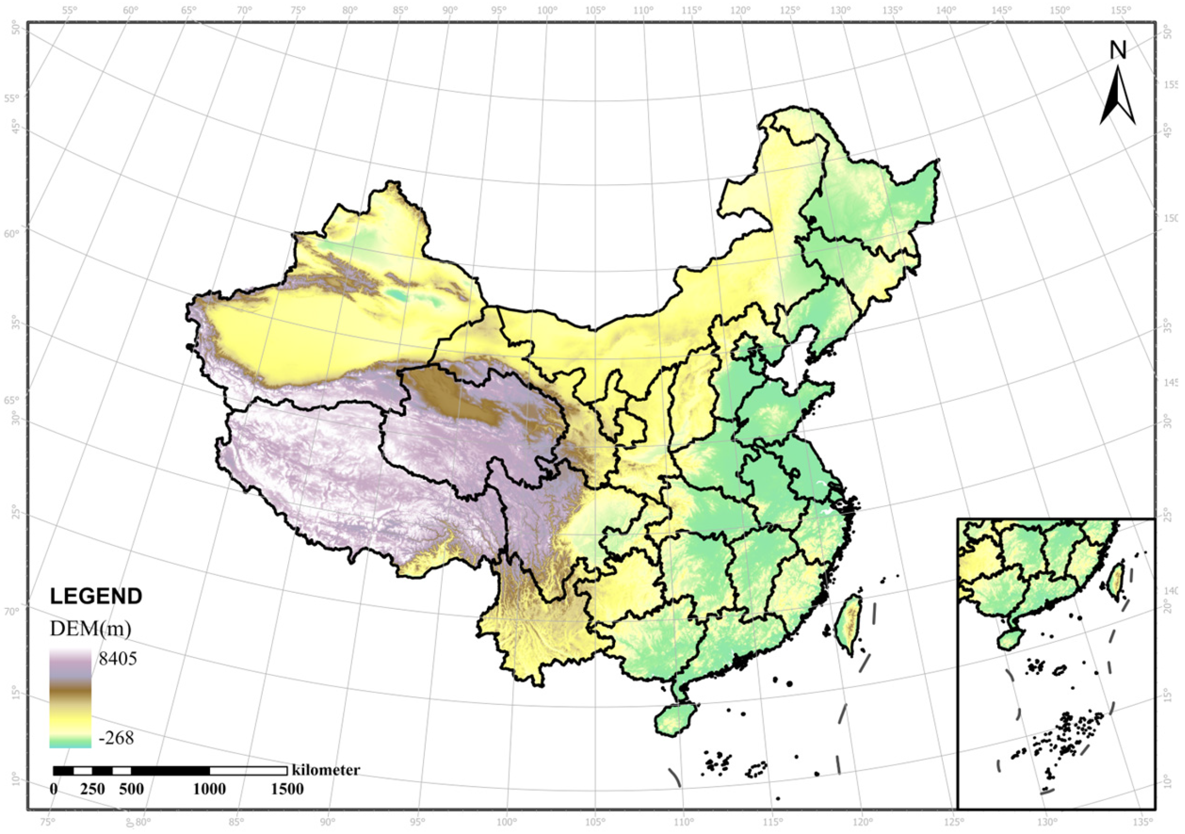
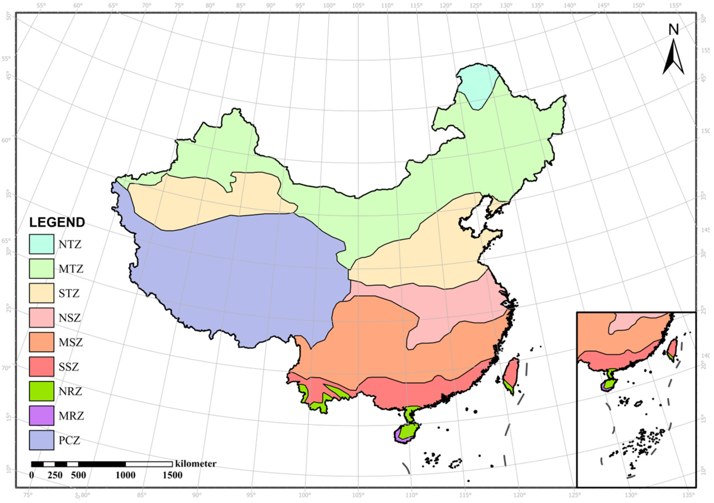
2.1. Research Area

China (73°33′ E–135°05′ E, 3°51′ N–53°33′ N) exhibits a complex topography and diverse climatic conditions. The terrain follows a three-step gradient from west to east, with average elevations decreasing from 4000 m to 1000 m to 500 m, alongside a forest–steppe–desert continuum from southeast to northwest. Climatically, a humid–semiarid–arid transition emerges from the southeastern coast to the northwestern interior. Additionally, contrasting population densities and urbanization-driven human activities further complicate spatial and temporal distribution and driving mechanisms of carbon sinks across regions. Figure 1 shows the distribution of provincial boundaries in China on the map of digital elevation model (DEM), and Figure 2 shows the distribution of the climatic zoning boundaries used in this study.

2.2. Data Resource

Table 1. Summary table for data resources in this study.

Usage in Study	Data Type	Accuracy Indicators	Original Resolution	Dataset Resource	Download Platform
NEP calculation section	Precipitation	-	0.008333°, monthly	Peng, et al. [45]	geodata, accessed on 30 August 2023, https://www.geodata.cn/
	Temperature	-	0.008333°, monthly	Peng, et al. [45]	geodata, accessed on 2 September 2023, https://www.geodata.cn/
	NDVI	-	1 km × 1 km, monthly	MOD 13Q1, MODIS	geodata, accessed on 15 September 2023, https://www.geodata.cn/
	Landcover	-	30 m, yearly	CLCD [46]	zenodo, accessed on 22 June 2024, https://zenodo.org/records/8176941
	Radiation	-	10 km × 10 km, hourly	ERA5 LAND [47]	GEE, accessed on 2 July 2024, https://developers.google.com/earth-engine/
Influencing factors analysis section	Population, POP	-	1 km × 1 km, yearly	Xu [48]	RESDC, accessed on 3 March 2024, http://www.resdc.cn
	Gross Domestic Product, GDP	-	1 km × 1 km, yearly	Xu [49]	RESDC, accessed on 2 March 2024, http://www.resdc.cn
	Sulfur Dioxide, SO2	CV-R2: 0.84, RMSE: 10.07 μg/m3, MAE: 4.68 μg/m3	1 km × 1 km, netCDF, yearly	CHAP [50]	geodata, accessed on 30 August 2024, https://www.geodata.cn/
	Nitrogen Dioxide, NO2	CV-R2: 0.93, RMSE: 4.89 μg/m3, MAE: 3.48 μg/m3	1 km × 1 km, netCDF, yearly	CHAP [51]	geodata, accessed on 30 August 2024, https://www.geodata.cn/
	Ozone, O3	CV-R2: 0.89; RMSE: 15.77 µg/m3; MAE: 10.48 mg/m3	1 km × 1 km, netCDF, yearly	Wei, et al. [52]	geodata, accessed on 30 August 2024, https://www.geodata.cn/
	Soil Moisture	ubRMSE: 0.045–0.051, 0.041–0.052; R2: 0.866–0.893, 0.883–0.919	1 km × 1 km, daily, netCDF type	SMCI1.0 [53]	The China’s National Tibetan Plateau Data Center, accessed on 31 August 2024.
	Enhanced Vegetation Index, EVI	-	1 km × 1 km, yearly	MOD13Q1, MODIS	RESDC, accessed on 7 November 2024, http://www.resdc.cn
	Digital Elevation Model, DEM	resampled based on the latest SRTM V4.1 radar image to the spatial resolution of 1 km	1 km × 1 km, yearly	original SRTM V4.1	RESDC, accessed on 7 November 2024, http://www.resdc.cn

(MODIS: Moderate-resolution Imaging Spectroradiometer, CLCD: China Land Cover Dataset, GEE: Google Earth Engine, CHAP: China High Air Pollutants, SMCI: Soil Moisture of China by in situ data, version 1.0, SRTM: Shuttle Radar Topography Mission).

offers information and resources of data used in this study. All input data are processed with the transformation and correction including resampling, reprojection, mask extraction, raster calculation, band synthesis, etc., through ArcgisPro 3.0.2 and programming language (Rstudio 4.3.3, python 3.11, and arcpy (based on Python 3)). Our goal is to obtain the matched settings for the input data with the same details like the number of rows and columns, spatial range, and temporal scope to meet the needs of the model operation and the subsequent calculation and analysis work.

2.3. Methods

2.3.1. CASA Model

In this study, CASA model was used for NPP simulation, which is an improved version of the algorithm proposed by Zhu [54] with the introduction of the vegetation classification accuracy as well as the FPAR combination. It has been continuously and widely used [16,17,55,56] due to its mechanistic insights, data convenience, and availability.

NPP relates to the biomass state for the vegetation and takes up a certain percentage of GPP. In CASA model, NPP is derived through the two parts below for calculation at pixel-scale.

$$NP{P}_{\left(x,t\right)}=APA{R}_{\left(x,t\right)}\times {\epsilon }_{\left(x,t\right)},$$

(1)

where APAR_(x,t) denotes photosynthetically active radiation absorbed for pixel x in month t (MJ·m⁻² ·month⁻¹ ); ε_(x,t) is the actual light energy utilization efficiency for pixel x in month t (gC MJ⁻¹ ).

The calculation method of APAR is as follows:

$$APA{R}_{\left(x,t\right)}=SO{L}_{\left(x,t\right)}\times FPA{R}_{\left(x,t\right)}\times 0.5,$$

(2)

where SOL_(x,t) is total solar radiation (MJ · m²) for pixel x in month t; FPAR is the proportion of photosynthetically active radiation absorbed by the vegetation layer; and 0.5 is the constant of the proportion of effective photosynthetic radiation that can be absorbed and utilized by the vegetation layer, which relates to the portion of band length with the range of 0.38–0.71 μm in the total solar radiation.

FPAR(x,t), standing for the value in each pixel, needs to be weighted by two parameters, FPAR_NDVI and FPAR_SR, which are calculated with NDVI and SR based on Equation (4) and Equation (5), respectively.

$$FPA{R}_{\left(x,t\right)}=\alpha FPA{R}_{NDVI}+\left(1-\alpha \right)FPA{R}_{SR},$$

(3)

$$FPA{R}_{NDVI}={\displaystyle \frac{NDV{I}_{\left(x,t\right)}-NDV{I}_{\left(i,min\right)}}{NDV{I}_{\left(i,max\right)}-NDV{I}_{\left(i,min\right)}}}\times \left(FPA{R}_{max}-FPA{R}_{min}\right)+FPA{R}_{min},$$

(4)

$$FPA{R}_{SR}={\displaystyle \frac{S{R}_{\left(x,t\right)}-S{R}_{\left(i,min\right)}}{S{R}_{\left(i,max\right)}-S{R}_{\left(i,min\right)}}}\times \left(FPA{R}_{max}-FPA{R}_{min}\right)+FPA{R}_{min},$$

(5)

$$S{R}_{\left(x,t\right)}={\displaystyle \frac{1+NDV{I}_{\left(x,t\right)}}{1-NDV{I}_{\left(x,t\right)}}},$$

(6)

where NDVI_i,max is the NDVI value calculated after combining the vegetation classification accuracy with the probability distribution to characterize the full-coverage state, while NDVI_i,min uses the lower 5% quartile of NDVI in sparsely vegetated areas (e.g., bare ground, desert). FPAR_min and FPAR_max denote constants independently of vegetation type, taking values of 0.001 and 0.95, respectively. SR denotes the ratio vegetation index and is derived upon NDVI based on Equation (6), while SR _(i,min) and SR _(i,max) were calculated using the lower 5% and 95% quantiles of NDVI values for vegetation type i with Equation (6). α denotes the adjustment factor calculated by the combination of the two FPAR formulas, which was taken as 0.5 in this study.

The calculation of the ε_(x,t) consists of the following components:

$${\epsilon }_{\left(x,t\right)}=T_{\epsilon 1\left(x,t\right)}\times T_{\epsilon 2\left(x,t\right)}\times W_{\epsilon \left(x,t\right)}\times {\epsilon }_{max},$$

(7)

T_ε1(x,t) and T_ε2(x,t) denote the dimensionless coefficients reflecting the low-temperature and high-temperature stress effects on the vegetation layer, respectively. W_ε(x,t) reflects the stress effect of the environmental moisture condition where the vegetation layer is located. ε_max characterizes the maximum light energy utilization (gC/MJ) that the vegetation layer can achieve under ideal conditions.

The calculation for the stress coefficients is presented as below.

$$T_{\epsilon 1\left(x,t\right)}=0.8+0.02\times T_{opt\left(x\right)}-0.0005\times {\left[T_{opt\left(x\right)}\right]}^2,$$

(8)

$$\begin{gathered} T_{\epsilon 2\left(x,t\right)}={\displaystyle \frac{1.184}{\left\{1+\exp \left[0.2\times \left(T_{opt\left(x\right)}-10-T_{\left(x,t\right)}\right)\right]\right\}}} \\ \times {\displaystyle \frac{1}{\left\{1+\exp \left[0.3\times \left(-T_{opt\left(x\right)}-10+T_{opt\left(x\right)}\right)\right]\right\}}}, \end{gathered}$$

(9)

$$W_{\epsilon \left(x,t\right)}=0.5+0.5\times E_{\left(x,t\right)}/E_{p\left(x,t\right)},$$

(10)

The temperature stress factor reflects the inhibitory effect on photosynthesis by internal biochemistry of vegetation under high and low temperatures, and is calculated from the optimum temperature T_opt(x). Moisture stress factor reflects the effect of vegetation’s ability to utilize the effective moisture of the environment on photosynthesis, which was calculated based on the ratio of the actual evapotranspiration of the region E_(x,t) and the potential evapotranspiration of the region E_p(x,t), which was set to be calculated based on the precipitation and the atmospheric temperature in the present model. ε_max was determined based on the literature collection. The detailed and specific expansion and descriptions for the unexpanded formulas can be found in ZHU’s proposal.

2.3.2. kNDVI

The kernel NDVI (kNDVI) is a novel type of vegetation index improved on the basis of NDVI [20], which maximizes the use of spectral information and demonstrates greater stability and robustness in productivity fitting under different environmental conditions. The kNDVI values were obtained by mapping transformation and smoothing of the NDVI values with nonlinear kernel functions via hyperbolic tangent function. It has already been applied to numerous research [21,22,23,57] in recent years.

$$kNDVI=\tanh \left\{{\left({\displaystyle \frac{NIR-red}{2\sigma }}\right)}^2\right\}=\tanh \left(NDV{I}^2\right),$$

(11)

where NIR and red refer to reflectance in the near-infrared and red bands, respectively, and σ denotes the length-scale parameter taken as 0.5 to indicate the average of NIR and red bands.

2.3.3. R_h Empirical Model

Referring to the previous study [58,59], the formula for calculating heterotrophic respiration is as follows:

$$R_h=3.069\left({\mathrm{e}}^{0.0912\cdot T}+ln\left(0.3145\cdot R+1)\right.\right),$$

(12)

where T is the average atmospheric temperature (°C) and R denotes total precipitation (mm). The outcome R_h is expressed in gC·m⁻². Note that the parameters in the formula should meet the same temporal scale, so the yearly R_h was obtained by the above equation after the aggregation transformation from monthly input.

2.3.4. NEP Calculation

NEP should be calculated by NPP minus heterotrophic respiration (R_h), indicating net CO₂ exchange.

$$NEP=NPP-R_h,$$

(13)

where NEP stands for net ecosystem productivity; NPP stands for net primary productivity; and $R_h$ stands for heterotrophic respiration. When NEP calculation result is above 0, it is considered to be a carbon sink state; when NEP < 0, it is determined to be a carbon source state. If NEP is exactly equal to 0, it means that the system is in a carbon equilibrium state at this time.

2.3.5. Pearson Correlation

The Pearson correlation coefficient is a common statistical method used to quantify the strength and direction of a linear relationship between two variables, calculated using the covariance of the two variables divided by the product of their respective standard deviations.

$$r={\displaystyle \frac{cov\left(x,y\right)}{{\sigma }_x{\sigma }_y}}={\displaystyle \frac{\sum \left(x-\overline{x}\right)\left(y-\overline{y}\right)}{\sqrt{\sum {\left(x-\overline{x}\right)}^2\sum {\left(y-\overline{y}\right)}^2}}},$$

(14)

The coefficient r ranges from [−1, 1] and the value of r points to the positive or negative relationship between the two variables. The closer the absolute value of r is to 1, the stronger the linear relationship between the two variables is, while the closer the absolute value to 0 signals a weaker linear relationship. When r = 0, it means that there is no linear correlation between the two variables.

2.3.6. VIF Test

The variance inflation factor (VIF) test is a measure of the severity of multicollinearity among the variables in a multiple regression task, characterized by the ratio of the variance of the regression coefficient estimates to the ratio of the variance when the independent variables are assumed not to be linearly correlated with each other.

$$VI{F}_j={\displaystyle \frac{1}{1-R_J^2}},$$

(15)

where R_J² is the coefficient of determination obtained by regressing the j-th variable against all other predictors. The value of VIF takes the range of (1, +∞), with larger values indicating the presence of stronger multicollinearity problems among the variables.

2.3.7. LightGBM Model

The Light Gradient-Boosting Machine (LightGBM) is a machine learning algorithm that focuses more on unilateral sampling and feature processing on the basis of traditional GBDT [35,39,60]. Its unique leaf growth strategy, leaf bifurcation algorithm, and leaf splitting mechanism greatly reduce the complexity of feature processing and split point selection, thus demonstrating significant adaptability and efficiency in processing large-scale datasets. As an ensemble learning model and its built-in Boosting principle, the core idea of LightGBM is to build a strong regressor by combining multiple weak learners. It will modify the subsequent decision tree construction strategy and dataset weights based on the experience of the antecedent task, which greatly improves the predictive ability and generalization performance of the model, showing stronger accuracy, adaptability, and robustness.

2.3.8. Bayesian Optimization

Bayesian optimization is a black-box algorithm used to find the optimal hyperparameter configurations for machine learning models [31,37,38]. It utilizes Bayesian statistical principles to guide the search process by constructing a probabilistic model representing the relationship between model performance and parameters. Core elements, including the agent model, sampling strategy, objective function, and stopping conditions, should be set when conducting the optimization process. In each iteration, the algorithm will select the next parameter configuration to be evaluated based on the predictions of the proxy model, thus finding the optimal parameter configuration efficiently. In this study, hyperparameter space of the decoupled model was fully searched by this technique to identify the optimal combination of hyperparameters with the best performance.

Table 2. Information about main hyperparameters used in LightGBM model.

Hyperparameter	Description	Explanation	Value Range
learning_rate	Learning rate	Controls the magnitude of weight updates for each iteration; a smaller learning rate typically leads to a more stable training process, but requires more iterations.	[0.01, 0.1]
feature_fraction	Proportion of features used for each tree	Reduces model variance through random sampling to prevent overfitting.	[0.5, 1]
bagging_fraction	Proportion of samples used for building trees	Reduces model variance through random sampling to prevent overfitting.	[0.8, 1]
min_child_samples	Minimum number of samples in leaf nodes	Controls the model’s complexity; a higher value results in a simpler model.	[10, 100]
num_leaves	Maximum number of leaf nodes	Closely related to the complexity of the tree; increasing the number of leaves enhances the model’s fitting ability, but may also lead to overfitting.	[10, 200]
max_depth	Maximum depth of the tree	Limits the depth of the tree to control the model’s complexity and prevent overfitting. If set to −1, there are no limits.	[3, 8]
n_estimators	Number of decision trees	Controls the total number of iterations of the model; more trees result in a more complex model.	[100, 1000]
min_gain_to_split	Minimum gain to perform a split	Increasing this value can reduce the complexity of the model.	[0, 1]
reg_alpha	L1 regularization parameter	Can lead to a sparse model, aiding in feature selection.	[3, 10]
reg_lambda	L2 regularization parameter	Reduces overfitting by increasing the penalty term.	[2, 10]

provides the specific information for the hyperparameters involved in the tuning process. In this study, we employed Bayesian Optimization to tune the hyperparameters of the LightGBM model. The objective function was defined as the mean R² score obtained from 5-fold cross-validation on the training set. The optimization process began with 10 randomly sampled parameter sets to explore the search space, followed by 30 iterations guided by a Gaussian Process surrogate model and the Expected Improvement acquisition function. The search space for each parameter was determined based on prior studies and standard LightGBM tuning ranges. Although a fixed number of iterations was used, convergence was monitored by observing the stabilization of the R² score across iterations.

2.3.9. The 5-Fold Cross-Validation Method

The 5-fold cross-validation method [61,62] is an evaluation technique commonly used in machine learning to estimate the predictive performance and generalization ability of models. The method randomly and uniformly divides the original dataset into five equal-sized subsets (or “folds”), four of which are used for training and the remaining one for testing. The process is systematically repeated five times, each time choosing a different subset as the test set. Finally, the performance metrics from the five tests will be averaged to obtain a final performance assessment of the model. This cross-validation method reduces the randomness of the model’s performance assessment, provides more accurate, reliable, and comprehensive performance estimates, contributing to a better understanding of the model’s generalization capabilities.

2.3.10. SHAP

SHAP value (SHapley Additive exPlanations) is an interpretation method based on the principles of game theory [35,39]. It aims to quantify the contribution of each feature to the model’s predicted results by calculating the marginal contribution across all combinations of variables and performing a weighted average. With its additive feature attribution, global and local interpretability of the model are provided by decomposing the prediction results into the impact of each feature.

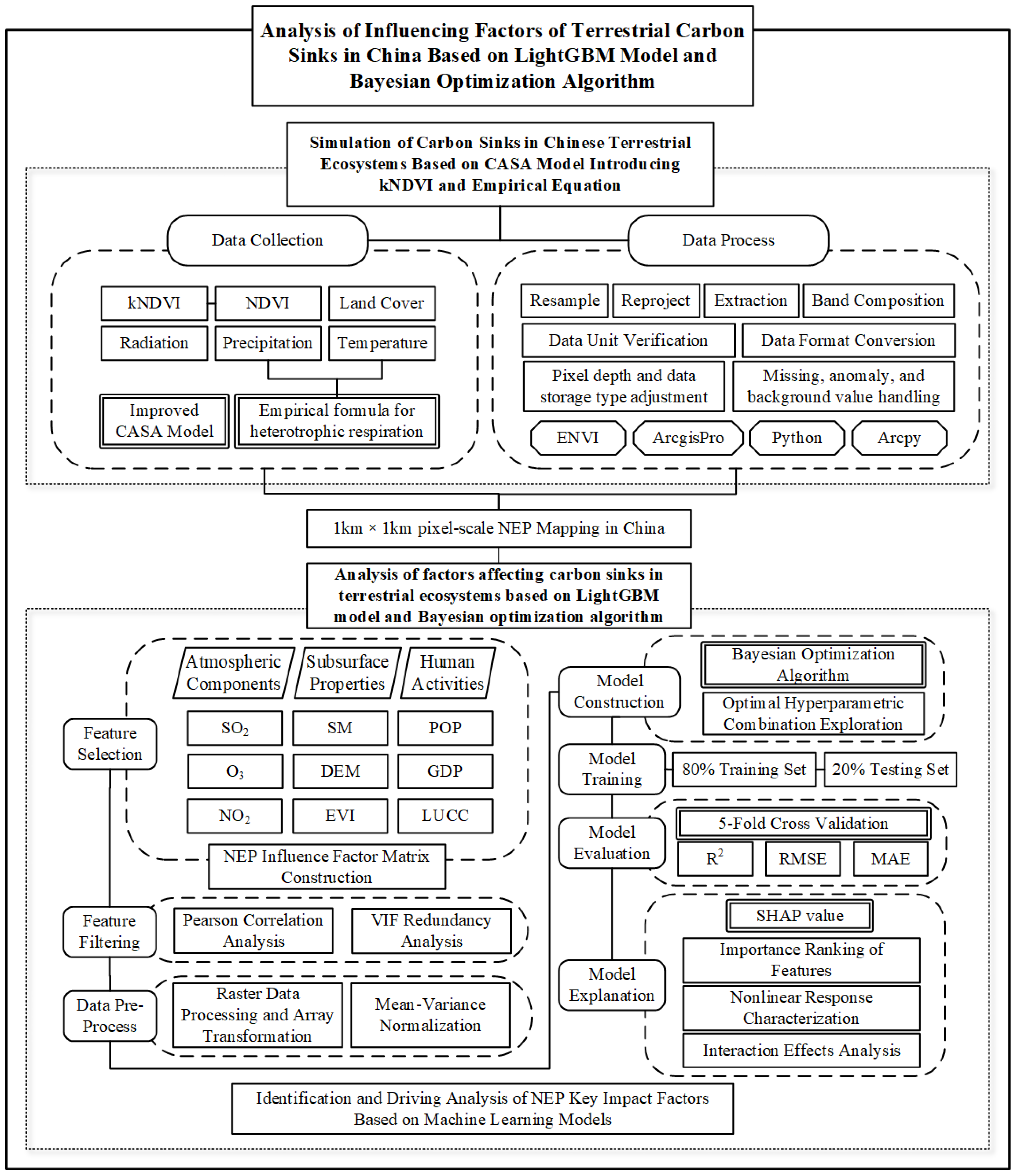
2.4. Methodological Framework

Figure 3 shows the workflow of this study.

3. Results

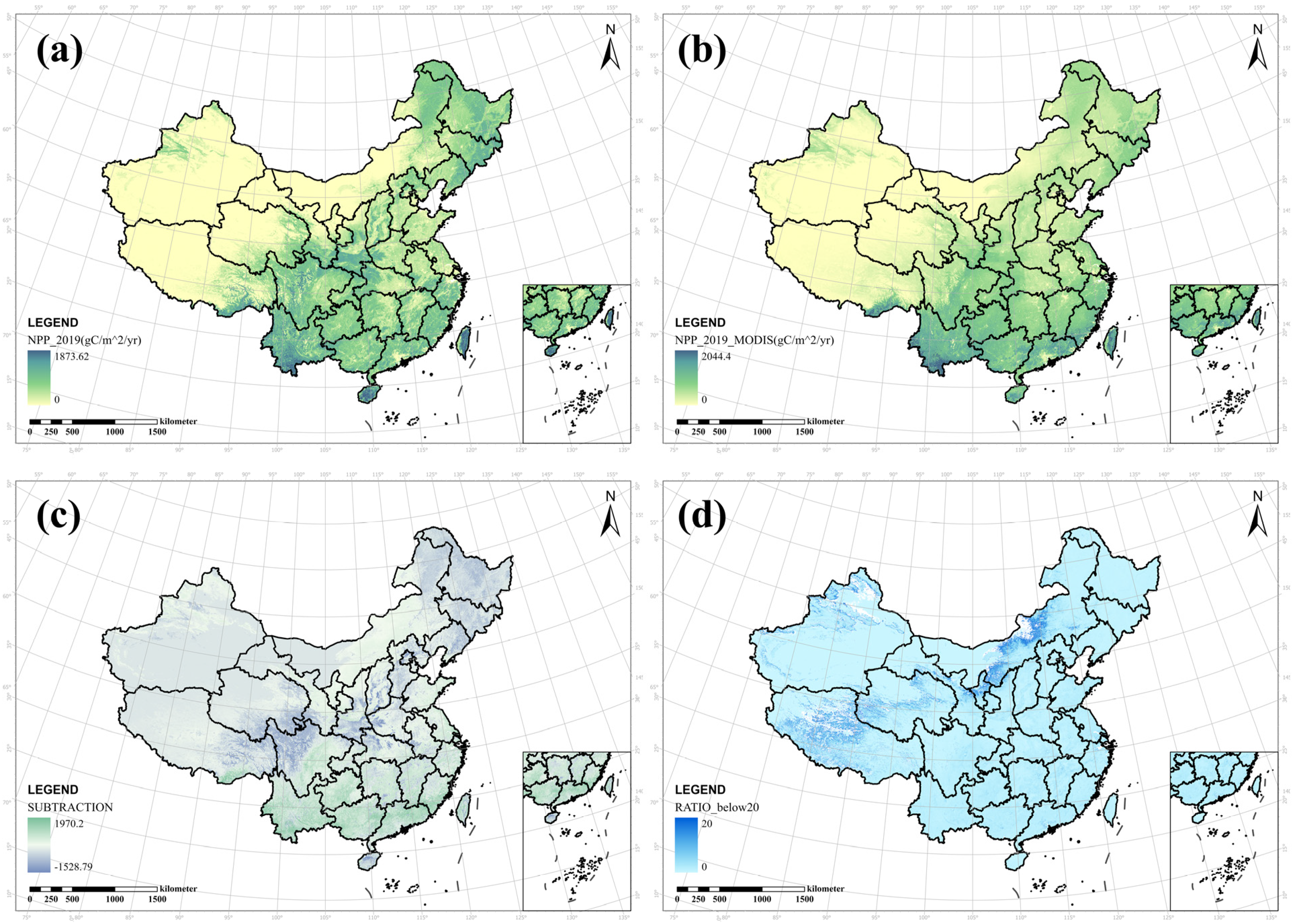
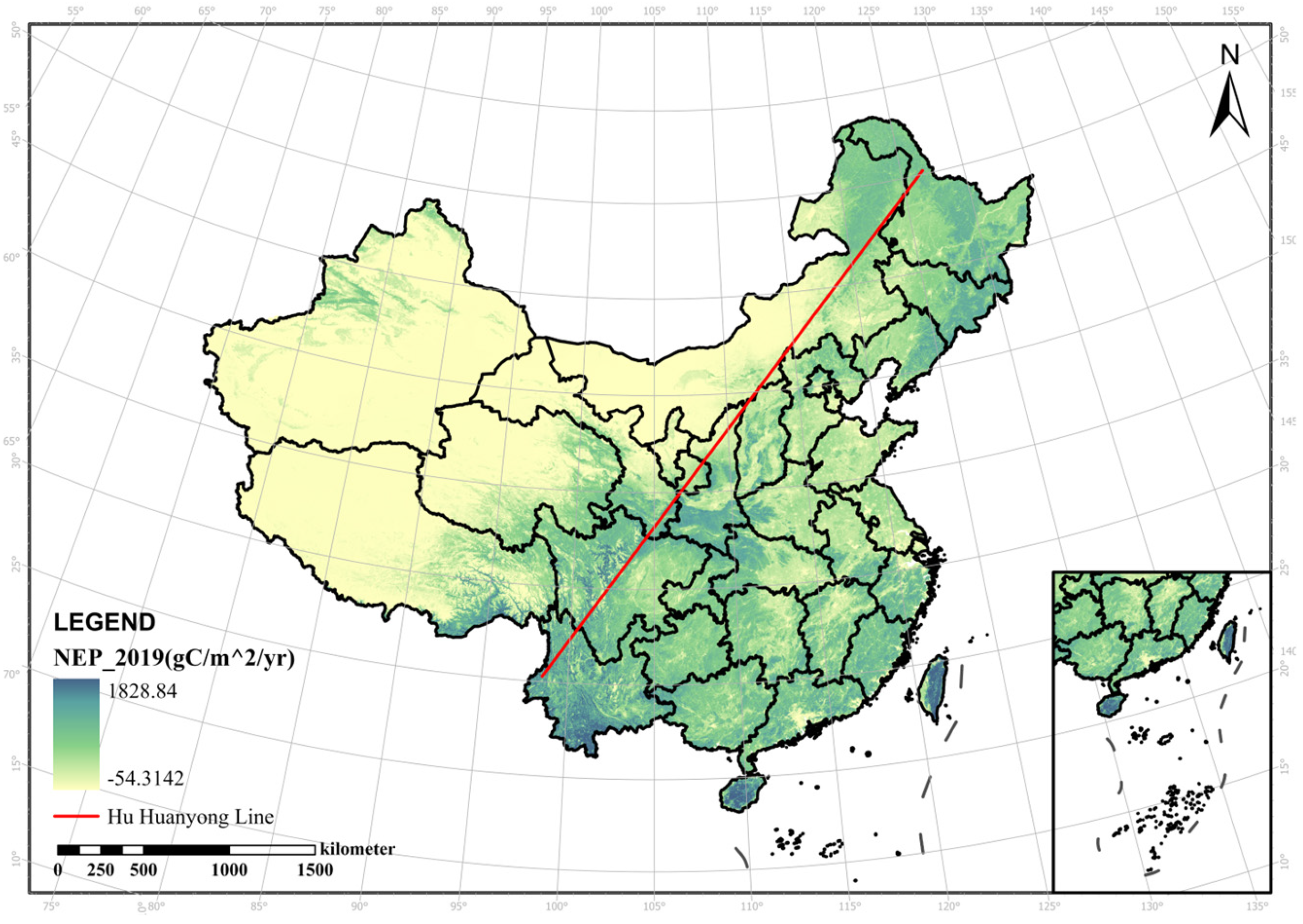
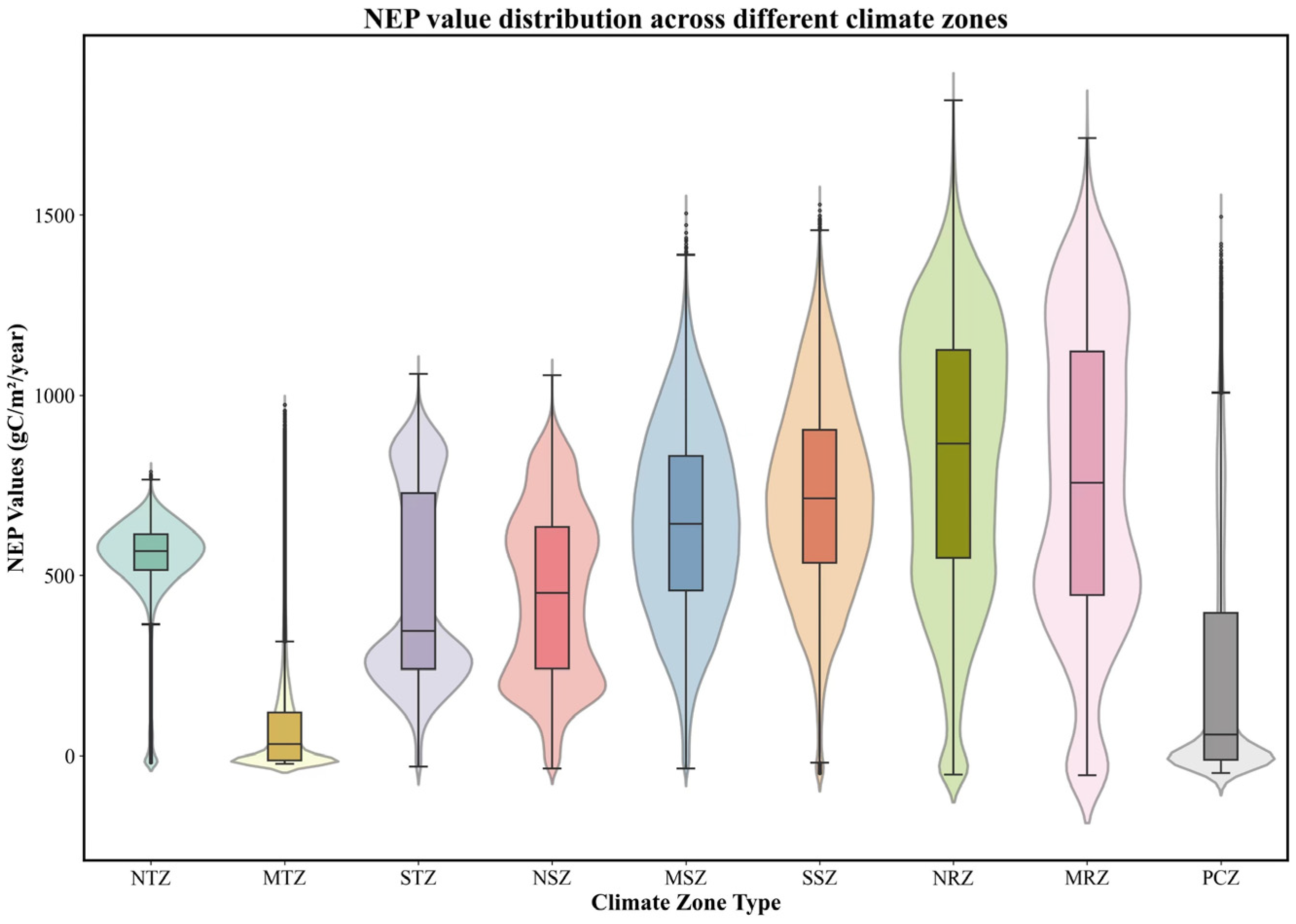
3.1. NEP Simulation and Analysis

The pixel-by-pixel calculation of NEP was conducted through the kNDVI-introduced CASA model and R_h equation in this study, and the results showed that the average of NEP at the pixel-scale and in China was 268.588 gC/m²/yr, with the sum of 2.541 PgC/yr in the whole region. To assess the reliability of our results, Pearson test was conducted between our results and the MOD17A3 NPP product, and the result is 0.832, showing a high correlation. We also compared the spatialization difference between them, which is provided in Figure A1. Compared with our research, it was found that our NEP result is similar to the ones derived by studies [16,63] also using the CASA methods, and support from inventory data was provided in such research. For the validation of the R_h methodology used in this study, it has also been supported by several studies [64,65]. Therefore, we think that our simulation result can be used in the further analysis.

Figure 4 shows the spatial distribution of the NEP pixel-level values in China in 2019. Analyzed from the perspective of administrative divisions, NEP values in the south of the Hu Huanyong Line are obviously higher than those in the north part. In addition, the eastern part in the Qinghai Province, the southeastern part of the Tibet Autonomous Region, and the northeastern corner of the Inner Mongolia Autonomous Region show relatively obvious high values of carbon sinks within their provincial boundaries. An obvious high value with mountainous distribution can be observed in western Sichuan and southern Tibet, and the Fujian Province, Taiwan Province, Hainan Province, and Yunnan Province show a relatively uniform high-value distribution. On the contrary, the northwest region is in the overall state of the carbon source. In addition, the model simulation results of this study can also reveal the negative impact of urbanization on terrestrial carbon sinks to a certain extent: economically developed areas such as Southern Jiangsu, Shanghai, and Northern Zhejiang in the Yangtze River Delta (YRD) region reflect a lower distribution of values, and in Guangdong Province, a clear distribution of low values can be observed in the central region, which is coincident with the distributional status of the Pearl River Delta (PRD) region.

After conducting the function of zonal statistics in ArcgisPro 3.0.2, Figure 5 shows that each climate zone embodies significant NEP distribution heterogeneity within and between groups. It can be observed that NRZ shows the highest average NEP value at the pixel-scale, which is 828.631 gC/m²/yr; the PCZ and MTZ are the two subzones with the lowest NEP levels, 134.812 gC/m²/yr and 205.963 gC/m²/yr, respectively. An obvious bimodal distribution can be observed in STZ, NSZ, NRZ, and MRZ, which may indicate greater complexity and significant source variation and compositional aggregation in NEP composition. Meanwhile, MSZ and SSZ show more uniform and smooth NEP distribution characteristics, which points to a stable and healthy ecosystem carbon sink function in these zones. In addition, NTZ, MTZ, and PCZ have more obvious trailing phenomena, reflecting stronger anomalies in these regions. We also conducted a Tukey test to examine the difference between the climate zones, and the result can be found in

Table A1. Tukey test result for NEP in different climate zones.

Multiple Comparison of Means—Tukey HSD, FWER = 0.05
group1	group2	meandiff	p-adj	lower	upper	reject
NTZ	MTZ	529.6591	0	523.0064	536.3118	TRUE
NTZ	STZ	190.2974	0	183.9476	196.6473	TRUE
NTZ	NSZ	164.2991	0	157.937	170.6611	TRUE
NTZ	MSZ	398.6029	0	392.1926	405.0132	TRUE
NTZ	SSZ	504.3487	0	497.9808	510.7167	TRUE
NTZ	NRZ	596.4504	0	590.0097	602.8911	TRUE
NTZ	MRZ	813.1031	0	806.2442	819.962	TRUE
NTZ	PCZ	119.1706	0	112.8199	125.5213	TRUE
MTZ	STZ	−339.362	0	−341.454	−337.27	TRUE
MTZ	NSZ	−365.36	0	−367.489	−363.231	TRUE
MTZ	MSZ	−131.056	0	−133.325	−128.787	TRUE
MTZ	SSZ	−25.3104	0	−27.4566	−23.1641	TRUE
MTZ	NRZ	66.7913	0	64.4381	69.1445	TRUE
MTZ	MRZ	283.444	0	280.1124	286.7756	TRUE
MTZ	PCZ	−410.489	0	−412.583	−408.394	TRUE
STZ	NSZ	−25.9984	0	−26.7686	−25.2282	TRUE
STZ	MSZ	208.3055	0	207.2055	209.4054	TRUE
STZ	SSZ	314.0513	0	313.2336	314.8689	TRUE
STZ	NRZ	406.153	0	404.8881	407.4178	TRUE
STZ	MRZ	622.8057	0	620.1295	625.4819	TRUE
STZ	PCZ	−71.1268	0	−71.7969	−70.4568	TRUE
NSZ	MSZ	234.3038	0	233.1357	235.472	TRUE
NSZ	SSZ	340.0497	0	339.1423	340.957	TRUE
NSZ	NRZ	432.1513	0	430.8267	433.476	TRUE
NSZ	MRZ	648.8041	0	646.0991	651.509	TRUE
NSZ	PCZ	−45.1284	0	−45.9055	−44.3514	TRUE
MSZ	SSZ	105.7458	0	104.5459	106.9458	TRUE
MSZ	NRZ	197.8475	0	196.3076	199.3874	TRUE
MSZ	MRZ	414.5002	0	411.6836	417.3168	TRUE
MSZ	PCZ	−279.432	0	−280.537	−278.328	TRUE
SSZ	NRZ	92.1017	0	90.7489	93.4544	TRUE
SSZ	MRZ	308.7544	0	306.0356	311.4732	TRUE
SSZ	PCZ	−385.178	0	−386.002	−384.354	TRUE
NRZ	MRZ	216.6527	0	213.7677	219.5378	TRUE
NRZ	PCZ	−477.28	0	−478.549	−476.011	TRUE
MRZ	PCZ	−693.933	0	−696.611	−691.254	TRUE

. The Tukey HSD test result confirms that NEP varies significantly among climate zones.

3.2. Preprocessing LightGBM Model Construction

3.2.1. Factor Choosing

For the analysis of the influencing factors, variables were selected from the levels of atmospheric components, subsurface properties, and human activities: the sulfur dioxide (SO₂), nitrogen dioxide (NO₂), ozone (O₃), soil moisture (SM), enhanced vegetation index (EVI), digital elevation model (DEM), population data (POP), gross domestic product (GDP), and land use and land cover change (LUCC). The mechanism of the effect of each factor on NEP is organized in

Table 3. Influencing mechanism between factors and NEP.

Influencing Aspects	Factor	Influencing Mechanism with NEP
Subsurface properties	SM	Soil moisture is one of the key factors affecting the growth of vegetation. At the same time, it can comprehensively feedback the influence of meteorological environmental conditions like water–heat balance. The vegetation will grow vigorously with suitable SM, while both the photosynthesis efficiency and the diversity of species in the ecosystem reach a high level, resulting a stable ecosystem structure. Based on that, plants can perform the function of carbon sinks better. On the contrary, vegetation growth will be limited due to exposure to water stress, then stomata will be closed, which in turn affects photosynthesis, respiration, and, consequently, the dysfunction of the carbon uptake.
	EVI	EVI is a commonly used index used to quantify and analyze the growth status and health of vegetation in the remote sensing field. It is calculated by combining the reflectance data of NIR, Red, and Blue bands. Due to the introduction of blue band, it can better resist the influence of atmospheric scattering and soil background and shows great sensitivity to detect the vegetation cover change. Furthermore, it can assess the health and stability of ecosystems.
	DEM	DEM is a kind of ground elevation data commonly used in terrain analysis, which can reflect the spatial characteristics and pattern of vegetation distribution as a sign related to the plant growth condition.
Atmosphere components	SO2	Sulfur dioxide is chemically active and easily interacts with other atmospheric components, causing acid rain and affecting plant growth. Sulfate aerosols are easily generated after meteorological oxidation and other processes, which may have impact on terrestrial carbon sink through the cooling effect and diffusion–radiation fertilization effect.
	NO2	Nitrogen dioxide was chosen as a major indicator for nitrogen deposition. Within a certain amount of nitrogen deposition, it is conducive for plant photosynthesis and growth, while excessive nitrogen deposition may lead to an imbalance in the proportion of plant nutrient elements, thus changing the morphology and structure of the plant and increasing its sensitivity to natural stresses. Other issues like affected micro-organisms’ activity and soil acidification will be triggered under the same circumstances.
	O3	Except for the well-known properties of air pollutants, ozone is a type of greenhouse gas with interactive effects in the atmosphere, climate, and ecosystem. Ozone formation originates from the oxidation process of oxygen atoms decomposed by ultraviolet radiation in the stratosphere. It also shows warming effect on atmospheric temperatures in the troposphere. In addition, increased concentrations of carbon dioxide contribute to global warming, which in turn may affect the rate of chemical reactions in the atmosphere and the production of ozone.
Human activity	LUCC	LUCC directly represents structural changes of the terrestrial ecosystem from human activities.
	POP	POP embodies the pressure of human activities on the ecosystem from the acceptance level.
	GDP	GDP, as the core economic indicator of the society system, indirectly reflects the intensity of anthropogenic life and production. Moreover, mutual compromises and trade-offs between financial benefits and environmental protection implements should be considered when conducting economic activities.

.

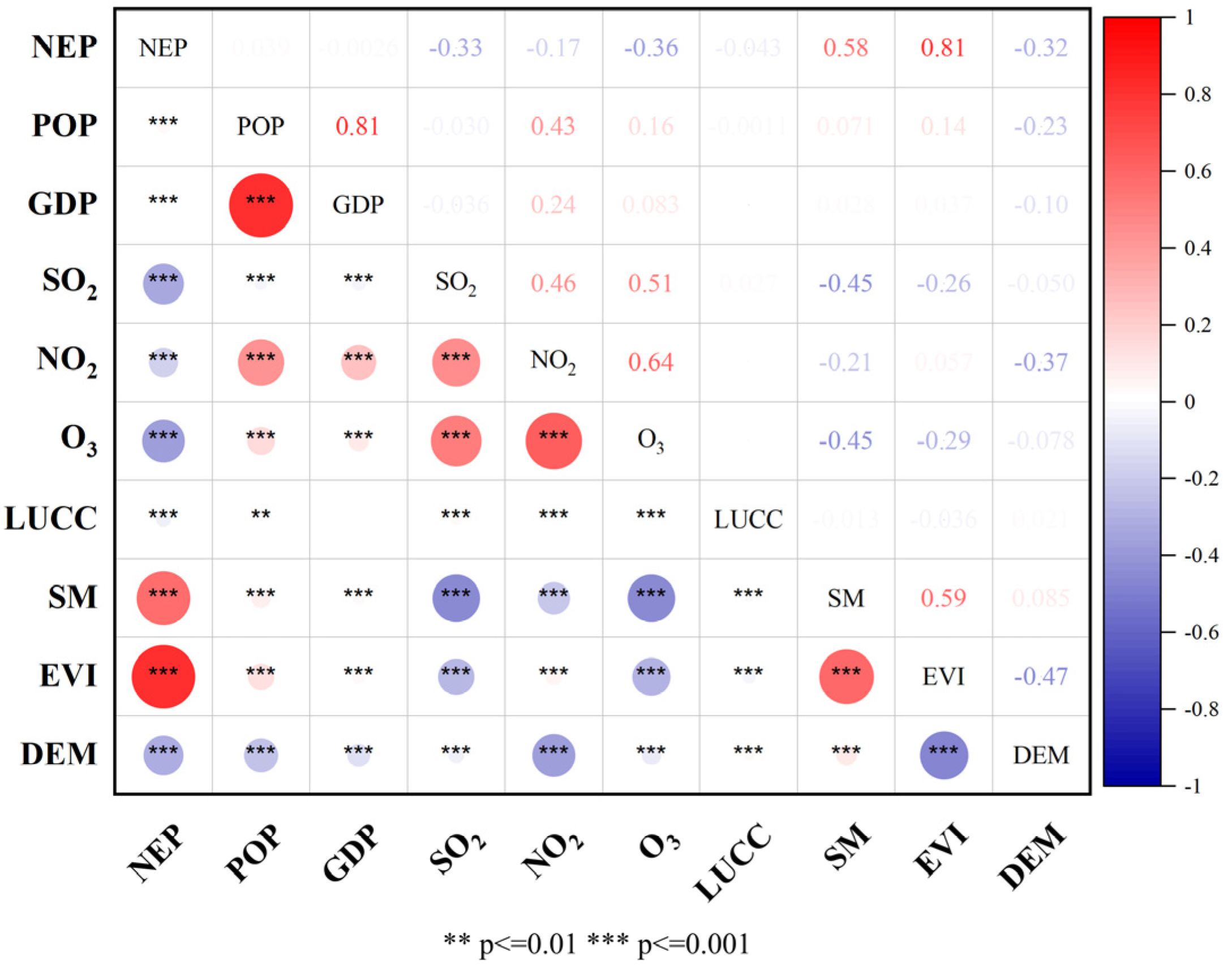
3.2.2. Factor Pre-Test

The preliminary analysis of the covariance check of the input data was performed using the Pearson correlation coefficient (Figure 6). Although the LightGBM model reflects a more inclusive distribution of the model input data, it would be more beneficial to the robustness of the model if the multiple covariance checks can be performed beforehand. If the correlation coefficient value is higher than 0.85, then the factor will be considered for removal in conjunction with the actual contribution. Figure 6 shows the results of the correlation analysis between the variables selected in this study.

To be mentioned, mean-variance normalization was applied to the features as the input for the LightGBM model, scaling all the variables into distributions with a mean of zero and a variance of one. The aim is to adjust the data scales of variables with different magnitudes and units to ensure that they have the same impact in the model training and, at the same time, the training speed can be lifted. It is suitable for features with no obvious boundaries in the data distribution and the possibility of having extreme features. The Pearson test was applied to the normalized data and it can be seen that each factor after normalization does not exceed the exclusion threshold of 0.85, which means that it can be retained for the subsequent modeling work as the initial judgment.

The multicollinearity of the selected variables was further tested using variance-inflated factor analysis [66]. Factors which appeared above a threshold of 10 would be eliminated before LightGBM model training. The VIF test result (

Table 4. VIF test result for each influence factor.

	Variable	VIF
0	const	204.0833
1	POP	3.8633
2	GDP	3.1652
3	SO2	1.6768
4	NO2	2.7715
5	O3	2.2426
6	LUCC	1.0023
7	SM	2.4383
8	EVI	2.6518
9	DEM	1.9366

) showed that only the constant term had a very high value of the VIF (204.0833), which is normal in the VIF calculation for it does not show variance. The rest of the influencing factors’ VIF values are much less than 10, which are within the normal range, indicating that there is no serious problem of multicollinearity between these variables and all variables can be retained into the machine learning regression model as the input.

3.2.3. Factor Process

Based on the representativeness and diversity of the indicators as well as the authenticity and availability of the data, the selection of each impact factor and NEP was chosen in 2019 out of consideration for the completeness of the data collection. To be mentioned, the LUCC data in this study were extracted with the land expansion analysis strategy (LEAS) part of the epatch-generating land use simulation (PLUS) model [67] using CLCD data from 2019 to 2020 to represent land expansion in 2019. The land cover types addressed in CLCD with coding one-to-nine are cropland, forest, shrub, grassland, water bodies, snow and ice, bare ground, impervious surfaces, and wetlands. Each category identifier in the PLUS results is the same as the original encoding system in CLCD, indicating that an exact change occurred in that category, while an extra zero category points to a situation where no land use change has occurred in that time period.

All the collected input raster data also need to be processed in the same way as the input for the CASA model to reach uniform spatial reference information, the spatial and temporal resolution, and data details with the NEP data output in the previous section. The values of each raster piece of data were then extracted to the image center by converting to point elements; therefore, a total of 9,459,982 sample point data were obtained as the model input for machine learning.

Table 5. Statistical indicators of the initial distribution of the input variables.

	Count	Mean	std	min	0.25	0.5	0.75	max
NEP	9,459,982	268.588	293.804	−54.314	−10.905	199.914	484.279	1828.840
POP	9,459,982	149.391	529.074	0	2	20	147	54,388
GDP	9,459,982	1064.058	8958.257	0	9	74	531	3,100,009
SO2	9,459,982	11.561	2.452	2.700	9.900	11.500	13.100	44.700
NO2	9,459,982	17.220	6.222	4.800	13.400	15.200	18.400	63.200
O3	9,459,982	98.150	10.165	59.800	91.500	97.700	104.800	134.200
LUCC	9,459,982	0.036	0.433	0	0	0	0	9
SM	9,459,982	287.039	105.634	35.115	216.836	301.395	365.227	599.260
EVI	9,459,982	0.395	0.251	−0.087	0.126	0.446	0.614	1.000
DEM	9,459,982	1835.057	1740.314	−268	431	1162	3191	8405

offers the statistical metrics of the input variables with the original distribution.

3.3. LightGBM Modeling with Bayesian Optimization

3.3.1. Model Construction

Based on the LightGBM algorithm, this study chose NEP as the response variable and the chosen nine influencing factors as the characterization variables to fit the regression task. The division ratio of the training set and the testing set was 80% and 20%, respectively. The five-fold cross-validation method was used to test the model training validity at the same time as Bayesian optimization was applied to explore the optimal hyper-parameter combinations for the model construction. The coefficient of determination (R²), root-mean-square error (RMSE), and mean absolute error (MAE) were selected as the evaluation metrics of the model performance. After combining several rounds of iterations of the Bayesian optimization algorithm, the final values of the hyperparameters of the LightGBM model constructed in this study are as follows: {num_leaves: 134, learning_rate: 0.05, feature_fraction: 0.88, bagging_fraction: 0.85, bagging_freq: 5, min_gain_to_split: 0.01, max_depth: 5, min_child_samples: 28, reg_alpha: 4.9, reg_lambda:5.65, num_boost_round: 860}.

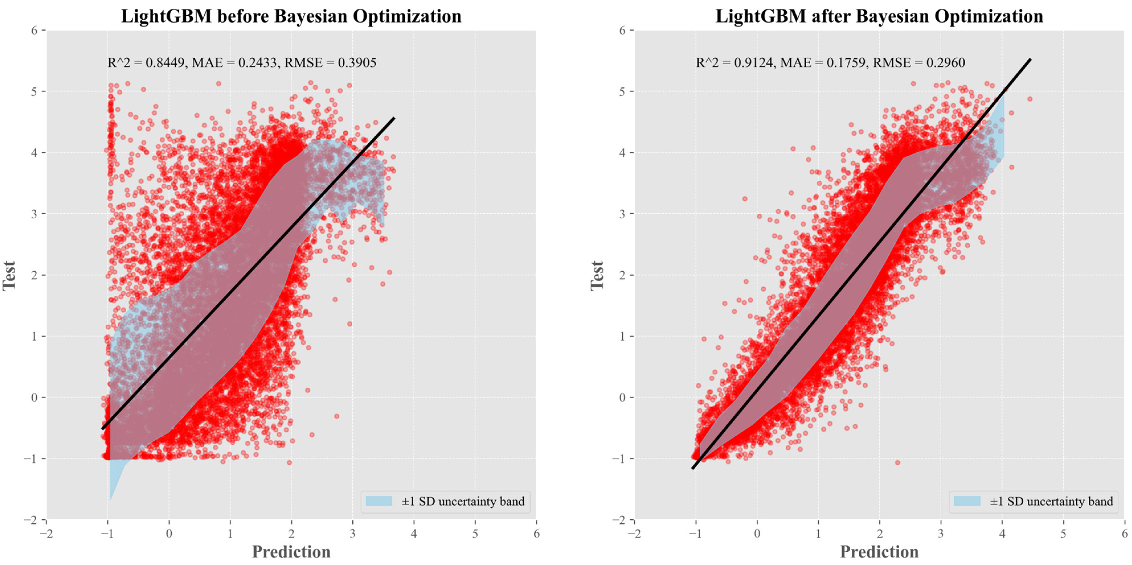
3.3.2. Model Evaluation

Table 6. Five-fold cross-validation results of LightGBM model constructed in this study.

	RMSE (gC/m2/yr)	MAE (gC/m2/yr)	R2
Fold1	0.2961	0.1761	0.9124
Fold2	0.2960	0.1758	0.9125
Fold3	0.2958	0.1757	0.9124
Fold4	0.2955	0.1757	0.9126
Fold5	0.2965	0.1762	0.9121
mean	0.2960	0.1759	0.9124

indicated that the LightGBM model constructed in this study showed a high simulation performance, and the combination of Bayesian optimized hyperparameters significantly improves the explanation of the model (Figure 7). R² improved from 0.8476 to 0.9124, while the MAE and RMSE decreased by 27.73% and 24.20%, respectively, demonstrating the superior enhancement for the model construction.

To analyze the model uncertainty, we added ±1 standard deviation (SD) bands around the predicted values. The bands were computed by first binning the predicted values, calculating the mean and standard deviation of the residuals in each bin, and then constructing the upper and lower bounds. These bands reflect how the spread of errors varies with the prediction magnitude and help evaluate the model’s consistency and heteroscedasticity. By comparing the two subplots in Figure 7, it can be observed that after Bayesian optimization, the uncertainty bands became significantly narrower, suggesting that the model’s predictions became more stable and concentrated. This improvement is also consistent with the observed enhancement in the predictive performance metrics. The reduced spread of residuals suggests that the optimized model generalizes better and exhibits more reliable behavior when applied to unseen data.

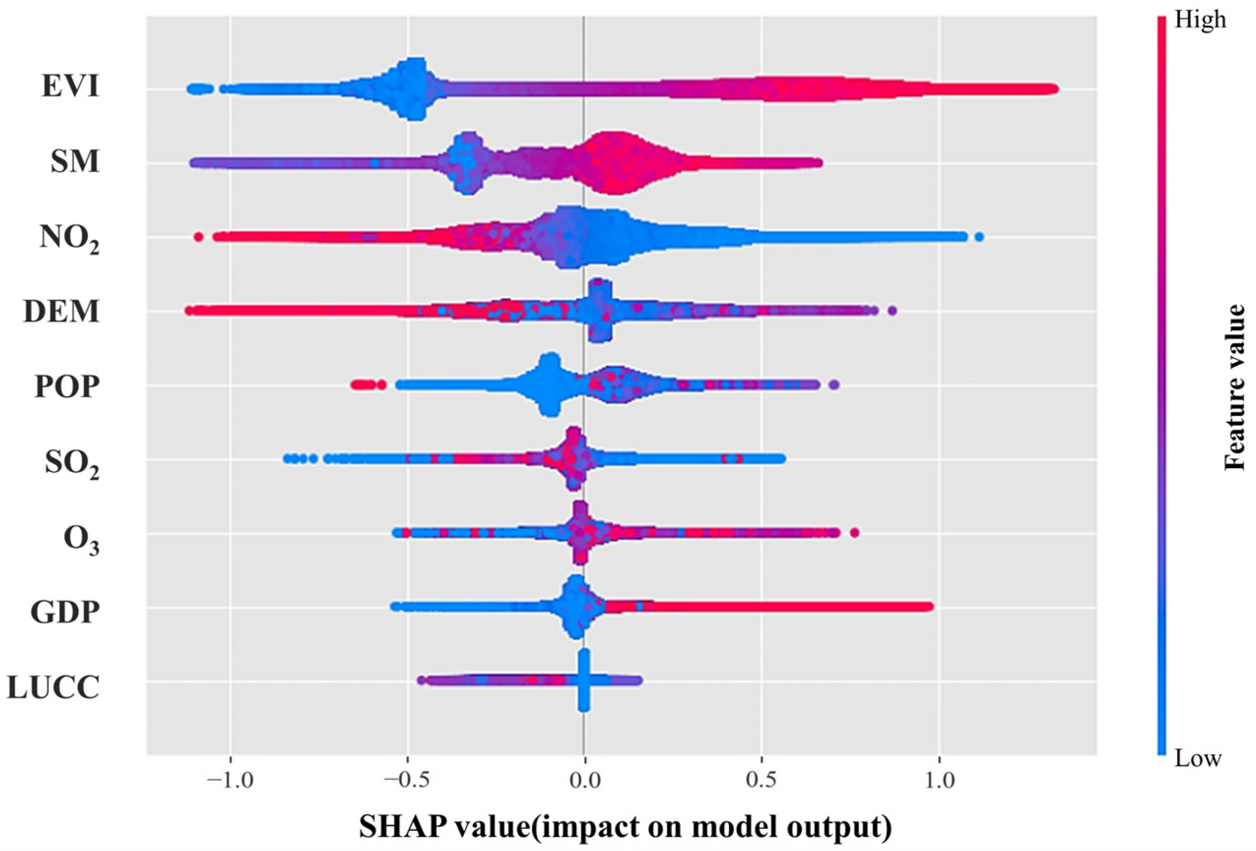
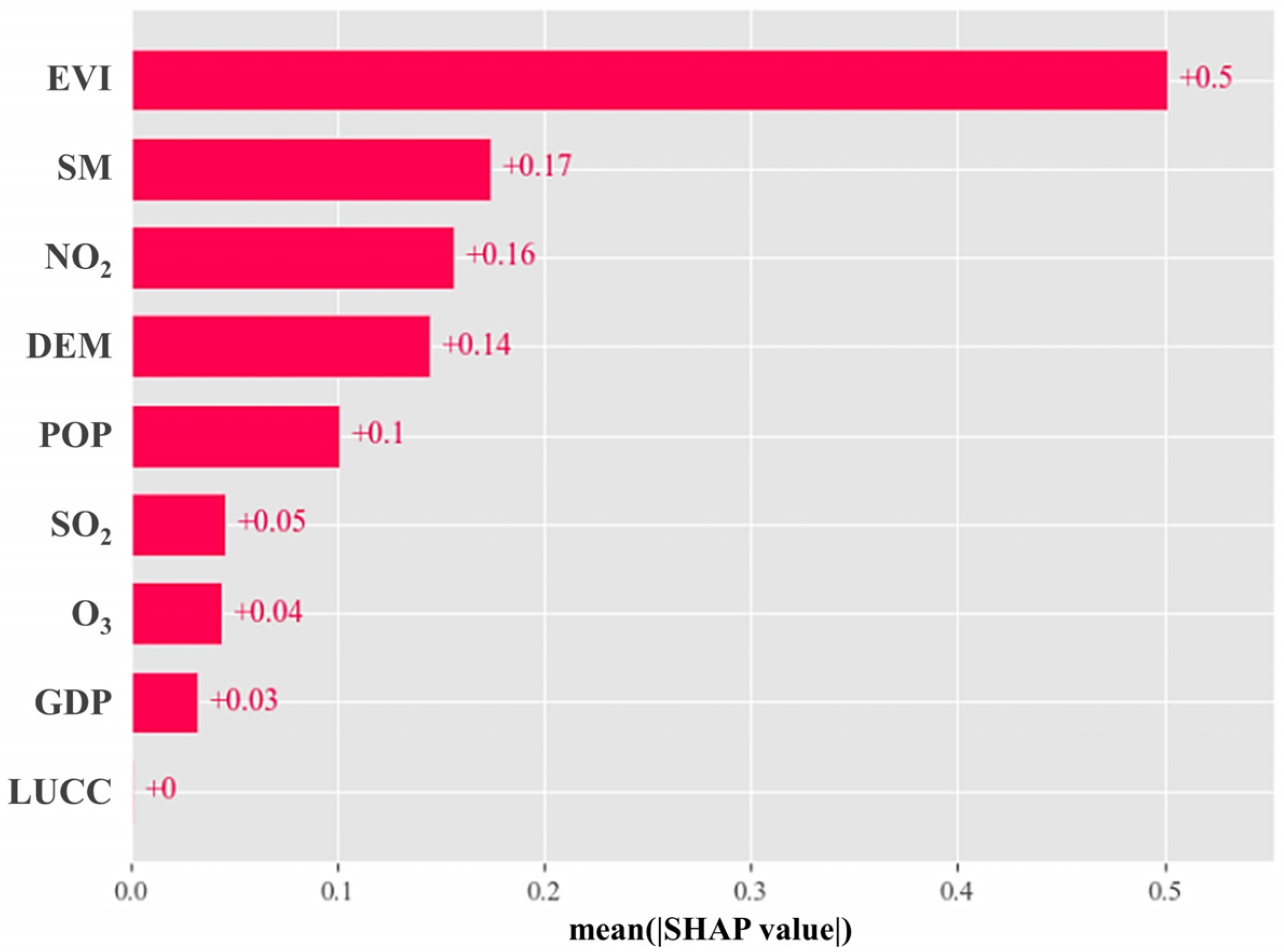
3.4. Model Explanation Base on SHAP Value

3.4.1. NEP Drivers’ Contribution Ranking

The SHAP swarm plot (Figure 8) was applied to illustrate the relative magnitude and direction of the influence and the distribution and density of the selected factors on NEP. The left and right ends of the horizontal axis correspond to the negative and positive influences on the model, and the closer the ends are, the greater the influence of the feature on the model output. Meanwhile, the color mapping shows the value distribution of the data themselves; the closer to the red color means that the feature is at a higher value and the closer to the blue color means the lower value. Specific evolutionary details for each variable will be analyzed in conjunction with the dependency plots in the next sections, and the generalizations are mainly illustrated in this part.

Among the factors who have a trend of high values corresponding to positive model impacts and low values pointing to negative model impacts, the widest range of action is reflected in the EVI and SM, then in O₃ and GDP as well. On the contrary, the exact opposite trend can be observed in NO₂ and DEM. In particular, with respect to the aggregation, SM reflects one positive and one negative SHAP value cluster simultaneously. POP shows a clearer segregation of characteristics in the negative SHAP. For the aggregation characteristics of the EVI and POP, a low feature value together with negative SHAP values can be observed, while for NO₂ and DEM, the aggregation characteristics of a low eigenvalue aligned with positive SHAP are more predominantly reflected. The aggregation of the remaining factors is approximately distributed around the SHAP = 0 value.

Both Figure 8 and Figure 9 revealed that the EVI from the dimension of subsurface properties was the most critical variable affecting terrestrial carbon sinks, with the absolute SHAP value of 0.5. Meanwhile, SM, NO₂, and DEM show similar proportions with the contribution from 0.14 to 0.17, belonging to the dimensions of subsurface properties and atmospheric components. This further illustrates the importance of subsurface properties for terrestrial carbon sinks, and the importance of NO₂, which is used to characterize the fraction of nitrogen deposition, was emphasized with the highest impact on NEP as an atmospheric component. The other rest two atmospheric variables chosen were close to each other for the importance level. Analyzing from the perspective of human activities, POP achieves the highest importance (|SHAP| = 0.1), ranking in the middle considering the contribution in the model constructed in this study.

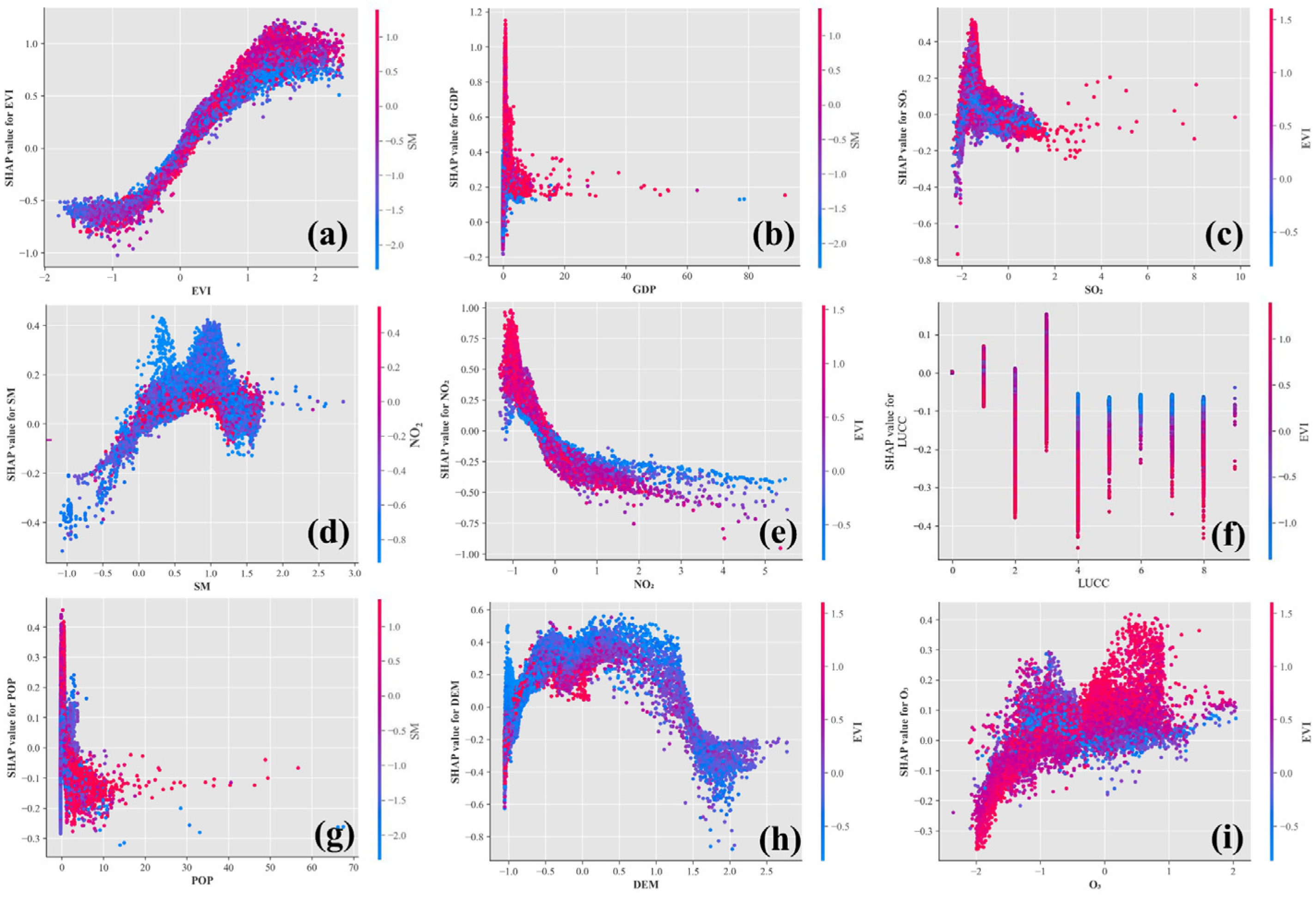
3.4.2. Nonlinear Response Analysis of NEP to Driving Factors

Based on the feature importance analysis, the inter-relationships between NEP and the nine drivers are further grounded using dependency plots. Dependency graphs characterize the evolution of the impact of each influential factor on the contribution of the model, taking into account the interactions with the other factors. The horizontal axis of the image represents the range of factor values, representing the magnitude of the feature value in each sample. The vertical axis represents the SHAP value of the factor in the model trained in this study, indicating the contribution to the model prediction results. A positive SHAP value means that the factor has a positive effect on the prediction result in that sample, which will increase the output of the model prediction; a negative SHAP value means that its contribution is negative, which will decrease the model prediction. Observing the scatter distribution in Figure 8, it can be seen that the LightGBM model captures the nonlinear relationship between the factors and the model response well. It is important to propose that all the factors mentioned in the analysis for Figure 10 are normalized ones.

(1)

EVI

As shown in Figure 10a, a clear positive effect can be observed in the distribution pattern of the SHAP values of the EVI: as the value of the EVI increases, the higher its SHAP value is, the greater the positive effect on the model, while echoing the corresponding analysis in the swarm plot in the previous section.

(2)

SM

For the contribution curve of SM to the model (Figure 10d), a more pronounced trend of a nonlinear response is shown, and a clear upward and then downward undulating trend can be observed for its SHAP curve. Two peaks of its SHAP value appeared at positions corresponding to SM = 0.25 vs. 1. Negative values of SM reflect a negative influence on the model prediction, and then the contribution to the model gradually turns positive as the SM expands. When the SM exceeds 1, its SHAP value will reflect a decreasing trend again, and can even turn into a negative influence. This indicates that the positive influence of SM on NEP should also occur in a reasonable value range, and either too high or too low will have an inhibitory effect on NEP.

(3)

NO₂

In the model constructed in this study, NO₂ embodied a significant negative impact on the model prediction performance (Figure 10e). As the value of NO₂ increases, its SHAP gradually shows an accurate decreasing trend.

(4)

DEM

The dependence plot of the DEM (Figure 10h) reflects a clear inverted U-shaped distribution. Firstly, the SHAP value in the lowest value band of DEM shows a rapid increasing trend, and after the normalized DEM reaches about −0.5, the SHAP value shows a flat high-value state and is distributed in the positive value region, indicating that the DEM reflects a positive modeling effect in the interval of [−0.5, 1.25]. Then as the DEM value increases, its SHAP value gradually decreases, and the trough of the SHAP value appears near DEM = 2. Afterwards as the DEM rises, its SHAP value slightly recovers and presents a negative value state. Thus, an appropriate range of DEM values will have a stable positive impact on the model prediction. Beyond a certain threshold, its SHAP began to decline with the increase in the DEM, and in the highest value of the interval reflects a slight rebound finally.

(5)

SO₂

By observing the distribution of points in Figure 10c to analyze the trend of SO₂ with its SHAP value, it can be seen that the SHAP value of SO₂ shows an increasing and then decreasing trend with the gradual increase in the SO₂ value. Its SHAP value obtains a positive peak of more than 0.4 at SO₂ of −1.85.

(6)

O₃

The response pattern of O₃ with its SHAP in general shows a tendency to rise with increasing O₃ values, and it might be clearer to analyze in combination with its interactive relationship with the EVI (Figure 10i).

(7)

GDP and POP

The two factors, POP (Figure 10g) and GDP (Figure 10b), reflect similar but slightly different SHAP plot distribution characteristics. The lowest values of both GDP and POP affect NEP to the largest extent, while as the values of the two variables increase, GDP embodies a slightly delimited distribution at a SHAP value of 0.2 and has a positive effect on NEP to some extent. And as POP increases, the distribution of negative SHAP points can be observed, and the scatter radiation range of POP is larger than that of GDP, indicating that POP is more likely to influence NEP. So, in the model constructed in this study, the appropriate GDP corresponding to the decent intensity of economic activities can promote the increase in terrestrial ecosystem NEP to a certain extent, while POP mainly embodies the negative effect on NEP, and with its increase, this negative effect will be gradually reduced.

(8)

LUCC

Figure 10f illustrates that Types 2 and 3 positively influence model predictions, corresponding to land expansion categories of forest ecosystems and shrub ecosystems. Category 0, which corresponds to pixels that did not undergo a land-use type shift, shows a SHAP value of 0, which is consistent with the perception. While category 1, which is associated with a shift to the cropland land category, shows a slightly wider SHAP distribution than category 0. The remaining categories all show negative SHAP values.

3.4.3. Interactive Relationship Characterization Between Variables

Dependency graphs will also provide information about the interactions between the input variables. SHAP will select features based on the principle of maximum relevance and reflect the interaction between features with the color map. Thus, the factor on the right side in Figure 10 is the variable that the model automatically calculates and determines to have the strongest interaction with the selected influential feature, and the color-coded mapping corresponds to the range of values for the interactive factor. The closer to red represents a high value for the factor, while the closer to blue indicates that the factor value is low in this sample. Observing whether there is a pattern in the color distribution can provide a basis for interpreting the interaction between factors.

(1)

EVI: interaction with SM

For the interaction effect between the EVI and SM, a clear stratified distribution can be observed as well in Figure 10a. As the EVI rises, the SHAP values of sample points with higher SM values have a larger radial range in both positive and negative data. While for sample points with low and medium SM values, the slopes of the rising curves are gentler and the effects on the model are relatively smaller. It suggests that high values of SM are more likely to interact with the EVI and amplify the positive effects of the EVI on model predictions.

(2)

SM: interaction with NO₂

For the interaction effect between the SM and NO₂ (Figure 10d), a large area of blue scattering can be observed in particular, indicating that low values of NO₂ are more likely to interact with the SM. With the increase in the SM, its interaction of low NO₂ has an increasing, then decreasing effect on NEP, changing from negative to positive. In other words, low levels of NO₂ and low levels of SM can greatly affect NEP negatively, and the red color of high values of NO₂ in the interval (0, 1.5) is more concentrated in the positive region of a SHAP value less than 0.25, which indicates that the combination of high values of NO₂ and appropriate levels of SM can have a positive effect on NEP.

(3)

NO₂: interaction with the EVI

For the interaction between NO₂ and the EVI, a clear stratified distribution feature can be observed in Figure 10e. The blue scatter corresponds to the low value of the EVI, which shows a gentler action curve, and the red–purple curve has a larger distribution range and slope, indicating that the high value of the EVI amplifies the effect of NO₂ on NEP. And in the positive region of this image SHAP, the EVI is mainly concentrated in the region of its high value, indicating that for the sample points with high EVI values, lower levels of NO₂ can produce higher contributions to the model here, suggesting that appropriate concentrations of NO₂ can be absorbed by some vegetation and converted into carbon sink storage. And with the increase in NO₂, the decrease in the EVI can minimize its negative impact on the model simulation.

(4)

DEM: interaction with the EVI

Talking about the interaction between the DEM and EVI, firstly, observing the color distribution pattern in Figure 10h, it is remarkable to observe a certain hierarchical feature overall that the blue scatters have the largest proportion, while the distribution of purple curves is immediately below the blue curves, and finally, a small portion of red scatters are distributed. Analyzing the value domain intervals of the two factors, it shows that the positive effect of the DEM on NEP decreases with the increase in the EVI in a certain DEM interval (from about −0.5 to 0). This suggests that lower elevations have a negative effect on the carbon sink capacity of healthier vegetation, possibly due to the mismatch between vegetation growth requirements and the hydrothermal conditions that the geography can provide.

(5)

SO₂: interaction with the EVI

For the interaction between SO₂ and the EVI, observing the pattern of color changes in Figure 10c, it is found that the scatters of different colors embody roughly the same distributional trend, indicating that the full-value range of the EVI and SO₂ show basically the same interaction characteristics. Meanwhile, it can be seen that the distribution range of blue scatters is more concentrated compared with that of the purple–red scatters, which suggests that the combination of medium and high values of the EVI and SO₂ can slightly amplify the positive effect on NEP. In addition, the red scatters occasionally appear in the high-value SO₂ region, proving that a high-value EVI is more prone to interaction effects.

(6)

O₃: interaction with the EVI

It can be observed that the red scatter has a certain distribution trend, showing a clear upward trend in the SHAP value of O₃ in the presence of high EVI values, indicating that the interaction between high values of the EVI and O₃ values tends to produce a positive model contribution. What is more, the model has the largest magnitude of both positive and negative effects at this time. For the blue–purple medium and low values of the EVI, the SHAP curve of O₃ tends to show a nonlinear wave-shaped distribution. In addition, the peak SHAP of medium and low EVI values is smaller than that of high EVI values combined with O₃. This indicates that the interaction between the EVI and O₃ is significantly different with the stratification of the EVI values, and high EVI values can promote the positive effect of O₃ on NEP relative to the medium and low EVI values.

(7)

GDP and POP: interaction with SM

Both GDP and POP showed the largest interaction effects with SM (Figure 10b,g), which had similar but slightly different color distribution patterns. The blue scatters corresponding to low SM values appeared more frequently in the low values of POP interval segments, indicating that at this time, the interaction between the appropriate soil moisture and POP can have a certain degree of effect on NEP. The reddish-purple scatters are distributed more widely both in the height of the Y-axis (corresponding to the effect on NEP) and the width of the X-axis (corresponding to the interval of values of the independent variables) in the two features, indicating that the middle and high SM values are more likely to interact with POP and GDP and have a greater effect on NEP. As for the interaction effect on GDP, the low-value SM scatters account for a rather small percentage of the distribution in the plot, indicating that lower soil moisture basically does not have an interaction effect with GDP.

(8)

LUCC: interaction with the EVI

In the analysis of the interaction effect between the EVI and LUCC (Figure 10f), the color mapping distribution is more completely represented in categories 4 to 8, corresponding to the transitions to the land classes of grass, water, snow, ice, bare ground, and impervious surfaces, which to some extent characterize the presence of vegetation degradation. The similar interaction pattern is observed for all conversion types: in all cases, with increasing EVI values, a decrease in the SHAP value of LUCC is observed at the corresponding sample point. Low EVI values reflect a milder negative impact on model predictions, suggesting that image points where LUCC conversion categories 4 to 8 occur tend to influence NEP more negatively with high EVI values. This conclusion actually is suitable for virtually every conversion type. Since the EVI is a reflection of vegetation health and growth in that sample, there is a positive correlation between pixels with high EVI values and their carbon sink values as concurrent photosynthetic products.

On the other hand, the occurrence of LUCC indicates a disturbance to the ecosystem and its surface cover, which will negatively affect NEP in the short term, regardless of whether it is a shift to the theoretical category of high-carbon-sink ecosystems or not. Meanwhile, the short time span corresponding to LUCC will strongly affect the identification result of image elements where the actual transformation occurs, and it will take a period of time for vegetation growth and emerging ecosystems to return to the steady state to develop and accumulate. So, the short time span selection may be unable to reflect the lagging effect of LUCC‘s impact on carbon sinks. In transition types 2 and 3, which correspond to forests and shrubs, the distribution of reddish-purple scattered dots is more concentrated, and the EVI relative to the median shows higher SHAP, which has a higher positive impact on the model prediction. In practical terms, areas with low EVI values may imply higher potential for carbon sink conversion, and appropriate management policies may be able to utilize the carbon sinks to a greater extent.

To summarize, the EVI is the largest interaction factor of the five factors (the LUCC, O₃, NO₂, SO₂, and DEM), followed by the SM, which corresponds to the strongest interaction characteristics of the three features (the EVI, GDP, and POP). Meanwhile, the largest interaction factor for SM was NO₂. The EVI mainly showed strong interactions with atmospheric components and subsurface properties, which is understandable because vegetation is the direct actor for atmospheric exchange, and the basal nature of the subsurface provides a solid support for vegetation growth, whereas SM is mainly a factor associated with human activities and a factor that characterizes the vegetation itself. The reason may lie in that human activities will affect the nature of the substrate including soil moisture, and it is reasonable for the SM as the combined effect of hydrothermal conditions to show the strongest correlation with the EVI.

3.4.4. The Influencing Effect Analysis for NEP Drivers

Our study points out the importance of subsurface properties on NEP, especially the effect of the EVI on carbon sinks. The positive correlation between a high EVI and high NEP is clearly captured. This consensus can be paralleled by the implements of reforestation and ecological restoration projects currently underway in China, aiming to improve the vegetation cover and healthy state. At the same time, the importance of SM is emphasized in our study, in terms of not only its contribution to NEP, but also its interaction with other factors, which is also pointed out by these studies [25,28,68] with the non-negligible importance of the SM to NEP. In practical term, SM is a factor that can be regulated in combination with management activities, and its marginal effect also needs to be considered. As shown in the Figure 10d, SM’s positive contribution to NEP will diminish when over a certain threshold. Therefore, for policy makers, irrigation operation as well as regular monitoring for soil should be fine-formulated in consideration with the ecosystem category and its water demand.

The inverted U-shaped action curve of DEM reveals the significance of site-specific planting policies; similar results can be found in Karimi et al. [69]. At the atmospheric component level, NO₂ shows the greatest NEP contribution, which might be echoed by studies emphasizing the importance of nitrogen deposition to NEP [11,70]. At the same time, distinct negative relationship curves and stratified interaction features are clearly observed. This points to the fact that the atmospheric control of combustion emissions from anthropogenic sources and industrial production could also be beneficial to the carbon sink function of natural ecosystems to a certain extent. The contribution of ozone to NEP seems, overall, positive but still complex, as well as its interaction characteristics, which might be in attribution to its high chemical activity and oxidation that makes it susceptible to environmental influences. Therefore, its relationship with NEP could be further explored with elaborately designed experiments. The distribution range of SO₂’s contribution to NEP is smaller than other factors, which may be due to the fact that SO₂ has a smaller distribution range than the other factors.

In addition, the contribution of human activities to NEP is, overall, poorer than expected. Firstly, analyzing from the aspect of factor, the interpretability of the LUCC is probably limited to the number of pixels extracted, while GDP and POP actually belong to the socio-economic data, which are more relevant and commonly used in carbon emission studies. On the other hand, the effects of human activities may be more apparently-revealed on the embodiment of the induced change towards carbon sinks, such as quantifying how much carbon sinks in the protected areas have been increased after ecological projects, or how much carbon sink loss happened in the built-up areas due to the urbanization process. The EVI and SM are found as the most likely to have an interactive relationship with other factors, which is a good sign because human management activities can be well engaged with these two factors. Meanwhile, in this study, the interaction mainly relies on observing whether the distribution of different colors could form a regular curve, observing the color stratification and aggregation. It provides a visualized insight from the perspective of the factor value domain, but may still have some difficulties in obtaining summative conclusions. To address this issue, analytical methods such as a geo-detector [23,71] that provide results on the type of interactions can be considered as a complement.

4. Discussion

4.1. Limitations of Carbon Sink Modeling

In terms of NEP simulation, the problem of a CASA model is that it does not have the relevant data considering human activities and management behaviors as other process models do. As a result, the NPP value it expressed is closer to the ideal and natural state without perturbation. In order to more realistically respond to the carbon sink of terrestrial ecosystems, it would be better to quantify and deduct the data of inference and human activities. For example, introducing the indicator of the anthropogenic activity intensity for refinement in each land cover type could be a trial. More specialized and advanced optimization algorithms [72] like Non-dominated Sorting Genetic Algorithm II (NSGA-II), Particle Swarm Optimization (PSO), and Ant Colony Optimization (ACO) can be considered in combination with the CASA model. If the data for human management or interference characterization are available, then the comparison of the difference between the nature reserve and human activities-influenced region [73,74] or NBP simulation [75] can be attempted.

Meanwhile, as a model based on the principle of light energy utilization, the radiation data are the core limiting input affecting the simulating accuracy. The improvements towards a radiation dataset’s resolution that can cover a long temporal and large spatial range is a considerable direction in the future. In addition, the inventory sample data and flux data from the field site observation will provide the most baseline verification standard for research work on the NEP simulation. The hardness for the completeness and availability in data of this kind is tacitly acknowledged, which could point the way to future research attempts.

4.2. Impact of LUCC on Carbon Sinks

The LUCC was chosen as an essential influencing factor for anthropogenic activity expression in this study. Actually, the impact mechanism of the LUCC on NEP is quite complex. First of all, the length of the time span directly affects the results of the LUCC identification and extraction result. The larger the span of the extraction year endpoints, the more pixels that land use type conversion occurs in can be extracted, and more sufficient data inputs can provide stronger support for the subsequent analysis. Therefore, it needs to be set appropriately when considering the impacts of land expansion, the LUCC, or other activities, indicating anthropogenic impacts on terrestrial carbon sinks. The inconsistency between the LUCC attribution analysis and the expectations in this study may be due to this reason. In order to match the time-series range of the rest of the influencing factors, a 1-year time span was selected, but the number of pixels with the conversion behavior that can be extracted is too small, which in turn affects the subsequent interpretation of the factors. However, the five-year span, which is commonly set in a conventional analysis, may also occur inmore than one type of succession or change. It leads to another crucial part for LUCC expression: the classification of land type conversions. Therefore, for a longer time span, the refinement of the land use transfer trajectory is a problem that needs to be considered, as well as whether further qualitative division needs to be thought according to the specific research demands, like dividing into deforestation, urban expansion, agricultural expansion, afforestation, or comparing between the human-induced types and the natural succession types. Further, the short-term and long-term effect of the LUCC can be also discussed. For example, the impacts of land conversion on carbon sink functions triggered by ecological restoration projects will not be immediately reflected in the instant.

Meanwhile, in this study, the SHAP value of the LUCC being zero does not mean that there is no effect on the model interpretation; positive and negative offsets may occur. Another reason may lie in the association and data distribution, as shown in Table 5, where the 75% quartile of the LUCC is still 0, indicating that the LUCC-occurred pixels accounted for less than 25% of the whole raster. Using ArcgisPro to view the specific proportion of each category, it was found that there was a total of 89,911 pixels where the LUCC took place in China, indicating less than 1% of the pixels undergoing a land use transfer, which may explain the core reason for its influence on the model that its SHAP value illustrates. On the other side, for these nearly 90,000 sample points, the analysis of specific transfer categories is still sufficient. Among the transfer categories in which the LUCC has occurred, types 1, 4, and 7 account for more than 20% of the total, with a percentage of 27.49%, 26.19%, and 21.11%, respectively, corresponding to the land expansion categories of transferring to arable land, grassland, and bare ground. Then, it is followed by transferring to forests and ecosystems, with a percentage of 15.41%, which is also a transfer type of a comparable quantity.

4.3. Application of LightGBM in Carbon Sink Attribution Analysis

The LightGBM model is used in this study for its ability to handle large datasets both efficiently and accurately, as well as for its ability to sensitively capture nonlinear relationships between variables. From the experience of modeling the data in this study, the distribution of the feature data plays a crucial role in the robustness and generalization ability of the constructed machine learning model. Therefore, particular care needs to be taken in selecting variables upon their impact towards carbon sinks. Factors like the CO₂ concentration were not included in our study due to the difficulty in the data selection, and meteorological factors are also worth exploring concerning the growing climate change context. Meanwhile, constructing a machine learning model involves setting hyperparameters with different roles, which will interact with or impede each other. As a result, it is necessary to conduct local grouping adjustment on the basis of the observation of the overall performance. At the same time, different parameter combinations may achieve a similar model simulation performance. Under this circumstance, the final choice of parameter is set in consideration of computational resource consumption and computational efficiency.

In addition, as raster data, whose advantage lies in spatialized display, the spatial information contained is lost to some extent when they are transformed into numerical arrays for the model input need. To solve this problem, on the one hand, traditional attribution models suitable for spatial heterogeneity expression like GWR [69], as well as the developed version GTWR [30], combined with the temporal analysis technique may face the problem of insufficient arithmetic power. On the other hand, to a machine learning model who can better handle a large dataset, the exploration of adding spatialized information expression is one of the directions that can be attempted, such as the research of Liu et al. [76], which used the Geo-LightGBM that introduces geographic information for spherical distances for research.

5. Conclusions

In order to clarify the state of carbon balance at the regional scale in a climatic context and to clarify the impacts of drivers on terrestrial carbon sinks, this study employs an integrated modeling framework including a kNDVI-enhanced CASA model for pixel-level NEP simulation, Bayesian-optimized LightGBM model for NEP driving factor analysis, and SHAP values for a feature interpretation. The conclusions are as follows.

The results of the NEP simulation part showed that: (1) NEP exhibits significant heterogeneity in both geographic distribution and climatic contexts. (2) The NEP simulation value of the mean at the pixel scale and sum in total was 268.588 gC/m²/yr and 2.541 PgC/yr, respectively. (3) In the context of climate zones, the NRZ achieved the highest average NEP level with 828.631 gC/m²/yr. The MSZ and SSZ exhibited the most pronounced stability of NEP distribution. The results of the impact factor analysis part showed that: (1) LightGBM applied in this study showed a high simulation performance, while the Bayesian optimization algorithm significantly improved the degree of explanation of the model. The R² was improved from 0.8476 to 0.9124, and at the same time, the MAE and the RMSE were reduced by 27.73% and 24.20%, respectively. (2) The model interpretation based on SHAP values indicated that the EVI was the most critical variable affecting the terrestrial carbon sink. The top five variables affecting NEP were the EVI, SM, NO₂, DEM, and POP in order of their contribution magnitude. (3) LightGBM effectively captured the nonlinear responses and interactive relationships among the variables, and it was found that the EVI and SM were the most likely to have interactive effects with other factors. By providing a comprehensive, data-driven analysis of NEP in China, it may give advice for the policy makers from the perspectives like optimizing the layout of ecological projects, low-carbon development pathway planning, and sustainable carbon management.

References

1. IPCC. Global Warming of 1.5 °C: IPCC Special Report on Impacts of Global Warming of 1.5 °C above Pre-Industrial Levels in Context of Strengthening Response to Climate Change, Sustainable Development, and Efforts to Eradicate Poverty, 1st ed.; Cambridge University Press: Cambridge, UK, 2022. [Google Scholar] [CrossRef]
2. Fang, J.; Yu, G.; Liu, L.; Hu, S.; Chapin, F.S. Climate change, human impacts, and carbon sequestration in China. Proc. Natl. Acad. Sci. USA 2018, 115, 4015–4020. [Google Scholar] [CrossRef] [PubMed]
3. Piao, S.; He, Y.; Wang, X.; Chen, F. Estimation of China’s terrestrial ecosystem carbon sink: Methods, progress and prospects. Sci. China Earth Sci. 2022, 65, 641–651. [Google Scholar] [CrossRef]
4. Yang, Y.; Shi, Y.; Sun, W.; Chang, J. Terrestrial carbon sinks in China and around the world and their contribution to carbon neutrality. Sci. China Life Sci. 2022, 5, 861–895. [Google Scholar] [CrossRef] [PubMed]
5. Friedlingstein, P.; O’Sullivan, M.; Jones, M.W.; Andrew, R.M.; Bakker, D.C.E.; Hauck, J.; Landschützer, P.; Le Quéré, C.; Luijkx, I.T.; Peters, G.P.; et al. Global Carbon Budget 2023. Earth Syst. Sci. Data 2023, 15, 5301–5369. [Google Scholar] [CrossRef]
6. Friedlingstein, P.; O’Sullivan, M.; Jones, M.W.; Andrew, R.M.; Gregor, L.; Hauck, J.; Le Quéré, C.; Luijkx, I.T.; Olsen, A.; Peters, G.P.; et al. Global Carbon Budget 2022. Earth Syst. Sci. Data 2022, 14, 4811–4900. [Google Scholar] [CrossRef]
7. Friedlingstein, P.; O’Sullivan, M.; Jones, M.W.; Andrew, R.M.; Hauck, J.; Olsen, A.; Peters, G.P.; Peters, W.; Pongratz, J.; Sitch, S.; et al. Global Carbon Budget 2020. Earth Syst. Sci. Data 2020, 12, 3269–3340. [Google Scholar] [CrossRef]
8. Zhao, J. A review of forest carbon cycle models on spatiotemporal scales. J. Clean. Prod. 2022, 339, 130692. [Google Scholar] [CrossRef]
9. Liu, D.; Zhang, Z.; Liu, Z.; Chi, Y. A three-class carbon pool system for normalizing carbon mapping and accounting in coastal areas. Ecol. Indic. 2024, 158, 111537. [Google Scholar] [CrossRef]
10. Zhong, J.; Zhang, X.; Guo, L.; Wang, D.; Miao, C.; Zhang, X. Ongoing CO2 monitoring verify CO2 emissions and sinks in China during 2018–2021. Sci. Bull. 2023, 68, 2467–2476. [Google Scholar] [CrossRef]
11. Yao, Y.; Li, Z.; Wang, T.; Chen, A.; Wang, X.; Du, M.; Jia, G.; Li, Y.; Li, H.; Luo, W.; et al. A new estimation of China’s net ecosystem productivity based on eddy covariance measurements and a model tree ensemble approach. Agric. For. Meteorol. 2018, 253–254, 84–93. [Google Scholar] [CrossRef]
12. Piao, S.; Fang, J.; Ciais, P.; Peylin, P.; Huang, Y.; Sitch, S.; Wang, T. The carbon balance of terrestrial ecosystems in China. Nature 2009, 458, 1009–1013. [Google Scholar] [CrossRef] [PubMed]
13. Zhang, M.; He, H.; Zhang, L.; Yu, G.; Ren, X.; Lv, Y.; Niu, Z.; Qin, K.; Gao, Y. Increased ecological land and atmospheric CO2 dominate the growth of ecosystem carbon sinks under the regulation of environmental conditions in national key ecological function zones in China. J. Environ. Manag. 2024, 366, 121906. [Google Scholar] [CrossRef] [PubMed]
14. Potter, C.S.; Randerson, J.T.; Field, C.B.; Matson, P.A.; Vitousek, P.M.; Mooney, H.A.; Klooster, S.A. Terrestrial ecosystem production: A process model based on global satellite and surface data. Global Biogeochem. Cycles 1993, 7, 811–841. [Google Scholar] [CrossRef]
15. Field, C.B.; Randerson, J.T.; Malmström, C.M. Global net primary production: Combining ecology and remote sensing. Remote Sens. Environ. 1995, 51, 74–88. [Google Scholar] [CrossRef]
16. Zheng, B.; Wu, S.; Liu, Z.; Wu, H.; Li, Z.; Ye, R.; Zhu, J.; Wan, W. Downscaling estimation of NEP in the ecologically-oriented county based on multi-source remote sensing data. Ecol. Indic. 2024, 160, 111818. [Google Scholar] [CrossRef]
17. He, T.; Dai, X.; Li, W.; Zhou, J.; Zhang, J.; Li, C.; Dai, T.; Li, W.; Lu, H.; Ye, Y.; et al. Response of net primary productivity of vegetation to drought: A case study of Qinba Mountainous area, China (2001–2018). Ecol. Indic. 2023, 149, 110148. [Google Scholar] [CrossRef]
18. Thenkabail, P.S.; Smith, R.B.; De Pauw, E. Hyperspectral Vegetation Indices and Their Relationships with Agricultural Crop Characteristics. Remote Sens. Environ. 2000, 71, 158–182. [Google Scholar] [CrossRef]
19. Wang, Q.; Moreno-Martínez, Á.; Muñoz-Marí, J.; Campos-Taberner, M.; Camps-Valls, G. Estimation of vegetation traits with kernel NDVI. ISPRS J. Photogramm. Remote Sens. 2023, 195, 408–417. [Google Scholar] [CrossRef]
20. Camps-Valls, G.; Campos-Taberner, M.; Moreno-Martínez, Á.; Sophia, W.; Duveiller, G.; Cescatti, A.; Mahecha, M.D.; Muñoz-Marí, J.; García-Haro, F.J.; Guanter, L.; et al. A unified vegetation index for quantifying the terrestrial biosphere. Sci. Adv. 2021, 7, eabc7447. [Google Scholar] [CrossRef]
21. Zhu, H.; Wang, A.; Wang, P.; Hu, C.; Zhang, M. Spatiotemporal Dynamics and Response of Land Surface Temperature and Kernel Normalized Difference Vegetation Index in Yangtze River Economic Belt, China: Multi-Method Analysis. Land 2025, 14, 598. [Google Scholar] [CrossRef]
22. Liu, Z.; Zhu, J.; Xia, J.; Huang, K. Declining resistance of vegetation productivity to droughts across global biomes. Agric. For. Meteorol. 2023, 340, 109602. [Google Scholar] [CrossRef]
23. Pang, J.; Wang, M.; Zhang, H.; Dong, L.; Li, J.; Ding, Y.; Zhu, Z.; Yan, F. Study on the driving mechanism of spatio-temporal non-stationarity of vegetation dynamics in the Taihangshan-Yanshan Region. Ecol. Indic. 2025, 170, 113084. [Google Scholar] [CrossRef]
24. Zhao, Y.; Jiang, Q.; Wang, Z. Nonlinear spatiotemporal variability of gross primary production in China’s terrestrial ecosystems under water energy constraints. Environ. Res. 2025, 269, 120919. [Google Scholar] [CrossRef]
25. Hasi, M.; Zhang, X.; Niu, G.; Wang, Y.; Geng, Q.; Quan, Q.; Chen, S.; Han, X.; Huang, J. Soil moisture, temperature and nitrogen availability interactively regulate carbon exchange in a meadow steppe ecosystem. Agric. For. Meteorol. 2021, 304–305, 108389. [Google Scholar] [CrossRef]
26. Huang, B.; Lu, F.; Sun, B.; Wang, X.; Li, X.; Ouyang, Z.; Yuan, Y. Climate Change and Rising CO2 Amplify the Impact of Land Use/Cover Change on Carbon Budget Differentially Across China. Earths Future 2023, 11, e2022EF003057. [Google Scholar] [CrossRef]
27. Lyu, J.; Fu, X.; Lu, C.; Zhang, Y.; Luo, P.; Guo, P.; Huo, A.; Zhou, M. Quantitative assessment of spatiotemporal dynamics in vegetation NPP, NEP and carbon sink capacity in the Weihe River Basin from 2001 to 2020. J. Clean. Prod. 2023, 428, 139384. [Google Scholar] [CrossRef]
28. Yang, S.; Li, Y.; Zhao, Y.; Lan, A.; Zhou, C.; Lu, H.; Zhou, L. Changes in vegetation ecosystem carbon sinks and their response to drought in the karst concentration distribution area of Asia. Ecol. Inform. 2024, 84, 102907. [Google Scholar] [CrossRef]
29. Huang, Z.; Li, X.; Mao, F.; Huang, L.; Zhao, Y.; Song, M.; Yu, J.; Du, H. Integrating LUCC and forest aging to project and attribute subtropical forest NEP in Zhejiang Province under four SSP-RCP scenarios. Agric. For. Meteorol. 2025, 365, 110462. [Google Scholar] [CrossRef]
30. Pang, B.; Liu, Y.; An, R.; Xie, Y.; Tong, Z.; Liu, Y. Spatial and temporal divergence and driving mechanisms of carbon sinks in terrestrial ecosystems in the middle reaches of the Yangtze River urban agglomerations during 2008–2020. Ecol. Indic. 2024, 165, 112205. [Google Scholar] [CrossRef]
31. Paulson, J.A.; Tsay, C. Bayesian optimization as a flexible and efficient design framework for sustainable process systems. Curr. Opin. Green Sustain. Chem. 2025, 51, 100983. [Google Scholar] [CrossRef]
32. Gunning, D.; Stefik, M.; Choi, J.; Miller, T.; Stumpf, S.; Yang, G.-Z. XAI—Explainable artificial intelligence. Sci. Robot. 2019, 4, eaay7120. [Google Scholar] [CrossRef] [PubMed]
33. Lundberg, S.M.; Erion, G.; Chen, H.; DeGrave, A.; Prutkin, J.M.; Nair, B.; Katz, R.; Himmelfarb, J.; Bansal, N.; Lee, S.-I. From Local Explanations to Global Understanding with Explainable AI for Trees. Nat. Mach. Intell. 2020, 2, 56–67. [Google Scholar] [CrossRef] [PubMed]
34. Lundberg, S.M.; Lee, S.-I. A unified approach to interpreting model predictions. In Proceedings of the 31st International Conference on Neural Information Processing Systems, Long Beach, CA, USA, 4–9 December 2017; Curran Associates Inc.: Red Hook, NY, USA, 2017; pp. 4768–4777. [Google Scholar]
35. Zhou, C.; Wang, Z.; Wang, X.; Guo, R.; Zhang, Z.; Xiang, X.; Wu, Y. Deciphering the nonlinear and synergistic role of building energy variables in shaping carbon emissions: A LightGBM- SHAP framework in office buildings. Build. Environ. 2024, 266, 112035. [Google Scholar] [CrossRef]
36. Yi, Z.; Wu, L. Identification of factors influencing net primary productivity of terrestrial ecosystems based on interpretable machine learning—Evidence from the county-level administrative districts in China. J. Environ. Manag. 2023, 326, 116798. [Google Scholar] [CrossRef]
37. Zhou, S.; Zhang, D.; Wang, M.; Liu, Z.; Gan, W.; Zhao, Z.; Xue, S.; Müller, B.; Zhou, M.; Ni, X.; et al. Risk-driven composition decoupling analysis for urban flooding prediction in high-density urban areas using Bayesian-Optimized LightGBM. J. Clean. Prod. 2024, 457, 142286. [Google Scholar] [CrossRef]
38. Wu, Z.; Qiao, R.; Zhao, S.; Liu, X.; Gao, S.; Liu, Z.; Ao, X.; Zhou, S.; Wang, Z.; Jiang, Q. Nonlinear forces in urban thermal environment using Bayesian optimization-based ensemble learning. Sci. Total Environ. 2022, 838, 156348. [Google Scholar] [CrossRef]
39. Kim, H.; Lee, G.; Ahn, H.; Choi, B. Interpretable general thermal comfort model based on physiological data from wearable bio sensors: Light Gradient Boosting Machine (LightGBM) and SHapley Additive exPlanations (SHAP). Build. Environ. 2024, 266, 112127. [Google Scholar] [CrossRef]
40. Wong, P.-Y.; Su, H.-J.; Lee, H.-Y.; Chen, Y.-C.; Hsiao, Y.-P.; Huang, J.-W.; Teo, T.-A.; Wu, C.-D.; Spengler, J.D. Using land-use machine learning models to estimate daily NO2 concentration variations in Taiwan. J. Clean. Prod. 2021, 317, 128411. [Google Scholar] [CrossRef]
41. Jung, M.; Schwalm, C.; Migliavacca, M.; Walther, S.; Camps-Valls, G.; Koirala, S.; Anthoni, P.; Besnard, S.; Bodesheim, P.; Carvalhais, N.; et al. Scaling carbon fluxes from eddy covariance sites to globe: Synthesis and evaluation of the FLUXCOM approach. Biogeosciences 2020, 17, 1343–1365. [Google Scholar] [CrossRef]
42. Shi, H.; Zhang, Y.; Luo, G.; Hellwich, O.; Zhang, W.; Xie, M.; Gao, R.; Kurban, A.; De Maeyer, P.; Van de Voorde, T. Machine learning-based investigation of forest evapotranspiration, net ecosystem productivity, water use efficiency and their climate controls at meteorological station level. J. Hydrol. 2024, 641, 131811. [Google Scholar] [CrossRef]
43. Prăvălie, R.; Niculiță, M.; Roșca, B.; Marin, G.; Dumitrașcu, M.; Patriche, C.; Birsan, M.-V.; Nita, I.-A.; Tișcovschi, A.; Sîrodoev, I.; et al. Machine learning-based prediction and assessment of recent dynamics of forest net primary productivity in Romania. J. Environ. Manag. 2023, 334, 117513. [Google Scholar] [CrossRef] [PubMed]
44. Xu, X. Multi-Year Data on the Boundaries of Provincial Administrative Divisions in China; Resource Environmental Science Data Registry and Publishing System: Beijing, China, 2023. [Google Scholar] [CrossRef]
45. Peng, S.; Ding, Y.; Liu, W.; Li, Z. 1 km monthly temperature and precipitation dataset for China from 1901 to 2017. Earth Syst. Sci. Data 2019, 11, 1931–1946. [Google Scholar] [CrossRef]
46. Yang, J.; Huang, X. The 30m annual land cover dataset and its dynamics in China from 1990 to 2019. Earth System Science Data 2021, 13, 3907–3925. [Google Scholar] [CrossRef]
47. Muñoz-Sabater, J.; Dutra, E.; Agustí-Panareda, A.; Albergel, C.; Arduini, G.; Balsamo, G.; Boussetta, S.; Choulga, M.; Harrigan, S.; Hersbach, H.; et al. ERA5-Land: A state-of-the-art global reanalysis dataset for land applications. Earth Syst. Sci. Data 2021, 13, 4349–4383. [Google Scholar] [CrossRef]
48. Xu, X. China Population Spatial Distribution Kilometer Grid Dataset; Resource Environmental Science Data Registry and Publishing System: Beijing, China, 2017. [Google Scholar] [CrossRef]
49. Xu, X. China GDP Spatial Distribution Kilometer-Grid Dataset; Resource Environmental Science Data Registry and Publishing System: Beijing, China, 2017. [Google Scholar] [CrossRef]
50. Wei, J.; Li, Z.; Wang, J.; Li, C.; Gupta, P.; Cribb, M. Ground-level gaseous pollutants (NO2, SO2, and CO) in China: Daily seamless mapping and spatiotemporal variations. Atmos. Chem. Phys. 2023, 23, 1511–1532. [Google Scholar] [CrossRef]
51. Wei, J.; Liu, S.; Li, Z.; Liu, C.; Qin, K.; Liu, X.; Pinker, R.T.; Dickerson, R.R.; Lin, J.; Boersma, K.F.; et al. Ground-Level NO2 Surveillance from Space Across China for High Resolution Using Interpretable Spatiotemporally Weighted Artificial Intelligence. Environ. Sci. Technol. 2022, 56, 9988–9998. [Google Scholar] [CrossRef]
52. Wei, J.; Li, Z.; Li, K.; Dickerson, R.R.; Pinker, R.T.; Wang, J.; Liu, X.; Sun, L.; Xue, W.; Cribb, M. Full-coverage mapping and spatiotemporal variations of ground-level ozone (O3) pollution from 2013 to 2020 across China. Remote Sens. Environ. 2022, 270, 112775. [Google Scholar] [CrossRef]
53. Li, Q.; Shi, G.; Shangguan, W.; Nourani, V.; Li, J.; Li, L.; Huang, F.; Zhang, Y.; Wang, C.; Wang, D.; et al. A 1 km daily soil moisture dataset over China using in situ measurement and machine learning. Earth Syst. Sci. Data 2022, 14, 5267–5286. [Google Scholar] [CrossRef]
54. Zhu, W.; Pan, Y.; He, H.; Yu, D.; Hu, H. Simulation of maximum light use efficiency for some typical vegetation types in China. Chin. Sci. Bull. 2006, 51, 457–463. [Google Scholar] [CrossRef]
55. Liu, X.; Zhang, R.; Guo, J.; Xu, H.; Miao, Y.; Niu, F.; Gao, Z.; Yang, X.; Xiong, F.; Zhang, J. Analysis of the spatiotemporal dynamics of grassland carbon sinks in Xinjiang via the improved CASA model. Ecol. Indic. 2025, 170, 113062. [Google Scholar] [CrossRef]
56. Qiu, S.; Liang, L.; Wang, Q.; Geng, D.; Wu, J.; Wang, S.; Chen, B. Estimation of European Terrestrial Ecosystem NEP Based on an Improved CASA Model. IEEE J. Sel. Top. Appl. Earth Obs. Remote Sens. 2023, 16, 1244–1255. [Google Scholar] [CrossRef]
57. Chen, L.; Li, Z.; Zhang, C.; Fu, X.; Ma, J.; Zhou, M.; Peng, J. Spatiotemporal changes of vegetation in the northern foothills of Qinling Mountains based on kNDVI considering climate time-lag effects and human activities. Environ. Res. 2025, 270, 120959. [Google Scholar] [CrossRef] [PubMed]
58. Zhiyong, P.; Hua, O.; Caiping, Z.; Xingliang, X. CO2 processes in an alpine grassland ecosystem on the Tibetan Plateau. J. Geogr. Sci. 2003, 13, 429–437. [Google Scholar] [CrossRef]
59. Lu, X.; Chen, Y.; Sun, Y.; Xu, Y.; Xin, Y.; Mo, Y. Spatial and temporal variations of net ecosystem productivity in Xinjiang Autonomous Region, China based on remote sensing. Front. Plant Sci. 2023, 14, 1146388. [Google Scholar] [CrossRef]
60. Ke, G.; Meng, Q.; Finley, T.; Wang, T.; Chen, W.; Ma, W.; Ye, Q.; Liu, T.-Y. LightGBM: A Highly Efficient Gradient Boosting Decision Tree. In Proceedings of the Advances in Neural Information Processing Systems, Long Beach, CA, USA, 4–9 December 2017; Curran Associates, Inc.: Red Hook, NY, USA, 2017; Volume 30, pp. 3149–3157. [Google Scholar]
61. Vu, H.L.; Ng, K.T.W.; Richter, A.; An, C. Analysis of input set characteristics and variances on k-fold cross validation for a Recurrent Neural Network model on waste disposal rate estimation. J. Environ. Manag. 2022, 311, 114869. [Google Scholar] [CrossRef]
62. Wang, H.; Wang, X.; Yin, Y.; Deng, X.; Umair, M. Evaluation of urban transportation carbon footprint—Artificial intelligence based solution. Transp. Res. Part D Transp. Environ. 2024, 136, 104406. [Google Scholar] [CrossRef]
63. Pei, F.; Li, X.; Liu, X.; Lao, C. Assessing the impacts of droughts on net primary productivity in China. J. Environ. Manag. 2013, 114, 362–371. [Google Scholar] [CrossRef]
64. Lou, H.; Shi, X.; Ren, X.; Yang, S.; Cai, M.; Pan, Z.; Zhu, Y.; Feng, D.; Zhou, B. Limited terrestrial carbon sinks and increasing carbon emissions from the hu line spatial pattern perspective in China. Ecol. Indic. 2024, 162, 112035. [Google Scholar] [CrossRef]
65. Wei, X.; Yang, J.; Luo, P.; Lin, L.; Lin, K.; Guan, J. Assessment of the variation and influencing factors of vegetation NPP and carbon sink capacity under different natural conditions. Ecol. Indic. 2022, 138, 108834. [Google Scholar] [CrossRef]
66. Akinwande, M.O.; Dikko, H.G.; Samson, A. Variance Inflation Factor: As a Condition for the Inclusion of Suppressor Variable(s) in Regression Analysis. Open J. Stat. 2015, 5, 754–767. [Google Scholar] [CrossRef]
67. Liang, X.; Guan, Q.; Clarke, K.C.; Liu, S.; Wang, B.; Yao, Y. Understanding the drivers of sustainable land expansion using a patch-generating land use simulation (PLUS) model: A case study in Wuhan, China. Comput. Environ. Urban Syst. 2021, 85, 101569. [Google Scholar] [CrossRef]
68. Humphrey, V.; Berg, A.; Ciais, P.; Gentine, P.; Jung, M.; Reichstein, M.; Seneviratne, S.I.; Frankenberg, C. Soil moisture–atmosphere feedback dominates land carbon uptake variability. Nature 2021, 592, 65–69. [Google Scholar] [CrossRef] [PubMed]
69. Karimi, H.; Binford, M.; Kleindl, W.; Starr, G.; Murphy, B.A.; Desai, A.R.; Fu, C.-S.; Dietze, M.C.; Staudhammer, C. Drivers of forest productivity in two regions of the United States: Relative impacts of management and environmental variables. J. Environ. Manag. 2025, 374, 124040. [Google Scholar] [CrossRef] [PubMed]
70. Zhang, L.; Ren, X.; Wang, J.; He, H. Interannual variability of terrestrial net ecosystem productivity over China: Regional contributions and climate attribution. Environ. Res. Lett. 2019, 14, 014003. [Google Scholar] [CrossRef]
71. Guo, Y.; Zhang, L.; He, Y.; Cao, S.; Li, H.; Ran, L.; Ding, Y.; Filonchyk, M. LSTM time series NDVI prediction method incorporating climate elements: A case study of Yellow River Basin, China. J. Hydrol. 2024, 629, 130518. [Google Scholar] [CrossRef]
72. Shaamala, A.; Yigitcanlar, T.; Nili, A.; Nyandega, D. Strategic tree placement for urban cooling: A novel optimisation approach for desired microclimate outcomes. Urban Clim. 2024, 56, 102084. [Google Scholar] [CrossRef]
73. Chang, X.; Xing, Y.; Wang, J.; Yang, H.; Gong, W. Effects of land use and cover change (LUCC) on terrestrial carbon stocks in China between 2000 and 2018. Resour. Conserv. Recycl. 2022, 182, 106333. [Google Scholar] [CrossRef]
74. Lu, F.; Hu, H.; Sun, W.; Zhu, J.; Liu, G.; Zhou, W.; Zhang, Q.; Shi, P.; Liu, X.; Wu, X.; et al. Effects of national ecological restoration projects on carbon sequestration in China from 2001 to 2010. Proc. Natl. Acad. Sci. USA 2018, 115, 4039–4044. [Google Scholar] [CrossRef]
75. Fernández-Martínez, M.; Peñuelas, J.; Chevallier, F.; Ciais, P.; Obersteiner, M.; Rödenbeck, C.; Sardans, J.; Vicca, S.; Yang, H.; Sitch, S.; et al. Obersteiner Diagnosing destabilization risk in global land carbon sinks. Nature 2023, 615, 848–853. [Google Scholar] [CrossRef]
76. Liu, Z.-H.; Weng, S.-S.; Zeng, Z.-L.; Ding, M.-H.; Wang, Y.-Q.; Liang, Z.-H. Hourly land surface temperature retrieval over the Tibetan Plateau using Geo-LightGBM framework: Fusion of Himawari-8 satellite, ERA5 and site observations. Adv. Clim. Change Res. 2024, 15, 623–635. [Google Scholar] [CrossRef]
Figure 1. Provincial administrative division in China (published by Resource Environmental Science Data Center (RESDC) [44], bottom data map is DEM distribution of China).
Sustainability 17 04836 g001
Figure 2. The climatic regionalization in China (published by RESDC, the abbreviations for each climate zone in the figure correspond to NTZ—Northern Temperate Zone; MTZ—Middle Temperate Zone; STZ—Southern Temperate Zone; NSZ—Northern Subtropical Zone; MSZ—Middle Subtropical Zone; SSZ—Southern Subtropical Zone; NRZ—Northern Tropical Zone; MRZ—Middle Tropical Zone; and PCZ—Plateau Climate Zone).
Sustainability 17 04836 g002
Figure 3. Workflow of this study.
Sustainability 17 04836 g003
Figure 4. The NEP simulation result of China in 2019.
Sustainability 17 04836 g004
Figure 5. The violin plot for NEP in different climate zone categories.
Sustainability 17 04836 g005
Figure 6. Pearson correlation analysis result for normalized variables for LightGBM model input.
Sustainability 17 04836 g006
Figure 7. Scatter plot of model simulation performance before and after Bayesian optimization.
Sustainability 17 04836 g007
Figure 8. SHAP beeswarm plot for the variables in the LightGBM model trained in this study.
Sustainability 17 04836 g008
Figure 9. SHAP bar plot for each variable in the model of this study.
Sustainability 17 04836 g009
Figure 10. Dependence plot for each variable based on SHAP value. (a) EVI; (b) GDP; (c) SO2; (d) SM; (e) NO2; (f) LUCC; (g) POP; (h) DEM; (i) O3.
Sustainability 17 04836 g010