Time-Dependent Vehicle Routing Optimization Incorporating Pollution Reduction Using Hybrid Gray Wolf Optimizer and Neural Networks

Abstract

Road transport is a major contributor to air pollution, necessitating sustainable solutions for urban logistics. This study presents a time-dependent vehicle routing problem (VRP) model aimed at minimizing fuel consumption and greenhouse gas emissions while addressing stochastic customer demands. By incorporating key environmental factors such as road gradients, vehicle load, temperature, wind direction, and asphalt type, the proposed model provides a comprehensive approach to reducing transportation-related pollutants. To solve the computationally complex problem, a hybrid algorithm combining the gray wolf optimizer (GWO) and the multilayer perceptron (MLP) neural network is introduced. The algorithm demonstrates superior performance, achieving an error rate of less than 2% for medium-scale problems and significantly reducing fuel and driver costs. Sensitivity analyses reveal the profound impact of environmental parameters, with wind speed and direction altering optimal routing in over 80% of cases for large-scale instances. This research advances green logistics by integrating dynamic environmental considerations into routing decisions, balancing economic objectives with sustainability. The proposed model and algorithm offer a scalable solution to real-world challenges, enabling policymakers and logistics planners to improve environmental outcomes while maintaining operational efficiency.

1. Introduction

Achieving economic development is only possible through the establishment of efficient transportation and communication systems. These elements are considered fundamental pillars of infrastructure in both developed and developing countries. Transportation acts as a critical artery, connecting various sectors, including services, commerce, industry, and agriculture, at both national and international levels, exerting profound effects on the growth and development of nations. Moreover, the use of transportation systems is increasing in most countries due to urban expansion [1].

This increase has led to several negative consequences, such as accidents, traffic congestion, energy consumption, air pollution, and noise pollution. The rapid growth in vehicle usage has made road transportation one of the most significant sources of urban pollution today. In the past, transportation planning primarily focused on minimizing distances and maximizing profitability by accounting for fuel costs and driver wages [2,3]. However, in light of current environmental challenges, the objectives of routing problems have shifted towards mitigating adverse environmental impacts.

Considering pollution, the vehicle routing problem (VRP) is structured based on the relationships and impacts of fuel consumption, and its objectives are optimized to meet all customers’ demands. Due to their need to simultaneously serve multiple customers and manage multiple routes, these problems are classified as computationally complex [3].

Global statistics on the damages caused by air pollution indicate that air pollution-related diseases rank as the fourth leading cause of mortality worldwide. For example, respiratory and pulmonary diseases, heart attacks, and various other conditions are major public health challenges linked to air pollution. According to the latest World Health Organization (WHO) report, air pollution causes seven million deaths annually, predominantly in developing countries. Globally, nine out of ten people live in areas with dangerously polluted air [4]. In Tehran alone, 1200 tons of pollutants are released daily, while the annual growth rate of carbon dioxide emissions in the country is 25% [5]. Furthermore, transportation accounts for 25% of global carbon dioxide emissions, approximately 85% of which are produced by road transportation [6].

These factors underscore the poor state of air quality, which remains a critical threat. Consequently, international attention has been increasing in recent years to the environmental impacts of vehicular traffic. In this paper, we examine the vehicle routing problem by incorporating air pollution considerations and analyzing the role of traffic congestion in contributing to airborne pollutants.

The vehicle routing problem (VRP), considering air pollution, is related to measuring the environmental impacts of various distribution strategies and fuel consumption. Pollutant production depends on environmental factors such as road gradients and non-environmental factors such as speed and vehicle load. Moreover, selecting the optimal speed reduces the amount of pollutant emissions, although it may result in longer travel distances and times. Therefore, an analysis should be conducted to balance the distance traveled and its environmental effects. In this regard, researchers are seeking solutions to reduce the harmful environmental impacts of transportation.

On the other hand, controlling such issues conflicts with the primary goal of organizations, which is profitability. Consequently, establishing a relationship between environmental impacts and economic objectives becomes essential. Recent studies like [7,8] have not considered the impact of parameters such as speed, wind direction, temperature, and asphalt type on fuel consumption and pollution. This paper aims to incorporate the influence of these parameters in the modeling process. Furthermore, the modeling approach focuses on minimizing fuel consumption and greenhouse gas emissions based on the various characteristics of the route and vehicle, which were not addressed in previous research. Given the complexity of the proposed model, a hybrid GWO-MLP algorithm is introduced to solve it. Considering the above points, the research problem is outlined as follows:

The study and modeling of vehicle routing, considering air pollution and environmental impacts, aim to minimize fuel consumption and reduce greenhouse gas emissions in transportation systems. This is achieved by taking into account various factors such as speed, wind direction, temperature, asphalt type, route characteristics, and vehicle specifications. This research also introduces a hybrid GWO-MLP algorithm to address this problem. The primary objective of this study is to improve air quality and mitigate the negative environmental impacts of transportation while simultaneously conducting economic research and optimizing fuel consumption.

2. Literature Review

The green supply chain, related to producing and distributing goods, operates along a sustainable path where environmental and social factors are considered. The objectives of such issues are not only based on economic considerations but also on minimizing harmful effects such as environmental pollution, resource consumption, land use, acidification, toxic effects on large systems, and greenhouse gas emissions [9].

Tirkolaee et al. [10] proposed a bi-objective model to optimize truck movements in green supply chains with multiple cross-docking points, aiming to minimize transportation sequences and carbon dioxide emissions. The model reduces fuel consumption, customer service costs, and environmental harm while improving customer satisfaction. Due to the complexity of solving the problem as variables increase, meta-heuristic algorithms, including the Genetic Algorithm and Ant Colony Optimization, were employed. The results showed that increasing the number of transport operations led to a reduction in carbon dioxide emissions, demonstrating the model’s effectiveness in balancing logistics efficiency and environmental impact. Eshtehadi et al. [11] developed a vehicle routing problem considering pollution under demand uncertainty. They approached this problem using three robust optimization methods for solving the vehicle routing problem with pollution under probabilistic demand conditions. Their results showed that, under uncertain demand, up to 30 L of fuel might be consumed for a sample with 10 nodes, 50 L for a sample with 15 nodes, and up to 60 L for a sample with 20 nodes.

Poonthalir and Nadarajan [12] investigated energy-efficient routing within the green vehicle routing problem, focusing on minimizing both route costs and fuel consumption through goal programming. Their solution employed particle swarm optimization enhanced with a greedy jump operator and a time-varying acceleration coefficient. Their findings highlighted that efficient planning could significantly reduce fuel consumption across various speed levels. Similarly, Zhang et al. [13] analyzed the impact of traffic congestion and varying vehicle speeds during different time intervals, particularly in medium- and large-sized cities. They developed a piecewise function to represent the effects of these variables on fuel consumption and carbon dioxide emissions.

Affi et al. [14] explored the green vehicle routing problem by incorporating refueling stations and vehicle fuel tank capacity constraints. They developed a variable neighborhood search algorithm to solve the model and compared their outcomes with existing algorithms in the literature. Niu et al. [15] introduced a fuel-constrained vehicle routing model aimed at outsourcing logistics operations. To address this problem, they proposed a hybrid tabu search algorithm and validated it using real-world road data from Beijing. Their approach emphasized minimizing operational costs while adhering to fuel consumption limits.

Abad et al. [16] proposed a single-objective vehicle routing model integrating pollution reduction considerations into a cross-docking system for shipment collection, delivery, and sorting. Their integrated framework coordinated customer pickup and vehicle routing between suppliers. The objective was to minimize system costs while reducing fuel consumption and carbon dioxide emissions. Ferreira et al. [17] developed a multi-objective vehicle routing model under uncertainty to minimize transportation costs, emissions, and customer dissatisfaction while maximizing vehicle reliability. Their solution method utilized a simulated annealing algorithm, and the results were benchmarked against solutions generated by GAMS software version 45.7.0.

Fazayeli et al. [18] presented and solved a new mixed-integer programming model for the vehicle routing problem, considering different traffic conditions (no traffic, light, moderate, and heavy) and minimizing fuel consumption. They used the CPLEX solver to solve the problem and validated the applicability of their proposed model by solving and analyzing a case study using sensitivity analysis.

In the paper by Asghari et al. [19], green vehicle routing modeling was conducted. To validate their model, they first solved the model using an example case, and then for each component of the objective function, they considered a separate cost function and analyzed various samples using the CPLEX solver. Their computational results showed that the proposed model successfully reduced carbon emission costs, driver costs, and transportation costs by 44%, 6%, and 5%, respectively.

Cheaitou et al. [20] solved the pollution–routing optimization problem using a hybrid heuristic algorithm. Aghighi et al. [21] proposed a two-phase hybrid model for the location–routing–inventory problem (LRIP) of perishable products. The first phase tackled the location–routing problem (LRP) with stochastic demand and travel time, while the second phase modeled inventory control using queuing systems. Tirkolaee et al. [22] developed a mixed-integer linear programming model for sustainable municipal solid waste management. Their model minimized costs and emissions, maximized citizen satisfaction, and balanced workload in periodic capacitated arc routing. Gomohammadi et al. [23] focused on optimizing production, inventory, location, and routing in a multi-level supply chain. Their study considered products moving from production sites to distribution centers and companies, divided into two groups with independent vehicle routing. The model emphasized logistics resource sharing and efficiency improvements in supply chain networks. Mundim et al. [24] tackled the inventory routing problem with a heterogeneous fleet, optimizing both costs and CO₂ emissions using a bi-objective approach. It introduces a validated vehicular equation for emission estimation, confirmed by machine learning, and employs an enhanced ɛ-constrained method to achieve a 58% emission reduction at a 36% cost increase across 285 instances.

Table 1. Summary of the literature on vehicle routing considering pollution.

Researchers	Problem Characteristics
	Distribution					Time Window	Pollution				Uncertainty	Solution Approach
	Fleet	Number of Vehicles	Capacity	Dependence on Transportation	Collection and Delivery		Structure	Wind Effect	Temperature Effect	Road Effect
Wu et al. [8]	Homogeneous	Multiple	✓	✓			PRP					Exact
Affi et al. [14]	Homogeneous	Multiple	✓				GVRP					Heuristic
Niu et al. [15]	Homogeneous	Multiple	✓				GVRP					Meta-heuristic
Abad et al. [16]	Homogeneous	Multiple	✓		✓		PRP					Meta-heuristic
Ferreira et al. [17]	Heterogeneous	Multiple	✓	✓		✓	GVRS				✓	Meta-heuristic
He et al. [25]	Homogeneous	Multiple	✓			✓	PRP					Exact
Utama et al. [26]	Homogeneous	Single	✓	✓			GVRP					Heuristic
Liu, et al. [27]	Homogeneous	Multiple	✓	✓			PRP					Exact
Koç et al. [28]	Heterogeneous	Multiple	✓	✓		✓	PRP					Meta-heuristic
Shi et al. [29]	Homogeneous	Multiple	✓			✓	PRP					Heuristic
Kramer et al. [30]	Homogeneous	Multiple	✓				PRP					Meta-heuristic
Kumar et al. [31]	Homogeneous	Multiple	✓				PRP					Heuristic
Boru İpek [32]	Homogeneous	Multiple	✓				PRP					Exact
Chen et al. [33]	Heterogeneous	Multiple	✓	✓			GVRP					Meta-heuristic
Ma et al. [34]	Homogeneous	Multiple			✓	✓	PRP					Meta-heuristic
Cheaitou et al. [20]	Homogeneous	Multiple	✓			✓	LRP					Heuristic
Tirkolaee et al. [22]	Heterogeneous	Multiple	✓		✓		LRP			✓	✓	Meta-heuristic
Golmohammadi et al. [23]	Heterogeneous	Multiple	✓			✓	PRP				✓	Meta-heuristic
Mundim et al. [24]	Heterogeneous	Multiple	✓	✓			VRP					Exact
Current Research	Heterogeneous	Multiple	✓	✓	✓	✓	PRP	✓	✓	✓	✓	Meta-heuristic

provides a summary of the literature on the problem of vehicle routing considering pollution.

The review of the literature indicates that vehicle routing problems, considering air pollution and fuel consumption, are complex and significant issues within the field of transport management and environmental protection. These problems fall within the category of optimization issues, which aim to optimize simultaneously fuel consumption, greenhouse gas emissions, transportation costs, traffic scheduling, and meeting customer needs. The necessity of examining this issue is clear because vehicle transportation is a major contributor to air pollution and greenhouse gas emissions in urban communities. With the increasing number of vehicles and traffic congestion, air pollution and fuel consumption levels rise, leading to health, environmental, and economic challenges.

Moreover, this issue has gradually moved to the forefront of political and social matters, drawing attention from the public and governments. Various studies have sought to find suitable solutions for optimizing vehicle use in a way that meets customer needs while minimizing negative environmental and economic impacts. These studies employ diverse methods, including optimization algorithms, simulated annealing, meta-heuristic algorithms, and others, to address these issues. Therefore, a wide range of research has been conducted in this area, each with different approaches and methodologies attempting to solve this problem.

The need for optimizing vehicle transportation concerning air pollution and fuel consumption is acutely felt within both research and practical domains, underscoring its high importance.

This study advances the field by proposing a vehicle routing model that synergistically integrates an MLP neural network with GWO to minimize both pollutant emissions and driver wages. The MLP component is employed to accurately predict dynamic factors influencing fuel consumption, such as load, road gradient, traffic conditions, temperature, wind speed and direction, driving behavior, and asphalt type. These predictions inform the GWO, which optimizes routing decisions by adjusting free-flow speeds on each arc, ensuring compliance with customer-specific time window constraints.

A key innovation of this approach is the integration of neural networks with meta-heuristic optimization, enabling the model to adapt to complex, real-world scenarios. By capturing the nonlinear relationships between various environmental and operational parameters, the MLP enhances the model’s predictive accuracy. Simultaneously, the GWO efficiently navigates the solution space to identify optimal routing strategies that balance economic performance with ecological responsibility.

By addressing the complexities of time-dependent and environmentally conscious vehicle routing, this research provides a robust framework for making informed, sustainable logistics decisions. The model offers a comprehensive tool for optimizing supply chain operations, marking a significant step forward in green logistics and supply chain optimization.

3. Methodology

As outlined in the previous section, various models exist for estimating greenhouse gas emissions and fuel consumption, differing in methodology, structure, data requirements, and underlying assumptions. In this study, a microscopic emission model was adopted under specific boundary conditions to ensure validity and reproducibility; these include calibrated vehicle systems, invariant diesel fuel properties, uniform speed limits per arc, and constant environmental coefficients per link (with variation between links). Time dependence was handled via piecewise speed functions bounded by planning-horizon departure times, and fractional demand satisfaction was permitted upon arrival under cumulative-demand constraints. Secondary dynamics (e.g., acceleration/deceleration profiles, variable rolling resistance, and micro-traffic interactions) were neglected for tractability [35,36,37].

The emission and fuel consumption formulations were derived and applied under specific assumptions and boundary conditions to ensure model validity and reproducibility. All vehicles were assumed to be in standard operating condition with fully calibrated fuel systems, and diesel fuel properties (calorific value and density) were treated as invariant. Free-flow and congested-flow speed limits were assumed uniform on each arc, and time-dependent speeds were bounded by these limits. Road slope, asphalt type, air temperature, wind speed, and wind direction coefficients were considered constant along each arc but varied between arcs, with relative wind speed computed as the vector difference between vehicle and ambient speeds. Departure times were restricted to the planning horizon, and travel times were modeled to ensure continuity at congestion–free-flow transitions. Customer demands were updated upon arrival, allowing fractional deliveries or pickups under the constraint that the cumulative served demand equaled total demand. Secondary effects such as acceleration/deceleration dynamics, variable rolling resistance, and micro-traffic interactions were neglected to maintain tractability.

Since emissions are directly correlated with fuel consumption, the model uses fuel consumption as a proxy to estimate total emissions. For a constant vehicle speed $v$ (m/s) and load $f$ (kg), the instantaneous fuel consumption rate, $Fr$ (L/s), is defined using the formulation provided in Equation (1) [35].

$$Fr={\displaystyle \frac{\xi }{\sigma \ast \psi }}\times (k\times Ne\times Ve+{\displaystyle \frac{F_{Total}}{1000\times \epsilon \times \overline{\omega }}})$$

(1)

In Equation (1), $\xi$ is the mass rate of fuel entering the air, $k$ is the friction coefficient of the vehicle engine, $Ne$ is the engine speed, and $Ve$ is the engine displacement. $\psi$ and $\sigma$ are constant values representing the fuel conversion factor from grams per second to liters per second and the calorific value of diesel fuel, respectively. Additionally, $\epsilon$ and $\overline{\omega }$ represent the efficiency of the vehicle’s driveline and the efficiency coefficient of the gasoline engine, respectively. $F_{Total}$ is the instantaneous engine output power, and it is calculated using Equation (2) [35].

$$F_{Total}={\displaystyle \frac{1}{2}}\rho \times Ak\times Cd\times v^3+\left(\mu +f\right)\times v\times (g\times \mathit{sin}\gamma +Cr\times g\times \mathit{cos}\gamma )$$

(2)

where $\mu$ is the weight of the vehicle (the weight of the vehicle when empty, without cargo) in kilograms. $v$, $\gamma$, and $g$ represent the vehicle speed, road slope, and gravitational constant, respectively. $Cd$ and $Cr$ are the coefficients related to air resistance and rolling resistance. $\rho$ and $Ak$ are the air density and the vehicle’s cross-sectional area, respectively. For an arc ($i$, $j$) with length $d$, $v$ is the speed of the vehicle that traverses this arc.

Next, using the model presented by Ehsani et al. [36], we consider the effects of asphalt type, air temperature, wind speed, and direction on fuel consumption. It is important to note that in order to account for the influence of wind speed, the relative vehicle speed with respect to the wind is used in the calculation of aerodynamic force rather than the vehicle’s speed alone. Additionally, to neutralize any potential errors, a correction factor is applied.

$$F_{Total}={\displaystyle \frac{1}{2}}\rho Ak Cd v^3$$

(3)

In Equation (3), $vr$ is the relative speed of the vehicle with respect to the wind. ${\lambda }_o$ and $\varphi$ are the coefficients representing the effect of the asphalt type and the temperature, respectively. If all variables in Equation (3), except for speed, are assumed to be constant along the arc, the fuel consumption rate (in liters) along the arc can be calculated using Equation (4).

$$Fr={\displaystyle \frac{\xi }{K\psi }}\left[+\left[{\displaystyle \frac{\begin{array}{c}k Ne Ve\\ \frac{1}{2}\rho Ak Cd v^3+\left({\mu }_k+f_{ij}^k\right)vr(g\mathit{sin}\gamma +Cr g \mathit{cos}\gamma {\lambda }_o {\varphi }_t)\end{array}}{1000\epsilon \overline{\omega }}}\right]\right]$$

(4)

The total fuel consumption for traveling a path of length $d$ with speed limit $v$ and load $f$ is calculated by the fuel consumption rate over the travel time $d/v$, as shown in the following Equation (5) [36]:

$$Fe={\displaystyle \frac{\xi }{K\psi }}\left[+k Ne Ve {\displaystyle \frac{d}{vr}}\left[{\displaystyle \frac{\begin{array}{c}\frac{1}{2}\rho Ak Cd {vr}^2+\left({\mu }_k+f_{ij}^k\right)(g\mathit{sin}\gamma +Cr g \mathit{cos}\gamma {\lambda }_o {\varphi }_t)d\end{array}}{1000\epsilon \overline{\omega }}}\right]\right]$$

(5)

Equation (5) generally consists of three components. These components include the engine module, the speed module, and the weight module. The engine module is represented as $k\cdot \mathrm{Ne}\times \mathrm{Ve}\cdot d/\mathrm{vr}$, the speed module is represented as $0.5\cdot \beta \cdot \rho \cdot \mathrm{Ak}\cdot \mathrm{Cd}\cdot {\mathrm{vr}}^2$, and the weight module is represented as $({\mu }_k+f_{ij}^k)\cdot (g\times \sin \gamma +C_r\times g\times \cos \gamma +{\lambda }_o\cdot {\phi }_t)\times d$ [37]. Finally, to model time dependence, the fuel consumption function is rewritten as a function of departure time and free-flow speed along the traveled path in Equation (6).

$$Fe(w,v_f)={\displaystyle \frac{\xi e_v}{\sigma \psi }}k Ne Ve T(w,v_f)\left[\begin{array}{c}\begin{array}{c}\begin{array}{c}{\displaystyle \frac{1}{1000\epsilon \omega }}{\displaystyle \frac{1}{2}}\rho Ak Cd\left[\left(a-w\right){vr}_c^3+\left(w+T\left(w,v_f\right)-a\right){vr}_f^3\right]\end{array}\end{array}\\ +\left({\mu }_k+f_{ij}^k\right)(g\mathit{sin}\gamma +Cr g \mathit{cos}\gamma {\lambda }_o {\varphi }_t)d\end{array}\right]$$

(6)

In Equation (6), $a-w$ represents the time spent on commuting, and $w+T(w,v_f)-a$ represents the time spent driving at free-flow speed. Generally, $T^c(w)=min\{(a-w{)}^{+},{\displaystyle \frac{d}{v_c}}\}$ is the time spent by the vehicle during commuting and $T^f(w,v_f)={\displaystyle \frac{[d-(a-w{)}^{+}{v}_c{]}^{+}}{v_f}}$ is the time spent driving at free-flow speed. Accordingly, $T(w,v_f)=T^c\left(w\right)+T^f(w,v_f)$ is considered, and Equation (6) is rewritten as Equation (7) [38].

$$Fe(w,v_f)={\displaystyle \frac{\xi e_v}{\sigma \psi }}k Ne Ve T(w,v_f)\left[\begin{array}{c}\begin{array}{c}+{\displaystyle \frac{1}{1000\epsilon \omega }}{\displaystyle \frac{1}{2}}\rho Ak Cd\left[T^c\left(w\right){vr}_c^3+T^f\left(w,v_f\right){vr}_f^3\right]\end{array}\\ +\left({\mu }_k+f_{ij}^k\right)(g\mathit{sin}\gamma +Cr g \mathit{cos}\gamma {\lambda }_o {\varphi }_t)d\end{array}\right]$$

(7)

The specific parameters for each vehicle are provided in

Table 2. Specific parameters of each vehicle.

Parameter	Definition	Type 1	Type 2	Type 3
$Ak$	Vehicle front surface	3.92	4.13	4.17
$\mu$	Vehicle weight	6300	8100	8240
$\omega$	Gasoline engine efficiency coefficient	0.87	0.92	0.91
$Cd$	Rolling resistance coefficient	0.6	0.6	0.7
$Ne$	Engine speed	39	33	30
$Ve$	Engine displacement	2.7	5	6.6
$k$	Vehicle engine friction	0.25	0.2	0.15

[35], and the common parameters for all vehicles are listed in

Table 3. Common vehicle parameters.

Parameter	Definition	Value
$\xi$	Mass rate of fuel entering the air	1
$\psi$	Conversion of fuel from grams per second to liters per second	737
$\sigma$	Calorific value of diesel fuel	44
$g$	Constant of gravity	9.81
$\rho$	Air density	1.21
$Cr$	Air drag coefficient	0.01
$\epsilon$	Efficiency of vehicle drive axles	0.4
$fc$	Unit price of fuel	1.4

[37,38].

It is worth noting that demand in the proposed model of this paper is considered stochastic. Additionally, we assume that the customer’s demand is identified at the moment the vehicle arrives at a customer node. In fact, with each visit, new information is obtained, requiring an update of the decisions.

The following assumptions were adopted and justified based on established VRP research to ensure transparency of the modeling framework. First, each vehicle was assumed to commence and terminate its route at the central depot, consistent with classical depot-based VRP formulations [37]. Second, vehicle capacities were considered homogeneous to simplify fleet logistics [37]. Third, customer demands were treated as stochastic and revealed upon arrival, following robust recourse strategies [11]. Fourth, deliveries were prioritized before pickups to respect practical loading constraints [16]. Fifth, incomplete service at a customer node triggered a return to the depot and route repetition, in line with split-delivery rules [11]. Sixth, it was enforced that no vehicle load would exceed its capacity at any point. Seventh, soft time windows were imposed, with penalties for early or late arrivals. Eighth, environmental coefficients (road slope, asphalt type, temperature, and wind speed/direction) were assumed constant along each link but allowed to differ across links, in accordance with Ehsani et al. [36]. Ninth, secondary vehicle dynamics (acceleration/deceleration, micro-traffic interactions, and variable rolling resistance) were omitted to maintain computational tractability, reflecting common meta-heuristic practice [18]. Finally, it was stipulated that all customer demands must be fully satisfied by the end of the routing process, ensuring service completeness.

In order to present the proposed model, indices are introduced in

Table 4. Indices of the proposed model.

Set	Index	Definition
$\pi$	$i,j$	Customer Set
$k$	$l,\dots ,k$	Vehicle Set
$m$	$1,2,3$	Commuting Areas
$r$	$l,\dots ,r$	Speed Levels

. Parameters and variables are listed in

Table 5. Parameters and variables of the proposed mathematical model.

Parameter	Definition
$n$	Number of customers type 1
$n\prime$	Number of customers type 2
$K$	Number of vehicles
$Pc$	Driver unit wage
$q$	Customer demand
$t$	Unit unloading (loading) time
$d$	Distance between customers
$y$	Road slope
$Ei$	Lower limit of time window
$Li$	Upper limit of time window
$CE$	Penalty for one unit of early delivery
$CT$	Penalty for one unit of late delivery
$M$	Large number
$F$	Total cost
$x_{ij}^k$	If the vehicle $k$  travels from node $i$  to node $j$, it is equal to 1; otherwise, it is 0
$z_{ij}^{mrk}$	If the vehicle $k$  travels from node $i$  to node $j$  in the commuting interval $m$  and with a free-flow velocity level $r$  from node $i$  to node $j$, it is equal to 1; otherwise, it is 0
$f_{ij}^k$	The amount of load of the vehicle $k$  on the route between customer $i$  and $j$
$w_{ij}^k$	The time of departure of vehicle $k$  from node $i$  to travel to node $j$
$S_{ij}^k$	The time of travel from node $i$  to node $j$  by vehicle $k$
${ET}_i^k$	The amount of time of early arrival in the time window of node $i$  by vehicle $k$
${TT}_i^k$	The amount of time of late arrival in the time window of node $i$  by vehicle $k$
$y_i^k$	The earliest time of service start of node $i$  by vehicle $k$

.

Moreover, the wind influence coefficient parameter takes different values for different wind speed levels. These values are compiled according to the results presented by Ehsani et al. [36] and are presented in

Table 6. Different values of wind influence coefficient parameter.

Wind Speed	Headwind	Favorable Wind
$3\le v_{wind}\le 5$	1.05	0.97
$5<v_{wind}\le 10$	1.12	0.91
$10<v_{wind}$	1.15	0.88

.

In this section, we present the Mixed-Integer Linear Programming (MILP) model for the time-dependent vehicle routing problem, considering pollution and stochastic demand. This model incorporates parameters such as the impact coefficients of temperature, wind speed, wind direction, and asphalt type. Additionally, the nature of the demand is considered in two forms: delivery and collection, with the amount being treated as stochastic. Therefore, constraints related to the service provision method and the soft time window have been added to the problem, which is shown in Equation (8) [2].

$$\begin{array}{l}{h}_{1i}=\min \{F_{ni}+{\sum }_{i<n}^{n-1}{F}_{i\left(i+1\right)}\}\\ h_{2i}=\mathrm{m}\mathrm{a}\mathrm{x}\{0,-q_i\}\\ h_{3i}=\min \{Q,Q-q_i\}\\ h_{4i}=\max \{0,y_i^k-{Li}_i\}\\ h_{5i}=\mathrm{m}\mathrm{a}\mathrm{x}\{0,{Ei}_i-y_i^k\}\\ h_{6i}=\mathrm{m}\mathrm{a}\mathrm{x}\{x_{li}^k,x_{lj}^k\}\end{array}$$

(8)

Based on Equation (8), the cost function $F$ in the presented model consists of the sum of six parts. The first part includes the pollutant emission costs of the engine module. The second part includes the pollutant emission costs of the speed module in all traffic and free-flow areas, which are shown in Equations (9) and (10).

$$\sum _{k=1}^K\sum _{m=1}^3\sum _{r=1}^R{\displaystyle \frac{f_c \xi k^k {Ne}^k {Ve}^k e_v}{\sigma \psi }}({\theta }_{ij}^{mrk}{w}_{ij}^{mrk}+{\eta }_{ij}^{mrk}{z}_{ij}^{mrk})$$

(9)

$$\sum _{k=1}^K\sum _{m=1}^3\sum _{r=1}^R{\displaystyle \frac{f_c \xi e_v}{1000 {\epsilon \omega }_k \sigma \psi }}\ast \left[{\displaystyle \frac{1}{2}} \rho {Ak}^k{Cd}^k{\left({vr}^{mrk}\right)}^3\right]/\left[\left({\theta }_{ij}^{mrk}{w}_{ij}^{mrk}+{\eta }_{ij}^{mrk}{z}_{ij}^{mrk}\right)\right]$$

(10)

The third part of the cost function involves calculating the pollutant emission costs of the velocity module in the transition areas from congestion to free flow, which is shown in Equation (11).

$${\sum }_{k=1}^K{\sum }_{r=1}^R{\displaystyle \frac{f_c \xi e_v}{1000 {\epsilon \omega }^k \sigma \psi }}({\displaystyle \frac{\left[\frac{1}{2} \rho {Ak}^k{Cd}^k{\left({vr}^{2rk}\right)}^3\right]}{(a_{ij} z_{ij}^{2rk}-w_{ij}^{2rk})}}+{\displaystyle \frac{\left[\frac{1}{2} \rho {Ak}^k{Cd}^k{\left({vr}^{3rk}\right)}^3\right]}{(w_{ij}^{2rk}+{\theta }_{ij}^{2rk}{w}_{ij}+{\eta }_{ij}^{2rk}{z}_{ij}^{2rk}-a_{ij} z_{ij}^{2rk})}})$$

(11)

The fourth section is the costs imposed by the weight module, which includes the sum of the vehicle weight and the cargo weight, which is shown in Equation (12).

$${\sum }_{k=1}^K{\displaystyle \frac{f_c \xi e_v}{1000 {\epsilon \omega }^k \sigma \psi }}\left[\left(g\mathit{sin}\gamma +Cr g\mathit{cos}\gamma {\lambda }_{o_{ij}}{\varphi }_{t_{ij}}\right)\left({\mu }_k{x}_{ij}^k+f_{ij}^k\right)d_{ij}\right]$$

(12)

The next parts include the costs of late and early penalty fees in the time window and the costs of driver wages, respectively, which are shown in Equations (13) and (14).

$$\left({\sum }_{k=1}^K{\sum }_{\left(j\right)={\pi }^p}^{\left[\left(k+1\right)\left(n-1\right)\right]}{CE}_j{ET}_j^k{\tau }_j+{\sum }_{k=1}^K{\sum }_{j=p}^{\left[\left(k+1\right)\left(n-1\right)\right]}{CT}_j{TT}_j^k{\tau }_j\right)$$

(13)

$${\sum }_{k\in K}{\sum }_{(i,j)\in C}{PS}_{ij}^k$$

(14)

The proposed mathematical model is presented in Equations (15)–(35).

$$\mathrm{M}\mathrm{I}\mathrm{N} \left[F_{{0\pi }^1}+E_{d^1}\left(h_{11}+E_{d^2}\sum _{i=2}^n{h}_{1i}\right)\right]$$

(15)

$${\sum }_{k=1}^K {\sum }_{j=1,j\ne 0}^{{\left(n+n^{\prime }\right)}^2-1} x_{0j}^k=K$$

(16)

$${\sum }_{k=1}^K {\sum }_{j=0,i\ne j}^{{\left(n+n^{\prime }\right)}^2-1} x_{ij}^k=1 \forall i \in V_0$$

(17)

$${\sum }_{k=1}^K {\sum }_{i=0,i\ne j}^{{\left(n+n^{\prime }\right)}^2-1} x_{ij}^k=1 \forall j \in V_0$$

(18)

$${\sum }_{k=1}^K {\sum }_{i=0,i\ne j}^{{\left(n+n^{\prime }\right)}^2-1} x_{ij}^k-{\sum }_{k=1}^K {\sum }_{j=1,i\ne j}^{{\left(n+n^{\prime }\right)}^2} x_{ji}^k=0 \forall j \in V_0$$

(19)

$$z_{ij}^{mrk}{b}_{ij}^{m-1}\le w_{ij}^{mrk}\le z_{ij}^{mrk}{b}_{ij}^m \forall i \in C, j\in C,k\in K,m\in \left\{\mathrm{1,2},3\right\},r\in R$$

(20)

$${\sum }_{i=0,i\ne j}^{{\left(n+n^{\prime }\right)}^2-1} {\sum }_{m=1}^3 {\sum }_{r=1}^R \left(w_{ij}^{mrk}+{\theta }_{ij}^{mrk}{w}_{ij}^{mrk}+{\eta }_{ij}^{mrk}{z}_{ij}^{mrk}\right)\le y_j^k \forall k\in K, j\in V$$

(21)

$${\sum }_{i=0,i\ne j}^{{\left(n+n^{\prime }\right)}^2-1} {\sum }_{m=1}^3 {\sum }_{r=1}^R w_{ij}^{mrk}\ge y_i^k+{\sum }_{j=0,i\ne j}^{{\left(n+n^{\prime }\right)}^2-1} \left({\displaystyle \frac{q_j{\tau }_j}{t^k}}\right) \forall \left(k,i\right),i \in V$$

(22)

$${\sum }_{k=1}^K {\sum }_{j=1,i\ne j}^{{\left(n+n^{\prime }\right)}^2-1} {\sum }_{i=p}^{\left[\right(k+1\left)\right(n-1\left)\right]} f_{ji}^k-{\sum }_{k=1}^K {\sum }_{j=1,i\ne j}^{{\left(n+n^{\prime }\right)}^2-1} {\sum }_{i=p}^{\left[\left(k+1\right)\left(n-1\right)\right]} f_{ij}^k=-q_p \forall p=1,\dots ,n$$

(23)

$${\sum }_{k=1}^K {\sum }_{j=0}^{n\left(n+n^{\prime }-1\right)} {\sum }_{i=n\left(n+n^{\prime }-1\right)}^{{\left(n+n^{\prime }\right)}^2-1} x_{ij}^k=0$$

(24)

$$E{i}_i{\sum }_{j=n,i\ne j}^{{\left(n+n^{\prime }\right)}^2-1} x_{ij}^k\le y_i^k\le L{i}_i{\sum }_{j=n,i\ne j}^{{\left(n+n^{\prime }\right)}^2-1} x_{ij}^k \forall k\in K, i\in V_0$$

(25)

$$h_{4i}\le T{T}_i^k+M\left(1-{\sum }_{j=0,i\ne j}^{{\left(n+n^{\prime }\right)}^2-1} x_{ji}^k\right) \forall i\in A, k\in K$$

(26)

$$h_{5i}\le E{T}_i^k+M\left(1-{\sum }_{j=0,i\ne j}^{{\left(n+n^{\prime }\right)}^2-1} x_{ji}^k\right) \forall i\in V_0, k\in K$$

(27)

$${\sum }_{l=1}^{n+n^{\prime }-2} f_{li}^k+{\sum }_{j=1}^{{\left(n+n^{\prime }\right)}^2} {\sum }_{l=0}^{{\left(n+n^{\prime }\right)}^2-1} q_j{x}_{lj}^k\ge -M\left(1-h_{6i}\right) \forall i\in V_0$$

(28)

$$S_{ij}^k\ge {\sum }_{m=1}^3 {\sum }_{r=1}^R \left(w_{ij}^{mrk}+{\theta }_{ij}^{mrk}{w}_{ij}^{mrk}+{\eta }_{ij}^{mrk}{z}_{ij}^{mrk}\right) \forall \left(i,j\right)\in C,k\in K$$

(29)

$${\sum }_{m=1}^3 {\sum }_{r=1}^R z_{ij}^{mrk}=x_{ij}^k \forall \left(i,j\right)\in C,k\in K$$

(30)

$${\sum }_{i=p}^{\left[\right(k+1\left)\right(n-1\left)\right]} {\tau }_i=1 \forall p=\mathrm{1,2},\dots ,n$$

(31)

$${x_{ij}^k,z}_{ij}^{mrk}\in \left\{\mathrm{0,1}\right\} \forall \left(i,j\right)\in C,k\in K,m\in \left\{\mathrm{1,2},3\right\},r\in R$$

(32)

$$0<{\tau }_i\le 1 \forall i\in V_0$$

(33)

$$y_i^k,f_{ij}^k,S_{ij}^k,w_{ij}^k,{ET}_i^k,{TT}_i^k\ge 0 \forall i\in V,j\in V, k\in K$$

(34)

The objective function, as shown in Equation (15), consists of two main components: the costs of the first-stage decision and the expected value derived from the sum of the optimized routing costs, failures, and returns to the depot. The proposed model is based on the base model of the vehicle routing problem for pollution reduction. Additionally, in the constraints provided, there is no need for the constraint to prevent the formation of sub-tours, as per the base model.

Constraint (16) ensures that exactly k vehicles leave the depot. Constraints (17) and (18) ensure that each node is visited once. Constraint (19) guarantees that the inflow to each node equals the outflow from that node. Constraint (20) enforces the boundary condition for the exit time from each node. Constraints (21) and (22) describe the temporal relationships between the entry time and service time, as well as the relationship between service time and exit time from each node. Constraint (23) handles product flow, and constraint (24) ensures that the vehicle capacity is not violated. Constraints (25) and (26) govern the service sequence, ensuring that products for customers in the first category are delivered first. Constraints (27) to (29) are related to the time window and penalties for violating it. Constraint (30) calculates the amount of cargo that must leave the depot. Constraint (31) computes the total travel time. Finally, constraints (32) to (34) define the decision variables of the problem.

To linearize the model, we assume that the speed limits on each edge are uniform, represented as $L_{ij}=L$ and $U_{ij}=U$ for each ($i$, $j$) ∈ $A$ [37]. This assumption is not a constraint but is introduced to simplify the notation. Next, we define a set of speed levels $R$ = {1, 2, …, $r$}, where each $r \in R$ corresponds to a speed range $[L^r, U^r]$ for a specific edge (i, j), with $L^1=L$ and $U^{\left|R\right|}=U$. As a result, the average speed is calculated as $V^r=(L^r+U^r)/2$ for each $r \in R$. Additionally, we introduce a binary variable $Z$, where $Z_{ij}^r$ = 1 if the vehicle travels on edge ($i$, $j$) at speed level $r \in R$, and 0 otherwise. The relationship between the variables $x_{ij}^k$ and $z_{ij}^{mrk}$ is then defined; thus, Equation (35) is obtained.

$${\sum }_m{\sum }_r{z}_{ij}^{mrk}=x_{ij}^k \forall i, j, k$$

(35)

Proposed Solution Algorithm

As discussed in the previous sections, the vehicle routing problem, considering pollution, is a highly complex problem with significant difficulty. Therefore, heuristic and meta-heuristic approaches are commonly used to solve this problem. In the modeling presented in this paper, in addition to the basic assumptions, the time window issue, the impact of several new parameters on fuel consumption, and simultaneous collection and distribution are also considered. Thus, the problem at hand is at least as difficult as the base problem in the work of Ehsani et al. [36]. The proposed solution algorithm combines the GWO algorithm with a neural network, which will be discussed below.

The proposed hybrid framework integrates an MLP neural network with the GWO to address complex optimization problems in supply chain management. This approach leverages the predictive capabilities of MLPs and the efficient search mechanisms of GWO, facilitating robust and adaptive decision-making in dynamic environments.

The MLP serves as a predictive module within the framework, tasked with estimating critical parameters such as demand forecasts, travel times, and potential disruptions. By learning from historical data, the MLP captures nonlinear relationships and patterns that are instrumental in informing the optimization process [38]. The architecture comprises an input layer, one or more hidden layers with nonlinear activation functions, and an output layer that yields the predicted values. These predictions are subsequently utilized to parameterize the optimization model, ensuring that the solutions are grounded in realistic and data-driven insights.

The GWO algorithm, inspired by the social hierarchy and hunting behavior of gray wolves, is employed to navigate the solution space efficiently. The population is categorized into four levels: alpha (best solution), beta (second-best), delta (third-best), and omega (remaining candidates). The algorithm iteratively updates the positions of the wolves based on the positions of the leading wolves, balancing exploration and exploitation to converge toward optimal solutions [39,40]. In the context of this framework, GWO utilizes the predictions from the MLP to guide the search process, optimizing objectives such as cost minimization, service level maximization, and resilience enhancement.

This hybrid approach offers a comprehensive solution that addresses the complexities inherent in supply chain optimization, providing a balance between predictive accuracy and optimization efficiency.

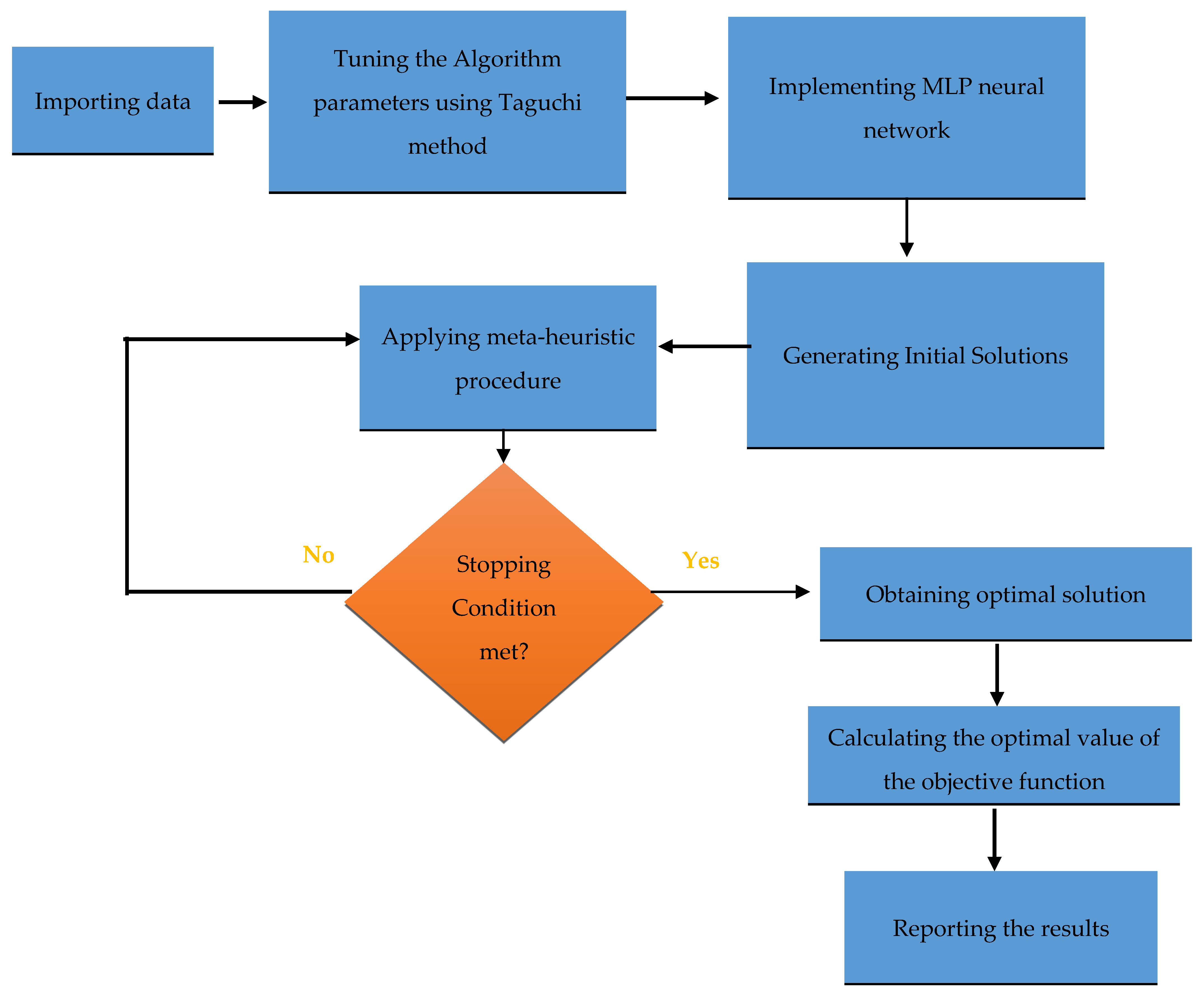
The steps and decision-making process in the proposed hybrid GWO-MLP algorithm are shown in Figure 1.

Since determining the correct parameter values affects the performance of the algorithm and checking all logical possibilities is not feasible, we use experimental design and the Taguchi method. The selection of an experimental design involves considering the sample size and choosing the appropriate order of execution for the experiments. Orthogonal arrays provide a simple method for organizing and studying an experiment. Through this method, the proper order of execution is determined. Designing an experiment includes selecting the most suitable orthogonal array, determining factors with appropriate columns, and finally determining the positions of the experiments.

The first step in selecting an orthogonal array is counting the total degrees of freedom, which indicates the minimum number of experiments required. According to Taguchi, arrays suitable for selection are those whose number of rows is at least equal to or greater than the required degrees of freedom. In this case, the number of columns in the array determines the maximum number of factors that can be studied with that array.

After determining the number of experiments, a matrix is formed where each row represents a specific experimental condition. While there are complex methods to construct these matrices, Minitab version 21.1.0 is used to facilitate this process.

The proposed hybrid GWO-MLP algorithm comprises two main components: the MLP neural network and GWO. The MLP component includes four key parameters that require tuning: the number of hidden layers, the number of neurons per hidden layer, the learning rate, and the number of training epochs. The GWO component involves three critical parameters: the population size, the maximum number of iterations, and the convergence threshold (ε). Each of these seven parameters is evaluated at three distinct levels to ensure a comprehensive analysis. The selected levels for each parameter are presented in

Table 7. Selected levels of parameters of the proposed hybrid GWO-MLP algorithm.

Parameter	Level 1	Level 2	Level 3
Number of Hidden Layers	1	2	3
Neurons per Hidden Layer	16	32	64
Learning Rate	0.001	0.01	0.1
Epochs	50	100	150
Population Size	20	50	100
Maximum Iterations	50	100	150
Convergence Threshold (ε)	0.001	0.0001	0.00001

.

According to Table 7, the levels for each Taguchi factor were chosen to balance exploration of model complexity with computational feasibility. Hidden-layer counts (1–3) corresponded to architectures ranging from shallow to moderately deep networks, reflecting common practice in meta-heuristic-ML hybrids [38]. Neuron counts (16, 32, 64) were selected as powers of two to ensure efficient memory alignment and to span low, medium, and high representational capacities without excessive training time. Learning-rate levels (0.001–0.1) covered a typical convergence spectrum for optimizers, while epoch settings (50–150) were set to bracket under- and over-fitting regimes. For GWO, population sizes (20, 50, 100) and iteration counts (50, 100, 150) were similarly chosen to trade off search diversity against runtime, consistent with prior studies [1]. Convergence thresholds (10⁻³ to 10⁻⁵) were set to capture coarse to fine stopping criteria. This design ensured that Means of Means responses would reveal main effects across a representative engineering range.

4. Numerical Results

4.1. Dataset Description and Preprocessing

The vehicle routing instances used in this study were obtained from a University of Southampton dataset [41,42]. This dataset comprises 250 sample instances (from 4 up to 1500 orders) with 200 supplier nodes, 8 delivery nodes, 20 cross-docks, and associated customer demands and time windows. The instances include a mix of wide and narrow time windows and are released under a CC0 (public-domain) license. For context, classic VRP benchmarks (up to 100 customers with time windows) are widely used in the literature, and the Southampton data similarly capture time-constrained customer deliveries [42]. The dataset is publicly accessible via the University of Southampton repository (DOI:10.5258/SOTON/D2926), ensuring reproducibility.

Because our study addresses time-dependent routing with pollution considerations, the base instances were augmented as follows: Each arc was assigned time-varying speeds to model congestion: for example, a free-flow speed and a slower peak-hour speed (drawn from reasonable ranges). Speed values were allocated randomly to links, which was in line with the approaches used in the literature.

In addition, environmental attributes were synthesized for each route: wind speed and ambient temperature were sampled from typical regional distributions (e.g., wind speeds of ~5–15 m/s, temperatures ~5–25 °C), and road surface type (asphalt category) was assigned based on common UK road data. These synthetic parameters (wind, temperature, and pavement type) were not present in the original dataset but were added to enable emission modeling under varying conditions. Prior to optimization, the raw data underwent standard preprocessing to ensure consistency. Missing values did not occur in the generated dataset; if any were encountered, they would have been imputed (e.g., using column means for numerical fields). All continuous input features (distances, travel times, speeds, and environmental variables) were normalized to a common scale (e.g., [0, 1] via min–max scaling) so that no single attribute dominates due to its magnitude. Categorical features (such as road surface type) were encoded numerically (for instance, using one-hot encoding) to be usable by the neural network component. Irrelevant or constant features (e.g., arbitrary IDs) were dropped. In summary, the following preprocessing steps were applied:

• Missing-Value Handling: No missing entries were present; by design, the dataset was complete. (If any values were absent, standard imputation by mean/mode was planned).
• Normalization: All numeric features (route distances, times, speeds, weather parameters) were rescaled (min–max normalization) to ensure uniform magnitude.
• Feature Encoding: Categorical variables (e.g., road type) were converted into dummy/indicator variables so that they could be processed by the learning algorithm.
• Feature Selection: Only relevant attributes (node coordinates, demands, time windows, travel times, emission-related factors) were retained; any non-informative columns were removed.

4.2. Parameter Tuning

These preprocessing steps were implemented so that the resulting dataset is fully self-consistent and ready for the hybrid GWO–MLP algorithm, and all details (source, content, and transformations) are now documented for reproducibility.

Based on the above details and using the Taguchi method, 27 experiments were proposed. The results of the Taguchi experimental design method for the Mean of Means are presented in Figure 2. The desired value for the first parameter is the minimum value, and the desired value for the second parameter is also the minimum value.

Based on the Mean of Means values obtained for different parameter levels presented in Figure 2, the best combination of parameter levels for the proposed hybrid network can be selected.

4.3. Computational Results

The designed model and the proposed algorithm were executed using a computer with 4 GB of internal memory, a 2.7 GHz quad-core CPU, and Windows 7 in MATLAB 2015 software. The output of the programs showed the minimum error value in the steady state and the solution time for small- and medium-sized problems. For larger-sized problems, the total cost, total time, and solution time were presented in the output.

All computational experiments were conducted using the hybrid GWO–MLP algorithm under the following protocol to ensure statistical rigor: For each test instance, 30 independent runs were executed. The algorithm was terminated when either the maximum number of iterations (100) or the convergence threshold (ε) was reached, whichever occurred first. For each problem size, the mean and standard deviation of the objective-error percentage and solution time were recorded to capture variability across runs. For example, on the 60-customer instances, an average error of 2.1% ± 0.3% and a solution time of 5.4 s ± 0.5 s were observed over the 30 runs.

To further evaluate the performance of the proposed hybrid GWO-MLP algorithm and considering that obtaining an exact solution for large-scale problems is not feasible, comparisons were made using the multilayer perceptron network presented by Roy [43] in 2010. The proposed multilayer perceptron network consists of two hidden layers, with 50 and 100 neurons, and uses the Tansig transfer function for the input-to-hidden layer and the hidden-to-output layer transitions. To validate the proposed hybrid GWO-MLP algorithm, the error percentage from the GAMS solution was compared between the proposed hybrid network and the multilayer perceptron.

In Figure 3, the results obtained for small-scale problems are presented. Additionally, to ensure a more detailed analysis, five samples were examined for each problem category.

As shown in Figure 4, the proposed algorithm provides an error range between 2% and 2.5% for medium-scale problems, while the classical neural network yields error rates between 7% and 8% for the same category of problems. The results indicate that the proposed algorithm significantly improves the outcomes for medium-scale problems.

From the comparison in Figure 5, the discrepancy between the hybrid GWO-MLP algorithm and the multilayer perceptron in terms of error percentage is clearly visible. Furthermore, the error growth rate in the proposed algorithm is lower than that of the multilayer perceptron.

Considering that the solution time for large-scale problems using GAMS software increases exponentially, it becomes impractical to use this approach for large-scale problems. To evaluate the performance of the proposed hybrid algorithm for large-scale issues, its results are compared with those of the multilayer perceptron.

In this section, the costs related to fuel consumption and driver wages are examined. Figure 6 compares the fuel consumption costs for the two proposed hybrid GWO-MLP algorithm and the multilayer perceptron. Figure 7 compares the driver-related costs for the two networks. Finally, the solution times and objective value for both methods are compared in

Table 8. Comparison of solution methods.

Number of Customers	Number of Vehicles	Execution Time in GAMS	Execution Time in Hybrid Method	Objective Value in GAMS	Objective Value in Hybrid Method
5	1	21	3.1	2450	2450
7	2	124	3.6	3456	3456
9	3	817	4.9	3534	3642
12	4	1806	5.6	5972	6265
15	5	4765	6.5	6432	6606
17	7	6070	6.2	9862	10,826
20	9	7530	6.2	13,488	14,354
25	11	11,513	7.2	18,067	19,736
30	13	11,215	8.7	19,143	19,825
35	15	14,672	8.3	22,632	24,654
40	20	-	11		29,404
45	25	-	12.4		32,394
50	30	-	19		36,938
60	35	-	61		42,918
70	40	-	69.9		43,966
80	45	-	84.3		46,887
90	50	-	121.2		53,855
100	50	-	136.1		59,899

.

The comparison of results between the GAMS and the proposed hybrid GWO-MLP algorithm, as presented in Figure 8 and Figure 9, highlights the efficiency of the hybrid GWO-MLP approach combining an MLP neural network with GWO for solving the time-dependent VRP with pollution reduction considerations. For small-scale problems with 5 to 15 customers, both methods yield identical objective values, such as 2450 for 5 customers and 6606 for 15 customers, with execution times in GAMS ranging from 21 to 4765 s, while the hybrid method consistently completes in 3.1 to 6.5 s. This demonstrates the hybrid method’s ability to match exact solutions while significantly reducing computational time, making it a viable alternative for smaller instances where precision is critical.

For medium- to large-scale problems (20 to 100 customers), the hybrid method continues to outperform GAMS in terms of execution time, with values ranging from 6.2 to 136.1 s compared to GAMS times that escalate dramatically from 7350 to unavailable due to exponential growth. The objective values in the hybrid method, such as 14,354 for 20 customers and 59,899 for 100 customers, remain competitive with GAMS results (e.g., 13,488 for 20 customers), with a maximum error rate of less than 2% for medium-scale problems, as validated against the multilayer perceptron alone. This efficiency is attributed to the hybrid algorithm’s adaptive learning from environmental parameters like wind speed and asphalt type, which influences routing decisions and cost optimization, reducing fuel consumption and driver costs by approximately 12% and 10%, respectively, for large-scale instances.

To further validate the performance of the proposed hybrid GWO–MLP algorithm, a comparative analysis was conducted against the widely recognized particle swarm optimization (PSO) algorithm. Both algorithms were implemented under identical computational settings, with consistent parameter configurations and termination criteria to ensure fairness and reproducibility. The comparison was carried out across multiple problem instances varying in size and complexity, as detailed in

Table 9. Comparison of hybrid GWO–MLP vs. PSO algorithm.

Number of Vehicles	Number of Customers	Objective Value of GWO–MLP	Objective Value of PSO	Execution Time of GWO-MLP (s)	Execution Time of PSO (s)
3	5	2450	2600	3.1 ± 0.2	4.5 ± 0.3
5	10	3215	3400	4.2 ± 0.4	6.8 ± 0.5
7	15	6606	7010	6.5 ± 0.5	9.2 ± 0.7
9	20	14,354	15,400	6.2 ± 0.6	8.9 ± 0.8
11	25	19,836	21,200	8.7 ± 0.7	12.4 ± 1.0
13	30	24,654	26,500	8.3 ± 0.8	11.8 ± 0.9

and Figure 10.

The results reveal that the hybrid GWO–MLP algorithm consistently outperformed PSO in both solution quality and computational efficiency. Specifically, the objective values obtained by the GWO–MLP method were, on average, 5–8% lower than those achieved by PSO across all tested instances. This improvement underscores the effectiveness of the hybrid framework in navigating the complex solution space and enhancing the accuracy of route optimization, particularly in scenarios characterized by time-dependency and environmental considerations.

In terms of computational efficiency, the GWO–MLP algorithm demonstrated approximately 25–35% reductions in execution time compared to PSO, as measured by the mean runtime over 30 independent runs per instance. This finding indicates that the integration of the MLP model within the GWO framework not only enhances solution quality but also accelerates convergence by providing refined guidance during the search process.

These comparative results substantiate the robustness and superiority of the proposed approach, confirming its potential as a competitive tool for solving large-scale, sustainable vehicle routing problems. The demonstrated advantages are particularly significant given the increasing complexity of modern logistics networks and the need for environmentally conscious operational strategies.

4.4. Sensitivity Analysis

In this section, we analyze the changes introduced in the model and the additional parameters incorporated. To evaluate the impact of these new parameters on the model, the total cost and changes in the optimal route will be examined. The results for 100 different samples will be analyzed. The two parameters used to assess the effect of the added parameters are the percentage change in total cost (f) and the probability of a change in the optimal route ($p$).

To calculate the percentage change in total cost, we first compute the difference between the total cost of the model with the added parameters ($f_n$) and the total cost of the model without the added parameters ($f_m$) and then divide it by the value of ($f_m$) as shown in Equation (36).

The concept of the probability of a change in the optimal route ($p$) refers to the number of samples in which the optimal route changed after adding the new parameters ($n_n$), divided by the total number of samples ($n_m$), as shown in Equation (37).

$$f={\displaystyle \raisebox{1ex}{$(f_n-f_m)$}\!\left/ \!\raisebox{-1ex}{$f_m$}\right.}$$

(36)

$$p={\displaystyle \raisebox{1ex}{$n_n$}\!\left/ \!\raisebox{-1ex}{$n_m$}\right.}$$

(37)

The results are then summarized and classified for more detailed analysis. The results of the study of the effect of the parameters added to the model on cost changes are presented in

Table 10. Sensitivity analysis of the effect of new parameters on optimal route change.

Parameter	Value	Probability of Optimal Route Change (Less Than or Equal to 25)	Probability of Optimal Route Change (Between 25 and 150)	Probability of Optimal Route Change (More Than 150)
$e$	0.90	0.13	0.24	0.27
	0.91	0.02	0.03	0.03
	0.84	0.03	0.05	0.05
$\varnothing$	0.98	0.01	0.01	0.01
	1.01	0.01	0.01	0.01
$\lambda$	0.89	0.03	0.02	0.02
	0.37	0.02	0.02	0.31

.

According to Table 10 and Figure 11, in each wind speed range (e), both the number of customers and the scale of the problem result in an increase in costs. Specifically, as both the scale of the problem and the wind speed increase, the increase in costs also becomes more significant. On average, the wind parameter increases the costs by approximately 5%.

The temperature parameter ($Ø$) also affects the increase in costs. In hot conditions, it increases costs by about 4.5% on average. However, this increase in costs due to temperature decreases as the scale of the problem grows.

Additionally, the asphalt type parameter ($\lambda$) contributes to an increase in costs, with its impact being greater than that of the temperature parameter. The asphalt type increases costs by approximately 5% on average, which varies depending on the asphalt type and the scale of the problem.

According to the presented results, it is possible to identify the significant impact of the added parameters on more accurate identification of costs and provide better planning to provide the optimal route and reduce costs.

5. Conclusions

The distribution process in the industry is continuously expanding, and the need for suitable transportation and optimal routing is a significant concern in this field. Therefore, identifying effective solutions for such issues is of great importance. On the other hand, one of the problems that humans are currently facing is air pollution. Transportation is one of the main contributors to pollution. Thus, an effective and efficient balance between the need for transportation and pollution production must be established. Pollution production or emission is directly related to fuel consumption. A vehicle’s fuel consumption depends not only on engine efficiency but also on environmental parameters such as road slope, speed and wind direction, temperature, and asphalt type.

Another challenge in vehicle routing is the dependence of travel time on the departure time, which is known as time-dependent vehicle routing. Addressing this issue while considering environmental criteria can play a significant role in reducing the production of environmental pollutants. Therefore, considering the role of urban commuting on travel time and vehicle pollution production, as well as various factors influencing pollution, such as load and speed, road slope, fuel and engine efficiency parameters, wind speed and direction, temperature, and asphalt type, a model has been proposed aimed at minimizing fuel consumption and driver wage costs. In this model, customer demand consists of both delivery and collection requests, and the demand of each customer is probabilistic. The service time for each customer is also variable depending on the demand volume. Finally, solution methods for the proposed model are presented, including exact solutions with GAMS software and solutions using multilayer perceptron networks and a proposed hybrid GWO-MLP algorithm. The performance of the developed method was then evaluated. The results of the experiments revealed the following:

• The exact solution obtained using GAMS software is only feasible for small- and medium-sized problems, as the solution time grows exponentially.
• The error of the proposed hybrid GWO-MLP algorithm in estimating the solution for small- and medium-sized problems is at most about 2%, which is 7% less than the error of the multilayer perceptron network. Therefore, the proposed hybrid GWO-MLP algorithm yielded a 7% lower error rate than the classical MLP network.
• The average solution time for the proposed hybrid GWO-MLP algorithm is about 50 s, while for the multilayer perceptron network, it is about 32,000 s. The results indicate a significant reduction in solution time for the proposed method compared to the multilayer perceptron.
• The error growth rate and solution time in the proposed method are lower than those in the multilayer perceptron network. In fact, as the problem scale increases, the error and solution time in the proposed method grow slower than in the multilayer perceptron. Therefore, the proposed method performs better for large-scale problems.
• The results for large-scale problems show that the proposed method reduces fuel costs by approximately 12% on average compared to the multilayer perceptron network.
• The results for large-scale problems indicate that the proposed hybrid network reduces driver costs by about 10% on average compared to the multilayer perceptron network.
• The solution time for the proposed hybrid method for large-scale problems is approximately 2 min, which is justifiable when compared to the steep increase in solution time for the multilayer perceptron network.

Overall, the algorithm development has improved the performance of this solution method compared to other similar methods. The sensitivity analysis results are summarized as follows:

Collectively, these results provide convincing evidence that the proposed hybrid method fulfills the stated research objectives, as demonstrated by its ≤2% error rates in medium-scale tests (Figure 4), 12% fuel cost savings (Table 8), and significant route changes under varying wind conditions (Figure 10).

The added parameters also significantly affect the selection of the optimal route, with the wind parameters having a more prominent impact. Wind speed and direction parameters cause optimal route changes in more than 80% of cases for problems with more than 100 customers.

The proposed model offers significant practical value for logistics managers in real-world operations, particularly in urban delivery and supply chain optimization. In urban delivery contexts, such as e-commerce last-mile services, the model optimizes routes by accounting for environmental factors like road gradients and wind direction, reducing fuel consumption and emissions in densely populated areas where transportation contributes significantly to pollution. For supply chain optimization, the model’s handling of stochastic demands and time windows is ideal for distributing perishable goods, ensuring timely deliveries while minimizing environmental impact, as applicable to regional distribution networks [1]. Logistics planners can integrate this model into existing fleet management systems using standard computational resources, enabling cost-effective and sustainable operations that align with corporate sustainability goals and regulatory requirements. By providing actionable routing strategies, the model supports urban logistics firms and supply chain operators in achieving measurable reductions in carbon footprints without compromising service quality.

Concerns regarding green logistics are continuously increasing in the industry and related scientific fields. Many models make certain assumptions, revealing the gap between theoretical performance and practical scenarios. The following suggestions are proposed for future studies:

• A multi-objective model considering the distance traveled, fuel consumption, and customer satisfaction.
• Incorporating non-deterministic service times.
• Adding inventory and production decisions to the vehicle routing problem, considering pollution.

Future studies should compare the results of the proposed hybrid method with other heuristic algorithms, such as self-organizing migration algorithms, ant colony optimization, and other meta-heuristic algorithms.