Ecological Light Pollution (ELP) Scale as a Measure of Light Pollution Impact on Protected Areas: Case Study of Poland

Abstract

Light pollution is a rapidly growing environmental challenge, with the global brightness of the night sky increasing by an average of 9.6% per year. This study assessed the ecological impact of artificial light at night (ALAN) on protected areas in Poland, including all 23 national and 125 landscape parks, from 2012 to 2023. Based on VIIRS satellite radiance data and modelled sky surface brightness (Sa), we developed and applied the Ecological Light Pollution (ELP) scale, which classifies areas into four classes of ecological impact: strong (ELP-A), pronounced (ELP-B), noticeable (ELP-C), and weak or none (ELP-D). The analysis revealed that 38.5% of protected areas are affected by artificial skyglow at levels classified as ELP-B or ELP-C. Under cloudy conditions, which intensify light pollution effects, 22% of national parks and 41.8% of landscape parks fell into these classes. Notably, Wielkopolski National Park exhibited the most pronounced impact (ELP-B) even under clear skies, primarily due to its proximity to the Poznań metropolitan area. In contrast, Bieszczadzki and Białowieski National Parks recorded near-natural darkness (ELP-D). These light pollution effects can disrupt nocturnal species’ behaviour, reduce biodiversity, and degrade opportunities for dark-sky tourism. The findings emphasise the need for targeted mitigation, including stricter outdoor lighting regulations, formal dark-sky protection zones, and public education to preserve protected areas’ ecological integrity and tourism potential.

1. Introduction

Light pollution (LP) is one of the fastest-growing environmental problems. According to estimates, the brightness of the night sky background increased globally by an average of 9.6% per year from 2011 to 2022 [1]. Until recently, it was believed that this increase was several times smaller and did not exceed 3% per year for the entire globe [2]. Such significant changes are mainly caused by excessive or improper use of artificial lighting at night (ALAN), which is emphasised by one of the definitions, which describes light pollution as “human-made alteration of outdoor light levels from those occurring naturally” [3]. Other definitions most often refer to the impact of ALAN on the external environment. However, it should be noticed that there is also “indoor light pollution”, which can be emitted, for example, from TV screens, computers and other devices that are standard equipment in homes [4,5].

Light pollution includes several key forms that differ in their source and nature of impact. Artificial skyglow, resulting from the scattering of light in the atmosphere, particularly affects urban areas and their immediate surroundings [2,6], i.a. by reducing the visibility of stars, disorienting numerous species of organisms and causing a decrease in landscape and astrotourism values [7]. The brightness of artificial skyglow depends on various factors, such as cloud cover, concentration of different types of aerosols and ground albedo [8,9]. It is a growing threat to wildlife worldwide [10]. Over the past few years, artificial skyglow has caused a doubling of ground illumination intensity during the new moon, which is extremely important for the proper course of biological processes. This effect occurs in 77.1% of the world’s protected areas and about 20% of regions with high biodiversity for mammals, birds and amphibians [11]. Moreover, fewer than 20% of the world’s Key Biodiversity Areas (KBAS) have night skies that remain entirely unaffected by artificial light; around two-thirds are fully exposed to artificially brightened skies, and only about one-third remain altogether free from skyglow reaching the zenith [12]. It shows that light pollution can severely affect wildlife even in the most critical areas for biodiversity, mainly due to skyglow. Artificial skyglow, visible from several kilometres away, significantly affects wildlife, particularly crepuscular and nocturnal species by altering patterns of organismal activity and disrupting natural daily, lunar, and seasonal rhythms [10]. For example, nightjars (Caprimulgus europaeus) show increased nocturnal flight activity under artificially brightened skies compared to natural ones [13]. Prey detection is improved under these conditions. However, these birds prefer natural moonlight to artificial skyglow [14]. Artificial skyglow affects not only terrestrial animals. Experimental studies have shown that even freshwater fish, such as European perch (Perca fluviatilis), experience reduced melatonin concentrations when exposed to low-intensity artificial light [15]. Recent studies have identified at least 136 animal species negatively affected by light pollution. This demonstrates that such a form of anthropogenic disturbance impacts individual organisms and propagates across multiple levels of ecological organisation, ultimately threatening the integrity of entire ecosystems [11,16]. This highlights the particular vulnerability of protected areas to light pollution.

In addition to skyglow, other forms of light pollution may also occur in protected areas, such as light trespass, which occurs when artificial light reaches places where it is not desired, e.g., interiors of apartments or areas of high natural value [17], or glare, which may impede visual perception, posing a threat to both people, e.g., in road traffic, and migrating animals [18]. Over-illumination should also be mentioned, which means using too intense lighting, often without practical justification [19].

The impact of light pollution is multidimensional and can cause negative consequences for both ecosystems and human health [20]. In humans, exposure to artificial light at night is associated with sleep disorders, reduced melatonin synthesis and an increased risk of lifestyle diseases such as obesity, diabetes, depression or cancer [21,22]. In LP ecosystems, it disrupts the circadian cycles of animals, disrupting migration, reproduction or feeding [23,24]. Examples include nocturnal insects, attracted by artificial light sources, which leads to their disorientation, energy depletion and, consequently, a reduction in the population of many species [25]. Animal behavioural disorders are also observed among many species of birds [26], bats [27] and sea turtles [28]. Plants exposed to long-term and intense ALAN also exhibit developmental abnormalities [29]. It should be added that the biodiversity of ecosystems is influenced not only by direct lighting from lighting infrastructure but also by urban light haze, which can reach many kilometres beyond the administrative boundaries of cities [16]. It also hinders the development of astrotourism, especially one of its branches called dark-sky tourism, because it degrades the quality of the night sky and makes it difficult to conduct practical astronomical observations.

The impact of artificial sky glow, including sky glow, on protected areas worldwide has been studied for over two decades. The results of studies using satellite tools [2,6] were particularly helpful in the initial diagnosis of the impact of artificial sky glow on national parks and other areas. They showed that a large part of protected areas, especially in developed countries (Europe, Turkey, the Caribbean, South and East Asia, the eastern part of the United States), may be affected by the consequences of LP generated from neighbouring areas. To calculate the percentage of threatened areas, the Protected Areas Light Pollution Indicator (PALI) and the Protected Areas Human Influence Indicator (PAHI) were developed and applied to protected areas around the world [30]. Analyses of LP changes in 1992–2010 were also performed on over 170 thousand protected areas on all continents [31]. A study was also prepared, including data for skyglow illuminance, taking into account the World Database on Key Biodiversity Areas, to assess the extent of skyglow illuminance in marine and terrestrial areas important for biodiversity conservation [11]. In addition to the “global” analyses performed for protected areas around the world, in recent years, similar, detailed studies have also been carried out in individual countries, e.g., in Korea [32], China [33], or Balkans [34].

In Poland, the problem of light pollution is becoming increasingly visible due to the development of lighting infrastructure, including replacing traditional light sources with LEDs. The first comprehensive study of this phenomenon, included in the publication “Light Pollution in Poland—Report 2023” [35], shows that the total level of radiance in 2022 was 6% higher than for 2012–2021. However, this increase was much more significant for some communes and amounted to over 50%. Consequently, many rural areas, which until recently had a relatively low level of LP, experienced an expansion of this phenomenon during the decade under study, mainly due to the impact of urban light halos. The analysis also showed that the problem of the effects of urban halos may also affect naturally valuable areas, including national and landscape parks (NP and LP, respectively), which may reduce their biodiversity and, as a result, their natural and tourist values. At the same time, social awareness and legal regulations in this area remain insufficient, highlighting the need for urgent educational and legislative actions and precise monitoring of the impact of light pollution on naturally valuable regions.

This study aims to propose a scale, referred to in the further part of the publication as Ecological Light Pollution (ELP), which allows us to determine the impact of light pollution, understood here as artificial skyglow, on local ecosystems. This impact, potentially reducing biodiversity and night landscape values, degrades the tourist potential of protected areas. Our classification differs from most previous classifications of light pollution levels, which are based on the ratio to the naturally dark sky level or threshold values for the visibility of astronomical objects (e.g., the visibility of the Milky Way) [2,6], in that it includes thresholds based on the activity of selected animal groups while also taking into account the influence of cloud cover on the change in the impact of urban glow (see Section 2.2.1). The detailed objectives of the work are to: (a) indicate national and landscape parks particularly exposed to the impact of light pollution in the form of light glow from nearby cities; (b) create a ranking of national and landscape parks in terms of the adopted classification of the ELP scale; (c) indicate recommendations for protected areas, aimed at minimising the impact of LP on nocturnal ecosystems.

The ELP scale has significant potential as a tool supporting the development of public policies and planning the functioning of protected areas. Its use allows for monitoring long-term trends in light pollution and identifying areas with the highest priority for protection from artificial light. It can be the basis for formulating nature conservation policy objectives at local and regional levels—e.g., by defining high-risk zones for fauna biodiversity, including nocturnal fauna, or designating areas requiring modification of lighting systems.

In planning practice, the ELP can support decision-making processes in local spatial development plans, studies of conditions and directions of municipal development and assessments of the impact of investments on the environment, considering the impact of artificial light on ecosystems. It can also be used to justify the introduction of dark sky protection zones or special lighting regimes in the surroundings of national and landscape parks. This approach, based on the scientifically justified classification of the ecological impact of ALAN, is already used in international initiatives to protect the night landscape, including in biosphere reserves and certified dark sky parks.

The study covers all national parks (23 in number) and landscape parks (125 in number) established in Poland by the date of publication of the work, within their official external borders, without the buffer zone. Information on the intensity of light pollution was obtained from processing satellite data from the Visible Infrared Imaging Radiometer Suite (VIIRS) instrument mounted on board the American meteorological satellite Suomi National Polar-orbiting Partnership (SNPP) and the sky brightness model. The time frame of the analysis covers the years 2012–2023.

2. Materials and Methods of Research

2.1. Protected Areas in Poland

The nature protection system in Poland is regulated by the Act of 16 April 2004 on nature protection [36], which defines a hierarchical model of protection and distinguishes its three types: forms of area protection, forms of object protection and species protection of plants, animals and fungi. The strictest forms of area protection are national parks (23 in Poland) and nature reserves (1441), while landscape parks (125), protected landscape areas (389) and Natura 2000 areas (over a thousand) are characterised by more flexible regulations. Area forms of protection are supplemented by object protection forms, among which are natural monuments (over 30 thousand), ecological sites (over 7 thousand), and nature and landscape complexes and documentation sites (several hundred) [37]. Such a protection system is intended to protect natural, landscape and cultural values against degradation, while at the same time enabling sustainable development and use of natural resources, i.a. for tourism purposes. The latter are mainly developed in national parks (over 14 million visitors in 2019 [38]) and landscape parks, due to their large area (less than 9.5% of the country’s area) and unique ecological and landscape values as well as spatial accessibility [39,40].

In Poland, by the time of publication of this paper, 23 national parks had been established with a total area of approximately 336 thousand ha, constituting 1.1% of the country’s area (Figure 1). They were created in regions distinguished by exceptional landscapes and natural values, including valuable ecosystems or endemic species of plants and animals. National parks (NP) include mountain ecosystems (e.g., Tatrzański NP), forest ecosystems (e.g., Białowieski NP), wetland ecosystems (e.g., Biebrzański NP), as well as ecosystems of dune communities (e.g., Słowiński NP). They are managed by the principle of strict, active, and landscape protection, which allows for preserving their original character while ensuring tourist access, with traffic strictly controlled and limited to trails or paths designated for this purpose.

Strict protection covers about 25% of the total area of all national parks. They are mainly forest areas (about 60%), waters cover about 10%, and the remaining area includes agricultural land and other forms of land. Each park must have a buffer zone, an area designated to protect against external threats resulting from human activity [41]. The total area of buffer zones of Polish national parks is larger than the parks themselves and amounts to over 430 thousand ha, which is 1.4% of the country’s area. Selected information about each park can be found in Appendix A (

Table A1. National parks in Poland.

No.	Name of National Park (NP)	Abbr.	Area	LT	LA	Sac	Sao
I	Babiogórski NP	BabPN	3394	592	0.174	21.2	20.5
II	Białowieski NP	BiaPN	10,529	352	0.033	21.8	21.8
III	Biebrzański NP	BiePN	59,736	2066	0.035	21.7	21.7
IV	Bieszczadzki NP	BPN	29,208	994	0.034	21.9	22.0
V	Drawieński NP	DPN	11,251	470	0.042	21.7	21.5
VI	Gorczański NP	GPN	7023	257	0.037	21.2	20.4
VII	Kampinoski NP	KamPN	38,533	3232	0.084	20.4	18.9
VIII	Karkonoski NP	KrkPN	5954	340	0.057	20.9	19.9
IX	Magurski NP	MPN	18,626	652	0.035	21.7	21.5
X	Narwiański NP	NPN	6807	437	0.064	21.1	20.2
XI	Ojcowski NP	OPN	2156	176	0.082	20.3	18.7
XII	NP “Bory Tucholskie”	PNBT	4598	183	0.077	21.0	20.1
XIII	NP Gór Stołowych	PNGS	6334	218	0.047	21.5	21.1
XIX	NP Ujście Warty	PNUW	8078	243	0.038	21.1	20.3
XV	Pieniński NP	PiePN	2371	444	0.055	21.1	20.3
XVI	Poleski NP	PolPN	9770	354	0.036	21.7	21.5
XVII	Roztoczański NP	RPN	8476	294	0.035	21.7	21.5
XVIII	Słowiński NP	SPN	32,317	1118	0.035	21.7	21.5
XIX	Świętokrzyski NP	SwPN	7687	365	0.048	21.0	20.0
XX	Tatrzański NP	TPN	21,153	1331	0.063	21.1	20.3
XXI	Wielkopolski NP	WPN	7594	1063	0.140	19.9	18.1
XXII	Wigierski NP	WigPN	15,098	725	0.048	21.5	21.1
XXIII	Woliński NP	WolPN	10,908	671	0.062	21.2	20.5

Abbr.—short name of the park; Area—total area of park [ha]; L_T—median of total radiance from the area of park in 2013–2023 [10⁻⁹ W/cm²·sr]; L_A—median of the radiance per unit of park area in 2013–2023 [10⁻⁹ W/cm²·sr/km²]; S_ac—median of the S_a value in park for cloudless sky in 2013–2023 [mag/arcsec²]; S_ao—median of the S_a value in park for overcast sky in 2013–2023 [mag/arcsec²].

).

Landscape parks are a more flexible and less rigorous legal form of nature protection than national parks. There are 125 of them in Poland (Figure 1), and their total area exceeds 2.6 million ha, 8.4% of the country’s area. Landscape parks protect areas of high landscape and natural and cultural value while enabling economic activity that aligns with the principles of sustainable development. They also protect ecosystems associated mainly with forest and agricultural areas, including river valleys and mountain areas. Some landscape parks act as buffer zones for national parks, creating a buffer between areas requiring strict protection and areas transformed by human activity.

An example is Zaborski Landscape Park, the buffer zone for the “Bory Tucholskie” National Park. Buffer zones are essential for the nature protection system because they limit the impact of external factors related to urbanised areas, including various types of environmental pollution, on the core areas of national parks. Detailed data on each Polish landscape park can be found in Appendix A (

Table A2. Landscape parks in Poland.

No.	Name of Landscape Park (LP)	Abbr.	Area	LT	LA	Sac	Sao
1	Barlinecki LP	BarPK	11,694	686	0.059	21.3	20.6
2	Barlinecko-Gorzowski LP	BGPK	12,263	513	0.042	21.4	20.8
3	Bielańsko-Tyniecki LP	BTPK	6359	1311	0.206	20.8	19.6
4	Bolimowski LP	BolPK	23,567	772	0.033	21.4	20.9
5	Brodnicki LP	BPK	16,936	193	0.011	20.7	19.6
6	Brudzeński LP	BruPK	3127	3304	1.057	19.3	17.4
7	Cedyński LP	CedPK	29,434	1356	0.046	21.4	20.9
8	Chełmiński LP	ChelmPK	21,242	2350	0.111	20.8	19.7
9	Chełmski LP	ChelPK	16,205	608	0.038	21.4	21.0
10	Chęcińsko-Kielecki LP	CKPK	19,789	1277	0.065	19.7	17.8
11	Chojnowski LP	ChojPK	6870	2919	0.425	20.4	19.0
12	Ciężkowicko-Rożnowski LP	CRPK	18,247	1072	0.059	21.0	20.2
13	Cisowsko-Orłowiński LP	COPK	20,687	1461	0.071	21.0	20.0
14	Ciśniańsko-Wetliński LP	CWPK	51,461	1072	0.021	21.3	20.7
15	Czarnorzecko-Strzyżowski LP	CSPK	25,654	1687	0.066	21.9	21.9
16	Dłubniański LP	DPK	11,158	880	0.079	20.5	19.2
17	Drawski LP	DraPK	42,292	2176	0.051	21.6	21.2
18	Gostynińsko-Włocławski LP	GWPK	37,078	1194	0.032	21.5	21.1
19	Górznieńsko-Lidzbarski LP	GLPK	27,531	114	0.004	21.4	20.9
20	Gorzowski LP	GPK	3075	1804	0.587	21.1	20.2
21	Iński LP	IPK	17,575	757	0.043	21.5	21.2
22	Jaśliski LP	JPK	25,878	157	0.006	21.2	20.5
23	Jeleniowski LP	JelPK	4218	945	0.224	21.8	21.7
24	Kaszubski LP	KaszPK	33,201	3029	0.091	21.0	20.1
25	Kazimierski LP	KazPK	14,974	1053	0.070	21.0	20.1
26	Kozienicki LP	KozPK	25,921	292	0.011	20.8	19.6
27	Kozłowiecki LP	KozłPK	5934	1264	0.213	20.8	19.8
28	Kozubowski LP	KozubPK	6170	225	0.036	21.4	20.9
29	Krajeński LP	KrajPK	74,983	3850	0.051	21.3	20.7
30	Krasnobrodzki LP	KrasPK	9457	335	0.035	21.7	21.5
31	Krzczonowski LP	KrzczPK	12,427	445	0.036	21.4	20.8
32	Krzesiński LP	KrzePK	8579	413	0.048	21.3	20.7
33	Książański LP	KsPK	3072	373	0.121	20.3	18.8
34	Lednicki LP	LPK	7618	561	0.074	20.8	19.7
35	Łagowsko-Sulęciński LP	LSPK	5439	682	0.125	21.0	20.0
36	Łomżyński LP Doliny Narwi	LPKDN	7394	341	0.046	21.3	20.7
37	Mazowiecki LP im. Czesława Łaszka	MPKCL	15,755	2596	0.165	21.6	21.3
38	Mazowiecki LP	MazPK	56,258	57	0.001	21.4	20.8
39	Miedzichowski LP	MiedzPK	1437	2502	1.741	20.0	18.4
40	Nadbużański LP	NadPK	73,645	1835	0.025	20.9	19.8
41	Nadmorski LP	NadmPK	17,828	1641	0.092	21.2	20.4
42	Nadnidziański LP	NadnPK	22,889	3301	0.144	21.4	21.0
43	Nadwarciański LP	NadwarPK	13,649	687	0.050	21.1	20.2
44	Nadwieprzański LP	NadwiepPK	6231	569	0.091	20.8	19.7
45	Nadwiślański LP	NadwisPK	42,121	5222	0.124	20.6	19.4
46	LP Cysterskich Kompozycji Krajobrazowych Rud Wielkich	PKCKKRW	49,582	6338	0.128	20.4	19.0
47	LP Dolinki Krakowskie	PKDK	20,466	3091	0.151	20.6	19.3
48	LP Ujście Warty	PKUW	19,592	582	0.030	21.1	20.2
49	LP Beskidu Małego	PKBM	47,152	7960	0.169	20.1	18.4
50	LP Beskidu Śląskiego	PKBS	38,276	642	0.017	21.0	20.0
51	LP Chełmy	PKCh	15,752	5928	0.376	21.0	20.0
52	LP Dolina Baryczy	PKDBar	85,722	997	0.012	20.2	18.7
53	LP Dolina Bystrzycy	PKDBys	8585	376	0.044	20.6	19.3
54	LP Dolina Dolnej Odry	PKDDO	6079	350	0.058	21.0	20.0
55	LP Dolina Jezierzycy	PKDJ	8066	3932	0.487	20.6	19.4
56	LP Dolina Kamionki	PKDKam	2053	871	0.424	21.9	22.0
57	LP Dolina Słupi	PKDSlup	37,514	1730	0.046	21.5	21.1
58	LP Doliny Bobru	PKDB	10,599	1096	0.103	20.8	19.6
59	LP Doliny Sanu	PKDSan	27,728	293	0.011	21.0	20.1
60	LP Góry Opawskie	PKGO	9587	767	0.080	20.9	19.9
61	LP Gór Słonnych	PKGSlon	56,188	695	0.012	20.4	18.9
62	LP Gór Sowich	PKGSow	8158	2311	0.283	21.7	21.5
63	LP Góra Św. Anny	PKGSA	5617	430	0.077	20.8	19.7
64	LP Góry Łosiowe	PKGŁ	4874	1461	0.300	21.5	21.1
65	LP im. gen. Dezyderego Chłapowskiego	PKGDCh	17,325	961	0.055	21.3	20.8
66	LP Lasy Janowskie	PKLJ	40,122	4568	0.114	20.7	19.6
67	LP Lasy nad Górną Liswartą	PKLnGL	51,113	521	0.010	21.4	20.8
68	LP Łuk Mużakowa	PKLM	18,716	1113	0.059	21.2	20.6
69	LP Mierzeja Wiślana	PKMW	4118	963	0.234	21.1	20.2
70	LP Międzyrzecza Warty i Widawki	PKMWiW	25,368	5196	0.205	20.6	19.3
71	LP Nadgoplański Park Tysiąclecia	PKNPT	12,814	250	0.020	20.5	19.1
72	LP Orlich Gniazd	PKOG	61,069	1022	0.017	21.1	20.2
73	LP Pasma Brzanki	PKPB	15,428	1182	0.077	21.5	21.1
74	LP Podlaski Przełom Bugu	PKPPB	30,691	3295	0.107	21.4	20.9
75	LP Pogórza Przemyskiego	PKPP	60,562	528	0.009	21.4	21.0
76	LP Pojezierza Iławskiego	PKPI	25,589	2255	0.088	21.6	21.4
77	LP Pojezierze Łęczyńskie	PKPL	12,025	1330	0.111	21.5	21.1
78	LP Promno	PKP	3374	620	0.184	21.7	21.6
79	LP Puszcza Zielonka	PKPZ	12,224	1013	0.083	21.8	21.7
80	LP Puszczy Knyszyńskiej im. prof. Witolda Sławińskiego	PKPKWS	73,190	755	0.010	20.4	19.0
81	LP Puszczy Rominckiej	PKPR	14,865	69	0.005	21.0	20.0
82	LP Puszczy Solskiej	PKPS	29,411	373	0.013	20.7	19.5
83	LP Stawki	PKS	1727	1567	0.907	21.2	20.4
84	LP Sudetów Wałbrzyskich	PKSW	6195	389	0.063	21.4	20.8
85	LP Wysoczyzny Elbląskiej	PKWE	13,417	1212	0.090	21.1	20.2
86	LP Wzgórz Dylewskich	PKWD	7170	2671	0.373	19.9	18.1
87	LP Wzniesień Łódzkich	PKWL	14,552	197	0.014	21.7	21.5
88	Poleski LP	PolPK	5320	5376	1.011	21.1	20.2
89	Południoworoztoczański LP	PRPK	20,250	1609	0.079	21.0	20.1
90	Popradzki LP	PopPK	53,419	820	0.015	21.7	21.6
91	Powidzki LP	PowPK	24,887	618	0.025	21.4	20.8
92	Przedborski LP	PrzedPK	16,432	1048	0.064	21.2	20.5
93	Przemęcki LP	PrzemPK	21,201	1610	0.076	21.0	20.1
94	Przemkowski LP	PrzemkPK	22,901	432	0.019	21.3	20.7
95	Pszczewski LP	PszczPK	9724	1214	0.125	20.3	18.8
96	Rogaliński LP	RogPK	12,723	798	0.063	20.2	18.7
97	Rudawski LP	RudPK	15,708	1021	0.065	20.9	19.8
98	Rudniański LP	RudnPK	5910	615	0.104	20.9	19.8
99	Sieradowicki LP	SieradPK	12,252	1954	0.159	21.2	20.5
100	Sierakowski LP	SierakPK	30,918	1216	0.039	21.6	21.4
101	Skierbieszowski LP	SkierbPK	35,394	584	0.016	20.7	19.5
102	Sobiborski LP	SobPK	11,160	1158	0.104	21.3	20.7
103	Spalski LP	SpalPK	13,013	426	0.033	21.8	21.7
104	Stobrawski LP	StobPK	60,486	1014	0.017	20.8	19.7
105	Strzelecki LP	StrzelPK	12,681	592	0.047	21.1	20.3
106	Suchedniowsko-Oblęgorski LP	SOPK	19,895	888	0.045	20.3	18.9
107	Sulejowski LP	SulPK	17,026	2648	0.156	21.1	20.3
108	Suwalski LP	SuwPK	6338	383	0.060	21.8	21.9
109	Szczeciński LP	SzczPK	11,290	880	0.078	20.9	19.9
110	Szczebrzeszyński LP	SzczebPK	19,379	269	0.014	21.7	21.6
111	Szczeciński LP “Puszcza Bukowa”	SPKPB	9118	676	0.074	21.7	21.5
112	Ślężański LP	SlęzPK	7678	759	0.099	21.1	20.2
113	Śnieżnicki LP	SniepPK	27,618	5124	0.186	19.8	18.0
114	Tenczyński LP	TenPK	15,154	1768	0.117	21.4	20.8
115	Trójmiejski LP	TrojPK	20,247	6012	0.297	19.7	17.9
116	Tucholski LP	TPK	36,572	983	0.027	21.4	20.8
117	Wdecki LP	WdDP	20,411	967	0.047	21.4	20.9
118	Wdzydzki LP	WdzPK	18,046	1449	0.080	21.4	21.0
119	Welski LP	WelPK	20,074	1019	0.051	20.8	19.7
120	Wiśnicko-Lipnicki LP	WLPK	14,231	205	0.014	21.4	21.0
121	Wrzelowiecki LP	WrzePK	5006	647	0.129	21.2	20.5
122	Zaborski LP	ZPK	34,981	1216	0.035	20.9	19.8
123	Załęczański LP	ZałPK	14,497	1867	0.129	21.5	21.1
124	Żerkowsko-Czeszewski LP	ZCPK	15,839	1918	0.121	21.1	20.3
125	Żywiecki LP	ZywPK	35,853	686	0.019	21.3	20.6

Abbr.—short name of the park; Area—total area of park [ha]; L_T—median of total radiance from the area of park in 2013–2023 [10⁻⁹ W/cm²·sr]; L_A—median of the radiance per unit of park area in 2013–2023 [10⁻⁹ W/cm²·sr/km²]; S_ac—median of the S_a value in park for cloudless sky in 2013–2023 [mag/arcsec²]; S_ao—median of the S_a value in park for overcast sky in 2013–2023 [mag/arcsec²].

).

Another protected area category is the world biosphere reserves established under the UNESCO-MAB (Man and Biosphere) programme, of which over 750 have been established in 136 countries. There are 11 such facilities in Poland, but they have not yet received formal legal protection, so they still operate in a discretionary formula [37]. Biosphere reserves aim to promote and achieve a lasting balance between the natural environment and the development of human resources and cultural values. For this reason, they have enormous potential, especially for areas located in buffer and transit zones of biosphere reserves to protect and display the values of the unpolluted night sky and night landscape. To understand the size and scale of the light pollution phenomenon, it is necessary to study its changes in the last decade and propose methods for determining the degree of light pollution in areas where astrotourism activities are carried out. A publication introducing the Tourist Light Pollution scale (TLP) is being prepared. Such a scale will allow for the creation of a classification of protected areas, particularly biosphere reserves, from the astrotourism perspective, and above all, the development of recommendations for the optimal planning and effective development of dark sky tourism products in these areas. There are already a few dark sky parks and reserves operating in the world within biosphere reserves, and their goal is to develop sustainable astrotourism, educational activities on the adverse effects of ALAN and protection of ecosystems from the impact of light pollution. The proposed activities will promote the values of the night and build solid foundations for the durability and functioning of the biosphere based on natural environmental resources, with active human participation.

Polish national and landscape parks have already been the research subject regarding light pollution measurements. However, most often, measurements were limited to a single protected area, e.g., Tatrzański National Park [42]. For this purpose, ground measurement methods were often used, including Sky Quality Meters (SQM), and in some cases, thematic atlases or GIS simulations.

Analyses were also carried out based on satellite data. The initial diagnosis of the degree of artificial light pollution in all Polish national parks was made in 2015 [43] based on data presented in The First World Atlas of the artificial night sky brightness [6]. However, the most comprehensive attempt to capture the ecological impact of light pollution on the areas of national parks was presented in the previously mentioned study, Light Pollution in Poland—Report 2023 [35]. It offered a preliminary concept of ELP based on data from 2012 to 2022. As a result, three parks were indicated where the impact of light pollution may have noticeable consequences for the local ecosystems. The results of our study are an extension of this concept, both theoretically and spatially, because, in addition to national parks, they also cover the areas of landscape parks.

2.2. Ecological Light Pollution (ELP) Scale

2.2.1. Determining the Brightness of the Night Sky’s Glow

The first mass assessments of the night sky brightness were made in the 1990s at the International Dark-Sky Association (IDA) initiative and, of course, concerned cloudless skies. These assessments were made using simple visual methods, consisting of observing astronomical objects against the background of the night sky and estimating their brightness based on them, which is why they are often called astronomical methods. The simplest observational method, commonly used in creating night sky brightness maps, is determining the number of visible stars in a precisely defined sky area (counting stars, CS) [44]. Another simple, frequently used method of determining the brightness of the night, cloudless sky is determining the so-called limiting magnitude (NELM) of observed stars. It consists of searching for the faintest star visible in a given sky area using the averted vision method [45].

The first scale, allowing for the assessment of the brightness of the night, cloudless sky, was developed in 1976 by Berry [46]. This scale is based on simple sky observations and requires no significant observational experience. It is a six-point scale: point 1 means the sky is densely strewn with stars up to the horizon, with the Milky Way visible on clear nights also up to the horizon, point 6 implies the visibility of only a few hundred faintly visible stars, the sky is bright and faded over the entire surface. This scale is developed by the nine-point Bortle scale [47], which is most commonly used today; the subsequent points are based on the visibility of various astronomical objects.

All of the scales listed above were created for the needs of astronomy enthusiasts. Defining a specific Berry or Bortle scale class allows us to determine the potential possibility of observing a given class of astronomical objects in a particular location. Moreover, these scales apply only to cloudless skies. However, classifying a given area according to these scales does not allow us to determine how the glow in a given location may affect local ecosystems. The ELP scale and its classes that we propose approach the problem from the point of view of ecology, not astronomy.

2.2.2. Activity of Selected Groups of Organisms

Most artificial light pollution classification is based on the visibility of various celestial objects. This study proposes a novel framework to evaluate the potential thresholds at which artificial light at night negatively affects multiple wild animal species, selected as model organisms due to their well-documented responses to this environmental stressor.

For various living organisms, the beginning of the day is associated with the phenomenon of dawn, i.e., the natural brightening of the night sky associated with the approaching sunrise. Often, from the point of view of an organism located at ground level, only the zenith area is visible from the entire sky. Therefore, it is believed that the increase in brightness of this part of the sky is treated as the end of the night period and the beginning of daytime activity [48].

However, the moment at which the sky reaches a certain (“night-ending”) brightness can be significantly altered by artificial light. Experiencing light pollution can cause a sky to appear as bright as it would at dawn many hours earlier in the natural environment, or to be permanently brighter than at twilight. Therefore, we decided to use the relationship between animal activity and night sky brightness as the basis for a new, ecologically oriented scale for determining the impact of light pollution on the environment: the Ecological Light Pollution Scale (ELP). This scale takes into account light pollution intensity classes. They were proposed based on the behaviour of the following groups of organisms:

• Birds. Many bird species begin their dawn chorus before sunrise. Ambient light, temperature, weather conditions, and seasonality influence morning singing behaviour. However, changes in light intensity between day and night remain among the most significant factors triggering birds to sing [49]. In Europe, some of the earliest species to begin singing include the blackbird (Turdus merula), the song thrush (Turdus philomelos), and the European robin (Erithacus rubecula), which typically start their vocalisations more than an hour before sunrise [50]. However, birds sing significantly earlier in light-polluted areas, sometimes even several hours before sunrise [50,51].
• Bats. European bats are predominantly nocturnal, beginning their activity around sunset and returning to their roosts shortly before sunrise [52]. Due to their nocturnal behaviour, bats are highly affected by light pollution, but their responses vary depending on foraging behaviour and habitat context. In some cases, bats that forage on insects attracted to streetlights may benefit from artificial light at night (ALAN). However, most European species respond negatively to ALAN, particularly near roosts and drinking sites. Additionally, narrow-space foraging species tend to avoid artificially lit areas while foraging [53].
• Insects. Many invertebrate species are nocturnal. For example, within the order Lepidoptera, which includes butterflies and moths, approximately 75% to 85% of species are nocturnal [54]. Furthermore, studies on insect community diel patterns have revealed that, on average, insect activity is 31.4% higher at night than during the day [55]. Research on moths has shown that most species reach peak activity shortly after sunset, with some exhibiting an additional peak just before sunrise. However, most of their activity occurs earlier at night, indicating a gradual decline in activity in the hours leading up to dawn [56,57].

Another natural factor that determines the behaviour of various organisms at night is the full moon’s light, or rather its absence near the new moon. Dark, moonless nights are conducive to the reproduction of several species of mammals (e.g., badgers) [58] or amphibians (e.g., salamanders or frogs) [59]. The full moon’s light also disturbs the balance of the hunter-prey system, which is particularly visible in eutrophic water bodies [60]. The above examples allow us to establish the limiting brightness of the artificial skyglow, which becomes at least as necessary (if not more critical) than natural factors that brighten the sky, such as dawn or the full moon.

2.2.3. Determination of ELP Classes

To specify the sky brightness at the times of day when specific animal species become active or fall asleep, data from an area practically free from light pollution, such as the Gorczański National Park, on the Suhora peak (1000 m) were used. Inside the park, there is the Astronomical Observatory of the University of the Commission of National Education (UKEN) in Kraków, where a measuring station (referred to as SUH) of the Light Pollution Monitoring Laboratory (LPML) of the Kraków University of Technology has been operating since the beginning of 2015. The SQM-LE meter installed at this station performs continuous measurements of the sky surface brightness at the zenith (hereinafter referred to as S_a). Simultaneously, photos of the sky taken by an all-sky camera allow for determining, among other things, the degree of cloudiness during the measurement of the S_a at any time in the past, starting from the beginning of the station’s operation.

To determine the value of S_a at the moment when birds start singing, bats or nocturnal insects stop their activity, marked as S_ad, moonless and completely cloudless nights in May 2022 and 2023 were used. Of these, nights were selected in which the S_a value was equal to 21.8 mag/arcsec² near local midnight. This is the maximum S_a value at the SUH measuring station in May, determined based on an analysis of many years of measurements, guaranteeing the absence of any other factors influencing the sky brightness, apart from the twilight effect.

When these conditions are met, the following values are obtained:

• S_ad = 20.6 mag/arcsec², corresponds to the “awakening” of the song thrush and robin, about 90 min before sunrise [48,61];
• S_ad = 19.0 mag/arcsec², corresponds to the “awakening” of the blackbird, 75 min before sunrise [62];
• S_ad = 21.5÷17.9 mag/arcsec², hiding of nocturnal insects, 60–120 min before sunrise [57].

In the case when the only light source in the sky is the moon, previously conducted field measurements have shown that the ground illuminance of the brightened sky reaches a value equal to the ground illuminance of the full moon at a S_a value of 17.3 mag/arcsec² (hereinafter referred to as S_am) [63].

Considering the given S_ad and S_am values, a method for determining the potential ecological impact of light pollution in the form of artificial skyglow can be proposed. As a result, a four-level ecological light pollution scale (ELP) was defined, which is related to the brightness of the night skyglow (this scale does not consider the direct impact of local lighting). The given thresholds for individual classes were established based on the S_ad values for the above-mentioned groups of organisms:

• >20 mag/arcsec²: very weak or no ecological impact (ELP-D).
• 19–20 mag/arcsec²: noticeable ecological impact (ELP-C).
• 17–19 mag/arcsec²: pronounced ecological impact (ELP-B).
• <17 mag/arcsec²: strong ecological impact (ELP-A).

The above analysis shows that to determine the ecological impact of the night skyglow in a given area, it is sufficient to measure the zenith value S_a with the estimated percentage of cloud cover at the zenith. To avoid the error related to the uncertainty of this estimation, it is best to perform two measurements: a cloudless sky and an overcast one. The section determined this way allows for the most reliable classification of the studied area into one of the defined ELP classes (from ELP-A to ELP-D). More reliable conclusions are obtained after plotting the full dependence of S_a on the percentage of cloud cover in the sky.

When analysing a specific case, it is essential to know whether it is in the ecological light pollution zone (ELP-A, ELP-B, or ELP-C) only in the case of an overcast sky or partial cloud cover. When the examined area “falls” into the ELP-A or ELP-B zone, even for a cloudless sky, it should be considered heavily contaminated with ecological light pollution.

2.2.4. Impact of Cloud Cover on the Allocation to the Specific ELP Class

The presented values of S_a thresholds refer to the cloudless sky. However, a much more significant impact on ecosystems is the light reflected from clouds, which amplifies light pollution [64,65]. In particular, it has been shown that cloud cover increases the luminance of the night urban sky tenfold, while in rural surroundings it increases it threefold. It has also been found that cloudy nights are four times brighter in the city than cloudless, rural nights brightened by moonlight.

The sky may be frequently partially covered with clouds or overcast. For instance, in Poland, the number of cloudy days in a year (i.e., days with average cloudiness exceeding 80%) varies typically between 140 and 180, depending on location [66]. Since clouds change the value of S_a [64], their presence can also cause a change in ELP class assignment.

Based on measurements of S_a at the zenith, its value was found to change linearly with the increase in low cloud cover, expressed as a percentage of the covered sky in the meter’s field of view. It was also found that the directional coefficient of this relationship changes depending on the amount of ALAN in the environment (Figure 2) [9,67].

2.2.5. Spatial Data, Radiance and Night Light Intensity Data

The source of the night skyglow is ground-based light sources, such as urban areas, large greenhouses, industrial areas, logistics centres or national road intersections, etc. As established earlier [67], the range of ground illumination by the artificial night skyglow is greater than the size of these ground-based light sources. It depends on the value of the light-polluted sky surface brightness, the height of the cloud base and the degree of air pollution with particulate matter. Based on the above analyses, an empirical relationship was established between the size of the surface covered by the artificial skyglow and its brightness. Additionally, considering the maximum range, occurring when the sky is overcast with high clouds, a three-kilometre buffer of its impact on the surroundings was established for each ground-based light source [9]. All national parks (Appendix A, Table A1) and landscape parks in Poland (Appendix A, Table A2) were analysed, considering their location in the direct range of the artificial skyglow and the buffer described above.

The external boundaries of national and landscape parks were obtained in vector form from the central access point to spatial data and services in Poland (geoportal.gov.pl). Data processing using ArcGIS ver. 10.4 (Esri) software consisted of aggregating separate data within each protected area, removing the buffer zone, except when it was a landscape park, and standardising names. All analyses were performed within the external boundaries of large-scale protected areas, and the occupation area given in Appendix A, Table A1 and Table A2, results from our data processing. Selected data on land cover were obtained based on the Corine Land Cover data.

ELP categories are essentially thresholds applied to the values of night sky surface brightness (S_a) at the zenith. Therefore, the latter parameter is the only one required for assigning a location to a specific ELP class. Information on S_a may be acquired using a ground-based photometer (SQM). However, it will be limited only to point locations (as in Section 3.2). Alternatively, S_a can be estimated over large areas using radiative transfer models. The most commonly used one was introduced by Garstang [68] and significantly improved by Cinzano et al. [45]. The model was successfully applied by Falchi et al. [2] for calculating worldwide maps of artificial night sky brightness in the astronomical Johnson-Cousin V-band, and assuming a standard clear US62 atmosphere [69] (see [45] for details on the model setup). The dataset was later occasionally updated annually by David Lorenz of the University of Wisconsin-Madison. In this study we used a 2023 update of [2] night brightness map, kindly made available by D. Lorenz.

An essential step in producing the S_a map with the model is to indicate the location and intensity of ground light sources. Falchi et al. [2] achieved this using radiance maps based on the Visible Infrared Imaging Radiometer Suite (VIIRS) observations. VIIRS is a radiometer installed on board the Suomi-NPP polar-orbiting satellite with equatorial crossing times at 01:25 CET (night) and 13:25 CET (day). A special feature of VIIRS is sensitivity to low-level radiation in a wide spectral range between 0.5 and 0.9 µm, so-called “day-night-band”, DNB.

Depending on the application, this characteristic also imposes certain limitations. First, VIIRS provides observations only at a single moment in the night, meaning that all derived products (ELP, night sky brightness) are only relevant for that specific time. The most critical limitation is spectral sensitivity: VIIRS is not sensitive to the blue component of light; instead, it records the infrared component of radiation. This does not align with the sensitivity of the human eye (to visible light) or the receptors of various living organisms. Therefore, it should be assumed that VIIRS only provides an approximation; despite this, it is widely used due to the lack of alternatives.

Besides being essential for night sky brightness modelling, VIIRS radiances are not necessary for ELP classification. Nevertheless, we also included the raw radiance information of VIIRS to better characterise light emissions from within national and landscape parks in Poland. The analysis (Section 3.1) used a NASA operational VNP46A1 product: daily at-sensor radiances at the top of the atmosphere. The product is served at a spatial resolution of 15 s in longitude and latitude, and corrections are applied to changes in Earth surface reflectance caused by snow presence or lunar illumination [70,71]. Extensive information on cloud contamination and viewing angles is also provided.

Based on daily observations, we developed annual statistics, including the arithmetic mean of radiance (nW/cm²·sr). Final data only included cloud-free and high-quality observations, based on VNP46A1 quality assurance flags. Snow-free and snow-featuring observations at all angles were allowed. Annual composites for 2012–2023 were then used to calculate two key measures of light intensity: the sum of lights (SOL; radiance values integrated over an area) and statistical distributions of radiance values within a given area (selected percentiles of radiance).

VIIRS data were processed in Python 3 using self-developed tools. The VIIRS statistics and the night sky brightness statistics were also generated in Python, utilising its basic functionality without relying on dedicated statistical modules.

2.3. Used Units

Several units describe the phenomenon of light pollution [72]. In this paper, we use two groups of units. The first are the radiometric units. Radiometry measures optical radiation, which is electromagnetic radiation within the frequency range between 3 × 10¹¹ and 3 × 10¹⁶ Hz. The only difference between radiometry and photometry is that radiometry includes the entire optical radiation spectrum.

In contrast, photometry is limited to the visible spectrum as defined by the eye’s response. From the VIIRS/DNB data, the radiance is obtained, i.e., power per unit projected area per unit solid angle. The symbol of radiance is L, and its standard SI unit is W/m²·sr.

The second group of units are photometric units. In this paper, the surface brightness of the night sky, denoted as S_a, was measured with Unihedron SQM meters, giving the measurement results in astronomical units of magnitude per square arcsecond (mag/arcsec², mpsas). The magnitude scale is a logarithmic, relative, and inverse scale, on which an object of magnitude 0 is 100 times brighter than an object of magnitude 5. This unit determines the surface brightness of diffuse astronomical objects, such as nebulae, galaxies, comets, or just the background sky.

3. Results

As defined in Section 2.2, the Ecological Light Pollution (ELP) scale is directly related to the night sky’s brightness. The necessary measurements can be carried out at any location using a photometer or a similar device. However, such observations are limited to specific points. Modelling is required to evaluate brightness over a broader area, such as an entire country or continent. The approach used in this study [2] involves radiative transfer modelling, which simulates light propagation through the atmosphere. This method relies on VIIRS radiometry data, which provide information about the location and intensity of nighttime light sources. From this perspective, the radiance of nighttime lights is a key input for assessing night sky brightness.

Importantly, night sky brightness over a given area is not only influenced by local light sources but also by light pollution from surrounding areas. For example, a protected area may contain no internal light sources, yet still experience significant light pollution—and thus a high ELP value—due to the proximity of a nearby city. For this reason, we first report VIIRS radiance data for national parks (Section 3.1), before focusing on the primary variable of interest in this study: night sky brightness (Section 3.2).

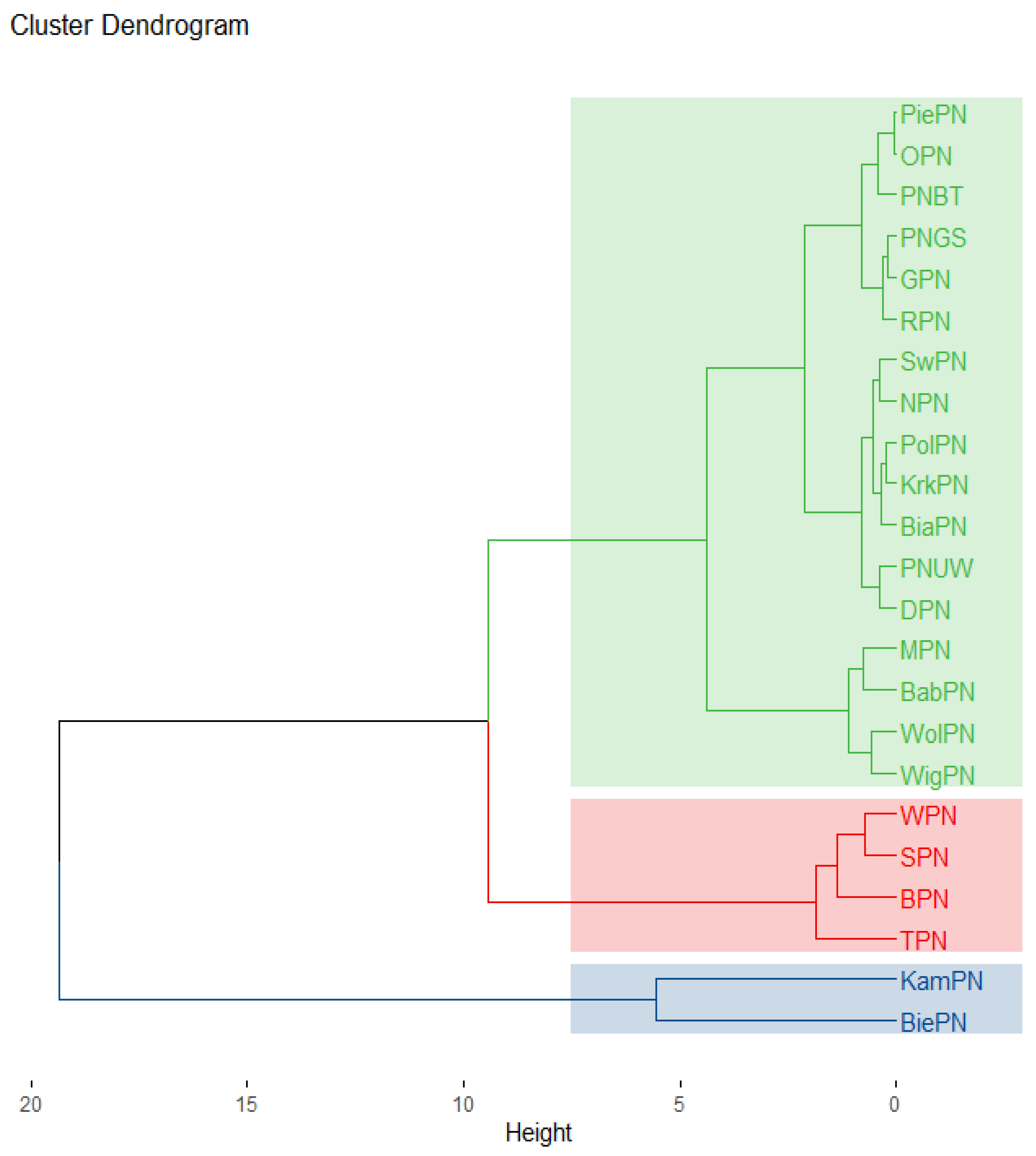
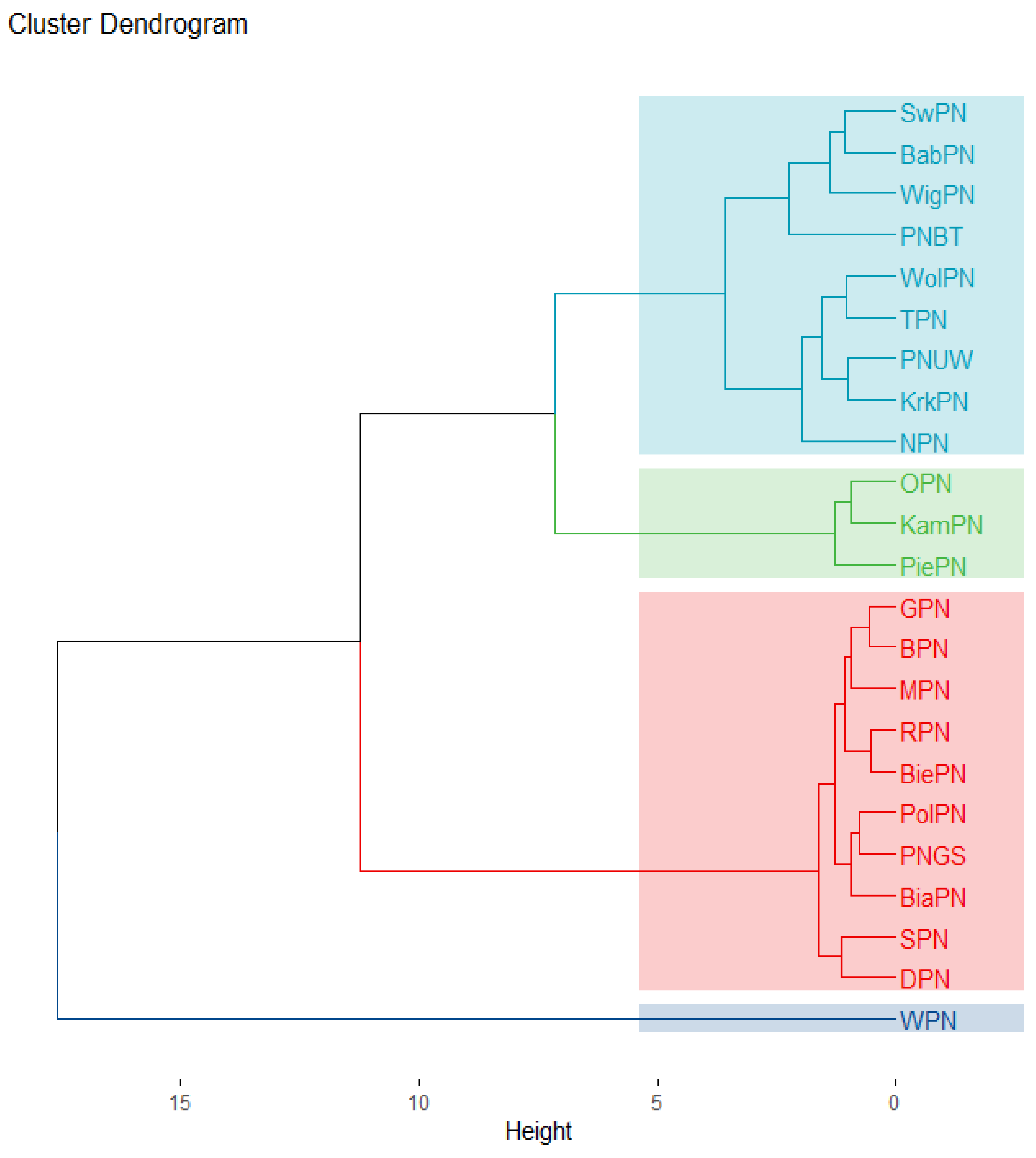
3.1. Light Emission from the Protected Areas

3.1.1. Light Emission from the Area of National Parks

The night sky’s brightness results from light emitted by artificial sources and its propagation through the atmosphere. Therefore, it is essential to characterise these emission sources first.

Their statistical analysis was done using hierarchical cluster analysis to separate groups of similar radiance values in the data sets, assuming the Euclidean metric and Ward’s minimum variance criterion (WardD2). In each case, a clear grouping of the analysed values was observed.

When the grouping parameter is the total sum of radiance from the studied area, determined from the mean annual values, three groups of national parks can be distinguished (without considering the buffer zones) (Figure A1 in Appendix B). The first group contains national parks with a high total radiance, above 2000 × 10⁻⁹ W/cm²·sr. These are Biebrzański NP (BiePN; 2090 × 10⁻⁹ W/cm²·sr) and Kampinoski NP (KamPN; 3191 × 10⁻⁹ W/cm²·sr). The second group, with radiance of about 1000, consists of Tatrzański NP (TPN; 1373 × 10⁻⁹ W/cm²·sr), Bieszczadzki NP (BPN; 1075 × 10⁻⁹ W/cm²·sr), Słowiński NP (SPN; 1126 × 10⁻⁹ W/cm²·sr) and Wielkopolski NP (WPN; 1094 × 10⁻⁹ W/cm²·sr). The remaining national parks are included in the third group, in which the radiance is less than 1000 × 10⁻⁹ W/cm²·sr.

The area of the parks can affect the obtained results, due to the potentially greater number of light sources resulting from the larger territory. Therefore, to eliminate this factor, a cluster analysis was performed on the average radiance value per unit area (Figure A2).

After considering this factor, the radiance from the area of the Wielkopolski National Park (WPN; median = 0.14 × 10⁻⁹ W/cm²·sr/km²) stands out clearly from other parks. The group containing the Pieniński NP (PiePN), Kampinoski NP (KamPN) and Ojcowski NP (OPN) is also clearly distinguished (0.08 × 10⁻⁹ W/cm²·sr/km²). It is worth noting that all of these national parks are located near large urban centres. The next group includes mainly mountain national parks, such as the Babiogórski NP (BabPN), Karkonoski NP (KrkPN), Świętokrzyski NP (SwPN) or Tatrzański NP (TPN) (0.05 ÷ 0.06 × 10⁻⁹ W/cm²·sr/km²). The lowest radiance per unit area (0.03 ÷ 0.04 × 10⁻⁹ W/cm²·sr/km²) comes from the areas of national parks such as Białowieski NP (BiaPN), Bieszczadzki NP (BPN) or Roztoczański NP (RPN). In all the studied parks, the buffer in the analysis process did not bring any significant changes.

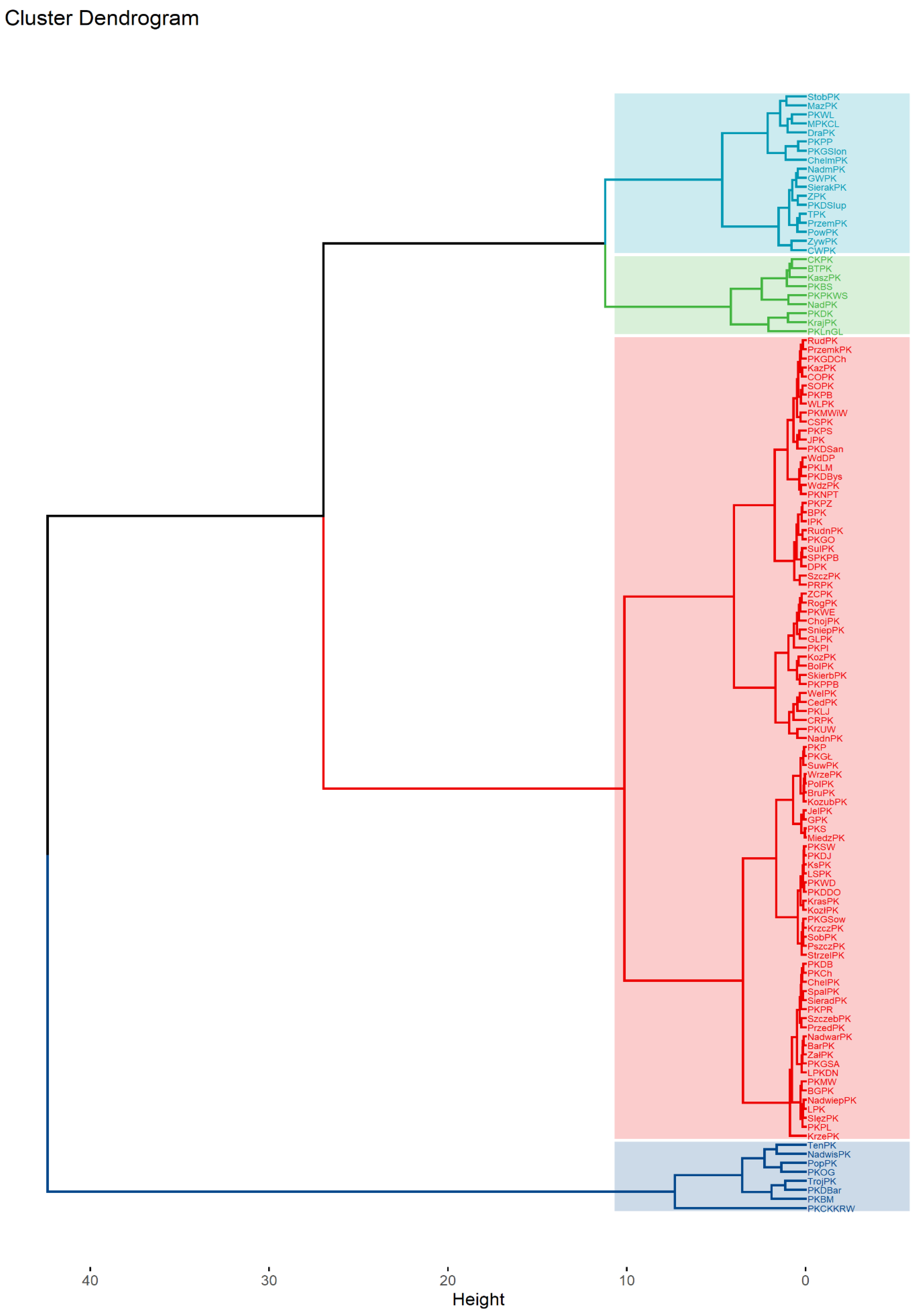
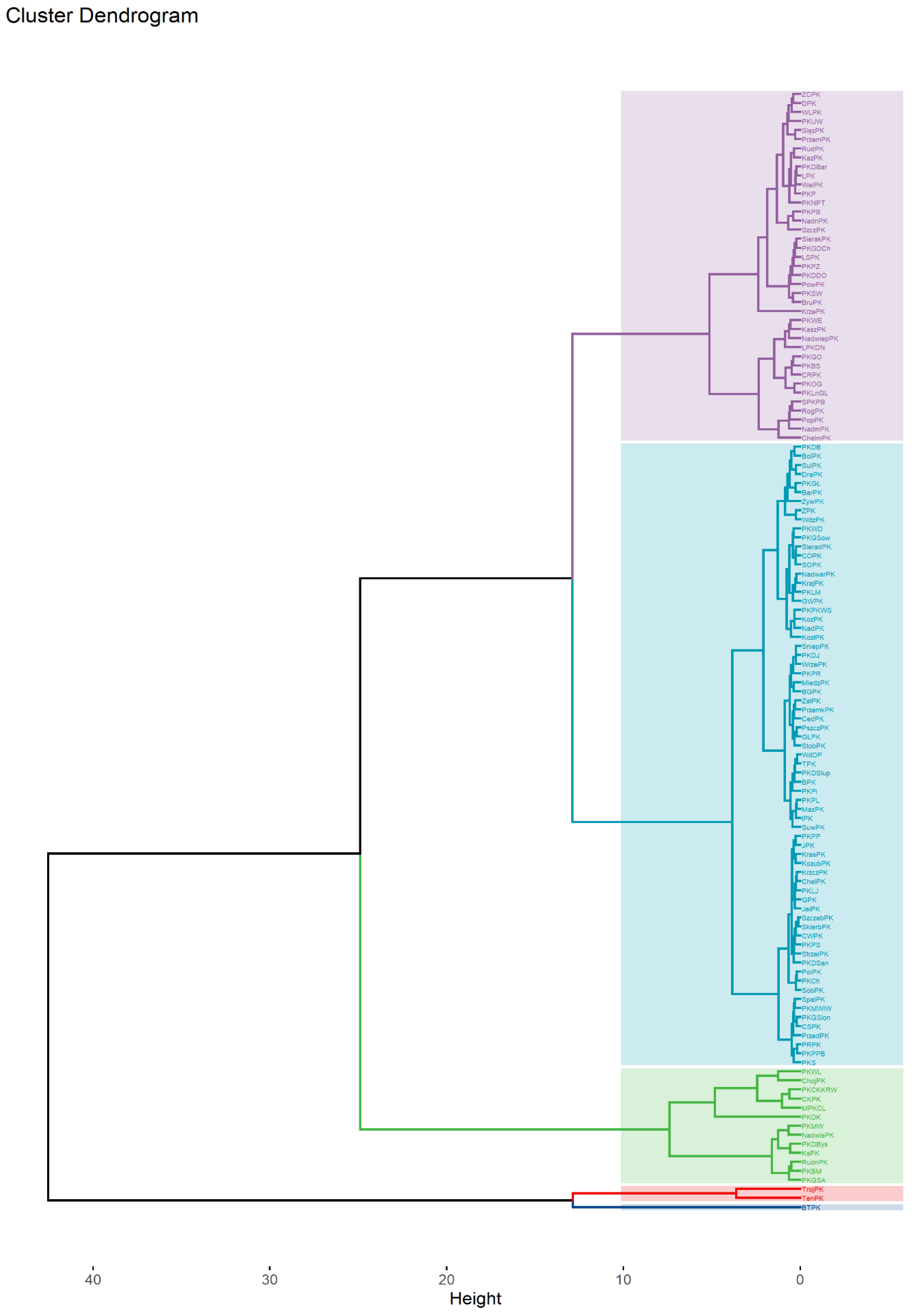
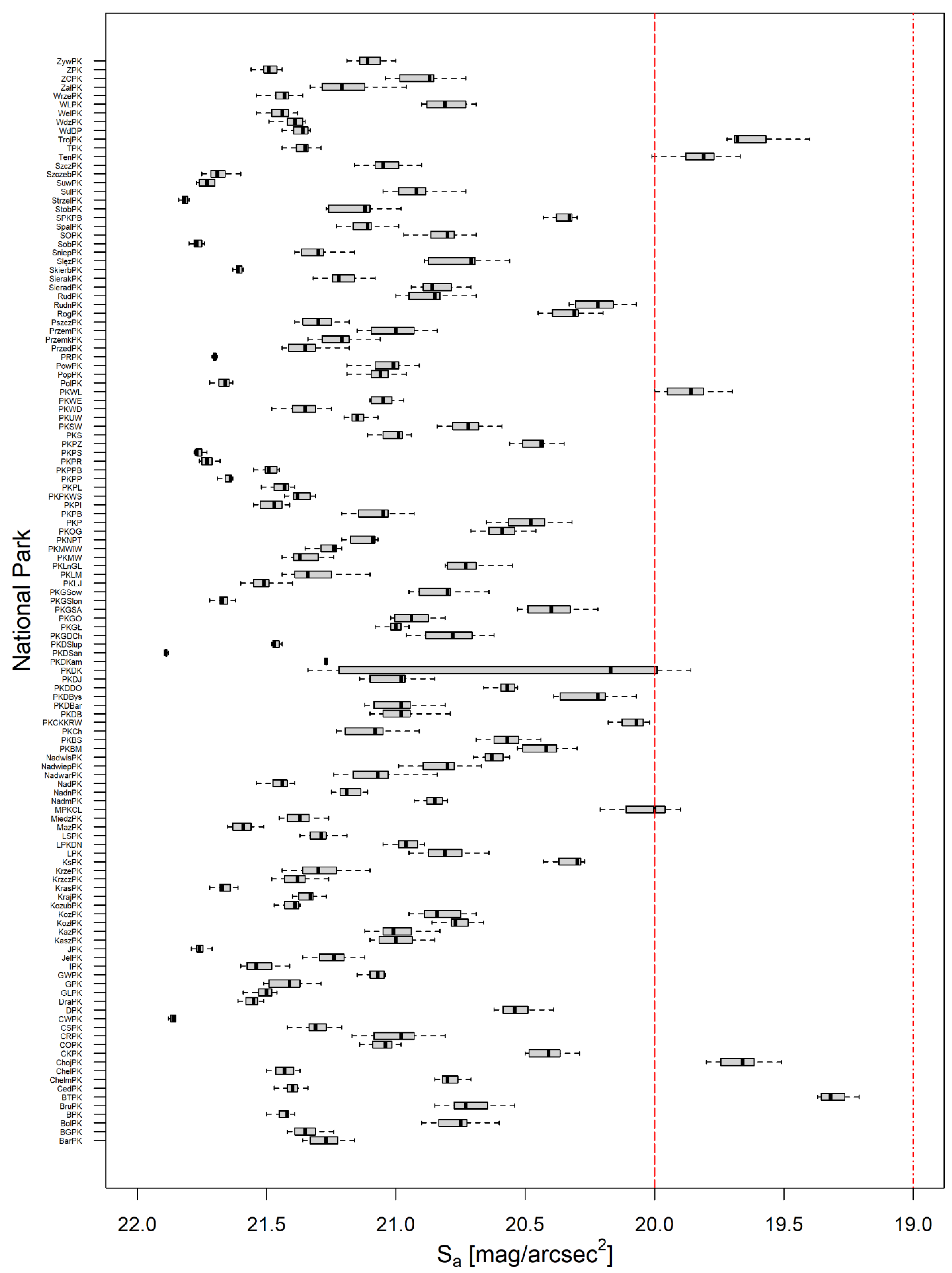
3.1.2. Radiance from Landscape Parks

Similarly to national parks, landscape parks differ in the sum of radiance. They show much greater diversity and can be divided into four groups (Figure A3). The first group (with seven members) contains landscape parks with high summed radiance, above 5000 × 10⁻⁹ W/cm²·sr. These include the Landscape Park “Cysterskie Kompozycje Krajobrazowe Rudy Wielkie” (PKCKKRW; 8000 × 10⁻⁹ W/cm²·sr), the Landscape Park Beskidu Małego (PKBM; 6338 × 10⁻⁹ W/cm²·sr) and the Trójmiejski Landscape Park (TrojPK, 6012 × 10⁻⁹ W/cm²·sr). The second group (numbering 8), with the radiance of about 10⁻⁹ W/cm²·sr, consists of, among others, Bielańsko-Tyniecki LP (BTPK; 3304 × 10⁻⁹ W/cm²·sr), Nadbużański LP (NadPK; 3301 × 10⁻⁹ W/cm²·sr), LP Puszczy Knyszyńskiej (PKPKWS; 10⁻⁹ W/cm²·sr) and Kaszubski LP (KaszPK; 3029 × 10⁻⁹ W/cm²·sr). The third group (19 in number) included landscape parks with radiance of about 2000 × 10⁻⁹ W/cm²·sr, including e.g., LP Gór Słonnych (PKGSlon; 2311 × 10⁻⁹ W/cm²·sr), Drawski Landscape Park (DraPK; 2176 × 10⁻⁹ W/cm²·sr) or Żywiecki LP (ZywPK; 1918 × 10⁻⁹ W/cm²·sr). The remaining landscape parks (90 in number) are included in the fourth group, in which the radiance is usually significantly lower than 1000 × 10⁻⁹ W/cm²·sr. While the highest sum of radiance recorded in national parks was about 1500 × 10⁻⁹ W/cm²·sr (Kampinoski NP), the “record holder” among landscape parks was the Landscape Park “Cysterskie Kompozycje Krajobrazowe Rudy Wielkie” in the Silesian Voivodeship (about 8000 × 10⁻⁹ W/cm²·sr). In total, radiance above 5000 × 10⁻⁹ W/cm²·sr was recorded in 8 landscape parks (6.5%), 44.4% of the studied areas were in the range of 1000 ÷ 5000 × 10⁻⁹ W/cm²·sr, and 49.1% of landscape parks were in the group with radiance lower than 1000·10⁻⁹ W/cm²·sr.

Based on these data, it can be assumed that more flexible operating regulations cause greater artificial light emissions from landscape parks than national parks. Similar to the case of national parks, it was necessary to determine the radiance value per unit area to confirm this initial hypothesis.

This time, five groups can be distinguished (Figure A4). The group with the highest radiance per unit area is Bielańsko-Tyniecki LP (BTPK—within the administrative borders of Kraków; 0.52 × 10⁻⁹ W/cm²·sr/km²). The second, distinguished group is Tenczyński LP (TenPK; near the administrative boundaries of Kraków; 0.34 W/cm²·sr/km² and Trójmiejski LP (TrojPK; within the administrative borders of Gdańsk; 0.30 W/cm²·sr/km². The third group includes 13 landscape parks whose radiance per unit area is within the range of 0.12 ÷ 0.20 W/cm²·sr/km², in particular Chęcińsko-Kielecki Landscape Park (CKPK; 0.15 W/cm²·sr/km²) or the LP Beskidu Małego (PKBM; 0.13 × 10⁻⁹ W/cm²·sr/km²). The fourth group (39 landscape parks) contains landscape parks whose radiance per unit area is 0.06 ÷ 0.11 W/cm²·sr/km². These include, among others, Ślężański LP (SlęzPK; 0.08 W/cm²·sr/km²) and Kazimierski LP (KazPK; 0.07 W/cm²·sr/km²). The radiance per unit area in the remaining 69 landscape parks (i.e., in as many as 55% of all landscape parks in Poland) is lower than 0.04 × 10⁻⁹ W/cm² sr/km². Considering the buffer did not significantly change the obtained data.

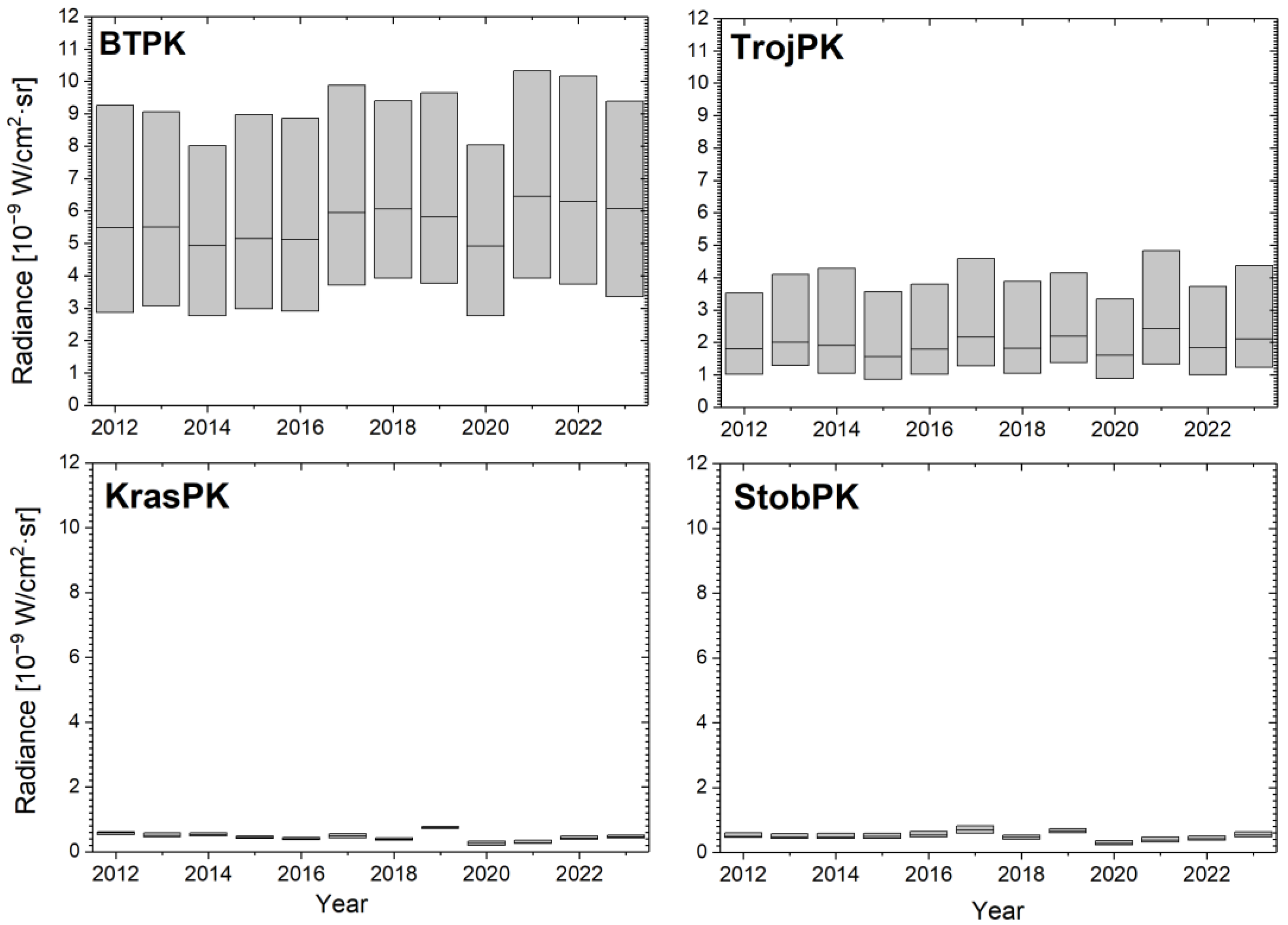
3.1.3. Radiance Changes from National and Landscape Parks in 2012–2023

Most national parks showed slight changes in radiance in the analysed period. They can be presented on the example of Kampinoski NP and Wielkopolski NP (Figure 3), which show similar periods of increase and decrease in radiance, as in most parks. Each time, 2019 was a record year, and after it, due to the COVID-19 pandemic, there was the most significant decrease in 2020. The lockdown and the extinction of some lighting installations in Poland caused this. Later years were characterised by a gradual return to the pre-pandemic situation. In some parks, the changes were analogous, but they took on relatively higher values. An example of such a park is Białowieski NP, which, like the previously mentioned ones, had a trend of increases and decreases in radiance in the same years. In this case, the difference between 2019 and 2020 was much more pronounced. In general, relative fluctuations in radiance in the analysed parks in 2012–2023 amounted to a maximum of 40–50%.

Similar changes in radiance were found for landscape parks in the period under study (Figure 4).

3.2. ELP Scale for Protected Areas

To assign individual study areas to previously defined ELP classes, box plots were created to show the distributions of S_a values in these areas.

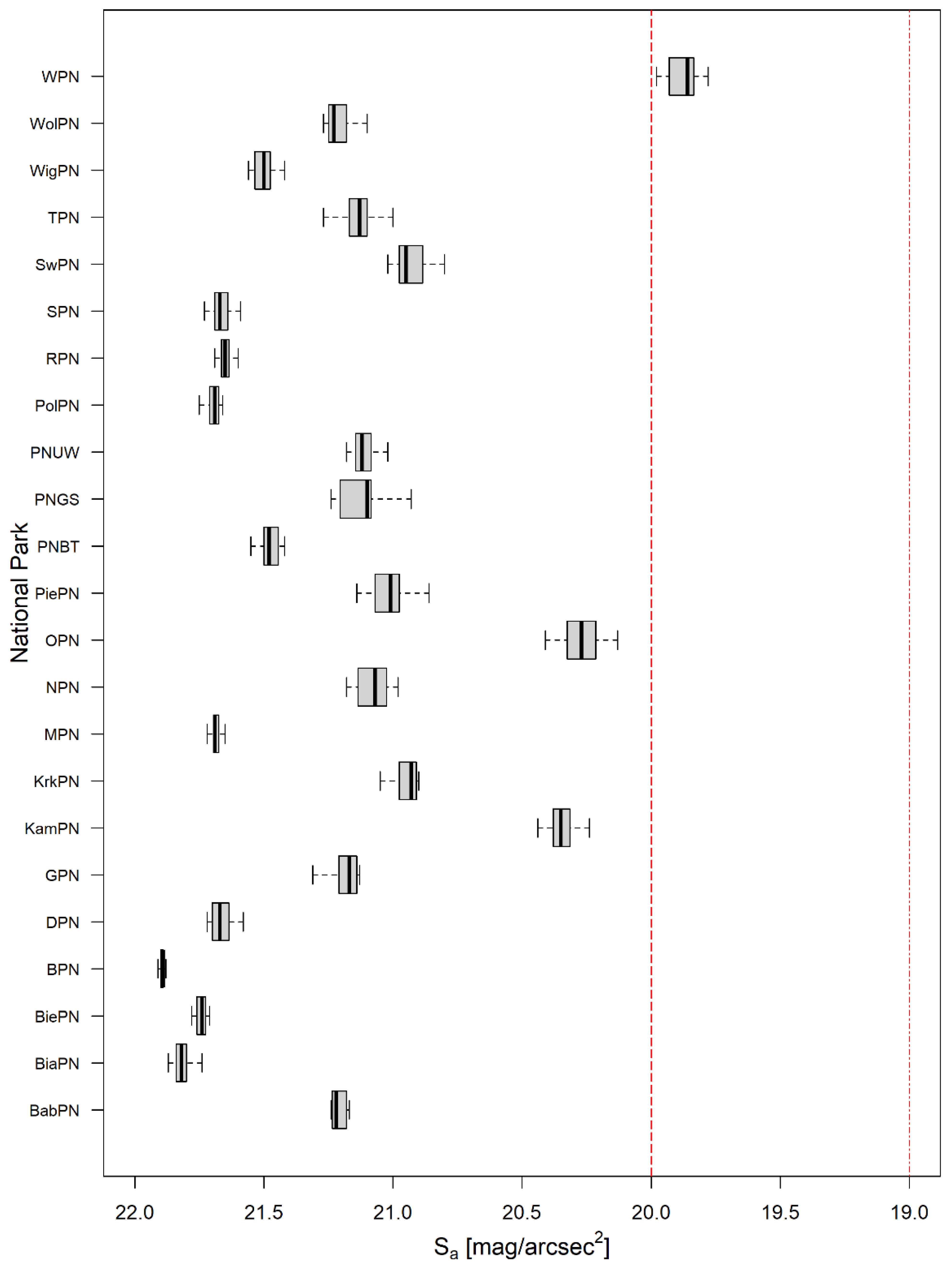
3.2.1. ELP Scale for National Parks

In the case of a cloudless sky, only the Wielkopolski National Park (WPN) was in the area of noticeable ecological impact of light pollution (a similar result was obtained when considering the buffer) (Figure A5). In two other national parks, Kampinoski NP and Ojcowski NP, the S_a value falls within the ELP-D range, but its value was close to the limit value for the ELP-C class. All three mentioned parks are located near large agglomerations, Poznań, Warszawa and Kraków, respectively. The remaining parks clearly lack LP impact on their ecosystems, but they can be divided into two groups. The first group comprises parks with a S_a value of approximately 20.9–21.3 mpsas (43.5%). The second group comprises parks with a S_a value lower than 21.5 mpsas (43.5%). The lowest S_a value, above 21.7 mpsas, was recorded in parks considered the most peripheral: Białowieski NP, Biebrzański NP and Bieszczadzki NP.

Including the cloudiness factor in the analysis increases the night sky’s brightness over the territory of almost all parks (Figure A6). As a result, the following parks are in the area of clear ecological impact of light pollution (ELP-B): Wielkopolski NP (WPN), Ojcowski NP (OPN) and Kampinoski NP (KamPN). Their example shows the dominant role of urban glow from the surrounding agglomerations. Two parks located in the mountains are in the zone of noticeable ecological impact (ELP-C): Karkonoski NP (KrkPN) and Świętokrzyski NP (SwPN). In their case, the source of the artificial skyglow is the nearby medium-sized cities, Jelenia Góra and Kielce, respectively. This result means that approximately. Notably, 22% of Polish national parks are exposed to a substantial impact of light pollution on local ecosystems.

The remaining parks are characterised by night sky brightness below the limit of noticeable impact on ecosystems. However, three distinguishable groups can be identified among them. The first are parks with S_a values of 20.0–20.5 mpsas, which cover almost 35% of all the parks studied. Some of them, especially Pieniński NP, are characterised by surface sky brightness close to the limit of noticeable impact of LP on ecosystems. The second group includes “Bory Tucholskie” NP and Wigierski NP with S_a value equal to approx. 21 mpsas (approx. 9%). The remaining group consists of parks (approx. 35%) with a S_a value higher than 21.5 mpsas. It can also be noticed that the conditions most similar to natural occur in Bieszczadzki NP (BPN) and, to a slightly lesser extent, Białowieski NP (BiaPN). Especially in the first case, adding the cloud cover factor did not increase the average sky surface brightness, but decreased it significantly. This proves that the local urban artificial sky glow has no impact on the ecosystems occurring in the Bieszczadzki National Park.

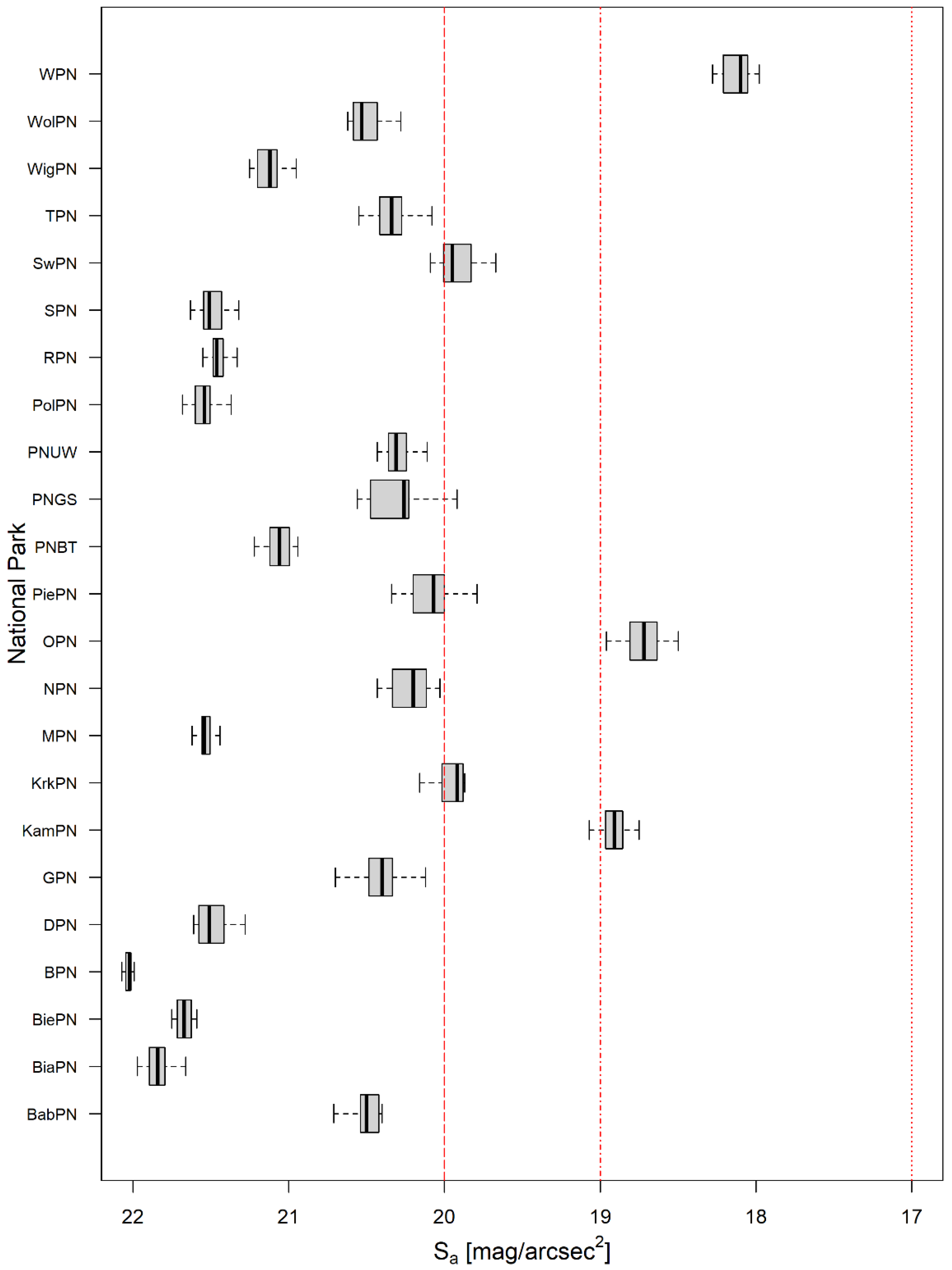
3.2.2. Brightness of Cloudless and Overcast Sky in Landscape Parks

The brightness of the cloudless sky in seven landscape parks (5.6%) was high enough to be in the zone of noticeable ecological influence (Figure A7). These included: Bielańsko-Tyniecki Landscape Park (BTPK), Chojnowski LP (ChojPK), LP Wzniesień Łódzkich (PKWL), Tenczyński LP (TenPK) and Trójmiejski LP (TrojPK), and partially Mazowiecki LP (MPKCL) and LP Dolinki Krakowskie (PKDK). All of them are located in the vicinity of the largest Polish agglomerations: Kraków (BTPK, TenPK, PKDK), Łódź (PKWL), Trójmiasto (TrojPK) and Warszawa (ChojPK, MPKCL). The remaining parks (94.4%) showed no impact of LP on ecosystems, with 16.8% of the parks having an average S_a value exceeding 21.5 mpsas.

Considering the impact of clouds, 16 landscape parks (12.8%) were in the zone of apparent ecological influence (ELP-B) (Figure A8). In addition to the parks that we put in the ELP-C class as a results of the cloudless sky analysis, the following should be included in the ELP-B class: Książański LP (KsPK), the LP Cysterskich Kompozycji Krajobrazowych Rud Wielkich (PKCKKRW), the LP Dolina Bystrzycy (PKDBys), Rogaliński LP (RogPK), Rudawski LP (RudPK), Szczeciński LP “Puszcza Bukowa” (SPKPB), and partially Chęcińsko-Kielecki LP (CKPK), the LP Beskidu Małego (PKBM) and Landscape Park Góry Św. Anny (PKGSA). All of them are located in or near large agglomerations and cities. Another 36 landscape parks (29%) were in the zone of noticeable ecological impact (ELP-C). These results mean that as many as 41.8% of Polish landscape parks are exposed to the effects of light pollution on their ecosystems. On the other hand, significantly more than half of the parks were in the ELP-D group. Only in two parks (1.6%), Ciśniańsko-Wetliński LP and LP Doliny Sanu, the surface brightness of the night sky was close to natural. Both parks are in the buffer zone of Bieszczadzki NP. Including buffers did not introduce any significant changes in the presented analysis.

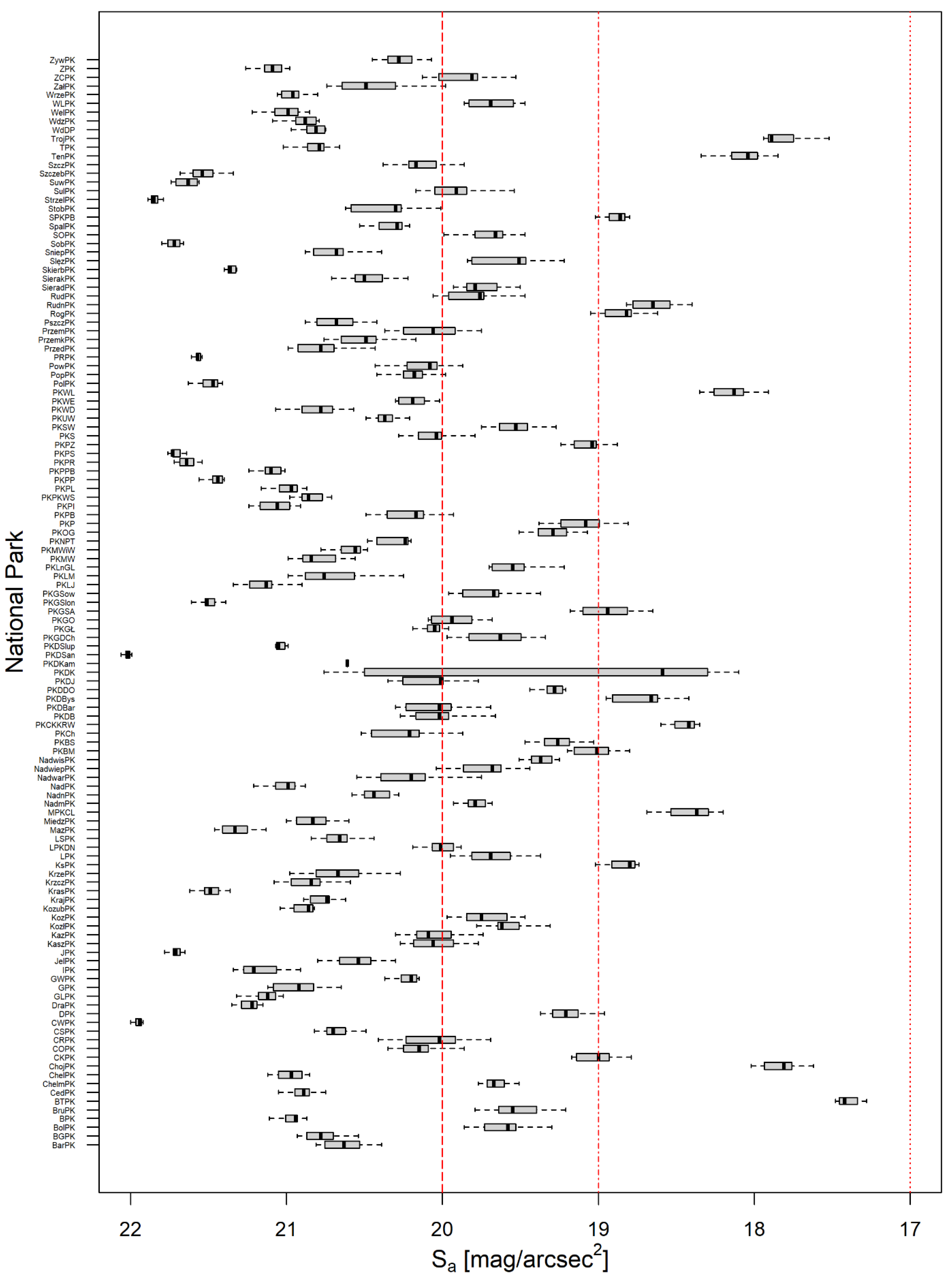
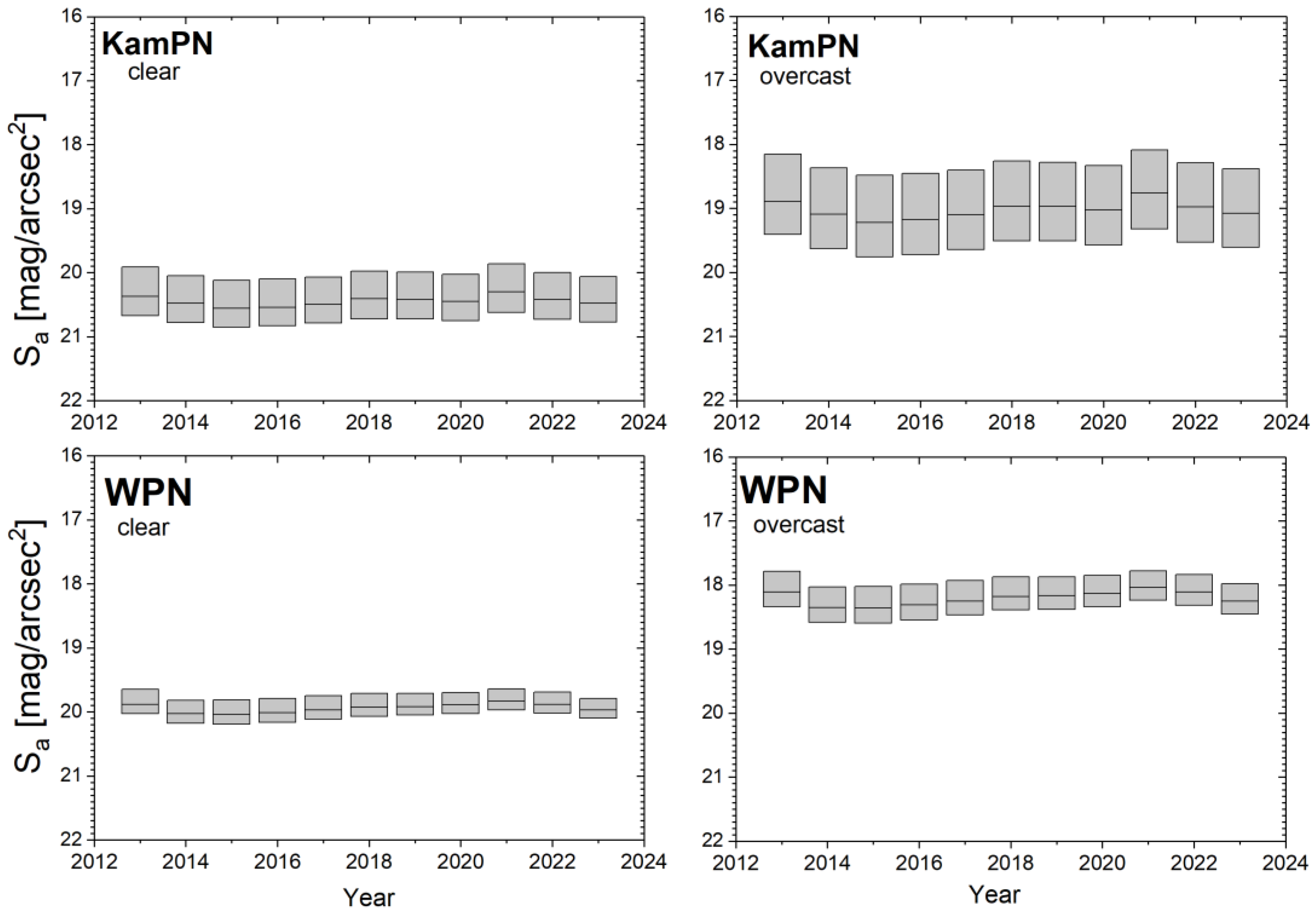
3.2.3. Changes in S_a Values in National and Landscape Parks in 2012–2023

In all analysed national parks, changes in the average value of S_a (night sky brightness) were similar to changes in the average radiance value. After relatively high values for 2013, there was an apparent decrease in the following two years, followed by an equally clear increase and a halt in the trend in 2018–2019. After the pandemic year of 2020, there was a record year in terms of the surface brightness of the sky in 2021, and an apparent decrease was noted in the following years (Figure 5). In some parks (e.g., Ojcowski NP and LP Dolinki Krakowskie, Figure 6), this pattern, especially for the decrease in 2023, was even more pronounced, regardless of whether the data were analysed for a cloudless or cloudy sky, which can probably be associated with the economical switching off of public lighting at night.

4. Discussion and Conclusions

The obtained results indicate that a significant part of the analysed protected areas in Poland, particularly landscape parks, are influenced by LP, consistent with global trends indicating that protected areas are increasingly polluted by artificial light [73]. In our study, introducing the ELP indicator allowed a quantitative assessment of this phenomenon and its translation into potential ecological impacts, which has not been widely practised in Poland so far. In light of the research conducted so far, our results confirm the general trend of increasing potential threats to protected areas generated by nearby urban agglomerations. Early analyses [30,31] showed that many protected areas in the world are within the range of artificial sky glow, even if they emit little or no light. In Poland, this problem was first described in the report “Light Pollution in Poland—2023” [35]. Still, this work significantly extends those findings by also considering landscape parks and classifying their potential threat level using the ELP scale.

Our results demonstrate that effectively conserving biodiversity-rich areas against anthropogenic pressures must also account for ALAN, which propagates over considerable distances as skyglow. Given the still limited public awareness of this phenomenon, it is essential to emphasise that ecosystems are threatened not only by direct light sources, such as street lighting, but also by distant sources located many kilometres away. Moreover, our approach identifies specific ALAN thresholds that pose risks to particular animal groups, providing a strong basis for informed discussions on protecting vulnerable habitats.

The study results indicate that 38.5% of the studied parks, and the potential impact of urban artificial skyglow on their ecosystems was noted, including 22% of national parks and as many as 41.8% of landscape parks. During cloudless nights, these numbers are significantly lower and amount to 6.1% for all parks, including 4.3% for national parks and 6.4% for landscape parks. It should be emphasised, however, that completely cloudless nights are sporadic in Poland [66]. Similarly to the studies by Aubrecht et al. (2010) [30], our analyses also include a buffer that does not significantly change the results, which shows that the administrative boundaries of cities are not a sufficient protection against the influence of LP from urban glow. In turn, the fact that S_a values in some parks (e.g., Bieszczadzki NP) were higher under cloudy conditions than under cloudless conditions confirms the minimal influence of urban glow in such conditions in the most peripheral areas, which may be a reference pattern for the darkest protected areas.

The results are also confirmed by more recent studies, conducted by, among others, Sung [32] and Ji et al. [33], indicating an exceptionally high level of light pollution in parks located near large cities. The examples of the Wielkopolski PN or Bielańsko-Tyniecki PK, which reached S_a values close to the limit of substantial ecological impact (ELP-A), are consistent with the conclusions from studies conducted, for example, in the area of large Korean or Chinese cities.

Considering the discrepancies resulting from the analysis of data provided by VIIRS and the actual increase in the brightness of the night sky [1], the results presented in this article should be treated as an optimistic version, in particular not considering the direct influence of ALAN sources located close to or within the park, as well as the extra-zenithal brightening of the night sky. The number of areas affected by ALAN (ELP-B and ELP-C, and possibly also ELP-A) may be greater. The same caution should be applied to the presented data on changes in the surface brightness of the night sky in 2012–2023, especially the significant decrease in 2023. The reasons may be the following: (a) the energy crisis, rising energy prices and the resulting savings of local government units, and consequently switching off some outdoor lighting during the hours from which VIIRS data can be obtained; (b) replacing traditional lighting with LEDs, and thus an apparent decrease in radiance due to limitations in the spectral range of the VIIRS device; and (c) a combination of factors listed in points a and b. Due to the lack of sufficient field studies, it is impossible to indicate which of the above options is correct for each of the parks studied. This issue will be the subject of further research.

Whether we accept the optimistic or pessimistic option regarding the results of measurements of the surface brightness of the night sky over the studied areas, at least 38.5% of them have ecosystems affected by the adverse effects of light pollution from artificial skyglow. This is a worrying result that requires urgent steps to minimise the impact of this phenomenon. The ELP scale can be a valuable tool for management practice, both in monitoring trends, setting protection priorities, and shaping spatial policies. Of particular importance are the possibilities of its application in the creation of local spatial development plans, environmental impact assessments, and the implementation of dark sky protection zones, which are already being successfully implemented in dark sky parks and biosphere reserves around the world. To sum up, among the actions that could effectively help implement the desired solutions in the areas bordering the parks are:

(a)

introduction of mandatory regulations regarding technical aspects of outdoor lighting, including limiting light intensity at night (or temporarily switching it off), applying a lighting efficiency factor of ULOR = 0%, and using a warmer light colour in light fittings;

(b)

targeted monitoring of the phenomenon, especially of organisms susceptible to ALAN;

(c)

regular measurements of the radiance and surface brightness of the night sky and analysis of light pollution trends;

(d)

considering the negative impact of urban artificial skyglow on the spatial development plans of local government units;

(e)

increasing public awareness of the threat of light pollution;

(f)

promotion of astrotourism, including dark-sky tourism and ecotourism based on the values of nocturnal fauna, which is in line with the assumptions of sustainable tourism;

(g)

formal protection of the night landscape;

(h)

educational and training programmes to disseminate knowledge about the causes and consequences of light pollution and the mechanisms and methods of reducing it.

Implementing the activities mentioned above can be relatively simple using, for example, benchmarking tools, i.e., based on proven solutions that successfully operate in leading places in the world in this respect. National parks and landscape parks that emit significant amounts of artificial light into the sky could implement mechanisms operating in dark sky parks and reserves, of which there are currently almost three hundred worldwide [74]. In turn, localities emitting a glow of light located in the vicinity of protected areas, and at least peripheral districts of large cities, could introduce optimal solutions known from other local government units, i.e., dark sky communities, of which there are about 70 worldwide, including a dozen or so in Europe [74].

The conclusions from our analysis also suggest the need to extend field studies, among other things, by comparing S_a values with spectrometric measurements and direct observations of the behaviour of selected groups of organisms. This approach, based on correlation with the biological activity of different groups of animals, which we adopted when constructing ELP thresholds, distinguishes this study from previous approaches based mainly on radiometric and model data.

Despite the comprehensive nature of the analysis, this study has several significant limitations that should be considered when interpreting the results. First, the ELP (Ecological Light Pollution) scale refers only to the impact of skyglow. It does not include other forms of light pollution, such as glare or light trespass from infrastructure located inside protected areas. Meanwhile, sources such as street lights, tourist facilities, and others can significantly affect ecosystems at night. Second, although the ELP classification was based on the ecological responses of selected organisms to natural brightness thresholds, it does not consider all species’ specific habitat characteristics and sensitivity. Although useful in a nationwide assessment, such an average may be too simplistic in a global or local context, especially in habitats with high biodiversity. Third, the analysis omitted buffer zones of national parks, although formally aimed at limiting the impact of human activity. This may lead to underestimating threats in these transition zones, where urbanisation pressure is often the greatest.

These limitations indicate the need to supplement the analyses with field measurement studies, multispectral monitoring (especially in the field of LED emissions), and more detailed ecological studies, which will allow for further improvement of the ELP scale and its practical use in nature conservation management.

References

1. Kyba, C.C.M.; Altintas, Y.O.; Walker, C.E.; Newhouse, M. Citizen scientists report global rapid reductions in the visibility of stars from 2011 to 2022. Science 2023, 379, 265–268. [Google Scholar] [CrossRef] [PubMed]
2. Falchi, F.; Cinzano, P.; Duriscoe, D.; Kyba, C.C.M.; Elvidge, C.D.; Baugh, K.; Portnov, B.A.; Rybnikova, N.A.; Furgoni, R. The new world atlas of artificial night sky brightness. Sci. Adv. 2016, 2, e1600377. [Google Scholar] [CrossRef] [PubMed]
3. What is Light Pollution? Available online: https://darksky.org/resources/what-is-light-pollution/ (accessed on 20 December 2024).
4. Obayashi, Y.Y.; Shinobu, T.; Norio, K.; Keigo, S. Indoor light pollution and progression of carotid atherosclerosis: A longitudinal study of the HEIJO-KYO cohort. Environ. Int. 2019, 133, 105184. [Google Scholar] [CrossRef]
5. Xu, Y.X.; Zhang, J.H.; Tao, F.B.; Sun, Y. Association between exposure to light at night (LAN) and sleep problems: A systematic review and meta-analysis of observational studies. Sci. Total Environ. 2023, 857, 159303. [Google Scholar] [CrossRef]
6. Cinzano, P.; Falchi, F.; Elvidge, C.D. The first world atlas of the artificial night sky brightness. Mon. Not. R. Astron. Soc. 2001, 328, 689–707. [Google Scholar] [CrossRef]
7. Longcore, T.; Rich, C. Ecological light pollution. Front. Ecol. Environ. 2004, 2, 191–198. [Google Scholar] [CrossRef]
8. Wallner, S.; Kocifaj, M. Aerosol impact on light pollution in cities and their environment. J. Environ. Manag. 2023, 335, 117534. [Google Scholar] [CrossRef]
9. Liu, M.; Li, W.; Zhang, B.; Hao, Q.; Guo, X.; Liu, Y. Research on the influence of weather conditions on urban night light environment. Sustain. Cities Soc. 2020, 54, 101980. [Google Scholar] [CrossRef]
10. Gaston, K.J.; Ackermann, S.; Bennie, J.; Cox, D.T.C.; Phillips, B.B.; Sánchez de Miguel, A.; Sanders, D. Pervasiveness of biological impacts of artificial light at night. Integr. Comp. Biol. 2021, 61, 1098–1110. [Google Scholar] [CrossRef]
11. Seymoure, B.M.; Buxton, R.; White, J.M.; Linares, C.R.; Fristrup, K.; Crooks, K.; Wittemyer, G.; Angeloni, L. Global artificial light masks biologically important light cycles of animals. Front. Ecol. Environ. 2025, 23, e2832. [Google Scholar] [CrossRef]
12. Garrett, J.; Donald, P.; Gaston, K. Skyglow extends into the world’s key biodiversity areas. Anim. Conserv. 2019, 23, 153–159. [Google Scholar] [CrossRef]
13. Evens, R.; Lathouwers, M.; Pradervand, J.; Jechow, A.; Kyba, C.C.M.; Shatwell, T.; Jacot, A.; Ulenaers, E.; Kempenaers, B.; Eens, M. Skyglow relieves a crepuscular bird from visual constraints on being active. Sci. Total Environ. 2023, 900, 165760. [Google Scholar] [CrossRef]
14. Creemers, J.; Eens, M.; Ulenaers, E.; Lathouwers, M.; Evens, R. Skyglow facilitates prey detection in a crepuscular insectivore: Distant light sources create bright skies. Environ. Pollut. 2025, 369, 125821. [Google Scholar] [CrossRef]
15. Kupprat, F.; Hölker, F.; Kloas, W. Can skyglow reduce nocturnal melatonin concentrations in Eurasian perch? Environ. Pollut. 2020, 262, 114324. [Google Scholar] [CrossRef]
16. Hirt, M.R.; Evans, D.M.; Miller, C.R.; Ryser, R. Light pollution in complex ecological systems. Philos. Trans. R. Soc. B 2023, 378, 20220351. [Google Scholar] [CrossRef]
17. Schreuder, D.A. Light trespass: Causes, remedies and actions. In Proceedings of the CIE/MBE Symposium “Lighting and Signalling for Transport”, Budapest, Hungary, 22–23 September 1986. [Google Scholar]
18. Light Pollution—The Problem of Glare. Available online: https://www.rasc.ca/sites/default/files/LightPollution-TheProblemofGlare.pdf (accessed on 20 December 2024).
19. Chepesiuk, R. Missing the dark: Health effects of light pollution. Environ. Health Perspect. 2009, 117, A20–A27. [Google Scholar] [CrossRef]
20. Gaston, K.J.; Visser, M.E.; Hölker, F. The biological impacts of artificial light at night: The research challenge. Philos. Trans. R. Soc. B 2015, 370, 20140133. [Google Scholar] [CrossRef]
21. Cao, M.; Xu, T.; Yin, D. Understanding light pollution: Recent advances on its health threats and regulations. J. Environ. Sci. 2022, 127, 589–602. [Google Scholar] [CrossRef]
22. Bożejko, M.; Tarski, I.; Małodobra-Mazur, M. Outdoor artificial light at night and human health: A review of epidemiological studies. Environ. Res. 2023, 218, 115049. [Google Scholar] [CrossRef]
23. Hölker, F.; Wolter, C.; Perkin, E.K.; Tockner, K. Light pollution as a biodiversity threat. Trends Ecol. Evol. 2010, 25, 681–682. [Google Scholar] [CrossRef]
24. Falcón, J.; Torriglia, A.; Attia, D.; Viénot, F.; Gronfier, C.; Behar-Cohen, F.; Martinsons, C.; Hicks, D. Exposure to Artificial Light at Night and the Consequences for Flora, Fauna, and Ecosystems. Front. Neurosci. 2020, 14, 602796. [Google Scholar] [CrossRef] [PubMed]
25. Owens, A.C.S.; Lewis, S.M. The impact of artificial light at night on nocturnal insects: A review and synthesis. Ecol. Evol. 2018, 8, 11337–11358. [Google Scholar] [CrossRef] [PubMed]
26. Adams, C.A.; Fernández-Juricic, E.; Bayne, E.M.; St. Clair, C.C. Effects of artificial light on bird movement and distribution: A systematic map. Environ. Evid. 2021, 10, 37. [Google Scholar] [CrossRef]
27. Stone, E.L.; Harris, S.; Jones, G. Impacts of artificial lighting on bats: A review of challenges and solutions. Mamm. Biol. 2015, 80, 213–219. [Google Scholar] [CrossRef]
28. Vandersteen, J.; Kark, S.; Sorrell, K.; Levin, N. Quantifying the impact of light pollution on sea turtle nesting using ground-based imagery. Remote Sens. 2020, 12, 1785. [Google Scholar] [CrossRef]
29. Bennie, J.; Davies, T.W.; Cruse, D.; Gaston, K.J. Ecological effects of artificial light at night on wild plants. J. Ecol. 2016, 104, 611–620. [Google Scholar] [CrossRef]
30. Aubrecht, C.; Jaiteh, M.; Sherbinin, A. Global Assessment of Light Pollution Impact on Protected Areas. Available online: https://ciesin.climate.columbia.edu/sites/ciesin.climate.columbia.edu/files/content/light-pollution-Jan2010.cleaned.pdf (accessed on 13 May 2025).
31. Gaston, K.J.; Duffy, J.P.; Bennie, J. Quantifying the erosion of natural darkness in the global protected area system. Conserv. Biol. 2015, 29, 1132–1141. [Google Scholar] [CrossRef]
32. Sung, C.Y. Light pollution as an ecological edge effect: Landscape ecological analysis of light pollution in protected areas in Korea. J. Nat. Conserv. 2022, 66, 126148. [Google Scholar] [CrossRef]
33. Ji, M.; Xu, Y.; Yan, Y.; Zhu, S. Evaluation of the light pollution in the nature reserves of China based on NPP/VIIRS nighttime light data. Int. J. Digit. Earth 2024, 17, 2347442. [Google Scholar] [CrossRef]
34. Kurt, Z.; Aksaker, N.; Yerli, S.K.; Erdoğan, M.K. Investigating potential Dark Sky Parks in Balkans. Astrophys. Space Sci. 2024, 369, 84. [Google Scholar] [CrossRef]
35. Kotarba, A.Z. (Ed.) Light Pollution in Poland. Report 2023; Centrum Badań Kosmicznych PAN: Warsaw, Poland, 2023. (In Polish) [Google Scholar]
36. Dz.U. 2004 nr 92 poz. 880. Ustawa z Dnia 16 Kwietnia 2004 r. o Ochronie Przyrody. Available online: https://isap.sejm.gov.pl/isap.nsf/DocDetails.xsp?id=wdu20040920880 (accessed on 13 May 2025).
37. Formy Ochrony Przyrody. Available online: https://www.gov.pl/web/gdos/formy-ochrony-przyrody (accessed on 21 December 2024).
38. Kruczek, Z. Frekwencja w Atrakcjach Turystycznych w Roku 2020; Polska Organizacja Turystyczna: Warsaw, Poland, 2021. [Google Scholar]
39. Rąkowski, G. Parki Narodowe w Polsce; Instytut Ochrony Środowiska: Warsaw, Poland, 2002. [Google Scholar]
40. Rąkowski, G.; Smogorzewska, M.; Janczewska, A.; Wójcik, J.; Walczak, M.; Pisarski, Z. Parki Krajobrazowe w Polsce; Instytut Ochrony Środowiska: Warsaw, Poland, 2004. [Google Scholar]
41. Palomo, I.; Martín-López, B.; Potschin, M.; Haines-Young, R.; Montes, C. National parks, buffer zones and surrounding lands: Mapping ecosystem service flows. Ecosyst. Serv. 2013, 4, 104–116. [Google Scholar] [CrossRef]
42. Ściężor, T.; Czaplicka, A.; Czaplicka, Z. Light pollution in the Tatra National Park. Arch. Environ. Prot. 2024, 50, 22–30. [Google Scholar] [CrossRef]
43. Iwanicki, G. The level of light pollution in Polish national parks. In Różnorodnie o Bioróżnorodności; Terlecka, M.K., Ed.; Wydawnictwo Armagraf: Krosno, Poland, 2014; pp. 31–40. (In Polish) [Google Scholar]
44. Kosai, H.; Isobe, S. Organised observations of night-sky brightness in Japan during 1987–1989. Publ. Astron. Soc. Aust. 1991, 9, 180–183. [Google Scholar] [CrossRef]
45. Cinzano, P.; Falchi, F.; Elvidge, C.D. Naked eye star visibility and limiting magnitude mapped from DMSP-OLS satellite data. Mon. Not. R. Astron. Soc. 2001, 323, 34–46. [Google Scholar] [CrossRef]
46. Berry, R.L. Light pollution in Southern Ontario. J. R. Astron. Soc. Can. 1976, 70, 97–115. [Google Scholar]
47. Bortle, J.E. Introducing the Bortle Dark-Sky Scale. Sky Telesc. 2001, 101, 126–129. [Google Scholar]
48. Da Silva, A.; Kempenaers, B. Singing from North to South: Latitudinal variation in timing of dawn singing under natural and artificial light conditions. J. Anim. Ecol. 2017, 86, 1286–1297. [Google Scholar] [CrossRef]
49. Bruni, A.; Mennill, D.J.; Foote, J.R. Dawn chorus start time variation in a temperate bird community: Relationships with seasonality, weather, and ambient light. J. Ornithol. 2014, 155, 877–890. [Google Scholar] [CrossRef]
50. Da Silva, A.; Samplonius, J.M.; Schlicht, E.; Valcu, M.; Kempenaers, B. Artificial night lighting rather than traffic noise affects the daily timing of dawn and dusk singing in common European songbirds. Behav. Ecol. 2014, 25, 1037–1047. [Google Scholar] [CrossRef]
51. Miller, M.W. Apparent effects of light pollution on singing behavior of American robins. Condor 2006, 108, 130–139. [Google Scholar] [CrossRef]
52. Catto, C.M.; Racey, P.A.; Stephenson, P.J. Activity patterns of the serotine bat (Eptesicus serotinus) at a roost in southern England. J. Zool. 1995, 235, 635–644. [Google Scholar] [CrossRef]
53. Voigt, C.C.; Dekker, J.; Fritze, M.; Gazaryan, S.; Hölker, F.; Jones, F.; Lewanzik, D.; Limpens, H.; Mathews, F.; Rydell, J.; et al. The impact of light pollution on bats varies according to foraging guild and habitat context. BioScience 2021, 71, 1103–1109. [Google Scholar] [CrossRef]
54. Kawahara, A.Y.; Plotkin, D.; Hamilton, C.A.; Gough, H.; St Laurent, R.; Owens, H.L.; Homziak, N.T.; Barber, J.R. Diel behavior in moths and butterflies: A synthesis of data illuminates the evolution of temporal activity. Org. Divers. Evol. 2018, 18, 13–27. [Google Scholar] [CrossRef]
55. Wong, L.M.K.; Didham, R.K. Global meta-analysis reveals overall higher nocturnal than diurnal activity in insect communities. Nat. Commun. 2024, 15, 3236. [Google Scholar] [CrossRef]
56. Williams, C.B. The times of activity of certain nocturnal insects, chiefly Lepidoptera, as indicated by a light-trap. Trans. R. Entomol. Soc. Lond. 2009, 83, 523–556. [Google Scholar] [CrossRef]
57. Owens, C.S.; Cochard, P.; Durrant, J.; Farnworth, B.; Perkin, E.K.; Seymoure, B. Light pollution is a driver of insect declines. Biol. Conserv. 2020, 241, 108259. [Google Scholar] [CrossRef]
58. Cresswell, W.; Harris, S. The effects of weather conditions on the movements and activity of badgers (Meles meles) in a suburban environment. J. Zool. 1988, 216, 187–194. [Google Scholar] [CrossRef]
59. Wise, S. Studying the ecological impacts of light pollution on wildlife: Amphibians as models. In Starlight: A Common Heritage; UNESCO—MaB: Paris, France, 2014; pp. 107–116. [Google Scholar]
60. Grubisic, M. Waters under artificial lights: Does light pollution matter for aquatic primary producers? Bull. Limnol. Oceanogr. 2018, 27, 76–81. [Google Scholar] [CrossRef]
61. Thomas, R.J.; Cuthill, I.C.; Goldsmith, A.R.; Cosgrove, D.F.; Lidgate, H.C.; Burdett Proctor, S.L. The trade-off between singing and mass gain in a daytime-singing bird, the European Robin. Behaviour 2003, 140, 387–404. [Google Scholar] [CrossRef]
62. Cuthill, I.C.; MacDonald, W.A. Experimental manipulation of the dawn and dusk chorus in the blackbird Turdus merula. Behav. Ecol. Sociobiol. 1990, 26, 209–216. [Google Scholar] [CrossRef]
63. Jechow, A.; Hölker, F. Snowglow—The amplification of skyglow by snow and clouds can exceed full moon illuminance in suburban areas. J. Imaging 2019, 5, 69. [Google Scholar] [CrossRef] [PubMed]
64. Kyba, C.C.; Ruhtz, T.; Fischer, J.; Hölker, F. Cloud coverage acts as an amplifier for ecological light pollution in urban ecosystems. PLoS ONE 2011, 6, e17307. [Google Scholar] [CrossRef]
65. Ribas, S.J.; Torra, J.; Figueras, F.; Paricio, S.; Canal-Domingo, R. Amplification (or not) of light pollution due to the presence of clouds. In Highlights on Spanish Astrophysics IX; Cambridge University Press: Cambridge, UK, 2017; pp. 754–759. [Google Scholar]
66. Tomczyk, A.M.; Bednorz, E. (Eds.) Atlas klimatu Polski (1991–2020); Bogucki Wydawnictwo Naukowe: Poznań, Poland, 2022. (In Polish) [Google Scholar]
67. Ściężor, T. Naturalne i Antropogeniczne Czynniki Łuny Świetlnej Nocnego Nieba; Wydawnictwo Politechniki Krakowskiej: Kraków, Poland, 2018. (In Polish) [Google Scholar]
68. Garstang, R.H. Model for artificial night-sky illumination. Publ. Astron. Soc. Pac. 1986, 98, 364–375. [Google Scholar] [CrossRef]
69. U.S. Standard Atmosphere, 1962; ICAO Standard Atmosphere to 20 Kilometers, Proposed ICAO Extension to 32 Kilometers, Tables and Data to 700 Kilometers. U.S. Government Printing Office: Washington, DC, USA, 1962.
70. Román, M.O.; Wang, Z.; Sun, Q.; Kalb, V.; Miller, S.D.; Molthan, A.; Schultz, L.; Bell, J.; Stokes, E.C.; Pandey, B.; et al. NASA’s Black Marble nighttime lights product suite. Remote Sens. Environ. 2018, 210, 113–143. [Google Scholar] [CrossRef]
71. Li, T.; Zhu, Z.; Wang, Z.; Román, M.O.; Kalb, V.L.; Zhao, Y. Continuous monitoring of nighttime light changes based on daily NASA’s Black Marble product suite. Remote Sens. Environ. 2022, 282, 113269. [Google Scholar] [CrossRef]
72. Teikari, P. Light Pollution: Definition, Legislation, Measurement, Modeling and Environmental Effects; Universitat Politècnica de Catalunya: Barcelona, Spain, 2007. [Google Scholar]
73. Guetté, A.; Godet, L.; Juigner, M.; Robin, M. Worldwide increase in artificial light at night around protected areas and within biodiversity hotspots. Biol. Conserv. 2018, 223, 97–103. [Google Scholar] [CrossRef]
74. World List of Dark Sky Places. Available online: https://darksky.org/what-we-do/international-dark-sky-places/all-places/ (accessed on 12 May 2025).
Figure 1. Location of national parks and landscape parks in Poland (park numbers according to Table A1 and Table A2 in Appendix A).
Sustainability 17 04824 g001
Figure 2. Sa values vs. cloud cover, estimated in the field of view of SQM-L, in different research areas (based on: [67]). Numbers correspond accordingly to the measurements made in: large cities (1–3), suburban villages (4–6), mountain villages (7–11) and interior of the mountains (12–14).
Sustainability 17 04824 g002
Figure 3. Changes in the mean annual radiance in 2012–2023 in the areas of Kampinoski National Park (KamPN), Wielkopolski National Park (WPN), Białowieski National Park (BiaPN) and Bieszczadzki National Park (BPN).
Sustainability 17 04824 g003
Figure 4. Changes in the mean annual radiance in 2012–2023 from the area of Bielańsko-Tyniecki LP (BTPK), Trójmiejski LP (TrojPK), Krasnobrodzki LP (KrasPK) and Stobrawski LP (StobPK).
Sustainability 17 04824 g004
Figure 5. Changes in the Sa value of cloudless and cloudy sky in 2012–2023 in the Kampinoski National Park and Wielkopolski National Park.
Sustainability 17 04824 g005
Figure 6. Changes in the Sa value for a cloudless (left) and overcast sky (right) in 2012–2023 in Ojcowski National Park (OPN) and Landscape Park Dolinki Krakowskie (PKDK).
Sustainability 17 04824 g006
Disclaimer/Publisher’s Note: The statements, opinions and data contained in all publications are solely those of the individual author(s) and contributor(s) and not of MDPI and/or the editor(s). MDPI and/or the editor(s) disclaim responsibility for any injury to people or property resulting from any ideas, methods, instructions or products referred to in the content.