Article

Evolution Characteristics and Influencing Factors of Agricultural Drought Resilience: A New Method Based on Convolutional Neural Networks Combined with Ridge Regression

1
State Key Laboratory of Hydroscience and Engineering, Tsinghua University, Beijing 100084, China
2
School of Water Conservancy & Civil Engineering, Northeast Agricultural University, Harbin 150030, China
3
Joint International Research Laboratory of Habitat Health of Black Soil in Cold Regions, Ministry of Education, Northeast Agricultural University, Harbin 150030, China
4
Key Laboratory of Effective Utilization of Agricultural Water Resources of Ministry of Agriculture and Rural Affairs, Northeast Agricultural University, Harbin 150030, China
5
Heilongjiang Provincial Key Laboratory of Water Resources and Water Conservancy Engineering in Cold Region, Northeast Agricultural University, Harbin 150030, China
6
Research Center for Eco-Environment Protection of Songhua River Basin, Northeast Agricultural University, Harbin 150030, China
*
Author to whom correspondence should be addressed.
These authors contributed equally to this work.
Sustainability 2025, 17(11), 4808; https://doi.org/10.3390/su17114808
Submission received: 24 March 2025 / Revised: 7 May 2025 / Accepted: 21 May 2025 / Published: 23 May 2025
(This article belongs to the Special Issue Climate-Driven Droughts: Pathways to Resilience in Line with SDG13)

Abstract

:
To enhance the precision of regional agricultural drought resilience evaluation, a convolutional neural network optimized with Adam with weight decay (AdamW–CNN) was constructed. Based on local agricultural economic development regulations and utilizing the Driving Force–Pressure–State–Impact–Response (DPSIR) conceptual model, sixteen indicators of agricultural drought resilience were selected. Subsequently, data preprocessing was conducted for Qiqihar City, Heilongjiang Province, China, which encompasses an area of 42,400 km2. The drought resilience was accurately assessed based on the developed AdamW–CNN model from 2000 to 2021 in the study area. The key driving factors behind the spatiotemporal evolution of drought resilience were identified using gray relational analysis, and the future evolution trend of agricultural drought resilience was revealed through Ridge regression analysis improved by the Kepler optimization algorithm (KOA–Ridge). The results indicated that the agricultural drought resilience in Qiqihar City exhibited a trend of initial fluctuations, followed by a significant increase in the middle phase, and then stable development in the later stage. Precipitation, investment in the primary industry, grain output per unit of cultivated area, per capita cultivated land area, and the proportion of effective irrigation area were the primary driving factors in the study area. By simulating the drought resilience index of four typical regions and analyzing its evolution, it was found that the AdamW–CNN model, combined with the KOA–Ridge model, has greater advantages over the RMSProp-CNN model and the CNN model in terms of fit, stability, reliability, and evaluation accuracy. These findings provide a robust model for measuring agricultural drought resilience, offering valuable insights for regional drought prevention and management.

1. Introduction

In recent years, drought has posed an increasingly serious threat to regional sustainable development and human society [1]. On 19 June 2017, the UN Food and Agriculture Organization presented at the International Symposium on Drought in Rome: the area of land affected by drought has doubled since the 1970s, and the frequency of droughts is increasing globally [2]. In the context of global warming, the uncertainty of drought occurrence will further increase, and different geographical and climatic conditions will lead to different drought patterns and postdisaster recovery methods; thus, the resulting losses and impacts of agricultural drought will become more pronounced. For severe agricultural drought, Standardized Precipitation Evapotranspiration Index (SPEI) values below −1.5 are typically associated with significant soil moisture deficits, leading to substantial agricultural impacts, such as reduced crop yields or crop failure. Therefore, there is an urgent need to study agricultural drought in depth and seek efficient strategies.
Most existing studies have focused on a single factor or calculated a drought index to assess agricultural drought risk and analyze its influencing factors. In 1965, the meteorologist Wayne Palmer proposed the Palmer Drought Severity Index (PDSI) on the basis of the relationship between water supply and demand to measure drought conditions [3]. In 1993, McKee T B et al. proposed the Standardized Precipitation Index (SPI), which has attracted widespread attention due to its advantages such as convenient calculation and flexible time measurement [4]. However, it ignores factors such as evapotranspiration, which makes it have certain limitations in drought monitoring. In 2010, Vicente-Serrano S M et al. considered the evapotranspiration factor based on the SPI and proposed the SPEI [5]. This index can effectively reflect the water loss on a long time scale and has strong applicability in drought monitoring in different regions. G Pellicone et al. analyzed the drought situation in Calabria, Italy, by analyzing and calculating the Dematon drought index [6]. Swearingen suggested that, in addition to precipitation, a lack of arable land and population pressure are the main reasons for the increased impact of agricultural drought [7]. There have been few in-depth discussions on agricultural drought resilience and multiangle analysis; since an agricultural drought system is typically complex, response strategies from a single disaster risk perspective are relatively limited. The identification of more scientific and effective assessment theories and methods is urgently needed for agricultural drought prevention, disaster reduction and regional sustainable development. Since Holling et al. introduced the concept of resilience into the field of ecology, many scholars have focused on qualitative and quantitative disaster resilience research [8], which is intuitively expressed as the ability of a system to cope with interference and maintain its original state [9,10]. Agricultural drought resilience refers to the ability of agricultural systems to maintain their basic functions, structures, and productivity through resistance, adaptation, and rapid recovery in the event of drought shocks, and even to achieve a higher level of sustainable development through adjustment. For a complex system, drought resilience reflects three kinds of abilities in the affected body: the ability to withstand drought before it happens; response capacity in the event of drought; and resilience after drought. In the development process, drought resilience has different characteristics and functions throughout and during different periods. The perspective of resilience can provide new ideas for improving regional drought response capacity and formulating disaster reduction strategies. Improving agricultural drought resilience is inextricably linked to the core principles of sustainable agriculture. Its essence lies in achieving multi-dimensional synergy of stabilizing agricultural productivity, improving resource utilization efficiency, maintaining economic sustainability and promoting social equity by enhancing the adaptability and resistance of agricultural systems to drought. In recent years, the study of drought resilience has received extensive attention from international scholars. Gebremedhin et al. found that developing ecosystem services and enhancing soil and water conservation are appropriate strategies to enhance drought resilience through the study of the causes and impacts of resilience [11]. Ram et al. found that economic development is a key factor in the growth of agricultural drought resilience [12]. Ringetani et al. found that a good economic, demographic, and resource base can lead to greater resilience to drought [13].
Because the study of resilience theory in the field of drought is still in its development stage, most researchers have conducted only qualitative or quantitative screenings of indicators in a certain area [14,15,16], which cannot accurately express the correlation between indicators and the rationality of constructing an indicator system. The Driver–Pressure–State–Impact–Response (DPSIR) model is a conceptual framework for analyzing the interaction between environmental and social systems. It is widely used in sustainable development, ecological management, and policy evaluation research. The model can reveal the dynamic relationship between human activities and environmental changes through causal chains. Thus, the DPSIR conceptual model was used to build a drought resilience index system [17], and an overall analysis was carried out by integrating factors such as nature, agriculture, culture, and economy. The model is characterized by a clear framework and hierarchy and is a reliable method for reflecting the response mechanism of drought resilience. Many scholars have conducted in-depth research on the evaluation methods of disaster resilience. Rey et al. investigated drought information in the eastern region of the United Kingdom through online surveys and interviews with farmers and used the results to assess the response capability of different management measures to future droughts [18]. Maity et al. used a Plackett copula function to characterize the vulnerability and resilience of regional drought by analyzing soil moisture [19]. Wang H et al. constructed a “social–economic–environmental–institutional” drought resilience assessment framework [20]. Xu et al. used interpretive structural modeling (ISM) combined with an analytic hierarchy process to evaluate the resilience of three cities in the Yellow River Basin [21]. Ilse Kotzee et al. used principal component analysis (PCA) to evaluate regional flood disaster resilience by selecting and analyzing 24 indicators, assessing the difference in flood resilience between urban interiors and urban edges through spatial analysis [22]. However, there are also some shortcomings: ISM is easily affected by subjective factors, thus affecting the accuracy of evaluation [23]; selecting Copula function parameters is complicated, which makes the confidence interval of the conclusion difficult to estimate [24]; analytic hierarchy process and TOPSIS approaches rely on the subjective judgment of experts, which may lack objectivity in the evaluation results [25,26]; and PCA obtains evaluation results using a few principal components, leading to insufficient comprehensiveness in conclusions [27]. In summary, traditional methods cannot meet the needs of disaster resilience evaluation, so there is an urgent need to find a new evaluation method to assess disaster resilience.
In recent years, research on machine learning has continually improved. However, the limitations of traditional machine learning models such as support vector machines, projection pursuits and extreme learning machines can lead to insufficient credibility in the evaluation results. The projection pursuit evaluation model can easily fall into a local optimal solution when conducting a multi-dimensional index evaluation [28], and the SVM model is inconvenient to use because its kernel function is uncertain [29]. Although the extreme learning machine model can deal with nonlinear problems by introducing a nonlinear activation function, it still has the disadvantage of poor model fitting ability [30]. As deep learning methods continue to evolve, convolutional neural networks (CNNs) occupy an extremely important position in the field of deep learning and are widely used in various fields because of their ability to automatically extract data features. This is especially relevant in the processing of high-dimensional data, and these advantages [31], coupled with fewer weights and biased parameters, offer relatively high stability and generalizability [32,33]. The performance of convolutional neural networks mainly depends on the learning rate. When the learning rate is low, the model will converge for a long time; in contrast, if the learning rate is high, overfitting can occur [34]. Loshchilov and Frank proposed an Adam optimization algorithm based on weight decay (AdamW). By considering the gradient, an additional attenuation term is added to achieve weight regularization [35,36], enabling the automatic adjustment of the learning rate when processing large-scale data and alleviating the shortcomings of the CNN in learning rate selection [32].
There is a progressive and cyclic relationship between DPSIR indicators. When applying CNN to process aggregated time series indicators based on the DPSIR framework, its core advantage is that CNN can automatically capture the coordinated changes of indicator subsets in specific time segments through the local connection weight sharing mechanism. Compared with recursive network models such as LSTMs, CNN is more suitable for extracting indicator features with hierarchical correlation and local temporal causal chains under the DPSIR framework, and is more conducive to avoiding overfitting and maintaining model interpretability in multi-dimensional indicator scenarios. In terms of feature sharing and local connection, CNNs offer excellent big data processing and model generalizability, but they cannot directly calculate the individual weight of each input independent variable, and they cannot predict if the data are incomplete. In view of the difficulty in calculating index weights and the difficulty in forecasting due to incomplete data, gray relational analysis has been used to screen key driving factors. The Kepler optimization algorithm (KOA) has been used to optimize the regularization parameter λ in Ridge regression. Combining the drought resilience index calculated by the proposed CNN optimized by AdamW (AdamW–CNN), a Ridge regression equation optimized by the KOA was constructed, using key driving factors to analyze the future evolution of drought resilience and the driving mechanism and quantitative relationship of the key driving factors of drought resilience. The accurate measurement of drought resilience can provide theoretical support for the prediction of future drought resilience.
The main objectives of this study are as follows:
(1)
Construct a regional agricultural drought resilience evaluation index system based on the DPSIR conceptual model.
(2)
Accurately evaluate the regional agricultural drought resilience characteristics using the AdamW–CNN model.
(3)
Identify the key driving factors of regional agricultural drought resilience, establish the KOA–Ridge regression equation, and analyze the future evolution trend of resilience.
(4)
Verify the performance of AdamW–CNN and KOA–Ridge models.
The structure of this paper is as follows: Firstly, the data of agricultural drought resilience indicators are preprocessed. Secondly, based on the DPSIR conceptual model, the resilience evaluation index system is constructed. Subsequently, the new AdamW–CNN model is used to accurately measure the resilience of agricultural drought in the study area and identify the key drivers of its spatiotemporal evolution. On this basis, an improved Ridge regression model is used to predict the evolution of agricultural drought resilience in the future. Finally, the advancement and applicability of the model are discussed in depth. This strategy of building machine learning models based on multi-dimensional raw data can better reveal the mechanism of agricultural drought resilience. A general flowchart is presented in Figure 1 for a comprehensive understanding of the article.

2. Study Area and Data Source

2.1. Study Area

Qiqihar City, with an area of 42,400 km2, is located in the southwest of Heilongjiang Province and the south of the Songnen Plain, located at 123.55°–126.68° E and 45.27°–48.28° N. In addition to the urban area, it has jurisdiction over 1 county-level city and 8 counties; it is characterized by a temperate continental monsoon climate with four obvious seasons. Dry land is the main planting type, with rich black soil resources. Modern mechanized agricultural production is the main farming activity; according to statistics from meteorological observation data in Qiqihar City, spring rains account for 13–15% of the total annual precipitation. Qiqihar has become the region with the highest temperature, the least precipitation, the strongest winds, and the most evaporation in the province: it is located on the edge of the semiarid zone [37]. Therefore, to ensure orderly agricultural production for the people of Qiqihar, it is necessary to carry out research on drought resilience in Qiqihar City. The specific distribution is shown in Figure 2.

2.2. Data Sources

The Heilongjiang Yearbook (2000–2022), Qiqihar Yearbook (2000–2022), and Qiqihar Economic Statistics Yearbook (2000–2022) were collected from the CNKI. Data for natural, economic, and social indicators in Qiqihar City during the past 22 years were collected and calculated for the study of drought resilience.

3. Methodology

3.1. Analysis of Connotation of Drought Resilience

The concept of resilience comes from the Latin word “resilo”, which means to bounce back. Since Holling [8] introduced the theory of resilience into the field of ecology in 1973, its application in the field of disaster science has been gradually expanded. With extensive research on disaster theory, research on the concept of disaster resilience has increased. Many scholars have defined system resilience. Francis et al. argued that system resilience is the ability of a system to return to a normal state after being disturbed [38]. Liu J et al. believed that system resilience included the ability to influence the disaster factors of a system and the ability to recover after disaster [39]. UNISDR defines resilience as the ability of a system, community, or society to resist, absorb, adapt to, transform, and recover quickly from the effects of danger in a timely and effective manner in the face of danger, and to restore the basic functions of the system through certain management measures [40].
A complex system of agricultural drought resilience reflects three abilities: the ability of agricultural areas to withstand drought before it occurs, the response capacity in the event of a drought, and the resilience of agricultural areas after a drought. In the process of regional agricultural development, agricultural drought resilience has different characteristics and functions throughout and in different periods. Thus, the resilience of agriculture to drought is influenced by many factors. For example, a high forest coverage rate, abundant labor force and abundant agricultural economy can indicate the high resilience of agricultural drought from a certain level, even if agricultural drought resilience is low.

3.2. Index System Construction Method

The DPSIR framework was developed by the European Environment Agency (EEA) in the late 1990s, and it is a conceptual model based on organizational relevance; the goal is to establish a causal chain of driving force, pressure, state, impact, and response [41]. The core philosophy of DPSIR is based on holistic considerations and cannot be separated from any single-factor analysis. The theoretical framework of drought resilience can clearly reflect the theoretical structure through DPSIR; the role of drought resilience and coping strategies at different stages can be clearly reflected from three aspects, before, during, and after the disaster, making the whole framework more three-dimensional, in line with the concept of sustainable development. The drought resilience framework constructed by the DPSIR model is shown in Figure 3.

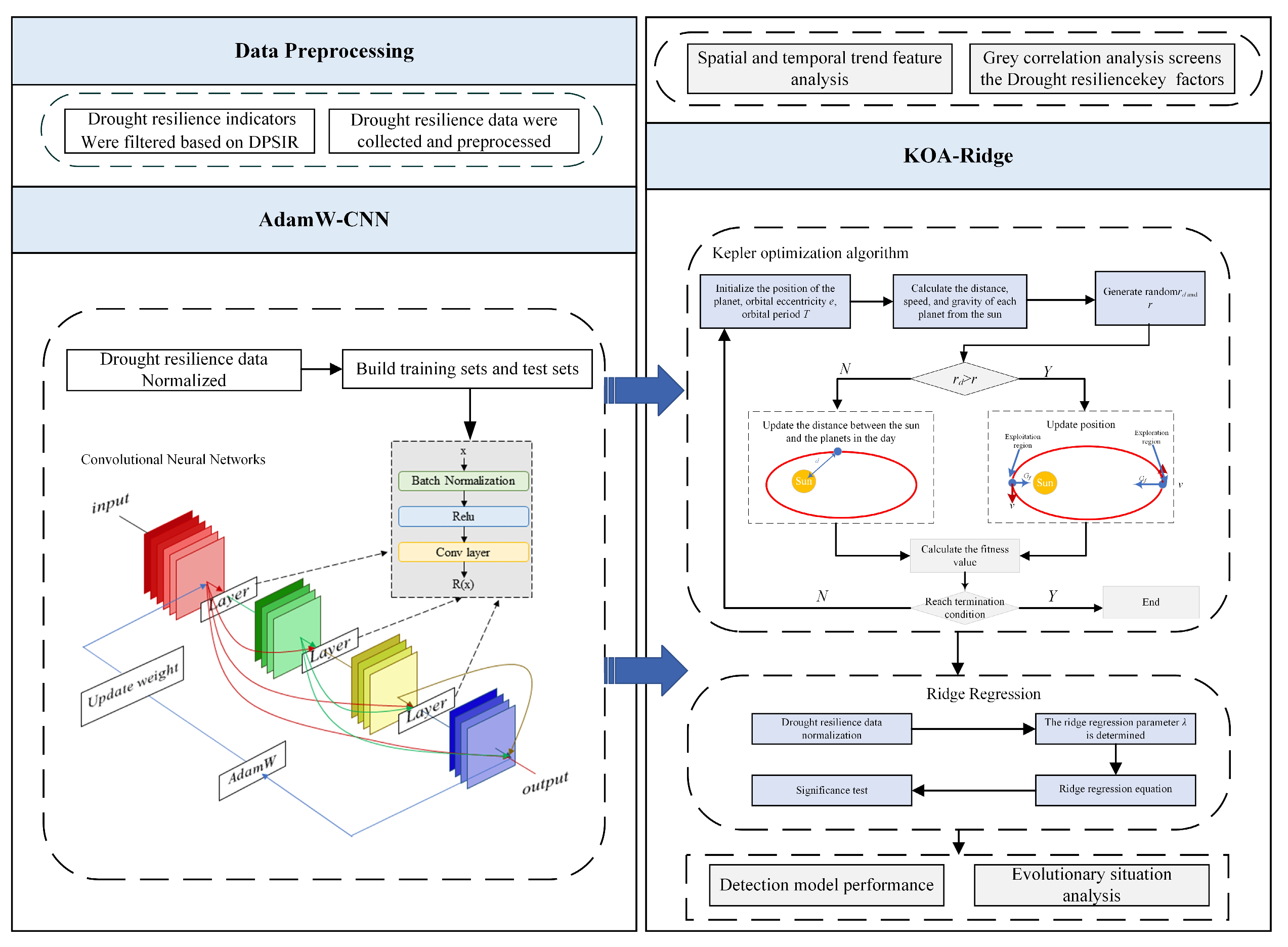
3.3. Data Preprocessing Methods

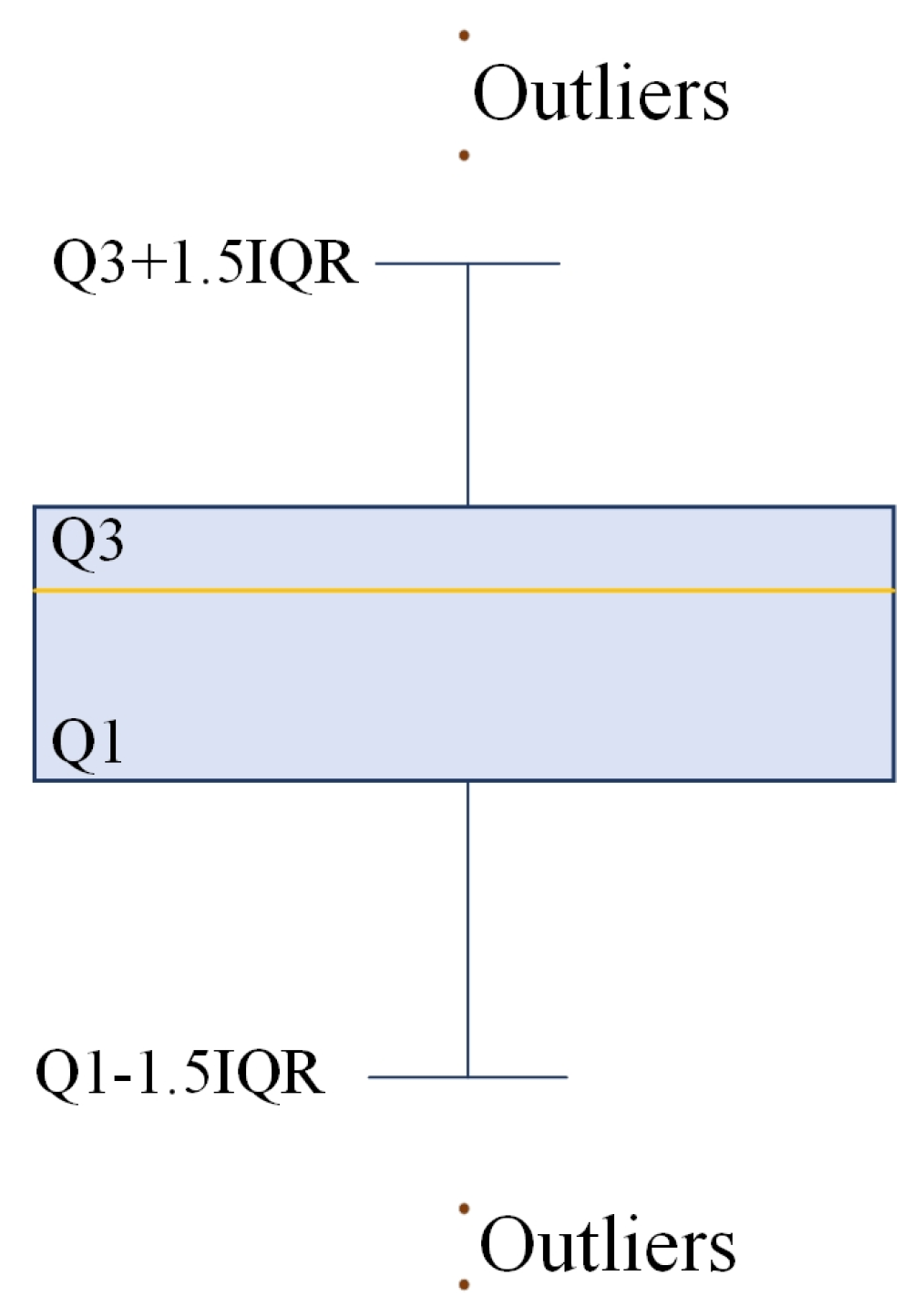
3.3.1. IQR and Boxplot Method

A quartile is a kind of quantile in statistics; that is, all the values are arranged from small to large and divided into four equal parts, and the value at the position of the three dividing points is the quartile [42]. The first quartile (Q1) is 25% of all values in the sample in descending order. The second quartile (Q2) is the median, and the third quartile (Q3) is 75% of all values in the sample ranked from smallest to largest. The difference between Q1 and Q3 is the Interquartile Range (IQR). (Q1 − 1.5IQR) represents the lower bound of the minimum value of the data, and (Q3 + 1.5IQR) represents the upper bound of the maximum value of the data. Outliers represent values greater than Q3 + 1.5IQR and less than Q1 − 1.5IQR. On the basis of this method, a boxplot is used to visualize the IQR method, which makes the processing more intuitive. The process is shown in Figure 4.

3.3.2. Kendall’s Tau-b Correlation Coefficient

Kendall’s Tau-b correlation coefficient is a method for solving correlation proposed by British statistician Maurice Kendall in 1938 [43]; it is suitable for judging the correlation between two columns of discrete ordered data, and its calculation formula is as follows:
τ B = n c n d ( n 0 n 1 ) ( n 0 n 2 )
In the formula, nc is the number of concordant pairs in pair-to-pair comparison, nd is the number of disconcordant pairs in pairings, and n0 is the total logarithm of pairwise comparison, involving the number of invariant x values when n1 is the invariant pair, and the number of invariant y values when n2 is the invariant pair.
In general, τB ≥ 0.80 is a very strong correlation, 0.60 ≤ τB < 0.80 is a strong correlation, 0.40 ≤ τB < 0.60 is a moderate correlation, 0.20 ≤ τB < 0.40 is a weak correlation, and τB < 0.20 is no correlation.

3.4. Model Construction Method

3.4.1. Convolutional Neural Networks

A convolutional neural network is a kind of pre-feedback neural network that includes convolutional computation and has a deep structure, and it is one of the representative algorithms of deep learning [44]. The hyperparameters include learning rate, number of iterations, number of layers, number of neurons per layer, batch size, and weight of each part of the loss function. The hyperparameters involved have their algorithm flow as follows:
(1)
In the convolution layer, the input data is convolved with multiple convolution cores. The mathematical expression of the convolution process is as follows:
( I K ) ( x , y ) = i = a a j = b b I ( x + i , y + j ) K ( i , j )
I is the input image, K is the convolution kernel, (x, y) is the position on the output feature map, and a and b are the half-height and half-width of the convolution kernel, respectively. After each convolutional layer, a nonlinear activation function, such as the ReLU function, is usually applied to increase the nonlinear capability of the network.
(2)
The pooling layer is connected behind the convolutional layer, and its function is to reduce the dimension of the eigenvalues, while maintaining the invariance of the eigenscale to a certain extent. The pooling layer generally only performs dimensionality reduction operations, without parameters and without weight update.
(3)
The input data is propagated alternately through several convolutional layers and pooling layers, and the extracted features are classified by a fully connected layer network. On the fully connected layer, the input is the weighted sum of all the one-dimensional feature vectors expanded by the feature graph and obtained by the activation function. The calculation formula for the fully connected layer is as follows:
y k = f ( w k x k 1 + b k )
In the formula, k is the serial number of the network layer; yk is the output of the fully connected layer; xk−1 is an expanded one-dimensional eigenvector; wk is the weight coefficient; bk is the offset term; and the activation function f uses the Softmax function.
(4)
For specific classification tasks, the CNN needs to minimize the loss function of the network to determine whether the results of the regression model are optimal.

3.4.2. AdamW Adaptive Optimization Algorithm

The AdamW adaptive optimization algorithm is an improved Adam algorithm [45]. Its basic idea is to introduce the idea of weighted attenuation to improve the convergence speed of convolutional neural networks, so as to achieve the purpose of parameter adaptive adjustment. The formula of the AdamW optimization model is as follows:
h t = h t 1 η t α m t v t + ε A d a m w + w h t 1
In the formula,
g t = J t ( h t 1 )
m t = β 1 m t 1 + ( 1 β 1 ) g t
v t = β 2 v t 1 + ( 1 β 2 ) g t 2
m t = m t 1 β 1 t
v t = v t 1 β 2 t
In the formula, learning rate α = 0.01; currently estimated exponential decay rate β1 = 0.9, β2 = 0.999; weight attenuation factor w = 0.01; iteration coefficient ηt = 1; f(h) is the loss function under parameter h; first-order moment momentum mt=0 = 0; second-order moment momentum vt=0 = 0; initialization time step t; iteration parameter ht = 0. To prevent the divisor from being 0, use εAdamW = 10−8.
Equations (6) and (7) are actually weighted averages of the momentum index, while Equations (8) and (9) are bias corrections for mt and vt.

3.4.3. AdamW–CNN Model

The learning rate in CNN determines the degree to which each step of the weight update changes the current weight. Too small a learning rate will lead to a slow updating speed, and too large a learning rate may cross the optimal solution. Therefore, the hyperparameter of the learning rate in the CNN was selected for optimization, and the root mean square error RMSE, mean absolute error MAE, and goodness of Fit R2 of training samples were taken as the objective functions to construct the AdamW–CNN model to achieve iterative optimization of the learning rate and measure drought resilience. The specific steps are as follows:
Step 1: Collect the data training sample set, including input data and output data.
Step 2: Initialize the learning rate of the CNN as 0.001 [46], and determine the attenuation rate of the first moment index β1 as 0.9 and the attenuation rate of the second moment index β2 as 0.999 [35].
Step 3: Determine the fitness function using the root mean square error RMSE, mean absolute error MAE, and goodness of fit R2; its mathematical expression is as follows:
R M S E = 1 m i = 1 m ( y i y i ) 2
M A E = 1 n i = 1 n y ^ i y i
R 2 = 1 i ( y ^ i y i ) 2 i ( y i ¯ y i ) 2
Step 4: Extract the feature O of the convolution layer. The parameters of the convolution layer include the size of the input matrix n, the size of the convolution kernel f, the boundary filling p, and the step size s. The convolution result is rounded down and the calculation formula is as follows:
O = ( n f + 2 p ) / s + 1
Step 5: The pooling layer is generally placed behind the convolutional layer, so the input of the pooling layer is the output of the convolutional layer. Pooling layers reduce the number of parameters, overfitting, and operational complexity by reducing the connections between convolutional layers. After actual operation, it can be seen that the Max pooling method is proven to have a better operation effect. By defining a space neighborhood, the largest element is selected from the modified feature map in the space window.
Step 6: When the output result of the CNN is inconsistent with the expected value, the error is returned layer by layer and the weight is updated. The calculation formula for weight update is as follows:
W n e w = W o l d η L W
In the formula, Wnew is the updated weight, Wold is the current weight, η is the learning rate, and ∂L/∂W is the gradient of the loss function with respect to the weight.
Step 7: Search individual fitness values by calculating the updated learning rate of RMSE, MAE, and R2, and conduct gradient descent to find the current optimal learning rate. Check whether the algorithm meets the termination condition. If yes, go to the next step. If no, repeat Steps 4–6.
Step 8: The tail of the CNN is the fully connected layer, and the regression process is carried out at the end of the entire CNN. The Softmax function is used to extract features for regression analysis.
Step 9: Output the fitness value of the optimal learning rate and the result of regression evaluation.

3.4.4. Gray Relational Analysis

Gray relational analysis (GRA) is a multi-factor statistical analysis method, and its concept was proposed relative to white systems and black systems. The basic principle of its analysis is that the closer the geometric shape of each curve formed by several statistical series, that is, the more parallel the curves, the closer their change trend, and the greater their correlation degree [47]. Therefore, the evaluation objects can be compared and sorted by the correlation degree between each scheme and the optimal scheme. The specific steps are as follows:
Step 1: Determine the analysis sequence and divide the multiple sequences into one parent sequence and several subsequences.
Step 2: Standardize the variables.
Step 3: Let the number of subsequences be m, each sequence has n samples, and the data is as follows:
x m = ( x m ( 1 ) , x m ( 2 ) , , x m ( n ) ) T
Step 4: The formula for the correlation coefficient y is as follows:
y ( x 0 ( n ) , x k ( n ) ) = a + ρ b x 0 ( n ) x k ( n ) + ρ b

3.4.5. Kepler Optimization Algorithm

The Kepler optimization algorithm is compared to the planets and the sun, and the position relationship between them constantly changes with the operation of the algorithm, which is similar to the motion relationship between the planets and the sun in Kepler’s law. The main steps of the KOA are also designed based on this principle [48]. The KOA simulates the behavior process of the algorithm through the process of the planet rotating in an elliptical orbit around the sun to and from perihelion and aphelion. First, the position of the planet representing the decision variable is initialized, and the formula is as follows:
X i j = X i , l o w j + r a n d [ 0 , 1 ] × ( X i , u p j X i , l o w j ) , i = 1 , 2 , , N j = 1 , 2 , , d
In the formula, Xi represents the i-th planet; N represents the number of candidate solutions; d represents the dimension of the optimization problem; Xji,up and Xji,low represent the upper and lower bounds of the j-th decision variable; and rand[0,1] is a random number generated between 0 and 1.
The orbit of the planet around the sun is divided into two processes: near perihelion and near aphelion. The first stage of the process is to reach perihelion by constantly updating the position of the planet. The equation is as follows:
X i ( t + 1 ) = X i ( t ) + σ × v i ( t ) + ( F g i ( t ) + r ) × U × ( X s ( t ) X i ( t ) )
In the formula, X i ( t + 1 ) is the new position of the planet, σ is the velocity direction of the planet, X s ( t ) is the position of the sun, that is, the current position of the best solution, and v i ( t ) is the velocity of the planet at time t, calculated by its distance from the sun, and the closer it is to the sun, the greater the velocity.
The second stage of operation of the KOA is to gradually approach the aphelion, and the position of the planet is constantly updated through Formula (17), so that the position of the planet near the sun is the optimal solution for the number of iterations. The calculation formula is as follows:
X i ( t + 1 ) = X i ( t ) × U 1 + ( 1 U 1 ) × [ X i ( t ) + X s ( t ) + X a ( t ) 3 + h × ( X i ( t ) + X s ( t ) + X a ( t ) 3 X b ( t ) ) ]
In the formula, h is the adaptive factor, and X a ( t ) and X b ( t ) are two random solutions. The KOA will optimize the exploration operator when the planet is away from the sun, and the mining operator when the planet is close to the sun.

3.4.6. KOA–Ridge Regression

Ridge regression is a biased estimator regression method that deals with multicollinearity of independent variables for small-sample data. In contrast to the unbiased estimation of ordinary least squares, its partial regression coefficient is closer to the true value, and the stability and reliability of the model are improved [49]. Based on the linear regression loss function, a regularization term is introduced to increase the weight restriction and reduce the risk of overfitting. Setting the mean squared error MSE as the Ridge regression objective function, the formula is
M S E = 1 n i = 1 n ( y ^ i y i ) 2
In the formula, n is the number of samples, yi is the actual value of the i-th sample, and y i ^ is the predicted value of the i-th sample.
Step 1: Data collected by key driving factors filtered by gray relational analysis was taken as the independent variable xi, and data obtained by CNN regression was taken as the dependent variable, which was denoted as fresilience.
Step 2: The initialization parameter λ is 0.1, and the K-fold cross-validation method is adopted to divide the sample data into 5 equal fractions, in which 1 sample is used as the verification set and 4 samples are used as the training set, and MSE is calculated [50].
Step 3: The parameters of the initialization KOA are set to 100 iterations until the maximum number of iterations is met, and the optimized regularization parameter λ is generated.
Step 4: The final regression calculation equation is generated, and the regression analysis calculation form is as follows:
y = j = 1 n β j x j + w 0
In the formula, n is the number of features, j is the number of features, β is the parameter vector to be learned in Ridge regression, and w0 is the constant term.

3.4.7. Sequence Number Summation Theory

In order to verify the stability and rationality of the evaluation model, the serial number summation theory is adopted to verify it [51,52]. According to the ordinal sum theory, the results obtained by different methods are relatively reasonable. The average and standard deviation of the correlation coefficient of each method are calculated repeatedly, and the method with the highest average correlation coefficient can be considered to be more reasonable than other methods. The specific steps are as follows:
Step 1: Different optimization algorithms are used to systematically evaluate regional drought resilience, and the evaluation results are ranked.
Step 2: Make a relatively reasonable sorting according to the sorting results obtained by different algorithms.
Step 3: Calculate the Spearman rank correlation coefficient between different ranking results and relatively reasonable ranking results.
Step 4: Carry out random sampling and repeat the calculation process of the previous Step 3. After adding the result, the maximum Spearman rank correlation coefficient is the most stable model. Then, the mean and standard deviation of correlation coefficients of each method are calculated many times. The method with the maximum mean and minimum standard deviation has the best rationality and stability. The Spearman rank correlation coefficient formula is as follows:
N = 1 6 × D i 2 n ( n 2 1 )
In the formula, Di represents the difference between the relatively reasonable ranking number of drought resilience of region i and the ranking number of a certain evaluation method. n is the number of regions. N is the rank correlation coefficient, and the closer N is to 1, the greater the correlation between the two ranking results.
The rationality coefficient S and stability coefficient V of the evaluation method are defined as follows:
S = 1 n i = 1 n N i
V = 1 1 n i = 1 n ( N i S ) 2
The AdamW–CNN model and KOA–Ridge Regression model were combined to construct the overall application framework of the model, as shown in Figure 5.

4. Results and Analysis

4.1. Indicator Selection

Based on the DPSIR model, the evaluation framework of drought resilience in the Qiqihar region was constructed from the key factors affecting drought resilience. Indicators were screened based on local actual scenarios and existing research results [18,53].
The natural environment and human influences are the key factors that promote changes in drought resilience; the arable land in Qiqihar is mainly dry land, so the most direct natural environmental influence is precipitation, and population growth rate and density effectively quantify the influence weight of human factors. The most critical pressure carrier in Qiqihar is agricultural production; therefore, the per capita cultivated land area and the proportion of effective irrigation area were selected for study. Under the influence of the objective pressure factors for regional drought, the present situation of nature, agriculture, and human society is exposed, and the forest coverage rate, water resources per capita, grain output per unit cultivated land area, and the proportion of agricultural population are selected for research. The realistic performance of the integrated system of drought resilience has an impact on the stability of drought resilience in Qiqihar City. Therefore, from the two aspects of economic return and agricultural spatial distribution, three indicators of per capita GDP, the proportion of agricultural output and proportion of dry land area were selected for analysis. According to the characteristics of agricultural production in Qiqihar City, four indexes of investment in primary industry, proportion of investment in tertiary industry, number of electromechanical wells per hectare, and total power of agricultural machinery per hectare were selected from the perspectives of social economics and government macro control. Thus, 16 evaluation indicators were selected from the four aspects of nature, agriculture, culture, and economy for the evaluation of drought resilience in Qiqihar. The specific definitions are shown in Table 1.

4.2. Data Preprocessing

To prevent unsmooth outliers in the index dataset from negatively affecting the model evaluation results, the dataset of statistical accounting is adopted. However, under natural conditions, there will be extreme weather events such as hurricanes, heavy rain, and snow. Because this is part of a natural meteorological process, it is not reasonable to estimate these precipitation events and thus not treat them as outliers. The other indicators are identified by the IQR method and boxplot method, and the missing values are identified by K nearest neighbor (KNN) interpolation. The cross-validation method determines the value of K as 6, and the interpolation result is obtained by calculating Formula (1); the result is shown in Figure 6.
Figure 6a shows that the total power of agricultural machinery per hectare, the proportion of investment in the tertiary industry, per capita GDP, and other indicators have more outliers in statistical calculations; after interpolation of the outlier data by the KNN method, Figure 6b shows that all datasets are within the normal range. Therefore, interpolating datasets with fewer missing values and not completely conforming to a normal distribution has a good effect.

4.3. Correlation Test

After the index system is built, a correlation test of different indexes is carried out. Correlation tests help detect multicollinearity between features by identifying whether there are highly correlated features, thus reducing the risk of model overfitting. The results of Kendall’s Tau-b correlation coefficient among all indicators are shown in Figure 7. The blue color in Figure 7 represents negative correlation, the red color represents positive correlation, and the size of the circle represents the strength of the correlation.
Figure 7 shows that there are both positive and negative correlations between the selected indicators, but the overall Kendall Tau-b correlation coefficients are small, ranging from −0.6 to 0.6, indicating that the collinearity between the data is low, which can ensure the high accuracy of the model operation.

4.4. Drought Resilience Evaluation

To ensure the efficiency and rationality of multi-index comprehensive evaluation, it is necessary to discretize the indexes; thus, the indicators need to be discretized. The natural discontinuity method uses cluster thinking. The classification results increase the data similarity between groups; the data outside the group showed the greatest variation, while when determining the classification interval, the scope and number of elements in each group should be as close as possible [54]. Therefore, the natural discontinuity method was used to divide the grade range of drought resilience into classes I~IV, and the results are shown in Table 2.
According to the four standard grade ranges of Class I to IV drought resilience classified in Table 2, we randomly generated 1000 sample data in each grade interval, with 800 used as training samples and the other 200 used as test samples. A total of 4000 sample data were generated, with 3200 used as training samples and 800 used as testing samples to generate resilience grade intervals; the results are shown in Table 3. After AdamW–CNN model simulation, the drought resilience index was obtained, and the results are shown in Figure 8.

4.5. Analysis of Spatiotemporal Variation Characteristics of Drought Resilience

The AdamW–CNN model was used to substitute 2000–2021 indicators to obtain the drought resilience index of Qiqihar City over 22 years. According to the simulation interval obtained in Table 3, the region was divided and the interannual change characteristic curve was drawn, as shown in Figure 9.
Figure 9 shows that maximum points appeared in 2002, 2015, and 2019. In 2003 and 2019, the maximum and minimum values of the overall drought resilience index of Qiqihar City were 1.284 and 3.233, respectively. Among them, the minimum point appears at the upper level of Class I, and the maximum point appears at the upper level of Class III. From 2000 to 2004, the drought resilience was in a fluctuating state of Class I to Class II. From 2004 to 2015, the drought resilience was generally on the rise, from a lower level of Class II to a higher level of Class III. In 2016, it decreased slightly, and from 2017 to 2019, it continued to rise to the highest point at Class III and then decreased slightly. According to the above interannual fluctuations of drought resilience, the interannual variation can be divided into three stages. The first stage (2000–2004) is a period of fluctuation, the second stage (2004–2015) is a period of rapid improvement, and the third stage (2015–2021) is a period of slow improvement to a stable period.
Taking Qiqihar City as a whole as the research object, the drought resilience analysis shows that the drought resilience from 2000 to 2021 shows an upward trend. By analyzing the three stages, it is found that in the second stage, the construction of infrastructure and rapid economic development steadily improved the level of resilience. While drought resilience remained relatively good in stage 3, due to the gradual slowdown of infrastructure construction from 2015 to 2021, it was difficult for per capita GDP and agricultural investment to grow continuously on a large scale. The average annual growth rate of per capita GDP from 2004 to 2014 was 22.39%, but the average annual growth rate of per capita GDP from 2015 to 2021 was only 1.73%. In addition, the population continued to grow negatively from 2015 to 2021, with a population growth rate of −4.43‰ by 2021. This indicates that the economic development level of Qiqihar reached a bottleneck state after 2014; the total population had decreased, and the resilience level of drought gradually stabilized.
Taking the urban area of Qiqihar City, eight counties, and one county-level city as the research object, on the basis of the three stages, the index data were substituted into the AdamW–CNN model, and the three-stage drought resilience index of Qiqihar City was substituted into ArcGIS Pro 3.0.2 software to obtain the simulation results and evaluation levels of the three-stage drought resilience of Qiqihar City, as shown in Figure 10.
Figure 10a–c show that the drought resilience of the 10 regions in Qiqihar during the first phase of spatial resilience from 2000 to 2019 was generally above Class I, and only Nehe City and Longjiang County were at Class II. The overall evaluation grade of Qiqihar City is lower than Class II, and the overall level of drought resilience is low. In the second stage, the resilience increased from 2004 to 2015. Among them, the resilience level of Qiqihar City, Yian, Tailai, Fuyu, Keshan, and Kedong is Class II, and the resilience level of Nehe, Longjiang, Gannan, and Baiquan is Class III. The overall evaluation grade of Qiqihar City is above Class II, and the overall level of resilience is improved. In the third stage, from 2015 to 2021, resilience re-entered a stable period, and the resilience level was generally high, rising to the maximum value in the 22-year scale in 2019. Among them, the Qiqihar City district, Yian, Tailai, Fuyu, Keshan, Nehe, Longjiang, Gannan, and Baiquan reached a Class III resilience level; only Kedong reached a Class II resilience level. Qiqihar City’s overall evaluation is Class III, and above this level, the resilience is stable and high.
The spatial distribution of drought resilience level in Qiqihar City from 2000 to 2021 is shown as follows: the resilience level of the northwest region is higher than that of the southeast region. Based on the analysis of the northwest counties and cities in Figure 8, the resilience level of the northwest region is ranked as Longjiang County > Nehe City > Gannan County. Among them, Longjiang County is the county with the highest level of drought resilience. The resilience level of the southeast region is ranked as follows: Baiquan > Qiqihar urban area > Tailai > Yian > Keshan > Fuyu > Kedong. Among them, Kedong County was the region with the lowest level of drought resilience.
Among the spatial changes in agricultural drought resilience levels in different regions of Qiqihar in three stages, the drought resilience level of Kedong County increased less. The main reason is that its average annual precipitation is lower than that of other regions, the number of irrigation facilities is also smaller, and the investment in the primary industry is lower, which makes it easy to encounter drought and unable to recover in time. Therefore, the drought resilience of Kedong County in the third stage only increased from Level I to Level II. In the third stage, although Keshan County and Tailai County were at Level III, their drought resilience index was still at a relatively low level of Level III. Although their investment in primary industry and per capita cultivated land area were at a relatively high level, due to the impact of continuous low rainfall in 2015–2016, their drought resilience index was at a relatively low level of Level III. Longjiang County and Gannan County in the northwest are adjacent to the urban area of Qiqihar. Against the background of high investment in the primary industry, although the precipitation is at a medium level in the whole region, their per capita cultivated land area and effective irrigation area have increased significantly. Therefore, the drought resilience of Longjiang County and Gannan County is at a relatively high level, both of which have been upgraded to Level IV.

4.6. Analysis of Key Factors of Drought Resilience

Based on the theoretical characteristics of the drought resilience evaluation system, gray relational analysis was used to calculate the information correlation degree of indicators. The drought resilience index was set as a maternal sequence, and 16 indicators in the index system were set as subsequences. Indicators with a gray correlation degree greater than 0.85 were selected as very important indicators, 0.8–0.85 as generally important indicators, and less than 0.8 as important indicators. As the main influencing factors, the correlation degree of indicators is shown in Figure 11.
Figure 11 shows that D1, S4, R1, P1, and P2 are very important factors, S1, I2, R4, S3, and I1 are generally important factors, and R2, D2, S2, D3, I3, and R3 are important indicators. It can be seen that precipitation, grain output per unit cultivated area, investment in primary industry, per capita cultivated land area, and proportion of effective irrigation area are the key constraints on the spatiotemporal changes in agricultural drought resilience in the study area. These five key factors are all positive indicators, and they all play an important role in promoting agricultural drought resilience in the study area.
It is precisely the size differences of this type of indicator at different temporal and spatial scales and their combined effects that dominate the spatiotemporal evolution pattern of agricultural drought resilience in the study area. In the pressure layer, per capita cultivated land area and proportion of effective irrigation area are the bearing factors of drought resilience. The per capita cultivated land area reflects the amount of cultivated land resources available to each population. The larger the value, the more food is obtained through cultivation. Due to the large amount of food obtained in the early stage, it is easier to resist the risk of food production reduction when drought occurs. The proportion of effective irrigation area reflects the ratio of farmland area that can be irrigated normally through the irrigation system in normal years. The larger the value, the larger the area that can be alleviated by the irrigation system when drought occurs. Precipitation, as the most direct natural factor indicator in the driving force system, is the main inducing factor for the occurrence of drought. Investment in primary industry is the most important indicator of the impact of economic factors on agriculture. The more investment in agricultural economy, the more conducive it is to improve the agricultural irrigation system, thereby enhancing the agricultural system’s ability to resist drought and thus improve its resilience. Qiqihar, a specific research area, is affected by the temperate monsoon climate and belongs to a semiarid area. Its agricultural type is dryland farming. Insufficient precipitation and consecutive spring droughts have become the most important factors restricting the sustainable development of local agriculture, and have also become the main factors affecting the drought resilience of local agriculture. This also forces the proportion of effective irrigation area, an indicator that represents the effectiveness of the irrigation system, to become the main controlling factor of local drought resilience. In addition, Qiqihar is located in the black soil region of Northeast China and is an important grain production base in China. This also leads to the fact that grain output per unit cultivated area and per capita cultivated land area in Qiqihar become typical factors affecting agricultural drought resilience. Investment in primary industry in Qiqihar is mainly used to improve local irrigation facilities. Regional differences in investment also directly affect the level of agricultural drought resilience.

4.7. Construction of Drought Resilience Regression Equation

After standardization of key driving factor data and the drought resilience index, the Ridge regression Equation (25) was constructed. The result is shown in Figure 12:
f r e s i l i e n c e = 0.283 x D 1 + 2.632 x R 1 + 0.07 x P 1 + 0.768 x P 2 + 0.834 x S 4 + 0.815
Figure 12 shows that the R2 of Ridge regression = 0.891, which has a good fit. The five factors in the regression equation are positively correlated with drought resilience, which is consistent with the expected setting of the type of indicator system. Therefore, it can be considered that the regression equation can approximately reveal the overall regression state of drought resilience in Qiqihar City. To test the rationality of the Ridge regression model, the R2 standardized coefficient and p-value of F-test results of the Ridge regression model were calculated for comparative analysis, as shown in Table 4.
Table 4 shows that the p-value based on the F-test is 0.002 ***, indicating that the overall linear relationship between the regression model and the dependent and independent variables as a whole is significant at a significance level of 0.01, rejecting the null hypothesis. The linear relationship established between the explained variable resilience and the explanatory variables xD1, xP1, xS4, xR1 and xP2 is feasible. A t-test analysis of each index showed that D1, R1, P2 and S4 all passed the significance level of less than 0.01. Although the significance of the P1 index is higher than 0.01, the excess value of the explanatory variable is very small, at only 0.013, and the correlation degree between P1 and resilience reaches 0.914, indicating that this variable can also be included in the regression equation. The goodness of fit after the adjustment of the drought resilience regression equation was analyzed. Although the adjusted R2 = 0.891 decreased by 0.023 compared with R2, considering the complexity of the model, when the model predicts the future data, the overfitting of the model can be effectively avoided by introducing the adjustment of a penalty term. At the same time, the stability of the model is significantly improved at the expense of a certain degree of fitting accuracy. Therefore, we hold a positive attitude toward the adjusted R2.

4.8. Evolution Situation Analysis

To verify the accurate measurement of future agricultural drought resilience by the KOA–Ridge model, Kedong County and Fuyu County, with low drought resilience, and Longjiang County, with high drought resilience, were taken as typical regions, and the evolution trend of drought resilience was analyzed. Taking 2021 as the current year, an ARIMA time series prediction model was adopted to make time series predictions of indicator data [55]. The AdamW–CNN model and KOA–Ridge model were substituted to simulate the agricultural drought resilience index from 2025 to 2029, and the results are shown in Figure 13.
As shown in Figure 13, the AdamW–CNN and KOA–Ridge models showed similar evolutionary trends of drought resilience indexes in the four study areas, indicating that the KOA–Ridge model constructed by gray relational analysis based on the key driving factors was well fitted. The evolution of drought resilience in four typical areas was analyzed. According to the current development trend, the average drought resilience of Longjiang County from 2025 to 2029 decreased by 16.91% compared with 2021, and dropped from Class IV to Class III; there was a clear downward trend in drought resilience. However, there is little recovery in 2028–2029. During the study period, the drought resilience of Fuyu County showed a trend of first decreasing and then increasing, significantly increasing by 32.56% compared with 2021 and reaching Class IV in 2027. Although the drought resilience of Gannan County continued to increase from 2025 to 2029, it decreased by 12.62% compared with 2021, and the drought resilience dropped from Class IV to Class III. The average drought resilience of Kedong County had the lowest value from 2000 to 2021 in the study area, but the rising trend did not weaken after 2021, and the drought resilience increased by 75.50% compared with 2021 and rose from Class II in 2021 to Class III, which was the largest increase among the four typical areas.
To improve drought resilience effectively, the assessment of precipitation complexity can provide valuable information for drought resilience prediction. Local governments should attach great importance to the two indicators of investment in the primary industry and grain output per unit area to ensure economic development and grain production capacity at the same time. As for the two indicators of the per capita cultivated land area and the proportion of effective irrigation area, it is wise to improve land use efficiency and pay attention to the optimal utilization of planting structures. At the same time, a red line of cultivated land protection is defined, agricultural water resources are efficiently used, and the local agricultural drought resilience is maintained in a stable and good development trend. At the same time, the radiation drives other surrounding areas and promotes the coordinated improvement of regional agricultural drought resilience.

5. Discussion

5.1. AdamW–CNN Model Performance Evaluation

5.1.1. Fitting Evaluation

To test the stability of the model and the rationality of the evaluation results, the CNN model, RMSProp-CNN model, and AdamW–CNN model were constructed to evaluate the drought resilience of Qiqihar City from 2000 to 2021. The fitting ability and accuracy of the three models were compared, and the root mean square error (RMSE), goodness of fit (R2), mean absolute error (MAE), mean absolute percentage error (MAPE), and running time (T) of each model sample set were calculated. To avoid randomness, the three models were run 50 times, and the average value of 50 runs of each fitting index was calculated for normalization and comparison. The results are shown in Figure 14.
As seen in Figure 14, the AdamW–CNN model has more accurate fitting results and better fitting ability than the RMSProp-CNN and CNN models. This indicates that learning rate optimization has a great impact on the performance of a CNN model. Compared with the RMSProp-CNN and CNN models, R2 increases by 1.12% and 2.21%, RMSE decreases by 9.26% and 16.46%, and MAE decreases by 7.58% and 15.42%, respectively. MAPE decreases by 8.64% and 15.62%, respectively, and the running time T decreases by 12 s compared with the RMSProp-CNN model. This shows that the AdamW–CNN has significantly improved the evaluation accuracy. In summary, the AdamW–CNN model has more advantages in assessing regional drought resilience.

5.1.2. Rationality and Stability Evaluation

The resilience evaluation index data of 10 districts in Qiqihar City from 2000 to 2021 were substituted into the three models, and the running results are shown in Table 5.
As seen in Table 5, the simulation results of the AdamW–CNN and RMSProp-CNN models are basically the same, which further verifies the reliability of the evaluation results of the AdamW–CNN model. The evaluation results of the CNN model show that the resilience levels of Fuyu County, Kedong County, and Baiquan County are one level lower than the above two models. To further ensure the stability of the AdamW–CNN model, the Spearman correlation coefficient was calculated using the serial number summation theory to verify it, and 8 out of 10 regions were randomly selected to rank the drought resilience index obtained by the above three evaluation methods and calculate a relatively reasonable ranking. The evaluation was repeated 10 times, the Spearman ranking correlation coefficient between the ranking of evaluation results and the relatively reasonable ranking of each method was calculated using Equation (22), and a total of 10 groups of coefficients were obtained. The rationality coefficient S and stability coefficient V of the evaluation method were calculated using Equations (23) and (24), and the sorting results are shown in Table 6.
As seen in Table 6, the rationality coefficients of the AdamW–CNN, RMSProp-CNN and CNN models are 0.953, 0.904 and 0.872, respectively. In addition, the AdamW–CNN model has the highest Spearman correlation coefficient in 9 out of 10 evaluations, which verifies that the evaluation results of the AdamW–CNN model are more reasonable. The rationality of the three models is ranked from high to low as AdamW–CNN model > RMSProp-CNN model >CNN model. The model stability coefficients are 0.977, 0.971, and 0.974, respectively, and the stability of evaluation methods is ranked as AdamW–CNN model > CNN model > RMPROP -CNN model in descending order. It can be seen that the AdamW–CNN model has good results in both rationality and stability.

5.2. KOA–Ridge Model Performance Evaluation

To test the stability of model regression and the rationality of evaluation results, a Ridge model, GA–Ridge model and KOA–Ridge model were constructed to construct regression equations of drought resilience. The prediction ability and regression accuracy of the three models were compared, and R2 and MSE values for each model were calculated, as shown in Table 7.
As seen in Table 7, the error value of the KOA–Ridge model decreased by 64.79% and 39.52% compared with the Ridge model and GA–Ridge model. This shows that the adjustment of proper regularization parameters has a great impact on the reduction of error and overfitting of the Ridge model. When analyzing the R2 of the regression model, the KOA–Ridge model increased by 1.02% compared with the GA–Ridge model. Although the R2 of the KOA–Ridge model decreased by 2.52% compared with the Ridge model, overfitting of the model was prevented and the generalization ability of the model was improved. This offers a good way to analyze the future evolution of drought resilience. In summary, the KOA–Ridge model built by key driving factors is effective in analyzing evolutionary situations.

5.3. Model Advantages

As for the evaluation research on disaster resilience, supervised learning models have been shown to have a good effect on the measurement of resilience [56]. However, for the multi-dimensional data evaluation method, if there are too many prediction indicators, the final result may have a large error due to the different contributions of each indicator to the final result of the model. Moreover, traditional methods cannot verify the correctness of the selection of key driving factors, and it is not reliable to use gray relational analysis to screen the main influencing factors when analyzing the driving mechanism of drought resilience. The Ridge regression equation was constructed based on the drought resilience index calculated by the AdamW–CNN model and the key driving factors analyzed by gray relational analysis. It is possible to characterize the evolution of drought resilience while predicting key factors. However, if only linear regression is used to construct the fitting equation, it may lead to local overfitting, which will affect the judgment of the evolution of drought resilience. Therefore, the Ridge model was used to construct a regression fitting equation and optimize the selection of its regularization parameter λ. In the analysis of an evolution situation, the consistent trend of the calculated drought resilience also reflected the rationality of the selection of key factors. This analysis method can provide some references for other drought-prone agricultural areas in the world [57,58] and achieve accurate and objective analyses of drought resilience.

6. Conclusions

(1)
This study proposed an AdamW–CNN model and applied it to agricultural drought resilience evaluation. Through the analysis of the fitting effect of the model and the rationality and stability of the evaluation results, it is demonstrated that the AdamW–CNN model has high evaluation accuracy and reliability. This model will provide a new alternative and more accurate model for regional agricultural drought resilience evaluation. At the same time, this model can also be extended and applied to other similar multi-index evaluations.
(2)
During the study period, the time–history evolution of agricultural drought resilience in Qiqihar City can be divided into three stages: the first stage (2000–2004) was a period of fluctuation, the second stage (2004–2015) was a period of rapid improvement, and the third stage (2015–2021) was a period of slow improvement to a stable period. Precipitation, grain output per unit cultivated area, investment in primary industry, per capita cultivated land area, and proportion of effective irrigation area are the key factors influencing the change of agricultural drought resilience in the study area.
(3)
The KOA–Ridge regression model constructed in this study can objectively predict the evolution of agricultural drought resilience through key factors. Compared with the GA–Ridge and Ridge models, the KOA–Ridge regression model prevents overfitting of the model and improves the generalization ability of the model, making the simulation of the future evolution of agricultural drought resilience more accurate and effective.
(4)
By improving agricultural irrigation capacity through efficient use of agricultural water resources, consolidating and increasing grain production capacity, and increasing economic investment in the primary industry, sustainable improvement of agricultural drought resilience in Qiqihar City is possible along with stable and sustainable development.
(5)
Due to data limitations, the AdamW–CNN model and KOA–Ridge regression model proposed in this study have not been applied in other regions, which needs to be verified in future studies.

Author Contributions

Conceptualization, L.Z.; Methodology, C.J., L.Z. and T.L.; Software, C.J., M.L. and X.Q.; Validation, M.L.; Formal analysis, S.C.; Investigation, L.Z. and S.C.; Resources, L.Z. and D.L.; Data curation, C.J.; Writing—original draft, C.J.; Writing—review and editing, D.L., M.L., X.Q. and T.L.; Visualization, M.L.; Supervision, D.L.; Funding acquisition, D.L. All authors have read and agreed to the published version of the manuscript.

Funding

This study is supported by the Open Research Fund Program of the State Key Laboratory of Hydroscience and Engineering (No. sklhse-2023-A-04), Open Research Fund Program of Key Laboratory of the Hydrosphere of the Ministry of Water Resources (No. mklhs-2023-03), the National Natural Science Foundation of China (No. 52309012, No. 52179008, No. 51579044, No. 41071053), the National Key R&D Program of China (No. 2023YFD1501004, No. 2024YFD1501700), and the Joint Guidance Project of Heilongjiang Natural Science Foundation (No. LH2023E003).

Institutional Review Board Statement

Not applicable.

Informed Consent Statement

Not applicable.

Data Availability Statement

The raw data supporting the conclusions of this article will be made available by the authors on request.

Conflicts of Interest

The authors declare no conflicts of interest.

References

  1. Espinosa, L.A.; Portela, M.M.; Matos, J.P.; Gharbia, S. Climate change trends in a European coastal metropolitan area: Rainfall, temperature, and extreme events (1864–2021). Atmosphere 2022, 13, 1995. [Google Scholar] [CrossRef]
  2. Chiang, F.; Mazdiyasni, O.; AghaKouchak, A. Evidence of anthropogenic impacts on global drought frequency, duration, and intensity. Nat. Commun. 2021, 12, 2754. [Google Scholar] [CrossRef] [PubMed]
  3. Xu, J.; Ren, L.L.; Ruan, X.H.; Liu, X.F.; Yuan, F. Development of a physically based PDSI and its application for assessing the vegetation response to drought in northern China. J. Geophys. Res. Atmos. 2012, 117. [Google Scholar] [CrossRef]
  4. McKee, T.B.; Doesken, N.J.; Kleist, J. The relationship of drought frequency and duration to time scales. In Proceedings of the 8th Conference on Applied Climatology, Anaheim, CA, USA, 17–22 January 1993; Volume 17, pp. 179–183. [Google Scholar]
  5. Vicente-Serrano, S.M.; Beguería, S.; López-Moreno, J.I. A multiscalar drought index sensitive to global warming: The standardized precipitation evapotranspiration index. J. Clim. 2010, 23, 1696–1718. [Google Scholar] [CrossRef]
  6. Pellicone, G.; Caloiero, T.; Guagliardi, I. The de martonne aridity index in Calabria (Southern Italy). J. Maps 2019, 15, 788–796. [Google Scholar] [CrossRef]
  7. Swearingen, W.D. Drought hazard in Morocco. Geogr. Rev. 1992, 82, 401–412. [Google Scholar] [CrossRef]
  8. Holling, C.S. Resilience and stability of ecological systems. Annu. Rev. Ecol. Syst. 1973, 4, 1–23. [Google Scholar] [CrossRef]
  9. Dakos, V.; Kéfi, S. Ecological resilience: What to measure and how. Environ. Res. Lett. 2022, 17, 043003. [Google Scholar] [CrossRef]
  10. Walker, B.; Holling, C.S.; Carpenter, S.R.; Kinzig, A. Resilience, adaptability and transformability in social–ecological systems. Ecol. Soc. 2004, 9, 5. [Google Scholar] [CrossRef]
  11. Haile, G.G.; Tang, Q.; Sun, S.; Huang, Z.; Zhang, X.; Liu, X. Droughts in East Africa: Causes, impacts and resilience. Earth-Sci. Rev. 2019, 193, 146–161. [Google Scholar] [CrossRef]
  12. Ranjan, R. Combining social capital and technology for drought resilience in agriculture. Nat. Resour. Model. 2014, 27, 104–127. [Google Scholar] [CrossRef]
  13. Matlou, R.; Bahta, Y.T.; Owusu-Sekyere, E.; Jordaan, H. Impact of agricultural drought resilience on the welfare of smallholder livestock farming households in the Northern Cape Province of South Africa. Land 2021, 10, 562. [Google Scholar] [CrossRef]
  14. Bahta, Y.T.; Lombard, W.A. Nexus between Social Vulnerability and Resilience to Agricultural Drought amongst South African Smallholder Livestock Households. Atmosphere 2023, 14, 900. [Google Scholar] [CrossRef]
  15. Serdar, M.Z.; Koç, M.; Al-Ghamdi, S.G. Urban transportation networks resilience: Indicators, disturbances, and assessment methods. Sustain. Cities Soc. 2022, 76, 103452. [Google Scholar] [CrossRef]
  16. Yao, Y.; Fu, B.; Liu, Y.; Li, Y.; Wang, S.; Zhan, T.; Wang, Y.; Gao, D. Evaluation of ecosystem resilience to drought based on drought intensity and recovery time. Agric. For. Meteorol. 2022, 314, 108809. [Google Scholar] [CrossRef]
  17. Carr, E.R.; Wingard, P.M.; Yorty, S.C.; Thompson, M.C.; Jensen, N.K.; Roberson, J. Applying DPSIR to sustainable development. Int. J. Sustain. Dev. World Ecol. 2007, 14, 543–555. [Google Scholar] [CrossRef]
  18. Rey, D.; Holman, I.P.; Knox, J.W. Developing drought resilience in irrigated agriculture in the face of increasing water scarcity. Reg. Environ. Change 2017, 17, 1527–1540. [Google Scholar] [CrossRef]
  19. Maity, R.; Sharma, A.; Nagesh Kumar, D.; Chanda, K. Characterizing drought using the reliability-resilience-vulnerability concept. J. Hydrol. Eng. 2013, 18, 859–869. [Google Scholar] [CrossRef]
  20. Wang, H.; Gao, X.; Xu, T.; Xue, H.; He, W. Spatial-temporal evolution mechanism and efficiency evaluation of drought resilience system in China. J. Clean. Prod. 2023, 428, 139298. [Google Scholar] [CrossRef]
  21. Xu, W.; Yu, Q.; Proverbs, D. Evaluation of Factors Found to Influence Urban Flood Resilience in China. Water 2023, 15, 1887. [Google Scholar] [CrossRef]
  22. Kotzee, I.; Reyers, B. Piloting a social-ecological index for measuring flood resilience: A composite index approach. Ecol. Indic. 2016, 60, 45–53. [Google Scholar] [CrossRef]
  23. Watson, R.H. Interpretive structural modeling—A useful tool for technology assessment? Technol. Forecast. Soc. Change 1978, 11, 165–185. [Google Scholar] [CrossRef]
  24. Chen, Y.D.; Zhang, Q.; Xiao, M.; Singh, V.P. Evaluation of risk of hydrological droughts by the trivariate Plackett copula in the East River basin (China). Nat. Hazards 2013, 68, 529–547. [Google Scholar] [CrossRef]
  25. Liu, Y.; Eckert, C.M.; Earl, C. A review of fuzzy AHP methods for decision-making with subjective judgements. Expert Syst. Appl. 2020, 161, 113738. [Google Scholar] [CrossRef]
  26. Chen, W.; Shen, Y.; Wang, Y. Evaluation of economic transformation and upgrading of resource-based cities in Shaanxi province based on an improved TOPSIS method. Sustain. Cities Soc. 2018, 37, 232–240. [Google Scholar] [CrossRef]
  27. Lever, J.; Krzywinski, M.; Altman, N. Points of significance: Principal component analysis. Nat. Methods 2017, 14, 641–643. [Google Scholar] [CrossRef]
  28. Qian, L.; Zhang, R.; Hou, T.; Wang, H. A new nonlinear risk assessment model based on an improved projection pursuit. Stoch. Environ. Res. Risk Assess. 2018, 32, 1465–1478. [Google Scholar] [CrossRef]
  29. Pande, C.B.; Kushwaha, N.; Orimoloye, I.R.; Kumar, R.; Abdo, H.G.; Tolche, A.D.; Elbeltagi, A. Comparative assessment of improved SVM method under different kernel functions for predicting multi-scale drought index. Water Resour. Manag. 2023, 37, 1367–1399. [Google Scholar] [CrossRef]
  30. Huang, G.B.; Zhu, Q.Y.; Siew, C. Extreme learning machine: Theory and applications. Neurocomputing 2006, 70, 489–501. [Google Scholar] [CrossRef]
  31. Li, Z.; Liu, F.; Yang, W.; Peng, S.; Zhou, J. A survey of convolutional neural networks: Analysis, applications, and prospects. IEEE Trans. Neural Netw. Learn. Syst. 2021, 33, 6999–7019. [Google Scholar] [CrossRef]
  32. Şen, S.Y.; Özkurt, N. Convolutional neural network hyperparameter tuning with adam optimizer for ECG classification. In Proceedings of the 2020 Innovations in Intelligent Systems and Applications Conference (ASYU), Istanbul, Turkey, 15–17 October 2020; IEEE: Piscataway, NJ, USA, 2020; pp. 1–6. [Google Scholar]
  33. Gu, J.; Wang, Z.; Kuen, J.; Ma, L.; Shahroudy, A.; Shuai, B.; Liu, T.; Wang, X.; Wang, G.; Cai, J.; et al. Recent advances in convolutional neural networks. Pattern Recognit. 2018, 77, 354–377. [Google Scholar] [CrossRef]
  34. He, F.; Liu, T.; Tao, D. Control batch size and learning rate to generalize well: Theoretical and empirical evidence. Adv. Neural Inf. Process. Syst. 2019, 32, 1–10. [Google Scholar]
  35. Jiang, G. Security detection design for laboratory networks based on enhanced LSTM and AdamW algorithms. Int. J. Inf. Technol. Syst. Approach 2022, 16, 1–13. [Google Scholar] [CrossRef]
  36. Sun, H.; Cui, J.; Shao, Y.; Yang, J.; Xing, L.; Zhao, Q.; Zhang, L. A Gastrointestinal Image Classification Method Based on Improved Adam Algorithm. Mathematics 2024, 12, 2452. [Google Scholar] [CrossRef]
  37. Wang, Q.; Cao, L.; Zhang, B. Analysis of causes and countermeasures of drought in Qiqihar City. Heilongjiang Sci. Technol. Water Conserv. 2003, 138–140. Available online: https://link.cnki.net/doi/10.14122/j.cnki.hskj.2003.03.119 (accessed on 20 May 2025).
  38. Francis, R.; Bekera, B. A metric and frameworks for resilience analysis of engineered and infrastructure systems. Reliab. Eng. Syst. Saf. 2014, 121, 90–103. [Google Scholar] [CrossRef]
  39. Liu, J.; Shi, P.; Ge, Y.; Wang, J.; Lü, H. The review of disaster resilience research. Adv. Earth Sci. 2006, 21, 211–218. [Google Scholar]
  40. Sendai, U. Framework for Disaster Risk Reduction 2015–2030; United Nations International Strategy on Disaster Reduction: Geneva, Switzerland, 2015. [Google Scholar]
  41. Smeets, E.; Weterings, R. Environmental indicators: Typology and Overview; European Environment Agency: Copenhagen, Denmark, 1999. [Google Scholar]
  42. Hojo, T.; Pearson, K. Distribution of the median, quartiles and interquartile distance in samples from a normal population. Biometrika 1931, 23, 315–363. [Google Scholar] [CrossRef]
  43. Wilson, T.P. A proportional-reduction-in-error interpretation for Kendall’s tau-b. Soc. Forces 1969, 47, 340–342. [Google Scholar] [CrossRef]
  44. Sarıgül, M.; Ozyildirim, B.M.; Avci, M. Differential convolutional neural network. Neural Netw. 2019, 116, 279–287. [Google Scholar] [CrossRef]
  45. Zhou, P.; Xie, X.; Lin, Z.; Yan, S. Towards understanding convergence and generalization of AdamW. IEEE Trans. Pattern Anal. Mach. Intell. 2024, 46, 6486–6493. [Google Scholar] [CrossRef] [PubMed]
  46. Ioffe, S.; Szegedy, C. Batch normalization: Accelerating deep network training by reducing internal covariate shift. Int. Conf. Mach. Learn. 2015, 37, 448–456. [Google Scholar]
  47. Kuo, Y.; Yang, T.; Huang, G.W. The use of grey relational analysis in solving multiple attribute decision-making problems. Comput. Ind. Eng. 2008, 55, 80–93. [Google Scholar] [CrossRef]
  48. Hu, G.; Gong, C.; Li, X.; Xu, Z. CGKOA: An enhanced Kepler optimization algorithm for multi-domain optimization problems. Comput. Methods Appl. Mech. Eng. 2024, 425, 116964. [Google Scholar] [CrossRef]
  49. McDonald, G.C. Ridge regression. Wiley Interdiscip. Rev. Comput. Stat. 2009, 1, 93–100. [Google Scholar] [CrossRef]
  50. Hoerl, A.E.; Kennard, R.W. Ridge regression: Biased estimation for nonorthogonal problems. Technometrics 1970, 12, 55–67. [Google Scholar] [CrossRef]
  51. Liu, D.; Fan, Z.; Fu, Q.; Li, M.; Faiz, M.A.; Ali, S.; Li, T.; Zhang, L.; Khan, M.I. Random forest regression evaluation model of regional flood disaster resilience based on the whale optimization algorithm. J. Clean. Prod. 2020, 250, 119468. [Google Scholar] [CrossRef]
  52. Guo, X. Study on traffic volume forecasting of imperial river bridge based on the theory of serial number summation. Logist. Sci. Tech 2011, 34, 11–12. [Google Scholar]
  53. Guo, Y.; Huang, S.; Huang, Q.; Wang, H.; Fang, W.; Yang, Y.; Wang, L. Assessing socioeconomic drought based on an improved Multivariate Standardized Reliability and Resilience Index. J. Hydrol. 2019, 568, 904–918. [Google Scholar] [CrossRef]
  54. Chen, J.; Yang, S.; Li, H.; Zhang, B.; Lv, J. Research on geographical environment unit division based on the method of natural breaks (Jenks). Int. Arch. Photogramm. Remote Sens. Spat. Inf. Sci. 2013, 3, 47–50. [Google Scholar] [CrossRef]
  55. Zhang, G.P. Time series forecasting using a hybrid ARIMA and neural network model. Neurocomputing 2003, 50, 159–175. [Google Scholar] [CrossRef]
  56. Sun, T.Y.; Liu, D.P.; Liu, D.; Zhang, L.L.; Li, M.; Khan, M.I.; Li, T.X.; Cui, S. A new method for flood disaster resilience evaluation: A hidden markov model based on Bayesian belief network optimization. J. Clean. Prod. 2023, 412, 137372. [Google Scholar] [CrossRef]
  57. Skakun, S.; Kussul, N.; Shelestov, A.; Kussul, O. The use of satellite data for agriculture drought risk quantification in Ukraine. Nat. Hazards 2016, 7, 901–917. [Google Scholar] [CrossRef]
  58. Rippey, B.R. The US drought of 2012. Weather Clim. Extrem. 2015, 10, 57–64. [Google Scholar] [CrossRef]
Figure 1. A general flowchart of the study.
Sustainability 17 04808 g001
Figure 2. Geographical location and administrative division of the study area.
Sustainability 17 04808 g002
Figure 3. Conceptual framework of regional drought resilience based on DPSIR system (adapted from reference [41]).
Sustainability 17 04808 g003
Figure 4. Boxplot structure diagram of data (dots represent outliers, yellow line represents the median).
Sustainability 17 04808 g004
Figure 5. Flowchart of drought resilience measurement.
Sustainability 17 04808 g005
Figure 6. Boxplot outlier processing diagram: (a) Before outlier processing, (b) After outlier processing.
Sustainability 17 04808 g006
Figure 7. Kendall’s Tau-b correlation coefficient diagram.
Sustainability 17 04808 g007
Figure 8. Drought resilience evaluation index.
Sustainability 17 04808 g008
Figure 9. Interannual variation of drought resilience index in Qiqihar City.
Sustainability 17 04808 g009
Figure 10. Spatial distribution of drought resilience in different regions of Qiqihar: (a) 2000–2003, (b) 2004–2014, (c) 2015–2021.
Sustainability 17 04808 g010
Figure 11. Correlation coefficient diagram.
Sustainability 17 04808 g011
Figure 12. Regression simulation diagram.
Sustainability 17 04808 g012
Figure 13. Prediction of drought resilience evolution from 2025 to 2029.
Sustainability 17 04808 g013
Figure 14. Comparison of performance indicators of different models.
Sustainability 17 04808 g014
Table 1. Definition of drought resilience evaluation indicators.
SystemEvaluation IndexIndex CodeIndex DefinitionTypeUnit
Driving
forces
PrecipitationD1The depth of rainwater accumulation on the horizontal surface without evaporation; infiltration and loss are two of the important factors that affect the occurrence of drought+mm
Population densityD2The number of people per square kilometer of land area reflects the impact of drought on the labor force in the area+person/km2
Population growth rate D3The proportion of population growth due to natural and migratory changes; reflects the vitality of the regional population+
PressurePer capita cultivated land areaP1The ratio of cultivated land area to total population; reflects the regional food supply security +hm2/person
Proportion of effective irrigation areaP2The proportion of cultivated land area that is flat and can be used for normal irrigation to the total cultivated land area reflects the ability to alleviate drought through the irrigation system+%
StateForest coverage rateS1The ratio of forest area to total area reflects the water conservation and water-holding capacity of the land, which can reduce the risk of drought+%
Water resources per capita water resourcesS2The ratio of total water resources to total population is an important indicator to reflect the impact of drought+m3/person
Proportion of agricultural populationS3The proportion of workers directly involved in agriculture to the regional population reflects the labor resources that can be mobilized in a timely response to drought+%
Grain output per unit cultivated areaS4The ratio of total grain production to total arable land reflects the level of grain storage to withstand drought+kilogram/hm2
ImpactPer capita GDPI1The ratio of gross domestic product (GDP) to total population reflects the economic strength of a region coping with drought+CNY
Proportion of agricultural outputI2The ratio of agricultural output value to total output value reflects the degree of regional agricultural development+%
Proportion of dry land areaI3The ratio of dry land area to total cultivated land area; the higher the proportion of dry land, the stronger the recovery ability.+%
ResponseInvestment in primary industryR1The funds invested in agriculture, forestry, animal husbandry, and fishery reflect the economic situation of the primary industry and the supply capacity of materials in the disaster-stricken areas+104 CNY
Proportion of investment in the tertiary industry R2The proportion of investment in the tertiary industry each year; it mainly reflects the level of investment in transportation, environment and public facilities+%
Electromechanical wells per hectareR3The number of electromechanical wells per hectare reflects the water intake capacity of the region in response to drought+set/hm2
Total power of agricultural machinery per hectareR4The power of the various types of machinery used for agricultural production per hectare reflects the ability to quickly recover production after a drought+kw/hm2
Note: “+” refer to the indicator’s value (larger value is better).
Table 2. Classification criteria of drought resilience.
Evaluation Index CodeIIIIIIIV
D1≤354.5(354.5, 469.5](469.5, 593.1]>593.1
D2≤83.99(83.99, 117.8](117.8, 168.33]>168.33
D3≤−7.84(−7.84, 1.28](1.28, 5.98]>5.98
P1≤0.1147(0.1147, 0.399](0.399, 0.477]>0.477
P2≤0.16(0.16, 0.31](0.31, 0.69]>0.69
S1≤8.18(8.18, 13.03](13.03, 19.90]>19.90
S2≤650(650, 1033](1033, 1590]>1590
S3≤24(24, 68](68, 78]>78
S4≤2744(2744, 4311](4311, 6409]>6409
I1≤8783(8783, 16,386](16,386, 25,483]>25,483
I2≤44.13(44.13, 55.06](55.06, 63.31]>63.31
I3≤61.23(61.23, 81.49](81.49, 94.71]>94.71
R1≤98,865(98,865, 200,816](200,816, 379,639]>379,639
R2≤27.9(27.9, 35.3](35.3, 44.8]>44.8
R3≤0.07(0.07, 0.18](0.18, 0.24]>0.24
R4≤1.03(1.03, 2.21](2.21, 2.93]>2.93
Table 3. AdamW–CNN drought resilience level simulation range.
LevelIIIIIIIV
Range[1.103, 1.309)[1.309, 2.181)[2.181, 3.366)[3.366, 4.259)
Table 4. Results of Ridge regression analysis.
Evaluation Index CodePartial Regression CoefficienttpF (p)
D10.2833.1040.000 ***F = 332.61 (p = 0.002 ***)
R12.63225.8370.002 ***
P10.252.7780.023 **
P20.7686.1440.000 ***
S40.8349.8390.000 ***
R2 = 0.914After the λ adjustment R2 = 0.891
Note: t represents the t-test value, p represents the significance level, F(p) represents the F-test value of the regression equation. ***, ** represent significance levels of 1% and 5%, respectively.
Table 5. Comparison of evaluation results of drought resilience in different regions.
AreaComparison Models
AdamW–CNNRMSProp-CNNCNN
Qiqihar Urban areaIIIIIII
NeheIIIIIIIII
LongjiangIIIIIIIII
YianIIIIIIII
TailaiIIIIII
GannanIIIIIIIII
FuyuIIIII
KeshanIIIIII
KedongIIIII
BaiquanIIIIIIII
AverageIIIIII
Table 6. Final evaluation results of rationality and stability of each method.
Evaluation MethodComparison Models
AdamW–CNNRMSProp-CNNCNN
Spearman correlation coefficient0.9760.9520.929
0.9760.8570.862
0.9650.8950.879
0.9190.9090.842
0.9440.9030.873
0.9330.8570.896
0.9110.9260.873
0.9760.9360.884
0.9630.8980.842
0.9630.9030.842
S0.9530.9040.872
V0.9770.9710.974
Note: S represents the rationality coefficient; V represents the stability coefficient.
Table 7. Comparison of performance indexes of different regression models.
Evaluation MethodRidgeGA-RidgeKOA–Ridge
MSE0.2130.1240.075
R20.9140.8820.891
Note: MSE represents mean absolute error; R2 represents goodness of fit.
Disclaimer/Publisher’s Note: The statements, opinions and data contained in all publications are solely those of the individual author(s) and contributor(s) and not of MDPI and/or the editor(s). MDPI and/or the editor(s) disclaim responsibility for any injury to people or property resulting from any ideas, methods, instructions or products referred to in the content.

